Prediction for Quark Mixing from Universal Quark and Lepton Mass Matrices with Flavor 2 $\leftrightarrow$ 3 Symmetry

Abstract

We propose a mass matrix model that gives a unified description of quark and lepton with the same texture form based on a flavor $2\leftrightarrow 3$ symmetry. The model is in contrast with the conventional picture that the mass matrix forms in the quark sector will take somewhat different structures from those in the lepton sector. By investigating possible types of assignment for masses, we find that our quark mass matrices can lead to small CKM quark mixings which are consistent with experimental values. We also find some phase-parameter-independent relations among CKM quark mixing matrix elements.

I Introduction

Recent neutrino oscillation experiments skamioka have highly suggested a nearly bimaximal lepton mixing $(\sin^{2}2\theta_{12}\sim 1$, $\sin^{2}2\theta_{23}\simeq 1)$ in contrast with the small quark mixing. In order to reproduce these large lepton mixing and small quark mixing, mass matrices of various structures with texture zeros have been investigated in the literature fritzsch -Ramond . Recently a following mass matrix model based on a discrete symmetry $Z_{3}$ and a flavor $2\leftrightarrow 3$ symmetry has been proposed Koide for all quarks and leptons:

$$M=P^{\dagger}\left(\begin{array}[]{lll}\ 0&\ A&\ A\\ \ A&\ B&\ C\\ \ A&\ C&\ B\\ \end{array}\right)P^{\dagger},\ \$$ (1)

where $A$, $B$, and $C$ are real parameters. The diagonal phase matrix $P$ which breaks $2\leftrightarrow 3$ symmetry has been introduced from a phenomelogical points of view. This structure of mass matrix has been previously suggested and used for the neutrino mass matrix in Refs. Fukuyama –Nishiura motivated by the experimental finding of maximal $\nu_{\mu}$–$\nu_{\tau}$ mixing skamioka . We consider that this structure is fundamental for both quarks and leptons, although it was speculated from the neutrino sector. Therefore, we assume that all the mass matrices have this structure, which is against the conventional picture that the mass matrix forms in the quark sector will take somewhat different structures from those in the lepton sector. In our previous works Koide ; Matsuda ; Matsuda2 , we have pointed out that this structure leads to reasonable values for the Cabibbo–Kobayashi–Maskawa (CKM) CKM quark mixing as well as large lepton mixing. However, the diagonal phase matrix $P$ has been introduced artificially into the model.

Recently, a new way to include phases into the mass matrix $M$ has been proposed by Koide Koide2 as

$$M=\left(\begin{array}[]{lll}\ 0&\ ae^{-i\phi}&\ a\\ \ ae^{-i\phi}&\ be^{-2i\phi}&\ (1-\xi)b\\ \ a&\ (1-\xi)b&\ b\\ \end{array}\right),$$ (2)

where $a$, $b$, and $\xi$ are real parameters and $\phi$ is a phase. $M$ is invarient under the ”extended ” flavor $2\leftrightarrow 3$ permutation $T^{\phi}_{23}$ for the fields:

$$T^{\phi}_{23}M\left(T^{\phi}_{23}\right)^{T}=M,$$ (3)

with

$$T^{\phi}_{23}=\left(\begin{array}[]{lll}\ 1&\ 0&\ 0\\ \ 0&\ 0&\ e^{-i\phi}\\ \ 0&\ e^{i\phi}&\ 0\\ \end{array}\right).$$ (4)

Koide Koide2 has discussed the democratic case ($\xi=0$ ) and obtained CKM mixing matrix which is roughly in agreement with experimental values. However, $|V_{cb}|$ is somewhat smaller than the observed value.

In the present paper, extending the Koide’s model, we propose a nonsymmetric and nondemocratic mass matrix by adding a new parameter $a^{\prime}$ to reproduce a consistent value for $|V_{cb}|$. Our mass matrix form is

$$M=\left(\begin{array}[]{lll}\ 0&\ ae^{-i\phi}&\ a\\ \ a^{\prime}e^{-i\phi}&\ be^{-2i\phi}&\ (1-\xi)b\\ \ a^{\prime}&\ (1-\xi)b&\ b\\ \end{array}\right).$$ (5)

In order to avoid difficulties raised in Ref Koide3 in considering flavor symmetry, we consider that the $\phi$ is a phase which breaks the 2 $\leftrightarrow$ 3 symmetry, although it is originally introduced by the ”extended” 2 $\leftrightarrow$ 3 symmetry. In this paper, we shall investigate CKM quark mixing from the phenomenological point of view by using the mass matrix given in Eq. (5).

This article is organized as follows. In Sec. II, we discuss the mass matrix of our model. The numerical values of CKM quark mixing matrix elements at the unification scale are obtained from the observed values at the electroweak scale in Sec. III. The quark mixing matrix in the present model is argued in Sec. IV. Sec. V is devoted to a summary.

II Mass matrix

Our mass matrices $M_{u}$, $M_{d}$, $M_{\nu}$, and $M_{e}$ for up quarks ($u,c,t$), down quarks ($d,s,b$), neutrinos ($\nu_{e},\nu_{\mu},\nu_{\tau}$) and charged leptons ($e,\mu,\tau$), respectively are given as follows:

$$M_{f}=\left(\begin{array}[]{lll}\ 0&\ a_{f}e^{-i\phi_{f}}&\ a_{f}\\ \ a^{\prime}_{f}e^{-i\phi_{f}}&\ b_{f}e^{-2i\phi_{f}}&\ (1-\xi_{f})b_{f}\\ \ a^{\prime}_{f}&\ (1-\xi_{f})b_{f}&\ b_{f}\\ \end{array}\right),\quad\mbox{($f=u,d,\nu$, and $e$)}$$ (6)

where $a_{f}$, $b_{f}$, $\xi_{f}$, and $a^{\prime}_{f}$ are real parameters and $\phi_{f}$ is a phase parameter. Here we consider a nonsymmetric mass matrix based on the flavor 2 $\leftrightarrow$ 3 symmetry with including one symmetry-breaking phase parameter. From Eq. (6), hermitian matrix $M_{f}M_{f}^{\dagger}$ can be decomposed to following two parts:

$$M_{f}M_{f}^{\dagger}=2a_{f}^{2}\left(\begin{array}[]{lll}\ 1&\ 0&\ 0\\ \ 0&\ 1&\ 0\\ \ 0&\ 0&\ 1\\ \end{array}\right)+P_{f}^{\dagger}\left(\begin{array}[]{lll}\ 0&\ A_{f}&\ A_{f}\\ \ A_{f}&\ B_{f}&\ C_{f}\\ \ A_{f}&\ C_{f}&\ B_{f}\\ \end{array}\right)P_{f},\ \$$ (7)

where real components $A_{f}$, $B_{f}$, and $C_{f}$ are given by

$$A_{f} = a_{f}|X_{f}|,$$ (8)

$$B_{f} = (a_{f}^{\prime})^{2}-2a_{f}^{2}+b_{f}^{2}+(1-\xi_{f})^{2}b_{f}^{2},$$ (9)

$$C_{f} = (a_{f}^{\prime})^{2}+(1-\xi_{f})b_{f}^{2}(e^{i\phi_{f}}+e^{-i\phi_{f}}),$$ (10)

and the diagonal phase matrix $P_{f}$ is given by

$$P_{f}=\mbox{diag}\left(1,e^{i(\phi_{f}-\varphi_{f})},e^{-i\varphi_{f}}\right).$$ (11)

Here we have defined $|X_{f}|$ and phase $\varphi_{f}$ as the absolute and phase parts of $X_{f}\equiv b_{f}+(1-\xi_{f})b_{f}e^{i\phi_{f}}$, respectively:

$$X_{f}\equiv b_{f}+(1-\xi_{f})b_{f}e^{i\phi_{f}}\equiv|X_{f}|e^{i\varphi_{f}}.\$$ (12)

First we discuss three mass eigenvalues $m_{if}$ (i=1,2, and 3) of $M_{f}$. From Eq. (7), the eigenvalues $m_{if}^{2}$ of $M_{f}M_{f}^{\dagger}$ are obtained in terms of the components as

$$m_{1f}^{2} = \frac{1}{2}\left[B_{f}+C_{f}-\sqrt{8A_{f}^{2}+(B_{f}+C_{f})^{2}}\right]+2a_{f}^{2},$$ (13)

$$m_{2f}^{2} = \frac{1}{2}\left[B_{f}+C_{f}+\sqrt{8A_{f}^{2}+(B_{f}+C_{f})^{2}}\right]+2a_{f}^{2},$$ (14)

$$m_{3f}^{2} = (B_{f}-C_{f})+2a_{f}^{2},$$ (15)

from which, by using Eqs.(8)-(10), we obtain

$$m_{1f} = \frac{1}{2}\left[\sqrt{|X_{f}|^{2}+2(a_{f}^{\prime}-a_{f})^{2}}-\sqrt{|X_{f}|^{2}+2(a_{f}^{\prime}+a_{f})^{2}}\right]<0,$$ (16)

$$m_{2f} = \frac{1}{2}\left[\sqrt{|X_{f}|^{2}+2(a_{f}^{\prime}-a_{f})^{2}}+\sqrt{|X_{f}|^{2}+2(a_{f}^{\prime}+a_{f})^{2}}\right]>0,$$ (17)

$$m_{3f} = \sqrt{b_{f}^{2}+(1-\xi_{f})^{2}b_{f}^{2}-2(1-\xi_{f})b_{f}^{2}\cos\phi_{f}}>0.$$ (18)

There are five parameters, $a_{f}$, $a^{\prime}_{f}$, $b_{f}$, $\xi_{f}$, and $\phi_{f}$ in $M_{f}$. If we fix above three eigenvalues $m_{if}$ by the quark masses, we have only two free parameters. As the free parameters, let us chose a parameter $\alpha_{f}$ defined by

$$\alpha_{f}\equiv\frac{a_{f}^{\prime}}{a_{f}},$$ (19)

and a phase parameter $\eta_{f}$ defined in Fig. 1 independently of mass eigenvalues $m_{if}$. Then, from Eqs. (16), (17), and (19), the parameters $a_{f}$ and $|X_{f}|$ are expressed in term of $\alpha_{f}$ as

$$a_{f}^{2} = \frac{|m_{1f}|m_{2f}}{2\alpha_{f}},$$ (20)

$$|X_{f}|^{2} = m_{1f}^{2}+m_{2f}^{2}-|m_{1f}|m_{2f}\left(\frac{1+\alpha_{f}^{2}}{\alpha_{f}}\right)$$ (21)

$$= -\frac{|m_{1f}|m_{2f}}{\alpha_{f}}\left(\alpha_{f}-\frac{|m_{1f}|}{m_{2f}}\right)\left(\alpha_{f}-\frac{m_{2f}}{|m_{1f}|}\right).$$

From Fig. 1 with Eqs. (12) and (18), the parameters $\varphi_{f}$, $\phi_{f}$, $b_{f}$, and $(1-\xi_{f})b_{f}$ are expressed by $|X_{f}|$ and $\eta_{f}$ as

$$\cos\varphi_{f} = \frac{|X_{f}|-m_{3f}\cos\eta_{f}}{\sqrt{|X_{f}|^{2}+m_{3f}^{2}-2m_{3f}|X_{f}|\cos\eta_{f}}},$$ (22)

$$\cos\left(\phi_{f}-\varphi_{f}\right) = \frac{|X_{f}|+m_{3f}\cos\eta_{f}}{\sqrt{|X_{f}|^{2}+m_{3f}^{2}+2m_{3f}|X_{f}|\cos\eta_{f}}},$$ (23)

$$\cos\phi_{f} = \frac{|X_{f}|^{2}-m_{3f}^{2}}{\sqrt{\left(|X_{f}|^{2}+m_{3f}^{2}\right)^{2}-4m_{3f}^{2}|X_{f}|^{2}\cos^{2}\eta_{f}}},$$ (24)

$$b_{f}^{2} = \frac{1}{4}\left(|X_{f}|^{2}+m_{3f}^{2}-2|X_{f}|m_{3f}\cos\eta_{f}\right),$$ (25)

$$(1-\xi_{f})^{2}b_{f}^{2} = \frac{1}{4}\left(|X_{f}|^{2}+m_{3f}^{2}+2|X_{f}|m_{3f}\cos\eta_{f}\right).$$ (26)

Therefore, by using Eqs. (20) - (26), the all texture components in $M_{f}$ are given by $\alpha_{f}$ and $\eta_{f}$. It should be noted that from Eq. (21) we have the bound for the parameter $\alpha_{f}$ as

$$\frac{|m_{1f}|}{m_{2f}}\leq\alpha_{f}\leq\frac{m_{2f}}{|m_{1f}|},$$ (27)

and also $|X_{f}|$ has an upper bound as

$$0\leq|X_{f}|\leq m_{2f}-|m_{1f}|.$$ (28)

Secondly we discuss an unitary matrix $U_{Lf}$ which diagonalizes $M_{f}M_{f}^{\dagger}$. The explicit expression of $U_{Lf}$ depends on the following three types of assignment for $m_{i}$ as shown in the Appendix:

(i) Type A:

In this type, the mass eigenvalues $|m_{1f}|$, $m_{2f}$, and $m_{3f}$ are allocated to the masses of the first, second, and third generations, respectively. (i.e. $|m_{1f}|$$\ll$$m_{2f}$$\ll$$m_{3f}$.) In this type, the $M_{f}M_{f}^{\dagger}$ in Eq. (7) is diagonalized by an unitary matrix $U_{Lf}$ as

$$U_{Lf}^{\dagger}M_{f}M_{f}^{\dagger}U_{Lf}=\mbox{diag}\left(m_{1f}^{2},m_{2f}^{2},m_{3f}^{2}\right),$$ (29)

where

$$U_{Lf}=P_{f}^{\dagger}O_{f}.$$ (30)

Here $P_{f}$ is the diagonal phase matrix given in Eq. (11) and $O_{f}$ is the orthogonal matrix which diagonalizes the real symmetric matrix in the second term in Eq. (7):

$$O_{f}^{T}\left(\begin{array}[]{lll}\ 0&\ A_{f}&\ A_{f}\\ \ A_{f}&\ B_{f}&\ C_{f}\\ \ A_{f}&\ C_{f}&\ B_{f}\\ \end{array}\right)O_{f}=\mbox{diag}(-\lambda_{1f},\lambda_{2f},\lambda_{3f}).$$ (31)

Here, the eigenvalues $\lambda_{1f}$, $\lambda_{2f}$, and $\lambda_{3f}$ are given by

$$-\lambda_{1f} = m_{1f}^{2}-2a_{f}^{2}=m_{1f}^{2}-\frac{|m_{1f}|m_{2f}}{\alpha_{f}},$$ (32)

$$\lambda_{2f} = m_{2f}^{2}-2a_{f}^{2}=m_{2f}^{2}-\frac{|m_{1f}|m_{2f}}{\alpha_{f}},$$ (33)

$$\lambda_{3f} = m_{3f}^{2}-2a_{f}^{2}=m_{3f}^{2}-\frac{|m_{1f}|m_{2f}}{\alpha_{f}},$$ (34)

and the orthogonal matrix $O_{f}$ is expressed as

$$O_{f}\equiv\left(\begin{array}[]{ccc}{c_{f}}&{s_{f}}&{0}\\ {-\frac{s_{f}}{\sqrt{2}}}&{\frac{c_{f}}{\sqrt{2}}}&{-\frac{1}{\sqrt{2}}}\\ {-\frac{s_{f}}{\sqrt{2}}}&{\frac{c_{f}}{\sqrt{2}}}&{\frac{1}{\sqrt{2}}}\end{array}\right),$$ (35)

where

$$c_{f} = \sqrt{\frac{\lambda_{2f}}{\lambda_{2f}+\lambda_{1f}}}=\sqrt{\frac{m_{2f}^{2}-\frac{|m_{1f}|m_{2f}}{\alpha_{f}}}{m_{2f}^{2}-m_{1f}^{2}}}\ ,$$ (36)

$$s_{f} = \sqrt{\frac{\lambda_{1f}}{\lambda_{2f}+\lambda_{1f}}}=\sqrt{\frac{\frac{|m_{1f}|m_{2f}}{\alpha_{f}}-m_{1f}^{2}}{m_{2f}^{2}-m_{1f}^{2}}}.$$ (37)

It should be noted that the mixing angles are functions of only $\alpha_{f}$, since the $m_{if}$ is fixed by the experimental quark mass values. We find from Eq. (24) that $\phi_{f}\approx\pm\pi$ for $m_{1f}^{2}\ll m_{2f}^{2}\ll m_{3f}^{2}$ in this type A assignment.

(ii) Type B:

In this type, the mass eigenvalues $|m_{1f}|$, $m_{3f}$, and $m_{2f}$ are allocated to the masses of the first, second, and third generations, respectively. (i.e. $|m_{1f}|$$\ll$$m_{3f}$$\ll$$m_{2f}$.) The real symmetric matrix in the second term in Eq. (7) is diagonalized by an orthogonal matrix $O_{f}^{\prime}$ as follows:

$$O_{f}^{\prime T}\left(\begin{array}[]{lll}\ 0&\ A_{f}&\ A_{f}\\ \ A_{f}&\ B_{f}&\ C_{f}\\ \ A_{f}&\ C_{f}&\ B_{f}\\ \end{array}\right)O_{f}^{\prime}=\mbox{diag}(-\lambda_{1f},\lambda_{3f},\lambda_{2f}).$$ (38)

Here $O_{f}^{\prime}$ is obtained from $O_{f}$ by exchanging the second row for the third one as

$$O_{f}^{\prime}\equiv\left(\begin{array}[]{ccc}{c_{f}}&{0}&{s_{f}}\\ {-\frac{s_{f}}{\sqrt{2}}}&{\frac{1}{\sqrt{2}}}&{\frac{c_{f}}{\sqrt{2}}}\\ {-\frac{s_{f}}{\sqrt{2}}}&{-\frac{1}{\sqrt{2}}}&{\frac{c_{f}}{\sqrt{2}}}\end{array}\right).$$ (39)

Therefore the $M_{f}M_{f}^{\dagger}$ in Eq. (7) is diagonalized by an unitary matrix $U_{Lf}$ as

$$U_{Lf}^{\dagger}M_{f}M_{f}^{\dagger}U_{Lf}=\mbox{diag}\left(m_{1f}^{2},m_{3f}^{2},m_{2f}^{2}\right),$$ (40)

where

$$U_{Lf}=P_{f}^{\dagger}O_{f}^{\prime}.$$ (41)

In this type B assignment, we find $\phi_{f}\sim 0$ which is in contrast with the case in type A.

(iii) Type C:

In this type, the mass eigenvalues $m_{3f}$, $|m_{1f}|$, and $m_{2f}$ are allocated to the masses of the first, second, and third generations, respectively. (i.e. $m_{3f}$$\ll$$|m_{1f}|$$\ll$$m_{2f}$.) In this type, we have

$$O_{f}^{\prime\prime T}\left(\begin{array}[]{lll}\ 0&\ A_{f}&\ A_{f}\\ \ A_{f}&\ B_{f}&\ C_{f}\\ \ A_{f}&\ C_{f}&\ B_{f}\\ \end{array}\right)O_{f}^{\prime\prime}=\mbox{diag}(\lambda_{3f},-\lambda_{1f},\lambda_{2f}),$$ (42)

$$U_{Lf}^{\dagger}M_{f}M_{f}^{\dagger}U_{Lf}=\mbox{diag}\left(m_{3f}^{2},m_{1f}^{2},m_{2f}^{2}\right),$$ (43)

where

$$U_{Lf}=P_{f}^{\dagger}O_{f}^{\prime\prime}.$$ (44)

Here, the orthogonal matrix $O_{f}^{\prime\prime}$ is given by

$$O_{f}^{\prime\prime}\equiv\left(\begin{array}[]{ccc}{0}&{c_{f}}&{s_{f}}\\ {\frac{1}{\sqrt{2}}}&{-\frac{s_{f}}{\sqrt{2}}}&{\frac{c_{f}}{\sqrt{2}}}\\ {-\frac{1}{\sqrt{2}}}&{-\frac{s_{f}}{\sqrt{2}}}&{\frac{c_{f}}{\sqrt{2}}}\end{array}\right).$$ (45)

This type is not so useful to get the reasonable CKM quark mixing values.

III Estimation of the mixing angles at $\mu=M_{X}$

The mass matrix in Eq. (6) holds only at the unification scale $\mu=M_{X}$. Therefore, in order to compare our model and the experimental data, we calculate numerical values of the CKM mixing matrix elements at $\mu=M_{X}$ from their observed values at the electroweak scale $\mu=m_{Z}$. We estimate the evolution effects for the CKM matrix elements from $\mu=m_{Z}$ to $\mu=M_{X}$ by using the two-loop renormalization group equation (RGE). In the numerical calculations, we use the running quark masses which is estimated in Ref. Fusaoka [minimal supersymmetric standard model with tan$\beta$=10 case] :

$$\begin{array}[]{lll}m_{u}(m_{Z})=2.33^{+0.42}_{-0.45}\,\mbox{MeV},&m_{c}(m_{Z})=677^{+56}_{-61}\,\mbox{MeV},&m_{t}(m_{Z})=181\pm 13\,\mbox{GeV},\\ m_{d}(m_{Z})=4.69^{+0.60}_{-0.66}\,\mbox{MeV},&m_{s}(m_{Z})=93.4^{+11.8}_{-13.0}\,\mbox{MeV},&m_{b}(m_{Z})=3.00\pm 0.11\,\mbox{GeV}.\\ \end{array}$$ (46)

$$\begin{array}[]{lll}m_{u}(M_{X})=1.04^{+0.19}_{-0.20}\,\mbox{MeV},&m_{c}(M_{X})=302^{+25}_{-27}\,\mbox{MeV},&m_{t}(M_{X})=129^{+196}_{-40}\,\mbox{GeV},\\ m_{d}(M_{X})=1.33^{+0.17}_{-0.19}\,\mbox{MeV},&m_{s}(M_{X})=26.5^{+3.3}_{-3.7}\,\mbox{MeV},&m_{b}(M_{X})=1.00\pm 0.04\,\mbox{GeV}.\\ \end{array}$$ (47)

The observed quark mixing angles and the $CP$ violating phase at $\mu=m_{Z}$ are given by PDG

$$\sin\theta_{12}(m_{Z}) = 0.2243\pm 0.0016,\quad\sin\theta_{23}(m_{Z})=0.0413\pm 0.0015,$$

$$\sin\theta_{13}(m_{Z}) = 0.0037\pm 0.0005,\quad\delta(m_{Z})=60^{\circ}\pm 14^{\circ}.$$ (48)

Using the values in Eq. (48) as inputs, we obtain the following numerical values at $\mu=M_{X}$:

$$\sin\theta_{12}^{0} =0.2226-0.2259,\quad\sin\theta_{23}^{0}=0.0295-0.0383,$$

$$\sin\theta_{13}^{0} =0.0024-0.0038,\quad\delta^{0}\ =\ 46^{\circ}-74^{\circ},$$ (49)

$$|V^{0}| =\left(\begin{array}[]{ccc}0.9741-0.9749&0.2226-0.2259&0.0024-0.0038\\ 0.2225-0.2259&0.9734-0.9745&0.0295-0.0387\\ 0.0048-0.0084&0.0289-0.0379&0.9993-0.9996\end{array}\right).$$ (53)

The ratios among CKM matrix elements are

$$|V_{cd}^{0}/V_{cs}^{0}| =0.2284-0.2320, |V_{us}^{0}/V_{cs}^{0}| =0.2285-0.2321,$$

$$|V_{td}^{0}/V_{ts}^{0}| =0.1699-0.2252, |V_{td}^{0}/V_{tb}^{0}| =0.0050-0.0084,$$

$$|V_{ub}^{0}/V_{cb}^{0}| =0.0747-0.1055, |V_{ub}^{0}/V_{tb}^{0}| =0.0024-0.0038.$$ (54)

These values are useful to derive the allowed regions in the parameters $\alpha_{u}$ and $\alpha_{d}$ as shown in next section.

IV CKM quark mixing matrix

In our model, $M_{d}$ and $M_{u}$ have the same zero texture with same or different assignments as follows:

$$M_{d} = \left(\begin{array}[]{lll}\ 0&\ a_{d}e^{-i\phi_{d}}&\ a_{d}\\ \ a_{d}^{\prime}e^{-i\phi_{d}}&\ b_{d}e^{-2i\phi_{d}}&\ (1-\xi_{d})b_{d}\\ \ a_{d}^{\prime}&\ (1-\xi_{d})b_{d}&\ b_{d}\\ \end{array}\right),$$ (58)

$$M_{u} = \left(\begin{array}[]{lll}\ 0&\ a_{u}e^{-i\phi_{u}}&\ a_{u}\\ \ a_{u}^{\prime}e^{-i\phi_{u}}&\ b_{u}e^{-2i\phi_{u}}&\ (1-\xi_{u})b_{u}\\ \ a_{u}^{\prime}&\ (1-\xi_{u})b_{u}&\ b_{u}\\ \end{array}\right),$$ (62)

where $\phi_{d}$ and $\phi_{u}$ are phase parameters. We analyze the CKM quark mixing matrix of the model by taking the type A, the type B, and the type C assignments for up and down quarks. Now we present analytical results for only following case (i), case (ii), and case (iii), since the results for other cases are similarly obtained:

Case (i): Type A assignment for up quarks and type B for down quarks are taken.

Case (ii): Type B assignment for up quarks and type A for down quarks are taken.

Case (iii): Type A assignment both for up quarks and down quarks are taken.
As shown later, only case (i) provides reasonable predictions for the CKM quark mixing matrix which are consistent with Eq. (49). For other cases we have no consistent predictions if we use the center values of running quark masses.

In the following discussions, we denote the quark masses $(m_{1f},m_{2f},m_{3f})$ as $(m_{u},m_{c},m_{t})$ for $f=u$, and as $(m_{d},m_{s},m_{b})$ for $f=d$.

IV.1 Type A for up $\times$ Type B for down

In case (i), the CKM quark mixing matrix $V$ is given by

$$V = U^{\dagger}_{Lu}U_{Ld}=O^{T}_{u}P_{u}P^{\dagger}_{d}O^{\prime}_{d}=O_{u}^{T}PO^{\prime}_{d}$$ (66)

$$= \left(\begin{array}[]{ccc}c_{u}c^{\prime}_{d}+\rho s_{u}s^{\prime}_{d}&{\sigma}s_{u}&c_{u}s^{\prime}_{d}-\rho s_{u}c^{\prime}_{d}\\ s_{u}c^{\prime}_{d}-\rho c_{u}s^{\prime}_{d}&-{\sigma}c_{u}&s_{u}s^{\prime}_{d}+{\rho}c_{u}c^{\prime}_{d}\\ -{\sigma}s^{\prime}_{d}&-\rho&{\sigma}c^{\prime}_{d}\\ \end{array}\right)\equiv V^{0},$$

where

$$s_{u} =\sqrt{\frac{\frac{|m_{u}|m_{c}}{\alpha_{u}}-m_{u}^{2}}{m_{c}^{2}-m_{u}^{2}}}, c_{u} =\sqrt{\frac{m_{c}^{2}-\frac{|m_{u}|m_{c}}{\alpha_{u}}}{m_{c}^{2}-m_{u}^{2}}},$$

$$s^{\prime}_{d} =\sqrt{\frac{\frac{|m_{d}|m_{b}}{\alpha_{d}}-m_{d}^{2}}{m_{b}^{2}-m_{d}^{2}}}, c^{\prime}_{d} =\sqrt{\frac{m_{b}^{2}-\frac{|m_{d}|m_{b}}{\alpha_{d}}}{m_{b}^{2}-m_{d}^{2}}}.$$ (67)

Here we have put

$$P\equiv P_{u}P^{\dagger}_{d}\equiv\mbox{diag}(1,e^{i\delta_{2}},e^{i\delta_{3}}),$$ (68)

and $O_{u}$ and $O^{\prime}_{d}$ are shown in Eq. (35) and Eq. (39), respectively. The $\rho$ and $\sigma$ are defined by

$$\rho = \frac{1}{2}(e^{i\delta_{3}}+e^{i\delta_{2}})=\cos\frac{\delta_{3}-\delta_{2}}{2}\exp i\left(\frac{\delta_{3}+\delta_{2}}{2}\right)\ ,$$ (69)

$$\sigma = \frac{1}{2}(e^{i\delta_{3}}-e^{i\delta_{2}})=\sin\frac{\delta_{3}-\delta_{2}}{2}\exp i\left(\frac{\delta_{3}+\delta_{2}}{2}+\frac{\pi}{2}\right)\ .$$ (70)

By using Eqs. (68) and (11), the phases $\delta_{2}$ and $\delta_{3}$ in our model are given by

$$\delta_{2} = \varphi_{d}-\varphi_{u}-(\phi_{d}-\phi_{u}),$$ (71)

$$\delta_{3} = \varphi_{d}-\varphi_{u}.$$ (72)

Note also that we obtain phase-parameter-independent relations,

$$\frac{\left|V^{0}_{us}\right|}{\left|V^{0}_{cs}\right|} = \frac{s_{u}}{c_{u}}=\sqrt{\frac{|m_{u}|}{m_{c}}}\sqrt{\frac{\frac{m_{c}}{\alpha_{u}}-|m_{u}|}{m_{c}-\frac{|m_{u}|}{\alpha_{u}}}},$$ (73)

$$\frac{\left|V^{0}_{td}\right|}{\left|V^{0}_{tb}\right|} = \frac{s^{\prime}_{d}}{c^{\prime}_{d}}=\sqrt{\frac{|m_{d}|}{m_{b}}}\sqrt{\frac{\frac{m_{b}}{\alpha_{d}}-|m_{d}|}{m_{b}-\frac{|m_{d}|}{\alpha_{d}}}}.$$ (74)

Therefore, from Eqs. (73) and (74) with Eq. (54), we can fix the parameters $\alpha_{u}$ and $\alpha_{d}$ as

$$\alpha_{u} = \frac{\left|\frac{V^{0}_{us}}{V^{0}_{cs}}\right|^{2}+\frac{m_{u}^{2}}{m_{c}^{2}}}{\frac{|m_{u}|}{m_{c}}\left(1+\left|\frac{V^{0}_{us}}{V^{0}_{cs}}\right|^{2}\right)}=+0.0674\sim+0.0694\ (+0.0503\sim+0.0901),$$ (75)

$$\alpha_{d} = \frac{\left|\frac{V^{0}_{td}}{V^{0}_{tb}}\right|^{2}+\frac{m_{d}^{2}}{m_{b}^{2}}}{\frac{|m_{d}|}{m_{b}}\left(1+\left|\frac{V^{0}_{td}}{V^{0}_{tb}}\right|^{2}\right)}=+18.3303\sim+50.1285\ (+15.2264\sim+57.4358).$$ (76)

Here, the values out of the parentheses are derived by using the center values of quark masses in Eq. (47). On the other hand, the values in the parentheses are obtained by using quark mass values in the ranges with the estimation errors in Eq. (47).

The phases $\phi_{u}$, $\varphi_{u}$, $\phi_{d}$, and $\varphi_{d}$ are given by

$$\cos\phi_{u} = \frac{|X_{u}|^{2}-m_{t}^{2}}{\sqrt{\left(|X_{u}|^{2}+m_{t}^{2}\right)^{2}-4m_{t}^{2}|X_{u}|^{2}\cos^{2}\eta_{u}}},$$ (77)

$$\cos\phi_{d} = \frac{|X_{d}|^{2}-m_{s}^{2}}{\sqrt{\left(|X_{d}|^{2}+m_{s}^{2}\right)^{2}-4m_{s}^{2}|X_{d}|^{2}\cos^{2}\eta_{d}}},$$ (78)

$$\cos\varphi_{u} = \frac{|X_{u}|-m_{t}\cos\eta_{u}}{\sqrt{|X_{u}|^{2}+m_{t}^{2}-2m_{t}|X_{u}|\cos\eta_{u}}},$$ (79)

$$\cos\varphi_{d} = \frac{|X_{d}|-m_{s}\cos\eta_{d}}{\sqrt{|X_{d}|^{2}+m_{s}^{2}-2m_{s}|X_{d}|\cos\eta_{d}}},$$ (80)

where $|X_{u}|^{2}$ and $|X_{d}|^{2}$ are given by

$$|X_{u}|^{2} = m_{u}^{2}+m_{c}^{2}-|m_{u}|m_{c}\left(\frac{1+\alpha_{u}^{2}}{\alpha_{u}}\right),$$ (81)

$$|X_{d}|^{2} = m_{d}^{2}+m_{b}^{2}-|m_{d}|m_{b}\left(\frac{1+\alpha_{d}^{2}}{\alpha_{d}}\right).$$ (82)

Therefore, we obtain

$$\phi_{u} = +3.1370\sim+3.1462\ (+3.1344\sim+3.1488),$$ (83)

$$\phi_{d} = -0.0548\sim+0.0548\ (-0.0650\sim+0.0650),$$ (84)

from Eqs. (77) – (78) with use of the restrictions in Eqs. (75)–(76) and free $\eta_{u}$ and $\eta_{d}$ (i.e. $0\leq\eta_{u}\leq 2\pi$ and $0\leq\eta_{d}\leq 2\pi$). It should be noted that all components of $V$ are dependent on $\delta_{3}$, $\delta_{2}$, $\alpha_{u}$, and $\alpha_{d}$. The phase parameters $\delta_{3}$ and $\delta_{2}$ are dependent on $\alpha_{u}$, $\alpha_{d}$, $\eta_{u}$, and $\eta_{d}$. Therefore, the present model has four adjustable parameters, $\alpha_{u}$, $\alpha_{d}$, $\eta_{u}$, and $\eta_{d}$. Then, the explicit magnitudes of the components of $V$ are obtained as

$$\left|V^{0}_{cs}\right| = \left|\sigma c_{u}\right|=\left|c_{u}\sin\left(\frac{\delta_{3}-\delta_{2}}{2}\right)\right|=0.9737-0.9749\ (0.9539-0.9852),$$ (85)

$$\left|V^{0}_{us}\right| = \left|\sigma s_{u}\right|=\left|s_{u}\sin\left(\frac{\delta_{3}-\delta_{2}}{2}\right)\right|=0.2226-0.2260\ (0.1687-0.2981),$$ (86)

$$\left|V^{0}_{td}\right| = \left|\sigma s^{\prime}_{d}\right|=\left|s^{\prime}_{d}\sin\left(\frac{\delta_{3}-\delta_{2}}{2}\right)\right|=0.0050-0.0084\ (0.0042-0.0100),$$ (87)

$$\left|V^{0}_{ts}\right| = \left|\rho\right|=\left|\cos\left(\frac{\delta_{3}-\delta_{2}}{2}\right)\right|=0.0000-0.0297\ (0.0000-0.0361),$$ (88)

$$\left|V^{0}_{tb}\right| = \left|\sigma c^{\prime}_{d}\right|=\left|c^{\prime}_{d}\sin\left(\frac{\delta_{3}-\delta_{2}}{2}\right)\right|=0.9995-1.0000\ (0.9993-1.0000).$$ (89)

By using these values out of the parentheses which are obtained by using the center values of quark masses in Eq. (47), the quark mixing angles are predicted as follows:

$$\sin\theta_{12}^{0} =0.2226-0.2260, \sin\theta_{23}^{0} =0.0000-0.0303, \sin\theta_{13}^{0} =0.0000-0.0137.$$ (90)

These predicted values are consistent with Eq. (49).

By using the rephasing of the up and down quarks, Eq. (66) is changed to the standard representation of the CKM quark mixing matrix,

$$V_{\rm std} = \mbox{diag}(e^{i\zeta_{1}^{u}},e^{i\zeta_{2}^{u}},e^{i\zeta_{2}^{u}})\ V\ \mbox{diag}(e^{i\zeta_{1}^{d}},e^{i\zeta_{2}^{d}},e^{i\zeta_{2}^{d}})$$ (94)

$$= \left(\begin{array}[]{ccc}c_{13}c_{12}&c_{13}s_{12}&s_{13}e^{-i\delta}\\ -c_{23}s_{12}-s_{23}c_{12}s_{13}e^{i\delta}&c_{23}c_{12}-s_{23}s_{12}s_{13}e^{i\delta}&s_{23}c_{13}\\ s_{23}s_{12}-c_{23}c_{12}s_{13}e^{i\delta}&-s_{23}c_{12}-c_{23}s_{12}s_{13}e^{i\delta}&c_{23}c_{13}\\ \end{array}\right)\ .$$

Here $\zeta_{i}^{q}$ comes from the rephasing in the quark fields to make the choice of phase convention. The $CP$ violating phase $\delta^{0}$ in Eq. (94) is predicted with the expression of $V^{0}$ in Eq. (66) as

$$\delta^{0}=\mbox{arg}\left[\left(\frac{V_{us}^{0}V_{cs}^{0*}}{V_{ub}^{0}V_{cb}^{0*}}\right)+\frac{|V_{us}^{0}|^{2}}{1-|V_{ub}^{0}|^{2}}\right]=0-2\pi\ .$$ (95)

So far we have predicted magnitudes for the components of $|V_{ij}^{0}|$ and $\delta^{0}$ by using Eqs. (75)–(76) and free parameters $\eta_{u}$ and $\eta_{d}$ (i.e. $0\leq\eta_{u}\leq 2\pi$ and $0\leq\eta_{d}\leq 2\pi$). Conversely, let us derive the allowed regions of the parameters, $\alpha_{u}$, $\alpha_{d}$, $\eta_{u}$, and $\eta_{d}$ from the experimental restriction of Eqs. (49) - (54). In Fig. 2, we present the allowed regions of the parameters, $\alpha_{u}$, $\alpha_{d}$, $\eta_{u}$, and $\eta_{d}$ in which the experimental restrictions of Eqs. (49) - (54) are satisfied simultaneously. In Fig. 3, with use of free $\eta_{u}$ and $\eta_{d}$, we also obtain the allowed regions in the $\alpha_{u}-\alpha_{d}$ parameter space which come from the restrictions of $|V^{0}_{us}|$, $|V^{0}_{cb}|$, $|V^{0}_{ub}|$, and the $CP$ violating phase $\delta^{0}$ in Eqs. (49) - (53), respectively. As seen from Fig. 2 and Fig. 3, the case (i) is well consistent with the observed experimental data.

IV.2 Type B for up $\times$ Type A for down

In case (ii), the CKM quark mixing matrix $V$ is given by

$$V = U^{\dagger}_{Lu}U_{Ld}=O^{\prime T}_{u}P_{u}P^{\dagger}_{d}O_{d}=O_{u}^{\prime T}PO_{d}$$ (99)

$$= \left(\begin{array}[]{ccc}c^{\prime}_{u}c_{d}+\rho s^{\prime}_{u}s_{d}&c^{\prime}_{u}s_{d}-\rho s^{\prime}_{u}c_{d}&-{\sigma}s^{\prime}_{u}\\ {\sigma}s_{d}&-{\sigma}c_{d}&-\rho\\ s^{\prime}_{u}c_{d}-{\rho}c^{\prime}_{u}s_{d}&s^{\prime}_{u}s_{d}+{\rho}c^{\prime}_{u}c_{d}&{\sigma}c^{\prime}_{u}\\ \end{array}\right)\equiv V^{0},$$

where

$$s^{\prime}_{u} =\sqrt{\frac{\frac{|m_{u}|m_{t}}{\alpha_{u}}-m_{u}^{2}}{m_{t}^{2}-m_{u}^{2}}}, c^{\prime}_{u} =\sqrt{\frac{m_{t}^{2}-\frac{|m_{u}|m_{t}}{\alpha_{u}}}{m_{t}^{2}-m_{u}^{2}}},$$

$$s_{d} =\sqrt{\frac{\frac{|m_{d}|m_{s}}{\alpha_{d}}-m_{d}^{2}}{m_{s}^{2}-m_{d}^{2}}}, c_{d} =\sqrt{\frac{m_{s}^{2}-\frac{|m_{d}|m_{s}}{\alpha_{d}}}{m_{s}^{2}-m_{d}^{2}}},$$ (100)

and $O_{d}$ and $O^{\prime}_{u}$ are shown in Eq. (35) and Eq. (39), respectively. Using the phase-parameter-independent relations,

$$\frac{\left|V^{0}_{ub}\right|}{\left|V^{0}_{tb}\right|} = \frac{s^{\prime}_{u}}{c^{\prime}_{u}}=\sqrt{\frac{|m_{u}|}{m_{t}}}\sqrt{\frac{\frac{m_{t}}{\alpha_{u}}-|m_{u}|}{m_{t}-\frac{|m_{u}|}{\alpha_{u}}}},$$ (101)

$$\frac{\left|V^{0}_{cd}\right|}{\left|V^{0}_{cs}\right|} = \frac{s_{d}}{c_{d}}=\sqrt{\frac{|m_{d}|}{m_{s}}}\sqrt{\frac{\frac{m_{s}}{\alpha_{d}}-|m_{d}|}{m_{s}-\frac{|m_{d}|}{\alpha_{d}}}},$$ (102)

with Eq. (54), we obtain

$$\alpha_{u} = \frac{\left|\frac{V^{0}_{ub}}{V^{0}_{tb}}\right|^{2}+\frac{m_{u}^{2}}{m_{t}^{2}}}{\frac{|m_{u}|}{m_{t}}\left(1+\left|\frac{V^{0}_{ub}}{V^{0}_{tb}}\right|^{2}\right)}=+0.5706\sim+1.4294\ (+0.1829\sim+2.4503),$$ (103)

$$\alpha_{d} = \frac{\left|\frac{V^{0}_{cd}}{V^{0}_{cs}}\right|^{2}+\frac{m_{d}^{2}}{m_{s}^{2}}}{\frac{|m_{d}|}{m_{s}}\left(1+\left|\frac{V^{0}_{cd}}{V^{0}_{cs}}\right|^{2}\right)}=+0.9388\sim+0.9658\ (+0.7293\sim+1.2255).$$ (104)

The phases $\phi_{u}$, $\varphi_{u}$, $\phi_{d}$, and $\varphi_{d}$ are given by

$$\cos\phi_{u} = \frac{|X_{u}|^{2}-m_{c}^{2}}{\sqrt{\left(|X_{u}|^{2}+m_{c}^{2}\right)^{2}-4m_{c}^{2}|X_{u}|^{2}\cos^{2}\eta_{u}}},$$ (105)

$$\cos\phi_{d} = \frac{|X_{d}|^{2}-m_{b}^{2}}{\sqrt{\left(|X_{d}|^{2}+m_{b}^{2}\right)^{2}-4m_{b}^{2}|X_{d}|^{2}\cos^{2}\eta_{d}}},$$ (106)

$$\cos\varphi_{u} = \frac{|X_{u}|-m_{c}\cos\eta_{u}}{\sqrt{|X_{u}|^{2}+m_{c}^{2}-2m_{c}|X_{u}|\cos\eta_{u}}},$$ (107)

$$\cos\varphi_{d} = \frac{|X_{d}|-m_{b}\cos\eta_{d}}{\sqrt{|X_{d}|^{2}+m_{b}^{2}-2m_{b}|X_{d}|\cos\eta_{d}}},$$ (108)

where

$$|X_{u}|^{2} = m_{u}^{2}+m_{t}^{2}-|m_{u}|m_{t}\left(\frac{1+\alpha_{u}^{2}}{\alpha_{u}}\right),$$ (109)

$$|X_{d}|^{2} = m_{d}^{2}+m_{s}^{2}-|m_{d}|m_{s}\left(\frac{1+\alpha_{d}^{2}}{\alpha_{d}}\right).$$ (110)

Therefore, we obtain

$$\phi_{u} = -0.0047\sim+0.0047\ (-0.0073\sim+0.0073),$$ (111)

$$\phi_{d} = +3.0913\sim+3.1919\ (+3.0819\sim+3.2013),$$ (112)

from Eqs. (105)–(106) with use of the restrictions of $\alpha_{u}$ and $\alpha_{d}$ in Eqs. (103)–(104) and free $\eta_{u}$ and $\eta_{d}$ (i.e. $0\leq\eta_{u}\leq 2\pi$ and $0\leq\eta_{d}\leq 2\pi$). Hence, the explicit magnitudes of the components of $V$ are obtained as

$$\left|V^{0}_{cb}\right| = \left|\rho\right|=\left|\cos\left(\frac{\delta_{3}-\delta_{2}}{2}\right)\right|=0.0000-0.0275\ (0.0000-0.0335),$$ (113)

$$\left|V^{0}_{ub}\right| = \left|\sigma s^{\prime}_{u}\right|=\left|\sin\left(\frac{\delta_{3}-\delta_{2}}{2}\right)s^{\prime}_{u}\right|=0.0024-0.0038\ (0.0010-0.0087),$$ (114)

$$\left|V^{0}_{cd}\right| = \left|\sigma s_{d}\right|=\left|\sin\left(\frac{\delta_{3}-\delta_{2}}{2}\right)s_{d}\right|=0.2226-0.2260\ (0.1725-0.2937),$$ (115)

$$\left|V^{0}_{cs}\right| = \left|\sigma c_{d}\right|=\left|\sin\left(\frac{\delta_{3}-\delta_{2}}{2}\right)c_{d}\right|=0.9738-0.9749\ (0.9556-0.9850),$$ (116)

$$\left|V^{0}_{tb}\right| = \left|\sigma c^{\prime}_{u}\right|=\left|\sin\left(\frac{\delta_{3}-\delta_{2}}{2}\right)c^{\prime}_{u}\right|=0.9996-0.9997\ (0.9994-0.9997).$$ (117)

Here the values in parentheses, which are obtained by using the quark masses in the ranges with the estimation errors in Eq. (47), are consistent with Eq. (53). However, the values out of parentheses are not. Namely, when we use the center values of quark masses in Eq. (47), the quark mixing angles are predicted as

$$\sin\theta_{12}^{0} =0.2225-0.2260, \sin\theta_{23}^{0} =0.0000-0.0275,$$

$$\sin\theta_{13}^{0} =0.0024-0.0038, \delta^{0}\ =-3.0896\ -\ +3.0841,$$ (118)

which are inconsistent with Eq. (49). In Fig. 4, allowed regions in the $\alpha_{u}-\alpha_{d}$ parameter space are derived, which are obtained from the restrictions of $|V^{0}_{us}|$, $|V^{0}_{cb}|$, $|V^{0}_{ub}|$, and the $CP$ violating phase $\delta^{0}$ in Eqs. (49) - (53), respectively with use of free $\eta_{u}$ and $\eta_{d}$ (i.e. $0\leq\eta_{u}\leq 2\pi$ and $0\leq\eta_{d}\leq 2\pi$). As seen from Fig. 4, the case (ii) is inconsistent with Eq. (53) if we use the center values of the quark masses.

IV.3 Type A for up $\times$ Type A for down

In case (iii), the CKM quark mixing matrix $V$ is given by

$$V = U^{\dagger}_{Lu}U_{Ld}=O^{T}_{u}P_{u}P^{\dagger}_{d}O_{d}$$ (122)

$$= \left(\begin{array}[]{ccc}c_{u}c_{d}+\rho s_{u}s_{d}&c_{u}s_{d}-\rho s_{u}c_{d}&-{\sigma}s_{u}\\ s_{u}c_{d}-\rho c_{u}s_{d}&s_{u}s_{d}+\rho c_{u}c_{d}&{\sigma}c_{u}\\ -{\sigma}s_{d}&{\sigma}c_{d}&\rho\\ \end{array}\right)\equiv V^{0},$$

where

$$s_{u} =\sqrt{\frac{\frac{|m_{u}|m_{c}}{\alpha_{u}}-m_{u}^{2}}{m_{c}^{2}-m_{u}^{2}}}, c_{u} =\sqrt{\frac{m_{c}^{2}-\frac{|m_{u}|m_{c}}{\alpha_{u}}}{m_{c}^{2}-m_{u}^{2}}},$$

$$s_{d} =\sqrt{\frac{\frac{|m_{d}|m_{s}}{\alpha_{d}}-m_{d}^{2}}{m_{s}^{2}-m_{d}^{2}}}, c_{d} =\sqrt{\frac{m_{s}^{2}-\frac{|m_{d}|m_{s}}{\alpha_{d}}}{m_{s}^{2}-m_{d}^{2}}},$$ (123)

and $O_{d}$ ($O_{u}$) is shown in Eq. (35). Here we have put $P\equiv P_{u}P^{\dagger}_{d}\equiv\mbox{diag}(1,e^{i\delta_{2}},e^{i\delta_{3}})$. The $\rho$ and $\sigma$ are defined by Eqs. (69) and (70), respectively. Using the phase-parameter-independent relations,

$$\frac{|V^{0}_{ub}|}{|V^{0}_{cb}|} = \frac{s_{u}}{c_{u}}=\sqrt{\frac{|m_{u}|}{m_{c}}}\sqrt{\frac{\frac{m_{c}}{\alpha_{u}}-|m_{u}|}{m_{c}-\frac{|m_{u}|}{\alpha_{u}}}},$$ (124)

$$\frac{|V^{0}_{td}|}{|V^{0}_{ts}|} = \frac{s_{d}}{c_{d}}=\sqrt{\frac{|m_{d}|}{m_{s}}}\sqrt{\frac{\frac{m_{s}}{\alpha_{d}}-|m_{d}|}{m_{s}-\frac{|m_{d}|}{\alpha_{d}}}},$$ (125)

with Eq. (54), we obtain

$$\alpha_{u} = \frac{\left|\frac{V^{0}_{ub}}{V^{0}_{cb}}\right|^{2}+\frac{m_{u}^{2}}{m_{c}^{2}}}{\frac{|m_{u}|}{m_{c}}\left(1+\left|\frac{V^{0}_{ub}}{V^{0}_{cb}}\right|^{2}\right)}=+0.3123\sim+0.6188\ (+0.2330\sim+0.8026),$$ (126)

$$\alpha_{d} = \frac{\left|\frac{V^{0}_{td}}{V^{0}_{ts}}\right|^{2}+\frac{m_{d}^{2}}{m_{s}^{2}}}{\frac{|m_{d}|}{m_{s}}\left(1+\left|\frac{V^{0}_{td}}{V^{0}_{ts}}\right|^{2}\right)}=+0.9907\sim+1.6458\ (+0.7704\sim+2.0398).$$ (127)

The phases $\phi_{u}$, $\varphi_{u}$, $\phi_{d}$, and $\varphi_{d}$ are given by

$$\cos\phi_{u} = \frac{|X_{u}|^{2}-m_{t}^{2}}{\sqrt{\left(|X_{u}|^{2}+m_{t}^{2}\right)^{2}-4m_{t}^{2}|X_{u}|^{2}\cos^{2}\eta_{u}}},$$ (128)

$$\cos\phi_{d} = \frac{|X_{d}|^{2}-m_{b}^{2}}{\sqrt{\left(|X_{d}|^{2}+m_{b}^{2}\right)^{2}-4m_{b}^{2}|X_{d}|^{2}\cos^{2}\eta_{d}}},$$ (129)

$$\cos\varphi_{u} = \frac{|X_{u}|-m_{t}\cos\eta_{u}}{\sqrt{|X_{u}|^{2}+m_{t}^{2}-2m_{t}|X_{u}|\cos\eta_{u}}},$$ (130)

$$\cos\varphi_{d} = \frac{|X_{d}|-m_{b}\cos\eta_{d}}{\sqrt{|X_{d}|^{2}+m_{b}^{2}-2m_{b}|X_{d}|\cos\eta_{d}}},$$ (131)

where

$$|X_{u}|^{2} = m_{u}^{2}+m_{c}^{2}-|m_{u}|m_{c}\left(\frac{1+\alpha_{u}^{2}}{\alpha_{u}}\right),$$ (132)

$$|X_{d}|^{2} = m_{d}^{2}+m_{s}^{2}-|m_{d}|m_{s}\left(\frac{1+\alpha_{d}^{2}}{\alpha_{d}}\right).$$ (133)

Therefore, we obtain

$$\phi_{u} = +3.1369\sim+3.1463\ (+3.1343\sim+3.1489),$$ (134)

$$\phi_{d} = +3.0913\sim+3.1919\ (+3.0819\sim+3.2013),$$ (135)

from Eqs. (128)–(129) with use of the restrictions of $\alpha_{u}$ and $\alpha_{d}$ in Eqs. (126)–(127) and free $\eta_{u}$ and $\eta_{d}$ (i.e. $0\leq\eta_{u}\leq 2\pi$ and $0\leq\eta_{d}\leq 2\pi$). Hence, the explicit magnitudes of the components of $V$ are obtained as

$$\left|V^{0}_{cb}\right| = \left|\sigma c_{u}\right|=\left|c_{u}\sin\left(\frac{\delta_{3}-\delta_{2}}{2}\right)\right|=0.0000-0.0274\ (0.0000-0.0334),$$ (136)

$$\left|V^{0}_{ub}\right| = \left|\sigma s_{u}\right|=\left|s_{u}\sin\left(\frac{\delta_{3}-\delta_{2}}{2}\right)\right|=0.0000-0.0029\ (0.0000-0.0046),$$ (137)

$$\left|V^{0}_{td}\right| = \left|\sigma s_{d}\right|=\left|s_{d}\sin\left(\frac{\delta_{3}-\delta_{2}}{2}\right)\right|=0.0000-0.0060\ (0.0000-0.0083),$$ (138)

$$\left|V^{0}_{ts}\right| = \left|\sigma c_{d}\right|=\left|c_{d}\sin\left(\frac{\delta_{3}-\delta_{2}}{2}\right)\right|=0.0000-0.0269\ (0.0000-0.0329),$$ (139)

$$\left|V^{0}_{tb}\right| = \left|\rho\right|=\left|\cos\left(\frac{\delta_{3}-\delta_{2}}{2}\right)\right|=0.9996-1.0000\ (0.9994-1.0000).$$ (140)

Here the values in parentheses, which are obtained by using the quark mass values in the ranges with the estimation errors in Eq. (47), are consistent with Eq. (53). However, the values out of parentheses are not. Namely, when we use the center values of quark masses in Eq. (47), the quark mixing angles are predicted as

$$\sin\theta_{12}^{0} =0.0631-0.3208, \sin\theta_{23}^{0} =0.0000-0.0274,$$

$$\sin\theta_{13}^{0} =0.0000-0.0029, \delta^{0}\ =0-2\pi,$$ (141)

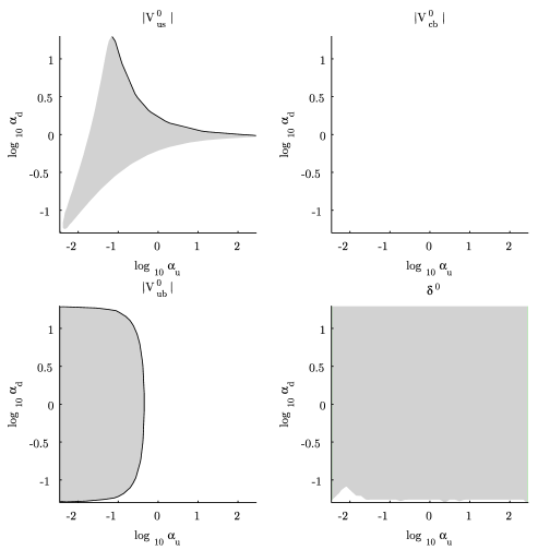
Figure 5: The allowed region in the $\alpha_{u}$ - $\alpha_{d}$ parameter plane for the case (iii) in which Type A assignment both for up quarks and down quarks are taken.

which are inconsistent with Eq. (49). In Fig. 5, allowed regions in the $\alpha_{u}-\alpha_{d}$ parameter space are derived, which are obtained from the restrictions of $|V^{0}_{us}|$, $|V^{0}_{cb}|$, $|V^{0}_{ub}|$, and the $CP$ violating phase $\delta^{0}$ in Eqs. (49) - (53), respectively with use of free $\eta_{u}$ and $\eta_{d}$ (i.e. $0\leq\eta_{u}\leq 2\pi$ and $0\leq\eta_{d}\leq 2\pi$). As seen from Fig. 5, the case (iii) is inconsistent with Eq. (53) if we use the center values of the quark masses.

We have presented the results for only the case (i), case (ii), and case (iii). For other possible cases we have no consistent allowed regions of the parameters.

V conclusion

We have proposed a mass matrix model that gives a universal description of quark and lepton with the same texture form (6), based on a flavor $2\leftrightarrow 3$ symmetry including a phase $\phi$. Against the conventional picture that the mass matrix forms in the quark sector will take somewhat different structures from those in the lepton sector, we have considered a scenario in which the flavor $2\leftrightarrow 3$ symmetry play a role in the quark mass matrices as well as in the lepton mass matrices as a fundamental common symmetry in the Yukawa couplings. By using the quark masses as inputs, the present model has four adjustable parameters, $\alpha_{u}$, $\alpha_{d}$, $\eta_{u}$, and $\eta_{d}$ to reproduce the observed CKM quark mixing matrix parameters at the electroweak scale. We have shown that the observed small CKM quark mixings are realized by a fine tuning of the parameters in the case (i) where type A assignment for up quarks and type B for down quarks are taken. With this consistent parameters, our result suggests an interesting mass matrix structure for up and down quarks, which will give a clue to a possible form of mass matrix. Since the components of each mass matrix $M_{f}$ takes different values, the present model cannot be embedded into a GUT scenario. However, it is worth-while noting that it can give a universal description of quark and lepton mass matrices with the same texture form based on a flavor $2\leftrightarrow 3$ symmetry.

*

Appendix A

Following the discussions in Ref. Matsuda , let us give a brief review of the diagonalization of mass matrix $\widehat{M}$ given by

$$\widehat{M}=\left(\begin{array}[]{lll}\ 0&\ A_{f}&\ A_{f}\\ \ A_{f}&\ B_{f}&\ C_{f}\\ \ A_{f}&\ C_{f}&\ B_{f}\\ \end{array}\right).$$ (142)

The eigenvalues of $\widehat{M}$ are given by

$$-\lambda_{1f} = \frac{1}{2}\left[B_{f}+C_{f}-\sqrt{8A_{f}^{2}+(B_{f}+C_{f})^{2}}\right],$$ (143)

$$\lambda_{2f} = \frac{1}{2}\left[B_{f}+C_{f}+\sqrt{8A_{f}^{2}+(B_{f}+C_{f})^{2}}\right],$$ (144)

$$\lambda_{3f} = B_{f}-C_{f}.$$ (145)

To the contrary, the texture’s components $A_{f}$, $B_{f}$, and $C_{f}$ are expressed in terms of $\lambda_{if}$ as

$$A_{f} = \sqrt{\frac{\lambda_{2f}\lambda_{1f}}{2}},$$

$$B_{f} = \frac{1}{2}\left(\lambda_{3f}+\lambda_{2f}-\lambda_{1f}\right),$$ (146)

$$C_{f} = -\frac{1}{2}\left(\lambda_{3f}-\lambda_{2f}+\lambda_{1f}\right).$$

Here, there are following three types of assignments for the eigenvalues $\lambda_{if}$:

(i) Type A:

In this type, the mass eigenvalues $\lambda_{1f}$, $\lambda_{2f}$, and $\lambda_{3f}$ are allocated to the masses of the first, second, and third generations, respectively. (i.e. $\lambda_{1f}$$<$$\lambda_{2f}$$<$$\lambda_{3f}$.) Therefore, $\widehat{M}$ is diagonalized by an orthogonal matrix $O_{f}$ as

$$O_{f}^{T}\widehat{M}O_{f}=\mbox{diag}(-\lambda_{1f},\lambda_{2f},\lambda_{3f}),$$ (147)

with

$$O_{f}\equiv\left(\begin{array}[]{ccc}{c_{f}}&{s_{f}}&{0}\\ {-\frac{s_{f}}{\sqrt{2}}}&{\frac{c_{f}}{\sqrt{2}}}&{-\frac{1}{\sqrt{2}}}\\ {-\frac{s_{f}}{\sqrt{2}}}&{\frac{c_{f}}{\sqrt{2}}}&{\frac{1}{\sqrt{2}}}\end{array}\right),$$ (148)

where

$$c_{f}=\sqrt{\frac{\lambda_{2f}}{\lambda_{2f}+\lambda_{1f}}},\quad s_{f}=\sqrt{\frac{\lambda_{1f}}{\lambda_{2f}+\lambda_{1f}}}.$$ (149)

(ii) Type B:

In this type, the mass eigenvalues $\lambda_{1f}$, $\lambda_{3f}$, and $\lambda_{2f}$ are allocated to the masses of the first, second, and third generations, respectively. (i.e. $\lambda_{1f}$$<$$\lambda_{3f}$$<$$\lambda_{2f}$.) Therefore, $\widehat{M}$ is diagonalized by an orthogonal matrix $O_{f}^{\prime}$ as

$$O_{f}^{\prime T}\widehat{M}O_{f}^{\prime}=\mbox{diag}(-\lambda_{1f},\lambda_{3f},\lambda_{2f}),$$ (150)

with

$$O_{f}^{\prime}\equiv\left(\begin{array}[]{ccc}{c_{f}}&{0}&{s_{f}}\\ {-\frac{s_{f}}{\sqrt{2}}}&{\frac{1}{\sqrt{2}}}&{\frac{c_{f}}{\sqrt{2}}}\\ {-\frac{s_{f}}{\sqrt{2}}}&{-\frac{1}{\sqrt{2}}}&{\frac{c_{f}}{\sqrt{2}}}\end{array}\right).$$ (151)

Here $O_{f}^{\prime}$ is obtained from $O_{f}$ by exchanging the second row for the third one.

(iii) Type C:

In this type, the mass eigenvalues $\lambda_{3f}$, $\lambda_{1f}$, and $\lambda_{2f}$ are allocated to the masses of the first, second, and third generations, respectively. (i.e. $\lambda_{3f}$$<$$\lambda_{1f}$$<$$\lambda_{2f}$.) Therefore, $\widehat{M}$ is diagonalized by an orthogonal matrix $O_{f}^{\prime\prime}$ as

$$O_{f}^{\prime\prime T}\widehat{M}O_{f}^{\prime\prime}=\mbox{diag}(\lambda_{3f},-\lambda_{1f},\lambda_{2f}),$$ (152)

with

$$O_{f}^{\prime\prime}\equiv\left(\begin{array}[]{ccc}{0}&{c_{f}}&{s_{f}}\\ {\frac{1}{\sqrt{2}}}&{-\frac{s_{f}}{\sqrt{2}}}&{\frac{c_{f}}{\sqrt{2}}}\\ {-\frac{1}{\sqrt{2}}}&{-\frac{s_{f}}{\sqrt{2}}}&{\frac{c_{f}}{\sqrt{2}}}\end{array}\right).$$ (153)

Here $O_{f}^{\prime\prime}$ is obtained from $O_{f}^{\prime}$ by exchanging the first row for the second one.

Figure 1: The relations among the components in the mass matrix, and the definition of a free $CP$ violating phase parameter $\eta_{f}$ which is independent of the mass eigenvalues.

Figure 2: The allowed region in the parameter planes for the case (i) in which Type A assignment for up quarks and type B for down quarks are taken. The dots indicate the allowed regions, in which the CKM quark mixing angles $\sin\theta_{12}^{0}$, $\sin\theta_{23}^{0}$, $\sin\theta_{13}^{0}$, and the $CP$ violating phase $\delta^{0}$ at the GUT scale satisfy the restrictions of Eq. (49), simultaneously.

Figure 3: The allowed region in the $\alpha_{u}$ - $\alpha_{d}$ parameter plane for the case (i) in which Type A assignment for up quarks and type B for down quarks are taken. The allowed regions are indicated by the dark shaded regions which are obtained from the values of the CKM quark mixing matrix elements $|V^{0}_{us}|$, $|V^{0}_{cb}|$, $|V^{0}_{ub}|$, and the $CP$ violating phase $\delta^{0}$ in Eqs. (49) - (53), respectively. The boundary with (without) black lines shows the upper (lower) limit. Here we take $\eta_{u}$ and $\eta_{d}$ as free parameters (i.e. $0\leq\eta_{u}\leq 2\pi$ and $0\leq\eta_{d}\leq 2\pi$).

Figure 4: The allowed region in the $\alpha_{u}$ - $\alpha_{d}$ parameter plane for the case (ii) in which Type B assignment for up quarks and type A for down quarks are taken.