Abstract

Using the latest determinations of several theoretical and experimental parameters, we update the Unitarity Triangle analysis in the Standard Model. The basic experimental constraints come from the measurements of $\left|V_{ub}/V_{cb}\right|$, $\Delta m_{d}$, the lower limit on $\Delta m_{s}$, $\varepsilon_{K}$, and the measurement of the phase of the $B_{d}$–$\overline{B}_{d}$ mixing amplitude through the time-dependent CP asymmetry in $B^{0}\to J/\psi K^{0}$ decays. In addition, we consider the direct determination of $\alpha$, $\gamma$, $2\beta$+$\gamma$ and $\cos 2\beta$ from the measurements of new CP-violating quantities, recently performed at the $B$ factories. We also discuss the opportunities offered by improving the precision of the various physical quantities entering in the determination of the Unitarity Triangle parameters. The results and the plots presented in this paper can also be found at the URL http://www.utfit.org, where they are continuously updated with the newest experimental and theoretical results.

1 Introduction

The Standard Model (SM) of electroweak and strong interactions provides an excellent description of all observed phenomena in particle physics up to the energies presently explored.

The LEP/SLD era of precision electroweak physics has ended, leaving us a beautiful legacy of measurements that strongly constrain alternative mechanisms of electroweak symmetry breaking [1], pointing strongly to a light Higgs boson. On the other hand, $B$ factories have thoroughly developed the study of precision $B$ physics, which, after the great achievement of the $A_{CP}(B^{0}\to J/\psi K^{0})$ measurement, is entering its mature age with many analyses aimed at measuring the angles of the Unitarity Triangle (UT) in different processes.

This remarkable experimental progress has been paralleled by many theoretical novelties: on the one hand, the consolidation of the Heavy Quark Expansion and Lattice QCD (LQCD) results on heavy mesons; on the other, the constant refinement of ideas and techniques to extract information on the UT angles from $B$ decay rates and CP asymmetries.

Waiting for LHC to uncover the mysteries connected to electroweak symmetry breaking and the hierarchy problem, we have the chance to indirectly probe scales up to a few TeV through a precision study of flavour physics. The aim of the UTfit Collaboration is twofold: i) the “classic” issue of assessing our present knowledge of flavour physics in the SM, combining all available experimental and theoretical information; ii) the future-oriented task of constraining new physics models and their parameters on the ground of flavour and CP-violating phenomena.

Up to now, the standard UT analysis [2, 3, 4] relies on the following measurements: $\left|V_{ub}\right|/\left|V_{cb}\right|$, $\Delta{m_{d}}$, the limit on $\Delta{m_{s}}$, and the measurements of CP-violating quantities in the kaon ($\varepsilon_{K}$) and in the $B$ ($\sin{2\beta}$) sectors. Inputs to this analysis consist of a large body of both experimental measurements and theoretically determined parameters, where LQCD calculations play a central rôle. A careful choice (and a continuous update) of the values of these parameters is a prerequisite in this study. The values and errors attributed to these parameters in the present study are summarized in Table 1 (Section 2). The results of the analysis and the determination of the UT parameters are presented and discussed in Section 3 which is an update of similar analyses performed in [2, 3] to which the reader can refer for more details.

New CP-violating quantities have been recently measured by the $B$ factories, allowing for the determination of several combinations of UT angles. The measurements of $\alpha$ (using $\pi\pi$, $\rho\rho$ and $\pi\rho$ modes), $\gamma$ (using $D^{(*)}K^{(*)}$ modes), $2\beta+\gamma$ (using $D^{(*)}\pi(\rho)$ modes), and $\cos 2\beta$ from $B^{0}\to J/\psi K^{*}$ are now available. These measurements and their effect on the UT fit are discussed in Section 4.

Finally in Section 5 we discuss the perspectives opened by improving the precision in the measurements of various physical quantities entering the UT analysis. In particular, we investigate to which extent future and improved determinations of the experimental constraints, such as $\sin 2\beta$, $\Delta m_{s}$, $\alpha$ and $\gamma$, could allow us to invalidate the SM, thus signalling the presence of new physics effects.

2 Inputs used for the “standard” analysis

The values and errors of the relevant quantities used in this paper for the standard analysis of the CKM parameters (corresponding to the constraints from $\left|V_{ub}\right|/\left|V_{cb}\right|$, $\Delta{m_{d}}$, $\Delta{m_{s}}/\Delta{m_{d}}$, $\varepsilon_{K}$ and $\sin{2\beta}$) are summarized in Table 1.

The novelties here are the final LEP/SLD likelihood for $\Delta m_{s}$, the use of $|V_{ub}|$ measurements from inclusive semileptonic decays at the $B$ factories [5], the updated value of $\sin{2\beta}$ and a new treatment of the non-perturbative QCD parameters as explained in the following Section 2.1. In addition, we use updated values of the top mass $m_{t}^{\rm pole}=178.0\pm 4.3$ GeV [6] and of the CKM parameter $\lambda$. The latter comes from the average of the following values [7]

$$\lambda(V_{us}~{}{\rm from}~{}K_{l3}) = 0.2250\pm 0.0021$$

$$\lambda(V_{ud}+~{}{\rm unitarity}) = 0.2265\pm 0.0020.$$ (1)

Finally, we now calculate QCD corrections to $\Delta B=2$ and $\Delta S=2$ processes, fully taking into account their correlations with the input parameters and, by varying the matching scale, the uncertainty introduced by the residual scale dependence.

Parameter	Value	Gaussian ($\sigma$)	Uniform
			(half-width)
$\lambda$	0.2258	0.0014	-
$\left|V_{cb}\right|$(excl.)	$41.4\times 10^{-3}$	$2.1\times 10^{-3}$	-
$\left|V_{cb}\right|$(incl.)	$41.6\times 10^{-3}$	$0.7\times 10^{-3}$	$0.6\times 10^{-3}$
$\left|V_{ub}\right|$(excl.)	$33.0\times 10^{-4}$	$2.4\times 10^{-4}$	$4.6\times 10^{-4}$
$\left|V_{ub}\right|$(incl.)	$47.0\times 10^{-4}$	$4.4\times 10^{-4}$	-
$\Delta m_{d}$	$0.502~{}\mbox{ps}^{-1}$	$0.006~{}\mbox{ps}^{-1}$	-
$\Delta m_{s}$	$>$ 14.5 ps-1 at 95% C.L.	sensitivity 18.3 ps-1
$f_{B_{s}}\sqrt{\hat{B}_{B_{s}}}$	$276$ MeV	$38$ MeV	-
$\xi=\frac{f_{B_{s}}\sqrt{\hat{B}_{B_{s}}}}{f_{B_{d}}\sqrt{\hat{B}_{B_{d}}}}$	1.24	0.04	0.06
$\hat{B}_{K}$	0.86	0.06	0.14
$\varepsilon_{K}$	$2.280\times 10^{-3}$	$0.013\times 10^{-3}$	-
$f_{K}$	0.159 GeV	fixed
$\Delta m_{K}$	0.5301 $\times 10^{-2}~{}\mbox{ps}^{-1}$	fixed
$\sin{2\beta}$	0.726	0.037	-
$\overline{m}_{t}$	$168.5$ GeV	$4.1$ GeV	-
$\overline{m}_{b}$	4.21 GeV	0.08 GeV	-
$\overline{m}_{c}$	1.3 GeV	0.1 GeV	-
$\alpha_{s}(M_{Z})$	0.119	0.003	-
$G_{F}$	1.16639 $\times 10^{-5}\rm{GeV}^{-2}$	fixed
$m_{W}$	80.425 GeV	fixed
$m_{B^{0}_{d}}$	5.279 GeV	fixed
$m_{B^{0}_{s}}$	5.375 GeV	fixed
$m_{K}^{0}$	0.497648 GeV	fixed

Table 1: Values of the relevant quantities used in the UT fit. The Gaussian and the flat contributions to the uncertainty are given in the third and fourth columns respectively (for details on the statistical treatment see [2]).

2.1 Use of $\xi$, $f_{B_{s}}\sqrt{\hat{B}_{B_{s}}}$ and $f_{B_{d}}\sqrt{\hat{B}_{B_{d}}}$ in $\Delta m_{s}$ and $\Delta m_{d}$ constraints

One of the important differences with respect to previous studies is in the use of the information from non-perturbative QCD parameters entering the expressions of $\Delta m_{s}$ and $\Delta m_{d}$. The $B_{s}$–${\overline{B}}_{s}$ mass difference is proportional to the square of the element $|V_{ts}|$. Up to Cabibbo-suppressed corrections, $|V_{ts}|$ is independent of $\overline{\rho}$ and $\overline{\eta}$. As a consequence, the measurement of $\Delta m_{s}$ would provide a strong constraint on the non-perturbative QCD parameter $f_{B_{s}}^{2}\hat{B}_{B_{s}}$.

We propose a new and more appropriate way of treating the constraints coming from the measurements of $\Delta m_{s}$ and $\Delta m_{d}$. In previous analyses, these constraints were implemented using the following equations

$$\Delta m_{d} \propto [(1-\overline{\rho})^{2}+\overline{\eta}^{2}]f_{B_{d}}^{2}\hat{B}_{B_{d}}$$ (2)

$$\Delta m_{s} \propto f_{B_{s}}^{2}\hat{B}_{B_{s}}=f_{B_{d}}^{2}\hat{B}_{B_{d}}\times\xi^{2}$$

where $\xi=f_{B_{s}}\sqrt{\hat{B}_{B_{s}}}/f_{B_{d}}\sqrt{\hat{B}_{B_{d}}}$. In this case, the input quantities are $f_{B_{d}}\sqrt{\hat{B}_{B_{d}}}$ and $\xi$. The constraints from $\Delta m_{s}$ and the knowledge of $\xi$ are used to improve the knowledge on $f_{B_{d}}\sqrt{\hat{B}_{B_{d}}}$ which thus makes the constraint on $\Delta m_{d}$ more effective.

The hadronic parameter that is better determined from lattice calculations, however, is $f_{B_{s}}^{2}\hat{B}_{B_{s}}$, whereas $\xi$ and $f_{B_{d}}^{2}\hat{B}_{B_{d}}$ are affected by larger uncertainties coming from the chiral extrapolations. These uncertainties are strongly correlated. For this reason, a better approach consists in replacing Eq. (2) with

$$\Delta m_{d} \propto [(1-\overline{\rho})^{2}+\overline{\eta}^{2}]\frac{f_{B_{s}}^{2}\hat{B}_{B_{s}}}{\xi^{2}}$$ (3)

$$\Delta m_{s} \propto f_{B_{s}}^{2}\hat{B}_{B_{s}}.$$

At present, this new parameterization does not have a large effect on the final results. It allows, however, to take into account more accurately the uncertainty from the chiral extrapolation in lattice calculations of $f_{B_{d}}$. Note that in this way, in order to obtain a more effective constraint on $\Delta m_{d}$, the error on $\xi$ should also be improved.

3 Determination of the Unitarity Triangle parameters: the standard analysis

Figure 1: From top to bottom and from left to right, the a-posteriori p.d.f.’s for $\overline{\rho}$, $\overline{\eta}$, $\alpha$, $\sin{2\beta}$, $\gamma$ and $\sin(2\beta+\gamma)$. The red (darker) and the yellow (lighter) zones correspond respectively to 68% and 95% of the area. The following constraints have been used in the UT fit: $\left|V_{ub}/|V_{cb}\right|$, $\Delta m_{d}$, $\Delta m_{s}$, $\varepsilon_{K}$, and $\sin{2\beta}$ from the measurement of the CP asymmetry in the $J/\psi K^{0}$ decays.

Figure 2: Allowed regions for $\overline{\rho}$ and $\overline{\eta}$ using the parameters listed in Table 1. The closed contours at 68% and 95% probability are shown. The full lines correspond to 95% probability regions for each of the constraints, given respectively by the measurements of $\left|V_{ub}\right|/\left|V_{cb}\right|$, $\Delta m_{d}$, $\Delta m_{s}$, $\varepsilon_{K}$, and $\sin{2\beta}$ from the measurement of the CP asymmetry in the $J/\psi K^{0}$ decays.

Using the constraints from $\left|V_{ub}\right|/\left|V_{cb}\right|$, $\Delta{m_{d}}$, $\Delta{m_{s}}$, $\varepsilon_{K}$ and $\sin{2\beta}$, we obtain the results given in Table 2. The central value for each p.d.f. is calculated using the median and the error corresponds to $34\%$ probability regions on each side of the median. Asymmetric errors are symmetrized changing the quoted central value.  Figures 1 and 2 show, respectively, the probability density functions (p.d.f.’s) for some UT parameters and the selected region in the $\overline{\rho}-\overline{\eta}$ plane.

Parameter	68$\%$	95$\%$	99$\%$
$\overline{\rho}$	0.196 $\pm$ 0.045	[0.104, 0.283]	[0.073, 0.314]
$\overline{\eta}$	0.347 $\pm$ 0.025	[0.296, 0.396]	[0.281, 0.412]
$\alpha[^{\circ}]$	96.1 $\pm$ 7.0	[82.1, 110.0]	[77.7, 114.8]
$\beta[^{\circ}]$	23.4 $\pm$ 1.5	[20.8, 26.1]	[20.2, 27.1]
$\gamma[^{\circ}$]	60.3 $\pm$ 6.8	[47.0, 74.2]	[42.5, 78.9]
$\sin 2\alpha$	-0.21 $\pm$ 0.24	[-0.65, 0.27]	[-0.77, 0.41]
$\sin{2\beta}$	0.726 $\pm$ 0.028	[0.670, 0.780]	[0.651, 0.797]
$\sin(2\beta+\gamma)$	0.947 $\pm$ 0.038	[0.852, 0.996]	[0.813, 0.998]
$\rm{Im}{\lambda}_{t}$[$10^{-5}$]	13.3 $\pm$ 0.9	[11.5, 15.1]	[10.9, 15.6]

Table 2: Values and probability ranges for the UT parameters obtained from the UT fit using the following constraints: $\left|V_{ub}\right|/\left|V_{cb}\right|$, $\Delta{m_{d}}$, $\Delta{m_{s}}$, $\varepsilon_{K}$ and $\sin{2\beta}$. The value of $\rm{Im}{\lambda}_{t}=\rm{Im}{V^{*}_{ts}V_{td}}$ is also given.

3.1 Fundamental test of the Standard Model in the quark sector

Figure 3: The allowed regions for $\overline{\rho}$ and $\overline{\eta}$ (close contours at 68%, 95% probability ranges), as selected by the measurements of $\left|V_{ub}\right|/\left|V_{cb}\right|$, $\Delta{m_{d}}$, and by the limit on $\Delta{m_{s}}$, are compared with the bands (at 68% and 95% probability ranges) from the measurements of CP-violating quantities in the kaon ($\varepsilon_{K}$) and in the B ($\sin{2\beta}$) sectors.

The standard fit, illustrated in Figure 2, gives a clear picture of the success of the SM. A crucial test consists in establishing CP violation by using the sides of the UT, i.e. CP-conserving processes such as the semileptonic $B$ decays and $B_{d,s}-{\overline{B}}_{d,s}$ oscillations. The comparison of the region selected by these constraints and the one selected by the direct measurements of CP violation in the kaon ($\varepsilon_{K}$) or in the $B$ ($\sin{2\beta}$) sectors is shown in Figure 3 and gives a picture of the success of the SM in the flavour sector. This pictorial agreement is quantified through the comparison between the value of $\overline{\rho}$ and $\overline{\eta}$ computed from CP-conserving and CP-violating observables: 

$$\left.\begin{array}[]{l}\overline{\rho}=0.169\pm 0.057([0.055,\,0.310]~{}{\rm at}~{}95\%)\\ \overline{\eta}=0.364\pm 0.037([0.252,\,0.430]~{}{\rm at}~{}95\%)\end{array}\right\}~{}~{}\rm{UT~{}sides~{}only}$$ (6)

$$\left.\begin{array}[]{l}\overline{\rho}=0.241\pm 0.070([0.098,\,0.363]~{}{\rm at}~{}95\%)\\ \overline{\eta}=0.311\pm 0.030([0.260,\,0.371]~{}{\rm at}~{}95\%)\end{array}\right\}~{}~{}\rm{S(J/\psi K^{0})+\varepsilon_{K}}$$ (9)

Another test can be performed by comparing the value of $\sin{2\beta}$ from $S(J/\psi K^{0})$ and the one determined from “sides” measurements

$$\sin{2\beta}= 0.734\pm 0.043~{}([0.616,0.811]~{}{\rm at}~{}95\%) ~{}~{}\rm{UT~{}sides~{}only}$$

$$\sin{2\beta}= 0.726\pm 0.037~{}([0.652,0.800]~{}{\rm at}~{}95\%) ~{}~{}S(J/\psi K^{0})$$ (10)

For completeness, we also give the value of $\sin{2\beta}$ obtained by using all the constraints but the direct determination:

$$\sin{2\beta}=0.725\pm 0.043~{}([0.634,0.804]~{}{\rm at}~{}95\%)~{}~{}\rm{UT~{}sides}+\epsilon_{K}.$$ (11)

As a matter of fact, the value of $\sin{2\beta}$ was predicted, before its first direct measurement was obtained, by using all other available constraints ($\left|V_{ub}\right|/\left|V_{cb}\right|$, $\Delta m_{d}$, $\Delta m_{s}$, and $\varepsilon_{K}$). The “indirect” determination has improved regularly over the years, as shown in Figure 4, where the direct measurement is also reported, as a reference.

The agreement of these determinations confirms the validity of CKM mechanism in the SM. This test relies on several non-perturbative techniques, such as the Operator Product Expansion for computing $B$ decay rates, the Heavy Quark Effective Theory and LQCD, which are used to extract the CKM parameters from the experimental measurements. The overall consistency of the UT fit gives confidence on the theoretical tools. Assuming the validity of the SM, it is possible to perform a more quantitative test of the non-perturbative techniques as discussed in following.

Figure 4: Evolution of the “indirect” determination of $\sin{2\beta}$ over the years (until 2002). From left to right, they correspond to the following papers [4, 8]: dRLMPPPPS90, DDGN90, LMMR92, AL94, CFMRS95, BBL95, AL96, PPRS97, BF97, BPS98, PS98, AL99, CFGLM99, CPRS99, M99, CDFLMPRS00, B.et.al.00, HLLL00 and CFLPSS [2, 3]. The dotted lines correspond to the 95$\%$ C.L. regions (the only information given in those papers). The larger hatched bands (from year ’99) correspond to values of $\sin{2\beta}$ from direct measurements ($\pm 1\sigma$). The most recent values contained in this paper are also shown.

3.2 Determination of other quantities

In the previous sections we have obtained the a-posteriori p.d.f.’s for all the UT parameters. It is also instructive to remove from the fitting procedure the external information on the value of one (or more) of the constraints.

In this section we study the distributions of $\Delta m_{s}$ and of the hadronic parameters. In the first case we do not include in the analysis the experimental information on $B_{s}$–${\overline{B}}_{s}$ mixing coming from LEP and SLD. In the case of the hadronic parameters, we remove from the fit the constraints on their values coming from lattice calculations, and use them as free parameters of the fit. In this way we can compare the uncertainty obtained on a given quantity through the UT fit to the present theoretical error on the same quantity.

3.2.1 The expected distribution for $\Delta m_{s}$

The p.d.f. for $\Delta m_{s}$ obtained by removing the experimental information coming from $B_{s}$–${\overline{B}}_{s}$ mixing is shown in Figure 5. The result of this exercise is given in Table 3 (upper line). The present experimental analyses of $B_{s}$–${\overline{B}}_{s}$ mixing at LEP and SLD have established a sensitivity of 18.3 ps^-1 and they show an evidence at about 2$\sigma$ for a positive signal at around 17.5 ps^-1, well compatible with the range of the $\Delta m_{s}$ distribution from the UT fit (Figure 5). The inclusion of this information in the UT analysis has a large impact on the determination of $\Delta m_{s}$, as shown by the comparison between the permitted range obtained when this information is either included or not (see Table 3). Accurate measurements of $\Delta m_{s}$, expected from the TeVatron in the near future, will provide an ingredient of the utmost importance for testing the SM.

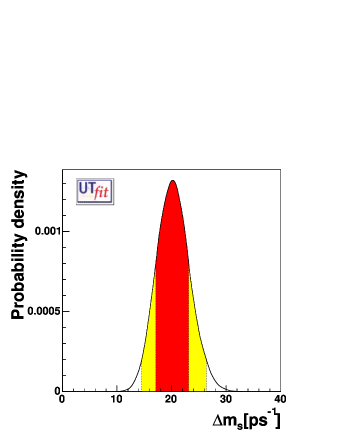
Figure 5: $\Delta m_{s}$ probability distribution, obtained without using the experimental information from $B_{s}$–${\overline{B}}_{s}$ mixing.

Parameter	68$\%$	95$\%$	99$\%$
$\Delta m_{s}$(without $\Delta m_{s}$) [ps-1]	21.2 $\pm$ 3.2	[15.4, 27.8]	[13.8, 30.0]
$\Delta m_{s}$(including  $\Delta m_{s}$) [ps-1]	18.5 $\pm$ 1.6	[15.6, 23.1]	[15.1, 27.3]

Table 3: Central values and ranges for $\Delta m_{s}$ corresponding to defined levels of probability, obtained by including (or not) the experimental information on $\Delta m_{s}$.

3.2.2 Determination of $f_{B_{s}}\sqrt{\hat{B}_{B_{s}}}$, $\hat{B}_{K}$ and $\xi$

To obtain the a-posteriori p.d.f. for a given hadronic quantity, we perform the UT fit imposing as input a uniform distribution in a range much larger than the expected interval of values assumed for the quantity itself. Table 4 and Figure 6 (left column) show the results when one single parameter is taken out of the fit with the above procedure. The central value and the error of each of these quantities have to be compared to the current evaluations from LQCD, given in Table 1 and also shown in Table 4 for the reader’s convenience.

Parameter	68$\%$	95$\%$	99$\%$
$\xi$ -UTfit	1.15 $\pm$ 0.11	[0.97, 1.44]	[0.93, 1.59]
$\xi$ -LQCD	1.24 $\pm$ 0.06	[1.13, 1.34]	[1.10, 1.37]
$f_{B_{s}}\sqrt{\hat{B}_{B_{s}}}$(MeV) -UTfit	265 $\pm$ 13	[242, 305]	[236, 330]
$f_{B_{s}}\sqrt{\hat{B}_{B_{s}}}$(MeV) -LQCD	276 $\pm$ 38	[201, 350]	[179, 373]
$\hat{B}_{K}$ -UTfit	0.69 $\pm$ 0.10	[0.53, 0.93]	[0.49, 1.07]
$\hat{B}_{K}$ -LQCD	0.86 $\pm$ 0.11	[0.67, 1.05]	[0.62, 1.10]

Table 4: Values and probability ranges for the non-perturbative QCD parameters, if the external information (input) coming from the theoretical calculation of these parameters is not used in the fit. The LQCD values are given with errors obtained by convoluting the Gaussian and flat contributions reported separately in Table 1.

Some conclusions can be drawn. The precision on $f_{B_{s}}\sqrt{\hat{B}_{B_{s}}}$ obtained from the fit has an accuracy which is better than the current evaluation from LQCD. This proves that the standard UT fit is, in practice, weakly dependent on the assumed theoretical uncertainty on $f_{B_{s}}\sqrt{\hat{B}_{B_{s}}}$.

The result on $\hat{B}_{K}$ indicates that values of $\hat{B}_{K}$ smaller than $0.49$ are excluded at $99\%$ probability, while large values of $\hat{B}_{K}$ are compatible with the prediction of the fit obtained using the other constraints. The present estimate of $\hat{B}_{K}$ from LQCD, which has a 15$\%$ relative error (Table 1), is as precise as the indirect determination from the UT fit.

The present best determination of the parameter $\xi$ comes from LQCD.

In the above exercise we have removed from the fit individual quantities one by one. It is also interesting to see what can be obtained taking out two of them simultaneously. Figure 6 shows the regions selected in the planes ($f_{B_{s}}\sqrt{\hat{B}_{B_{s}}}$, $\hat{B}_{K}$), ($\hat{B}_{K}$, $\xi$) and ($f_{B_{s}}\sqrt{\hat{B}_{B_{s}}}$, $\xi$). The corresponding results are summarized in Table 5. For ($f_{B_{s}}\sqrt{\hat{B}_{B_{s}}}$, $\xi$), the 2-dimensional distribution is not limited by the fit. In such a case, the probability attached to a given range depends completely on the ranges of the a-priori distributions chosen for the two variables. For this reason, we do not quote any range in Table 5. Still, from the plot in Figure 6, a combined lower bound $f_{B_{s}}\sqrt{\hat{B}_{B_{s}}}\gtrsim 200$ MeV and $\xi\gtrsim 0.9$ emerges.

Parameter	68$\%$	95$\%$	99$\%$
$\hat{B}_{K}$	0.68$\pm$ 0.10	[0.52, 0.97]	[0.48, 1.21]
$f_{B_{s}}\sqrt{\hat{B}_{B_{s}}}$(MeV)	257 $\pm$ 15	[232, 304]	[221, 348]
$\hat{B}_{K}$	0.68 $\pm$ 0.18	[0.45,1.14]	[0.41,1.33]
$\xi$	1.31 $\pm$ 0.21	[0.96,1.72]	[0.89,1.98]

Table 5: Values and probability ranges for the non-perturbative QCD parameters, if two external pieces of information (inputs) coming from the theoretical calculations of these parameters are not used in the fit.

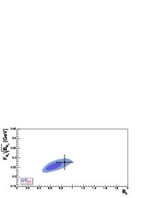
Figure 6: One- and two-dimensional probability distributions for $\hat{B}_{K}$, $\xi$ and $f_{B_{s}}\sqrt{\hat{B}_{B_{s}}}$ (see Section 3.2.2). The dark and the light (blue) zones correspond respectively to 68% and 95% of the area. The 1$\sigma$ ranges for these quantities, as calculated from LQCD, are indicated with error bars.

4 New Constraints from UT angle measurements

The values for $\alpha$, $\gamma$, $\sin(2\beta+\gamma)$, and $\sin 2\beta$ given in Table 2 have to be taken as predictions for future measurements. A strong message is given for instance for the angle $\gamma$. Its indirect determination is known with an accuracy of about $10\%$.

Thanks to the huge statistics collected at the $B$ factories, new CP-violating quantities have been recently measured allowing for the direct determination of $\alpha$, $\gamma$, $2\beta$+$\gamma$, and $\cos 2\beta$. In the following, we study the constraints induced by these new measurements in the $\overline{\rho}-\overline{\eta}$ plane and their impact on the global UT fit.

4.1 Determination of the angle $\gamma$ using $DK$ events

Various methods related to $B\to DK$ decays have been proposed to determine the UT angle $\gamma$ [9]-[11], using the fact that a charged $B$ can decay into a $D^{0}(\overline{D}^{0})K$ final state via a $V_{cb}$($V_{ub})$ mediated process. CP violation occurs if the $D^{0}$ and the $\overline{D}^{0}$ decay to the same final state. These processes are thus sensitive to the phase difference $\gamma$ between $V_{ub}$ and $V_{cb}$. The same argument can be applied to $B\to D^{*}K$ and $B\to D^{(*)}K^{*}$ decays.

Three methods have been proposed:

• Gronau-London-Wyler method (GLW) [9]. It consists in reconstructing the neutral $D$ meson in a CP eigenstate: $B^{\pm}\to D^{0}_{CP^{\pm}}K^{\pm}$, where $D^{0}_{CP^{\pm}}$ are the CP eigenstates of the $D$ meson. In this case, one can define four quantities, sensitive to the value of the angle $\gamma$:

  $$R_{C\!P^{\pm}}=\frac{\Gamma(B^{+}\to D^{0}_{CP^{\pm}}K^{+})+\Gamma(B^{-}\to D^{0}_{CP^{\pm}}K^{-})}{\Gamma(B^{+}\to D^{0}K^{+})+\Gamma(B^{-}\to\overline{D}^{0}K^{-})}=1+r_{B}^{2}\pm 2r_{B}\cos\gamma\cos\delta_{B}$$

  $$A_{C\!P^{+}}=\frac{\Gamma(B^{+}\to D^{0}_{CP^{\pm}}K^{+})-\Gamma(B^{-}\to D^{0}_{CP^{\pm}}K^{-})}{\Gamma(B^{+}\to D^{0}_{CP^{\pm}}K^{+})+\Gamma(B^{-}\to D^{0}_{CP^{\pm}}K^{-})}=\frac{\pm 2r_{B}\sin\gamma\sin\delta_{B}}{R_{C\!P^{\pm}}}$$ (12)

  where $r_{B}$ is the absolute value of the ratio of the Cabibbo-suppressed over the Cabibbo-allowed amplitudes:

  $$r_{B}(DK)=\left|\frac{{\cal A}(B^{-}\to\overline{D}^{0}K^{-})}{{\cal A}(B^{-}\to{D}^{0}K^{-})}\right|.$$ (13)

  The phase $\delta_{B}$ in Eq. (12) is the strong phase difference between the $b\to u$ and the $b\to c$ decays. The main limitation of this method comes from the dilution of the interference effect, since $r_{B}$ is expected to be small ($\sim|V_{ub}/V_{cb}|$). One can nevertheless repeat this measurement for several $f_{CP}$ final states of $D$ meson. Moreover, this method (and the ones introduced below) can be generalized to $D^{*}K$, $DK^{*}$ and $D^{*}K^{*}$ final states, having different values for $r_{B}$ and $\delta_{B}$, but the same functional dependence on $\gamma$. In case of $B\to D^{*}K$ decays, there is an effective strong-interaction phase difference of $180^{\circ}$ whenever the $D^{*}$ is reconstructed as $D^{*}\to D\gamma$ or $D^{*}\to D\pi$ [12].

• Atwood-Dunietz-Soni method (ADS) [10]. It consists in forcing the $\bar{D}^{0}$ ($D^{0}$) meson, coming from the Cabibbo-suppressed (Cabibbo-allowed) $b\to u$ ($b\to c$) transition to decay into the Cabibbo-allowed (Cabibbo-suppressed) $K\pi$ final state. In this way, one can look at the interference between two amplitudes having the same order of magnitude. Two quantities are defined:

  $$R_{ADS} = \frac{\Gamma(B^{-}\to[K^{+}\pi^{-}]_{D}K^{-})+\Gamma(B^{+}\to[K^{-}\pi^{+}]_{D}K^{+})}{\Gamma(B^{-}\to[K^{-}\pi^{+}]_{D}K^{-})+\Gamma(B^{+}\to[K^{+}\pi^{-}]_{D}K^{+})}$$

  $$= r_{DCS}^{2}+r_{B}^{2}+2r_{B}r_{DCS}\cos\gamma\cos(\delta_{B}+\delta_{D})$$

  $$A_{ADS} = \frac{\Gamma(B^{-}\to[K^{+}\pi^{-}]_{D}K^{-})-\Gamma(B^{+}\to[K^{-}\pi^{+}]_{D}K^{+})}{\Gamma(B^{-}\to[K^{+}\pi^{-}]_{D}K^{-})+\Gamma(B^{+}\to[K^{-}\pi^{+}]_{D}K^{+})}$$ (14)

  $$= 2r_{B}r_{DCS}\sin\gamma\sin(\delta_{B}+\delta_{D})/R_{ADS}$$

  which are functions (as in the case of the GLW method) of $\gamma$, $r_{B}$ and $\delta_{B}$. Since in this case $D^{0}$ and $\bar{D}^{0}$ are forced to decay into different final states, the expressions in Eq. (14) also depend on the ratio of the Cabibbo-suppressed over the Cabibbo-allowed decays of the $D$,

  $$r_{DCS}=\left|\frac{{\cal A}(D^{0}\to K^{+}\pi^{-})}{{\cal A}(D^{0}\to K^{-}\pi^{+})}\right|,$$ (15)

  and on the additional strong phase shift $\delta_{D}$ introduced by these decays. One can also use $D^{*}K$, $DK^{*}$ and $D^{*}K^{*}$, having different values of $r_{B}$ and $\delta_{B}$, but the same values of $\gamma$, $r_{DCS}$ and $\delta_{D}$.

• Dalitz method [11]. It consists in studying the interference between the $b\to u$ and the $b\to c$ transitions using the Dalitz plot of $D$ mesons reconstructed into three-body final states (such as, for instance, $D^{0}\to K_{s}\pi^{-}\pi^{+}$). The advantage of this method is that the full sub-resonance structure of the three-body decay is considered, including interferences such as those used for GLW and ADS methods plus additional interferences due to the overlap between broad resonances in some regions of the Dalitz plot. The same analysis is also performed using $B\to D^{*0}K$ decays. The Dalitz analysis has only a twofold discrete ambiguity ($\gamma,\gamma-\pi$) and not a fourfold ambiguity as in the case of the GLW and ADS methods. One can fit the experimental data to extract a 3D likelihood as a function of $r_{B}$, $\gamma$ and $\delta_{B}$.

Figure 7: Left column: a-posteriori one-dimensional p.d.f.’s (from top-left to bottom-left) for $r_{B}(DK)$, $r_{B}(D^{*}K)$, $r_{B}(DK^{*})$ and $\gamma$, using the results from $B\to D^{(*)}K^{(*)}$ decays. The plots on the right show the measurement of the angle $\gamma$ in the $\gamma-r_{B}$ (first three rows) and $\overline{\rho}-\overline{\eta}$ planes (bottom).

Both BaBar and Belle have presented results applying the three methods to several final states. It is important to notice that in the case of ADS and Dalitz measurements we used directly the experimental likelihood because of the presence of non-Gaussian effects: For Dalitz analyses, there are non-trivial correlations between $r_{B}$ and $\gamma$ and the error on $\gamma$ is proportional to $1/r_{B}$; for ADS analyses, the likelihood of $R_{ADS}$ is bounded to be positive.

Observable	$DK$	$D^{*}K$	$DK^{*}$
$A_{C\!P^{+}}$(GLW)	0.22 $\pm$ 0.11	-0.14 $\pm$ 0.18	-0.07 $\pm$ 0.18
$A_{C\!P^{-}}$(GLW)	0.02 $\pm$ 0.12	0.26 $\pm$ 0.26	-0.16 $\pm$ 0.29
$R_{C\!P^{+}}$(GLW)	0.91 $\pm$ 0.12	1.25 $\pm$ 0.20	1.77 $\pm$ 0.39
$R_{C\!P^{-}}$(GLW)	1.02 $\pm$ 0.12	0.94 $\pm$ 0.29	0.76${}^{+0.30}_{-0.33}$
$R_{ADS}$	0.017 $\pm$ 0.009	$<0.16$@90$\%$ C.L.	-
$A_{ADS}$	0.49${}^{+0.53}_{-0.46}$	-	-
$r_{B}$(Dalitz)-Belle	$0.21\pm 0.08\pm 0.03\pm 0.04$	$0.12^{+0.16}_{-0.11}\pm 0.02\pm 0.04$	-
$\gamma$$[^{\circ}]$(Dalitz)-Belle	$68\pm 15\pm 13\pm 11$	$75\pm 57\pm 11\pm 11$	-
$r_{B}$(Dalitz)-BaBar	$<0.19~{}@90\%~{}{\rm C.L.}$	$0.155^{+0.070}_{-0.077}\pm 0.040\pm 0.020$	-
$\gamma$$[^{\circ}]$(Dalitz)-BaBar	$70\pm 26\pm 10\pm 10$		-

Table 6: Summary of the experimental results obtained at the B factories from $B\to D^{(*)}K^{(*)}$ decays using the GLW, ADS and Dalitz methods [5, 13]. The last two lines give the results from the Dalitz analysis, for which the ambiguity $\gamma\to\pi-\gamma$ is implicit.

The p.d.f.’s of $\gamma$ and $r_{B}$, and the selected region in the $\gamma-r_{B}$ plane are shown in Figure 7, together with the impact of this measurement on the $\overline{\rho}-\overline{\eta}$ plane.

Figure 8: Regions of the $\overline{\rho}$–$\overline{\eta}$ plane selected by the constraints imposed by the determination of $|V_{ub}/V_{cb}|$ and $\gamma$ from tree-level processes.

The comparison between the direct and the indirect determination is:

$$\gamma[^{\circ}] = ~{}~{}~{}~{}~{}~{}~{}~{}60.3\pm 6.8~{}~{}~{}~{}([47.0,\,74.2]~{}{\rm at~{}95\%})~{}~{}~{}~{}~{}~{}~{}~{}~{}~{}~{}\rm{indirect-{\mbox{{\bf{U}}\kern-2.40005pt{\bf{T}}\kern-2.10007pt{\it{fit}}\@}}}$$ (16)

$$\gamma[^{\circ}] = \left\{\begin{array}[]{l}59.1\pm 16.7~{}~{}\cup~{}~{}-120.3\pm 17.2\\ {}([24.7,\,97.9]~{}~{}\cup~{}~{}[-155.4,\,-82.7]~{}{\rm at~{}95\%})\end{array}\right.~{}~{}\,\rm{direct-{\it D^{(*)}K^{(*)}}}$$ (19)

where the two values of the direct determination approximately correspond to the discrete ambiguity of the Dalitz method, which dominates the determination of $\gamma$. An important result of this analysis is also the distributions for the different $r_{B}$’s:

$$r_{B}(DK) = 0.10\pm 0.04~{}([0.03,\,0.17]~{}{\rm at}~{}95\%~{}C.L.)$$ (20)

$$r_{B}(D^{*}K) = 0.09\pm 0.04~{}([0.01,\,0.18]~{}{\rm at}~{}95\%~{}C.L.)$$

$$r_{B}(DK^{*}) = 0.32\pm 0.21~{}([0.02,\,0.74]~{}{\rm at}~{}95\%~{}C.L.)$$

The small values for $r_{B}(DK)$ and $r_{B}(D^{*}K)$ are limiting the precision on the present determination of $\gamma$.

It is interesting to observe that the determination of $\gamma$ discussed in this section is not affected by new physics (NP) under the mild assumption that NP does not change tree-level processes. Therefore, together with the measurement of $|V_{ub}/V_{cb}|$, it already provides a constraint on the $\overline{\rho}$–$\overline{\eta}$ plane which must be fulfilled by any NP model. The regions selected by these two constraints are shown in Figure 8. We obtain

$$\bar{\rho}=\pm(0.21\pm 0.10),~{}~{}~{}\bar{\eta}=\pm(0.36\pm 0.06).$$ (21)

A more detailed and quantitative analysis of the impact of the UT fit on specific NP models will be presented in a forthcoming paper.

4.2 Determination of $2\beta$+$\gamma$ using $D^{(*)}\pi(\rho)$ events

The interference effects between the $b\to c$ and $b\to u$ decay amplitudes in the time-dependent asymmetries of $B$ decaying into $D^{(*)}\pi$ and $D^{(*)}\rho$ final states allow for the determination of $2\beta$+$\gamma$. The time-dependent rates, in the case of $D\pi$ final states, can be written as

$$R(B^{0}\to D^{-}\pi^{+})=N~{}e^{-\Gamma t}~{}{(1+C~{}\cos(\Delta m_{d}t)+S~{}\sin(\Delta m_{d}t)~{})}$$ (22)

$$R(\overline{B}^{0}\to D^{-}\pi^{+})=N~{}e^{-\Gamma t}~{}{(1-C~{}\cos(\Delta m_{d}t)-S~{}\sin(\Delta m_{d}t)~{})}$$

$$R(B^{0}\to D^{+}\pi^{-})=N~{}e^{-\Gamma t}~{}{(1+C~{}\cos(\Delta m_{d}t)-\overline{S}~{}\sin(\Delta m_{d}t)~{})}$$

$$R(\overline{B}^{0}\to D^{+}\pi^{-})=N~{}e^{-\Gamma t}~{}{(1-C~{}\cos(\Delta m_{d}t)+\overline{S}~{}\sin(\Delta m_{d}t)~{})}$$

where $S$, $\overline{S}$ and $C$ are defined as

$$S\equiv S(D^{-}\pi^{+}) = 2\frac{r}{1+r^{2}}\sin(2\beta+\gamma-\delta)$$ (23)

$$\overline{S}\equiv S(D^{+}\pi^{-}) = 2\frac{r}{1+r^{2}}\sin(2\beta+\gamma+\delta)$$

$$C = \frac{1-r^{2}}{1+r^{2}}$$

and $r$ and $\delta$ are the absolute value and the strong phase of the amplitude ratio ${\cal A}(\overline{B}^{0}\to D^{-}\pi^{+})/{\cal A}(B^{0}\to D^{-}\pi^{+})$. All these expressions can be generalized to the case of $D^{*}\pi$ and $D\rho$ final states, which have in principle different values of $r$ and $\delta$. The ratio $r$ is expected to be rather small being of the order of $\lambda|V_{ub}/V_{cb}|\simeq$ 0.02.

The extraction of the weak phase is made even more difficult by the presence of a correlation between the tag side and the reconstruction side in time-dependent CP measurements at $B$ factories [19]. This is related to the possibility that the interference between $b\to c$ and $b\to u$ transitions in $B\to DX$ decays occurs also on the tag side. In such a case, it is useful to replace $S$ and $\overline{S}$ by two new parameters $a$ and $c$ which can be written as [5]

$$a \equiv \frac{S+\overline{S}}{2}\simeq 2r\sin(2\beta+\gamma)\cos(\delta)$$ (24)

$$c \equiv -\frac{S-\overline{S}}{2}\simeq 2\cos(2\beta+\gamma)(r\sin(\delta)-r^{\prime}\sin(\delta^{\prime}))$$

retaining only linear terms in $r$ and $r^{\prime}$, where $r^{\prime}$ and $\delta^{\prime}$ are the analogue of $r$ and $\delta$ for the tag side. It is important to stress that the interference in the tag side cannot occur when $B$ mesons are tagged using semileptonic decays. In other words, $r^{{}^{\prime}}$= 0 when only semileptonic decays are used. In the following we will consider the observable $a$, $c_{\ell}$ (denoting $c$ evaluated for lepton-tagged events), which are functions of $r$, $\delta$ and $2\beta$+$\gamma$. The experimental situation is summarized in Table  7.

Parameter	$D\pi$	$D^{*}\pi$	$D\rho$
a	-0.045 $\pm$ 0.027	-0.030 $\pm$ 0.014	-0.005 $\pm$ 0.049
$c_{\ell}$	-0.035 $\pm$ 0.035	0.010 $\pm$ 0.021	-0.147 $\pm$ 0.082

Table 7: Summary of the experimental results from BaBar and Belle Collaborations. World averages are calculated by HFAG [5] from [20].

Figure 9: Distribution of $r$ vs. $2\beta+\gamma$ for $D^{*}\pi$ decays (top). For illustration, we also show the p.d.f. of $2\beta+\gamma$ (bottom-left) and the constraint in the $\overline{\rho}-\overline{\eta}$ plane (bottom-right) obtained assuming $SU(3)$ flavour symmetry and neglecting the annihilation contribution in $A(\overline{B}^{0}\to D^{*-}\pi^{+})$.

With the present experimental data, a determination of $2\beta$+$\gamma$ cannot be obtained from $D^{(*)}\pi(\rho)$ modes alone. The number of free parameters exceed the available constraints as shown by Eqs.(24). Without further input, one can only find correlations among $2\beta$+$\gamma$ and the hadronic parameters. For example, the correlation between $r(D^{*}\pi)$ and $2\beta$+$\gamma$ is shown in Figure 9. An independent information on the hadronic parameters would allow a determination of $2\beta$+$\gamma$. For instance, assuming $SU(3)$ flavour symmetry and neglecting annihilation contributions, one can estimate $BR(\overline{B}^{0}\to D^{*-}\pi^{+})$ from $BR(\overline{B}^{0}\to D_{s}^{*-}\pi^{+})$, obtaining $r(D^{*}\pi)=0.015\pm 0.006\pm 0.005$ (where the first error is statistical and the second is a guessed theoretical error associated to the SU(3) breaking effect and to the size of annihilation contributions [20]). Under these two assumptions, we get a constraint on $2\beta$+$\gamma$ as shown in Figure 9. The same can be done for the other two modes. This strategy suffers from theoretical uncertainties which cannot be reliably estimated. For this reason, we do not use any bound on $2\beta$+$\gamma$ in the global fit. A more fruitful use of these data could be possible when the experimental analyses included the coefficient of the cosine term (in such a case the formulae in Eq. (24) should not be expanded in $r$ and $r^{\prime}$). Additional decay modes, such as $B^{0}\to D^{0}K_{S}$ or the Dalitz analysis of $B^{0}\to D^{\pm}K_{S}\pi^{\mp}$ decays [21], would also help.

4.3 Determination of the angle $\alpha$

The angle $\alpha$ can be obtained using the time-dependent analyses of $B^{0}\to\pi^{+}\pi^{-}$, $B^{0}\to\rho^{+}\rho^{-}$ and $B^{0}\to(\rho\pi)^{0}$.

In the absence of contributions from penguin diagrams, these decays give a measurement of $\sin 2\alpha$. Penguin diagrams with $c$ and $t$ quarks in the loop introduce an additional amplitude with a different weak phase. In this case, the experimentally measured quantity is $\sin 2\alpha_{e\!f\!f}$, which is a function of $\sin 2\alpha$ but also of unknown hadronic parameters. Several strategies have been proposed to get rid of this so-called “penguin pollution”.

4.3.1 Isospin analysis of $B\to\pi\pi$ and $B\to\rho\rho$

Assuming SU(2) flavour symmetry and neglecting electroweak penguins, the decay amplitudes of $B\to\pi\pi(\rho\rho)$ can be written as

$$A^{+-} = -Te^{-i\alpha}+Pe^{i\delta_{P}}$$

$$A^{+0} = -\frac{1}{\sqrt{2}}\left[e^{-i\alpha}(T+T_{c}~{}e^{i\delta_{T_{c}}})\right]$$

$$A^{00} = -\frac{1}{\sqrt{2}}\left[e^{-i\alpha}T_{c}~{}e^{i\delta_{T_{c}}}+P~{}e^{i\delta_{P}}\right]\,,$$ (25)

where $T$, $T_{c}$ and $P$ are real parameters  and $\delta_{P}$ and $\delta_{T_{c}}$ are strong phases (the strong phase of the $T$ term is conventionally set to zero). It should be noted that these parameters are different for $B\to\pi\pi$ and $B\to\rho\rho$ decays. For $B\to\rho\rho$, following the experimental results, only longitudinally polarized final states have been considered.

In Table 8, we collect the experimental information on these modes. It is important to remark the situation of the measurements of $S$ and $C$ in $B\to\pi\pi$ decays. The BaBar and Belle Collaborations, even with increased statistics, confirmed the disagreement between their results (at about $3.2\sigma$) [16]. For this reason, we exclude these measurements from the global fit waiting for a clarification of the experimental results in the near future and use only the experimental informations from $B\to\rho\rho$ decay modes. The result on $\alpha$ from $\rho\rho$ is shown in Figure 10 and given in Table 9.

Figure 10: A-posteriori one-dimensional p.d.f.’s of $\alpha$ from $\rho\rho$ (top-left), $\rho\pi$ (top-right), and their combination (bottom-left). On bottom right we show the impact of the $\alpha$ determination on the $\overline{\rho}-\overline{\eta}$ plane.

$\pi\pi$ $\rho\rho$ Observable BaBar Belle Average BaBar Belle Average $C$ -0.09 $\pm$ 0.16 -0.58 $\pm$ 0.17 - -0.23 $\pm$ 0.28 - -0.23 $\pm$ 0.28 $S$ -0.30 $\pm$ 0.17 -1.00 $\pm$ 0.22 - -0.19 $\pm$ 0.35 - -0.19 $\pm$ 0.35 $BR^{+-}(10^{-6})$ 4.7 $\pm$ 0.6 4.4 $\pm$ 0.7 4.6 $\pm$ 0.4 30.0 $\pm$ 6.0 - 30.0 $\pm$ 6.0 $BR^{+0}(10^{-6})$ 5.8 $\pm$ 0.7 5.0 $\pm$ 1.3 5.5 $\pm$ 0.6 22.5 $\pm$ 8.1 31.7 $\pm$ 9.8 26.4 $\pm$ 6.4 $BR^{00}(10^{-6})$ 1.17 $\pm$ 0.34 2.32 $\pm$ 0.53 1.51 $\pm$ 0.28 0.54 $\pm$ 0.41 - 0.54 $\pm$ 0.41

Table 8: Experimental inputs from isospin analyses in $B\to\pi\pi$ and $B\to\rho\rho$ decays [5]. The $B\to\rho\rho$ decays are assumed to be fully polarized, in agreement with available measurements.

	Output Value	$95\%$	$99\%$
$\rho\rho$
$\alpha[^{\circ}$]	96.2 $\pm$ 5.5 $\cup$ 175.3 $\pm$15.4	$[73.7,122.7]$ $\cup$ $[153.4,192.5]$	$[68.7,202.7]$
$BR(\rho^{+}\rho^{-})$	32.3 $\pm$ 5.4	$[21.7,43.0]$	$[18.5,46.2]$
$BR(\rho^{+}\rho^{0})$	20.3 $\pm$ 4.4	$[11.9,28.8]$	$[9.5,31.4]$
$BR(\rho^{0}\rho^{0})$	0.6 $\pm$ 0.7	$[0.1,1.4]$	$<1.6$

Table 9: Output values for the main parameters and experimental observable entering the isospin analysis. Branching ratios are quoted in units of $10^{-6}$.

Figure 11: Plots showing the correlation of $BR(B^{+}\to\rho^{+}\rho^{0})$ vs $BR(B^{0}\to\rho^{0}\rho^{0})$(left) and $BR(B^{0}\to\rho^{+}\rho^{-})$ vs $BR(B^{+}\to\rho^{+}\rho^{0})$(right). The crosses indicate the 1$\sigma$ experimental ranges for the branching ratios, quoted in units of $10^{-6}$.

The different branching ratios can also be obtained a-posteriori and compared with the measured input values. The results of this test are presented in Table 9. In Figure 11 we show the 2D distribution of the $B\to\rho\rho$ case.

4.3.2 Dalitz analysis of $B^{0}\to(\rho\pi)^{0}$

The time-dependent study of $B^{0}\to(\rho\pi)^{0}$ decays on the Dalitz plot is a powerful way to obtain $\alpha$ [17]. The sensitivity of this analysis depends upon the measurements of the branching ratios and CP asymmetries for the various intermediate resonances as well as from the interference between different amplitudes through mixing. In the SM and without further theoretical assumptions, one can write the amplitudes of the various intermediate decay modes of the $B$ meson as

$$A^{+-} = T^{+-}e^{-i\alpha}+P^{+-}$$

$$A^{-+} = T^{-+}e^{-i\alpha}+P^{-+}$$

$$A^{00} = T^{00}e^{-i\alpha}+P^{00}$$ (26)

where $T$ and $P$ parameters are complex amplitudes, carrying their own strong phase, and the first (second) superscript refers to the $\rho$ ($\pi$) charge. The amplitudes for the CP-conjugate decays can be parameterized in the same way. The two sets of relations are characterized by 13 unknowns, one of which is a global phase that can be removed and one is fixed by the normalization of the Dalitz plot. Moreover, using SU(2) flavour symmetry, $P^{00}$ can be written as a function of $P^{+-}$ and $P^{-+}$. This leaves 9 quantities to be determined including $\alpha$. Recently, BaBar reported a result of this analysis [18] which gives the values of 16 experimental observables that can be written as functions of these 9 unknowns. The result for $\alpha$ is shown in the top–right plot of Figure 10.

4.3.3 Combined results on $\alpha$

The results on $\alpha$ from $\rho\rho$, $\rho\pi$, their combination and the bound on the $\overline{\rho}-\overline{\eta}$ plane are shown in Figure 10. We obtain

$$\alpha=(107\pm 11)^{\circ}\cup(176\pm 14)^{\circ}~{}~{}([80,138]\cup[150,197]~{}@95\%)$$ (27)

Notice however that the interpretation of this result can be misleading. Indeed, if an independent information would allow discarding the second solution at $176^{\circ}$, the error associated to the first determination of $\alpha$ would be larger than $11^{\circ}$.

4.3.4 Determination of $\cos 2\beta$ from $J\psi K^{*0}$ decays

From the time-dependent analysis of the decay $B^{0}\to J/\psi K^{*0}$, it is possible to extract both $\sin 2\beta$ and $\cos 2\beta$ [27]. The results obtained by Belle and BaBar are barely compatible (see Table 10) and we combined them using the skeptical approach of ref. [28], assuming the values $\delta=1.3$ and $\lambda=0.6$ for the parameters of the model. We also varied these two parameters without obtaining sizable deviations for the observed combined p.d.f.

	$\cos 2\beta$
BaBar	3.32${}^{+0.76}_{-0.96}\pm$0.27
Belle	0.31 $\pm$ 0.91 $\pm$ 0.11
Skeptical	1.9 $\pm$ 1.3

Table 10: Experimental values for $\cos 2\beta$ and our skeptical average.

Figure 12: The skeptical likelihood of $\cos 2\beta$ (left) and the $\cos 2\beta$ constraint on the $\overline{\rho}-\overline{\eta}$ plane (right).

The skeptical likelihood of $\cos 2\beta$ and the impact of this determination on the $\overline{\rho}-\overline{\eta}$ plane, once the a-priori bound $|\cos 2\beta|<1$ is imposed, are shown in Figure 12. The probability of $\cos 2\beta$ being less than zero is about $13\%$. This implies that this measurement removes the ambiguity associated to $\sin 2\beta$, suppressing one of the two allowed bands for $\sin 2\beta$ in Figure 2.

4.4 Determination of the Unitarity Triangle parameters using also the new UT angle measurements

It is interesting to see the selected region in $\overline{\rho}-\overline{\eta}$ plane from the direct measurements of the UT angles: $\sin{2\beta}$, $\gamma$, $\alpha$, and $\cos 2\beta$. The plot is shown in Figure 13. In Table 11 we report the results obtained using these constraints.

Figure 13: Allowed regions for $\overline{\rho}$ and $\overline{\eta}$ obtained using the measurements of the UT angles only: $\sin{2\beta}$, $\alpha$, $\gamma$, and $\cos 2\beta$. The closed contours at $68\%$ and $95\%$ probability are shown. The full zones correspond to $95\%$ probability regions from individual constraints.

Figure 14: Allowed regions for $\overline{\rho}$ and $\overline{\eta}$ using the parameters listed in Table 1 together with the new UT angle measurements. The closed contours at $68\%$ and $95\%$ probability are shown. The full lines correspond to $95\%$ probability regions for each of the constraints, given by the measurements of $\left|V_{ub}\right|/\left|V_{cb}\right|$, $\Delta m_{d}$, $\Delta m_{s}$, $\varepsilon_{K}$, $\sin{2\beta}$, $\gamma$, $\alpha$, and $\cos 2\beta$, respectively.

The results given in Table 12 are obtained using all the available constraints: $\left|V_{ub}\right|/\left|V_{cb}\right|$, $\Delta{m_{d}}$, $\Delta{m_{s}}$, $\varepsilon_{K}$, $\sin{2\beta}$, $\gamma$, $\alpha$, and $\cos 2\beta$. Figure 14 shows the corresponding selected region in the $\overline{\rho}-\overline{\eta}$ plane.

Parameter	68$\%$	95$\%$	99$\%$
$\overline{\rho}$	0.241 $\pm$ 0.081	[0.090, 0.441]	[0.036, 0.753]
$\overline{\eta}$	0.328 $\pm$ 0.038	[0.249, 0.411]	[0.182, 0.468]
$\alpha[^{\circ}]$	102 $\pm$ 11	[78, 124]	[66, 134]
$\beta[^{\circ}]$	23.6 $\pm$ 1.8	[19.9, 26.9]	[18.2, 28.7]
$\gamma[^{\circ}$]	54.1 $\pm$ 11.7	[30.6, 76.6]	[21.9, 85.6]
$\sin 2\alpha$	-0.38 $\pm$ 0.36	[-0.94, 0.38]	[-0.99, 0.66]
$\sin{2\beta}$	0.727 $\pm$ 0.037	[0.654, 0.800]	[0.632, 0.823]
$\sin(2\beta+\gamma)$	0.955 $\pm$ 0.038	[0.805, 0.998]	[0.159, 1.0]
$\rm{Im}{\lambda}_{t}$[$10^{-5}$]	12.8 $\pm$ 1.6	[9.6, 16.0]	[8.2, 17.3]

Table 11: Values and probability ranges for the UT parameters obtained by using the constraints: $\sin{2\beta}$, $\gamma$, $\alpha$, and $\cos 2\beta$.

Parameter	68$\%$	95$\%$	99$\%$
$\overline{\rho}$	0.207 $\pm$ 0.038	[0.129, 0.282]	[0.106, 0.308]
$\overline{\eta}$	0.341 $\pm$ 0.023	[0.296, 0.386]	[0.282, 0.400]
$\alpha[^{\circ}]$	97.9 $\pm$ 6.0	[86.0, 109.7]	[82.5, 113.7]
$\beta[^{\circ}]$	23.4 $\pm$ 1.5	[20.7, 26.1]	[20.2, 27.1]
$\gamma[^{\circ}$]	58.5 $\pm$ 5.8	[47.3, 70.2]	[43.5, 73.8]
$\sin 2\alpha$	-0.27 $\pm$ 0.20	[-0.64, 0.13]	[-0.75, 0.25]
$\sin{2\beta}$	0.725 $\pm$ 0.028	[0.669, 0.779]	[0.651, 0.795]
$\sin(2\beta+\gamma)$	0.958 $\pm$ 0.030	[0.884, 0.997]	[0.853, 0.998]
$\rm{Im}{\lambda}_{t}$[$10^{-5}$]	13.2 $\pm$ 0.9	[11.5, 14.8]	[11.0, 15.3]

Table 12: Values and probability ranges for the Unitarity Triangle parameters obtained by using all the available constraints: $\left|V_{ub}\right|/\left|V_{cb}\right|$, $\Delta{m_{d}}$, $\Delta{m_{s}}$, $\varepsilon_{K}$, $\sin{2\beta}$, $\gamma$, $\alpha$, and $\cos 2\beta$.

Given the present experimental uncertainties, the new measurements of UT angles, taken individually, would loosely constrain the values of $\bar{\rho}$ and $\bar{\eta}$. In addition, some dependence of the results on the choice of the a-priori distributions is present, particularly for those quantities which are poorly constrained by the experiments (as it should be in the Bayesian approach). On the other hand, when combined with the $\sin{2\beta}$ measurement, they select an area in the $\overline{\rho}$–$\overline{\eta}$ plane comparable to the one available in the pre-$B$-factory era and largely independent of the chosen a-priori distributions. The agreement between this area and the output of the standard UT fit is an important demonstration of the consistency of the CKM mechanism in describing non-leptonic $B$ decays and CP asymmetries.

5 Compatibility plots

In this section we discuss the interest of measuring with a better precision the various physical quantities entering the UT analysis. We investigate, in particular, to which extent future and improved determinations of the experimental constraints, such as $\sin{2\beta}$, $\Delta m_{s}$ and $\gamma$, could allow us to possibly invalidate the SM, thus signalling the presence of NP effects.

5.1 Compatibility between individual constraints. The pull distributions.

In CKM fits based on a $\chi^{2}$ minimization, a conventional evaluation of compatibility stems automatically from the value of the $\chi^{2}$ at its minimum. The compatibility between constraints in the Bayesian approach is simply done by comparing two different p.d.f.’s.

Let us consider, for instance, two p.d.f.’s for a given quantity obtained from the UT fit, $f(x_{1})$, and from a direct measurement, $f(x_{2})$: their compatibility is evaluated by constructing the p.d.f. of the difference variable, $x_{2}-x_{1}$, and by estimating the distance of the most probable value from zero in units of standard deviations. The latter is done by integrating this p.d.f. between zero and the most probable value and converting it into the equivalent number of standard deviations for a gaussian distribution . The advantage of this approach is that no approximation is made on the shape of p.d.f.’s. In the following analysis, $f(x_{1})$ is the p.d.f. predicted by the UT fit while the p.d.f of the measured quantity, $f(x_{2})$, is taken Gaussian for simplicity. The number of standard deviations between the measured value, $\bar{x}_{2}\pm\sigma(x_{2})$, and the predicted value (distributed according to $f(x_{1})$) is plotted as a function of $\bar{x}_{2}$ (x-axis) and $\sigma(x_{2})$ (y-axis). The compatibility between $x_{1}$ and $x_{2}$ can be then directly estimated on the plot, for any central value and error of the measurement of $x_{2}$.

If two constraints turn out to be incompatible, further investigation is necessary to tell if this originates from a “wrong” evaluation of the input parameters or from a NP contribution.

5.2 Pull distribution for $\sin{2\beta}$

We start this analysis by considering the measurement of sin2$\beta$. The left plot in Figure 15 shows the compatibility (“pull”) between the measurement of $\sin{2\beta}$ and its indirect determination, obtained in the SM using the constraints $\left|V_{ub}/|V_{cb}\right|$, $\Delta m_{d}$, $\Delta m_{s}$, and $\varepsilon_{K}$ (but excluding $S(J/\psi K^{0})$), as function of the measured value (x-axis) and error (y-axis) of $\sin{2\beta}$. The cross indicates the present experimental average of $S(J/\psi K^{0})$.

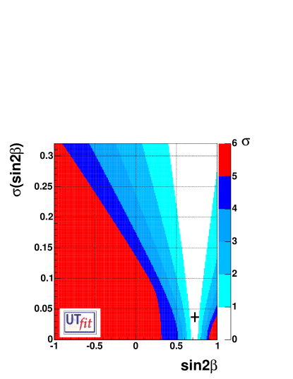
Figure 15: The compatibility (“pull”) between the direct and indirect determination of $\sin{2\beta}$ as a function of the measured values and errors. On the left, the indirect distribution of $\sin{2\beta}$ is computed from the UT fit including $|V_{ub}/V_{cb}|$, $\Delta m_{d}$, $\Delta m_{s}$, and $\varepsilon_{K}$, without using the direct measurement from $B^{0}\to J/\psi K^{0}$. On the right, the indirect distribution includes also the constraint from the measurements of $\sin{2\beta}$ from $B^{0}\to J/\psi K^{0}$. The compatibility regions from $1\sigma$ to $6\sigma$ are displayed. The crosses display the position (value/error) of the measurements of $\sin{2\beta}$ from $B^{0}\to J/\psi K^{0}$(left plot) and from $B\to\phi K^{0}$ (right plot), extracted from the HFAG average for $S(\phi K^{0})$. We also mark with an asterisk the value of $\sin{2\beta}$ obtained using instead our skeptical combination for $S(\phi K^{0})$.

The plot shows that, considering the present precision of $0.037$ on the measured value of $\sin{2\beta}$, the 3$\sigma$ compatibility region is in the range [0.51, 0.88]. Values outside this range would be, therefore, not compatible with the SM prediction at more than $3\sigma$ level. To get these values, however, the presently measured central value should shift by at least $6\sigma$.

The conclusion that can be derived from Figure 15 is the following: although the improvement on the error on sin2$\beta$ has an important impact on the accuracy of the UT parameter determination, it is very unlikely that in the near future we will be able to use this measurement to detect any failure of the SM, unless the other constraints entering the fit improve substantially or, of course, in case the central value of the direct measurement moves away from the present one by several standard deviations.

5.2.1 Rôle of $\sin{2\beta}$ from Penguin processes

It was pointed out some time ago that the comparison of the time-dependent CP asymmetries in various $B$ decay modes could provide evidence of NP in $B$ decay amplitudes [22]. Since $\sin{2\beta}$ is known from $S(J/\psi K^{0})$, a significant deviation of the time-dependent asymmetry parameters of penguin dominated channels from their expected values would indicate the presence of NP.

From this point of view, the pure penguin $b\to s\bar{s}s$ processes as $B\to\phi K^{0}$ are the cleanest probes of NP. The only SM uncertainty in the extraction of $\sin{2\beta}$ from $S(\phi K^{0})$ comes from the penguin matrix elements of current-current operators containing up-type quarks. This is expected to be small and can be estimated in a given model of hadron dynamics and constrained using the experimental data. For example, using the model of ref. [25], we obtain

$$\sin{2\beta}=\left\{\begin{array}[]{l l r}0.34\pm 0.20\pm 0.08&{\rm from~{}}S_{\phi K^{0}}=0.34\pm 0.20&{\rm(HFAG)}\\ 0.46\pm 0.28\pm 0.08&{\rm from~{}}S_{\phi K^{0}}=0.46\pm 0.28&{\rm(skeptical)}\end{array}\right.$$ (28)

In the previous equation we have used both the HFAG average for $S(\phi K^{0})$ and our estimate obtained using the skeptical approach of ref. [28] (with $\delta=0.6$ and $\lambda=1.3$). The average value of $S(\phi K^{0})$ is obtained using four measurements having $\chi^{2}/NDF$=2.6. As this result is used to find evidence for NP it has been considered that systematic uncertainties may have been underestimated, so errors have been inflated using the approach [28]. If the present discrepancy were instead due to a statistical fluctuation, it should disappear in the future and the two approaches will converge to the same result.

The compatibility of $\sin{2\beta}$ shown in the right plot of Figure 15 has been obtained using all the constraints of the standard analysis, namely $|V_{ub}/V_{cb}|$, $\Delta m_{d}$, $\Delta m_{s}$, $\varepsilon_{K}$, including $\sin{2\beta}$. The cross and star on this plot correspond to the values of $\sin{2\beta}$ in Eq. (28), extracted from the HFAG and the skeptical average respectively. Depending on the chosen average procedure, the compatibility of $\sin{2\beta}$ from $B\to\phi K^{0}$ with the indirect determination ranges from about $1\sigma$ to $2\sigma$.

The extraction of $\sin{2\beta}$ could be extended to channels receiving additional contributions from $b\to u\bar{u}s$ transitions, such as $B\to\eta^{\prime}K^{0}$, $B^{0}\to f_{0}K^{0}$ or $B\to\pi^{0}K^{0}$. However, in these cases, hadronic uncertainties are more difficult to estimate and expected to be channel-dependent. For this reason, CP asymmetries in these channels can be different and should not be naïvely averaged. A detailed analysis of these modes goes beyond the goal of this work and will be presented elsewhere.

5.3 Pull distribution for $\Delta m_{s}$

The plots in Figure 16 show the compatibility of the indirect determination of $\Delta m_{s}$ with a future determination of the same quantity, obtained using or ignoring the experimental information coming from the present bound.

Figure 16: The compatibility between the direct and indirect determination of $\Delta m_{s}$, as a function of the value of $\Delta m_{s}$($ps^{-1}$), using (left) or ignoring (right) the present experimental bound.

From the plot in Figure 16 we conclude that, once a measurement of $\Delta m_{s}$ with an expected accuracy of $\sim 1$ ps^-1 is available, a value of $\Delta m_{s}$ greater than $32$ ps^-1 would imply NP at $3\sigma$ level or more.

5.4 Pull distribution for the angles $\gamma$ and $\alpha$

Figure 17: The compatibility between the direct and indirect determination of $\gamma$ (left) and $\alpha$ (right), as a function of their measured value and corresponding uncertainty using the UTfit results. The cross displays the position (value/error) of the present measurements of $\gamma$ from charged B mesons decaying into $D^{*}K^{*}$ final states.

The left plot in Figure 17 shows the compatibility of the direct and indirect determination of $\gamma$. It can be noted that, even in case the angle $\gamma$ can be measured with a precision of $10^{\circ}$ from $B$ decays, the predicted $3\sigma$ region is still rather large, corresponding to the interval [25,/,95]^∘. Values larger than 100^∘ would clearly indicate physics beyond the Standard Model.

The present direct determination of the angle $\gamma$, being in perfect agreement with UT fit, cannot provide any evidence of NP independently of the precision of the measurement. To a lesser extent, the same conclusion can be drawn for $\alpha$, see right plot in Figure 17. Assuming again a precision of $10^{\circ}$, NP at $3\sigma$ shows up outside the range [58,/,132]^∘.

6 Conclusions

Flavour physics in the quark sector has entered its mature age. Today the Unitarity Triangle parameters are known with good precision. A crucial test has been already done: the comparison between the Unitarity Triangle parameters, as determined with quantities sensitive to the sides of the triangle (semileptonic $B$ decays and oscillations), and the measurements of CP violation in the kaon ($\epsilon_{K}$) and in the $B$ (sin2$\beta$) sectors. The agreement is “unfortunately” excellent. The Standard Model is “Standardissimo”: it is also working in the flavour sector. This test of the SM has been allowed by the impressive improvements achieved on non-perturbative methods which have been used to extract the CKM parameters.

Many $B$ decay branching ratios and CP asymmetries have been measured at $B$ factories. The outstanding result is the determination of sin 2$\beta$ from $B$ hadronic decays into charmonium-$K^{0}$ final states. On the other hand many other exclusive hadronic rare $B$ decays have been measured and constitute a gold mine for weak and hadronic physics, allowing in principle to extract different combinations of the Unitarity Triangle angles.

Besides presenting an update of the standard UTfit analysis, we have shown in this paper that new measurements at $B$ factories begin to have an impact on the overall picture of the Unitarity Triangle determination. In particular the angle $\gamma$ is today measured through charged $B$ decays into $DK$ final states within 20$\%$ accuracy and only a twofold ambiguity. In the following years the precise measurements of the UT angles will provide further tests of the Standard Model in the flavour sector to an accuracy up to the percent level.

Finally, by introducing the compatibility plots, we have studied the impact of future measurements for testing the SM and looking for new physics. In the near future the measurement of $\Delta m_{s}$ and of the UT angle $\gamma$ will play the leading rôle.

7 Acknowledgements

We would like to warmly thank people who provided us the experimental and theoretical inputs which are an essential part of this work and helped us with useful suggestions for the correct use of the experimental information. We thank: A. Bevan, T. Browder, C. Campagnari, G. Cavoto, M. Danielson, R. Faccini, F. Ferroni, P. Gambino, G. Isidori, M. Legendre, O. Long, F. Martinez, L. Roos, A. Poulenkov, M. Rama, Y. Sakai, M.-H. Schune, W. Verkerke, M. Zito. We also thank A. Soni for useful discussions. Finally, we thank M. Baldessari, C. Bulfon, and all the BaBar Rome group for help in the realization and for hosting the web site.

References

- [1] R. Barbieri, A. Pomarol, R. Rattazzi and A. Strumia, Nucl. Phys. B 703 (2004) 127 [arXiv:hep-ph/0405040].
- [2] M. Ciuchini, G. D’Agostini, E. Franco, V. Lubicz, G. Martinelli, F. Parodi, P. Roudeau, A. Stocchi, JHEP 0107 (2001) 013. (hep-ph/0012308);
-
[3]
M. Ciuchini, E. Franco, V. Lubicz, F. Parodi, L.
Silvestrini and A. Stocchi, (hep-ph/0307195);
A. J. Buras, F. Parodi, A. Stocchi, JHEP 0301 (2003) 029 (hep-ph/0207101). - [4] M. Lusignoli, L. Maiani, G. Martinelli and L. Reina, Nucl. Phys. B 369, 139 (1992); A. Ali and D. London, arXiv:hep-ph/9405283; arXiv:hep-ph/9409399; Z. Phys. C 65, 431 (1995); S. Herrlich and U. Nierste, Phys. Rev. D 52, 6505 (1995); M. Ciuchini, E. Franco, G. Martinelli, L. Reina and L. Silvestrini, Z. Phys. C 68, 239 (1995); A. Ali and D. London, Nuovo Cim. 109A, 957 (1996); A. Ali, Acta Phys. Polon. B 27, 3529 (1996); A. J. Buras, arXiv:hep-ph/9711217; A. J. Buras and R. Fleischer, Adv. Ser. Direct. High Energy Phys. 15, 65 (1998); R. Barbieri, L. J. Hall, S. Raby and A. Romanino, Nucl. Phys. B 493, 3 (1997); A. Ali and B. Kayser, arXiv:hep-ph/9806230; P. Paganini, F. Parodi, P. Roudeau and A. Stocchi, Phys. Scripta 58, 556 (1998); F. Parodi, P. Roudeau and A. Stocchi, Nuovo Cim. A 112, 833 (1999); F. Caravaglios, F. Parodi, P. Roudeau and A. Stocchi, arXiv:hep-ph/0002171; S. Mele, Phys. Rev. D 59, 113011 (1999); A. Ali and D. London, Eur. Phys. J. C 9, 687 (1999); M. Ciuchini, E. Franco, L. Giusti, V. Lubicz and G. Martinelli, Nucl. Phys. B 573, 201 (2000); M. Bargiotti et al., La Rivista del Nuovo Cimento Vol. 23N3 (2000) 1; S. Plaszczynski and M. H. Schune, arXiv:hep-ph/9911280; S. Mele, in Proc. of the 5th International Symposium on Radiative Corrections (RADCOR 2000) ed. Howard E. Haber, arXiv:hep-ph/0103040; A. Hocker, H. Lacker, S. Laplace and F. Le Diberder, Eur. Phys. J. C 21 (2001) 225; M. Ciuchini, Nucl. Phys. Proc. Suppl. 109B (2002) 307; A. Hocker, H. Lacker, S. Laplace and F. Le Diberder, AIP Conf. Proc. 618 (2002) 27; F. Caravaglios, P. Roudeau and A. Stocchi, Nucl. Phys. B 633 (2002) 193; A. J. Buras, arXiv:hep-ph/0210291; G. P. Dubois-Felsmann, D. G. Hitlin, F. C. Porter and G. Eigen, arXiv:hep-ph/0308262; arXiv:hep-ex/0312062; A. Stocchi, arXiv:hep-ph/0405038; J. Charles et al. [CKMfitter Group Collaboration], arXiv:hep-ph/0406184.
- [5] H. F. A. Group, arXiv:hep-ex/0412073; http://www.slac.stanford.edu/xorg/hfag/
- [6] V. M. Abazov et al. [D0 Collaboration], Nature 429 (2004) 638 [arXiv:hep-ex/0406031].
- [7] D. Becirevic et al., arXiv:hep-lat/0411016; F. Mescia, arXiv:hep-ph/0411097.
- [8] A. de Rujula, M. Lusignoli, M. Masetti, A. Pich, S. Petrarca, J. Prades, A. Pugliese and H. Steger, in LHC Workshop Proc., Vol II,p. 205 and Fig 3 in p. 216, CERN 90-10, ECFA 90-133, DEC. 1990; C. Dib, I. Dunietz, F. Gilman, Y. Nir, Phys. Rev. D41 (1990) 1522; G. Buchalla, A.J. Buras and M.E. Lautenbacher, Rev. Mod. Phys. 68 (1996) 1125; A. Ali and D. London, in Proceeding of “ECFA Workshop on the Physics of a Meson Factory”, Ed. R. Aleksan, A. Ali (1993); A. Ali and D. London, Nucl. Phys. 54A (1997) 297.
- [9] M. Gronau and D. London, Phys. Lett. B253, 483 (1991); M. Gronau and D. Wyler, Phys. Lett.B265, 172 (1991).
- [10] I. Dunietz, Phys. Lett. B270, 75 (1991); I. Dunietz, Z. Phys. C56, 129 (1992); D. Atwood, G. Eilam, M. Gronau and A. Soni, Phys. Lett. B341, 372 (1995); D. Atwood, I. Dunietz and A. Soni, Phys. Rev. Lett. 78, 3257 (1997).
- [11] A. Giri, Yu. Grossman, A. Soffer and J. Zupan, Phys. Rev. D68, 054018 (2003).
- [12] A. Bondar and T. Gershon, Phys. Rev. D 70 (2004) 091503 [arXiv:hep-ph/0409281].
- [13] B. Aubert et al. [BABAR Collaboration], arXiv:hep-ex/0408082; B. Aubert et al. [BABAR Collaboration], arXiv:hep-ex/0408060; B. Aubert et al. [BABAR Collaboration], arXiv:hep-ex/0408069; K. Abe et al. [BELLE Collaboration], Belle-CONF-0443; K. Abe et al. [BELLE Collaboration],arXiv:hep-ex/0307074; B. Aubert et al. [the BABAR Collaboration], arXiv:hep-ex/0408028; K. Abe et al. [Belle Collaboration],arXiv:hep-ex/0408129; B. Aubert et al. [BABAR Collaboration], arXiv:hep-ex/0408088; A. Poluektov et al. [Belle Collaboration], Phys. Rev. D 70 (2004) 072003 [arXiv:hep-ex/0406067].
- [14] Y. Grossman and H. R. Quinn, Phys. Rev. D 58 (1998) 017504 [arXiv:hep-ph/9712306]; J. Charles, Phys. Rev. D 59 (1999) 054007 [arXiv:hep-ph/9806468]; M. Gronau, D. London, N. Sinha and R. Sinha, Phys. Lett. B 514, 315 (2001) [arXiv:hep-ph/0105308]. M. Pivk and F. R. Le Diberder, arXiv:hep-ph/0406263.
- [15] M. Gronau and D. London, Phys. Rev. Lett. 65 (1990) 3381.
- [16] B. Aubert et al. [BABAR Collaboration], arXiv:hep-ex/0408089. K. Abe et al. [Belle Collaboration], Phys. Rev. Lett. 93 (2004) 021601 [arXiv:hep-ex/0401029].
- [17] A. E. Snyder and H. R. Quinn, Phys. Rev. D 48 (1993) 2139.
- [18] B. Aubert et al. [BABAR Collaboration], arXiv:hep-ex/0408099.
- [19] O. Long, M. Baak, R. N. Cahn and D. Kirkby, Phys. Rev. D 68 (2003) 034010 [arXiv:hep-ex/0303030].
- [20] B. Aubert et al. [BABAR Collaboration], Phys. Rev. Lett. 92 (2004) 251801 [arXiv:hep-ex/0308018]; B. Aubert et al. [BABAR Collaboration], Phys. Rev. Lett. 92 (2004) 251802 [arXiv:hep-ex/0310037]; B. Aubert et al. [BABAR Collaboration],arXiv:hep-ex/0408038; B. Aubert et al. [BABAR Collaboration],arXiv:hep-ex/0408059; K. Abe et al. [BELLE Collaboration], arXiv:hep-ex/0408106. K. Abe et al. [BELLE Collaboration], Phys. Rev. Lett. 93 (2004) 031802 [Erratum-ibid. 93 (2004) 059901] [arXiv:hep-ex/0308048].
- [21] R. Aleksan and T. C. Petersen, eConf C0304052 (2003) WG414 [arXiv:hep-ph/0307371].
- [22] Y. Grossman and M. P. Worah, Phys. Lett. B 395 (1997) 241 [arXiv:hep-ph/9612269]; M. Ciuchini, E. Franco, G. Martinelli, A. Masiero and L. Silvestrini, Phys. Rev. Lett. 79 (1997) 978 [arXiv:hep-ph/9704274]; Y. Grossman, G. Isidori and M. P. Worah, Phys. Rev. D 58 (1998) 057504 [arXiv:hep-ph/9708305].
- [23] A. J. Buras and L. Silvestrini, Nucl. Phys. B 569 (2000) 3 [arXiv:hep-ph/9812392].
- [24] B. Aubert et al. [BABAR Collaboration], Phys. Rev. Lett. 93 (2004) 071801 [arXiv:hep-ex/0403026]; K. Abe et al. [Belle Collaboration], Phys. Rev. Lett. 91 (2003) 261602 [arXiv:hep-ex/0308035]; B. Aubert et al. [BABAR Collaboration], Phys. Rev. Lett. 93 (2004) 131805 [arXiv:hep-ex/0403001].
- [25] M. Ciuchini, E. Franco, G. Martinelli, M. Pierini and L. Silvestrini, Phys. Lett. B 515 (2001) 33 [arXiv:hep-ph/0104126]; M. Ciuchini, E. Franco, G. Martinelli, A. Masiero, M. Pierini and L. Silvestrini, arXiv:hep-ph/0407073.
- [26] M. Ciuchini, E. Franco, F. Parodi, V. Lubicz, L. Silvestrini and A. Stocchi, eConf C0304052 (2003) WG306 [arXiv:hep-ph/0307195].
- [27] P.F. Harrison and H.R. Quinn [BaBar Collaboration], SLAC-R-0504.
- [28] G. D’Agostini hep-ex/9910036.