The role of Cahn and Sivers effects in Deep Inelastic Scattering

Abstract

The role of intrinsic $\mbox{\boldmath$k$}_{\perp}$ in inclusive and semi-inclusive Deep Inelastic Scattering processes ($\ell\,p\to\ell\,h\,X$) is studied with exact kinematics within QCD parton model at leading order; the dependence of the unpolarized cross section on the azimuthal angle between the leptonic and the hadron production planes (Cahn effect) is compared with data and used to estimate the average values of $k_{\perp}$ both in quark distribution and fragmentation functions. The resulting picture is applied to the description of the weighted single spin asymmetry $A_{UT}^{\sin(\phi_{\pi}-\phi_{S})}$ recently measured by the HERMES collaboration at DESY; this allows to extract some simple models for the quark Sivers functions. These are compared with the Sivers functions which succeed in describing the data on transverse single spin asymmetries in $p^{\uparrow}\,p\to\pi\,X$ processes; the two sets of functions are not inconsistent. The extracted Sivers functions give predictions for the COMPASS measurement of $A_{UT}^{\sin(\phi_{\pi}-\phi_{S})}$ in agreement with recent preliminary data, while their contribution to HERMES $A_{UL}^{\sin\phi_{\pi}}$ is computed and found to be small. Predictions for $A_{UT}^{\sin(\phi_{K}-\phi_{S})}$ for kaon production at HERMES are also given.

I Introduction

It is becoming increasingly clear that unintegrated parton distribution and fragmentation functions play a significant role in many physical processes and that they are more fundamental objects than the usual integrated versions; intrinsic $\mbox{\boldmath$k$}_{\perp}$ originates both from partonic confinement and from basic QCD evolution ab and often cannot be ignored in perturbative QCD hard processes and in soft non perturbative physics. For example, this was already pointed out in Refs. fff concerning the computation of the unpolarized cross section for inclusive hard scattering processes like $p\,p\to h\,X$ at intermediate energy values. Similarly, in semi-inclusive Deep Inelastic Scattering (SIDIS) processes, $\ell\,p\to\ell\,h\,X$, the intrinsic partonic motion results in an azimuthal dependence of the produced hadron $h$ cahn ; kk ; EMC1 ; EMC2 . A full consistent treatment of several inclusive $p\,p$ processes with all intrinsic motions, in different kinematical regions, has been recently discussed in Ref. fu .

While the role of intrinsic $\mbox{\boldmath$k$}_{\perp}$ can be important in unpolarized processes, it becomes crucial for the explanation of many single spin effects recently observed and still under active investigation in several ongoing experiments; spin and $\mbox{\boldmath$k$}_{\perp}$ dependences can couple in parton distributions and fragmentations rev , thus giving origin to unexpected effects in polarization observables. One such example is the azimuthal asymmetry observed by the HERMES collaboration in the scattering of unpolarized leptons off polarized protons hermUL ; hermUT . Another striking case is the observation of large transverse single spin asymmetries (SSA) in $p^{\uparrow}\,p\to\pi\,X$ processes e704 ; star .

We consider here in a consistent approach the role of parton intrinsic motion in inclusive and semi-inclusive DIS processes within QCD parton model at leading order; the kinematics of intrinsic $\mbox{\boldmath$k$}_{\perp}$ is fully taken into account in quark distribution functions, in the elementary processes and in the quark fragmentation process. This induces several corrections of order $k_{\perp}/Q$ or higher, which are exactly computed: however, we do not consider similar corrections which might originate from higher-twist distribution and fragmentation functions mt . The average values of $k_{\perp}$ for quarks inside protons, and for final hadrons inside the fragmenting quark jet, are fixed by a comparison with data on the dependence of the unpolarized cross section on the azimuthal angle between the leptonic and the hadronic planes.

Such values are then used to compute the SSA for $\ell\,p^{\uparrow}\to\ell\,\pi\,X$ processes, which would be zero without any intrinsic motion. We concentrate on the Sivers mechanism siv , that is the spin and $\mbox{\boldmath$k$}_{\perp}$ dependence in the distribution of unpolarized quarks inside a transversely polarized proton; it can be isolated by studying the weighted SSA $A_{UT}^{\sin(\phi_{\pi}-\phi_{S})}$ bm , recently measured by HERMES hermUT and, still preliminarily, by COMPASS compUT collaborations. Although the data are still scarce, with large errors, a first qualitative estimate of the quark Sivers functions can be obtained; the information gathered from HERMES data is in agreement with the preliminary COMPASS data. The contribution of these functions to the weighted longitudinal SSA $A_{UL}^{\sin\phi_{\pi}}$ is computed and shown to be negligible: the measured $A_{UL}^{\sin\phi_{\pi}}$ hermUL can be equally originated not only by the Sivers mechanism, but also by the Collins effect col , occurring in the fragmentation of a transversely polarized quark, and by higher-twist contributions.

A similar analysis of SSA in $p^{\uparrow}\,p\to\pi\,X$ processes, with a separate study of the Sivers and the Collins contributions, has been performed respectively in Refs. fu and noicol , with the conclusion that the Sivers mechanism alone can explain the data e704 , while the Collins mechanism is strongly suppressed. Explicit expressions of the quark Sivers functions, as obtained from data on SSA in $p^{\uparrow}\,p\to\pi\,X$ processes, are given in ref. fu . They are qualitatively similar to the Sivers functions obtained here from SIDIS processes. Let us notice that the universality of the Sivers function is an important open issue; it has been proven that the quark Sivers functions in SIDIS and in Drell-Yan processes must be opposite colsdy , while no definite conclusion has been theoretically reached concerning the relation between the Sivers function in SIDIS and $pp$ processes cm .

II Definitions and kinematics

Let us start from the kinematics of Deep Inelastic Scattering processes in the $\gamma^{*}p$ c.m. frame, as shown in Fig. 1. We take the photon and the proton colliding along the $z$ axis with momenta $q$ and $P$ respectively; the leptonic plane coincides with the $x$-$z$ plane (following the so-called “Trento conventions” trento ). We adopt the usual DIS variables (neglecting the lepton mass):

$$s=(P+\ell)^{2}\quad\quad Q^{2}=-q^{2}\quad\quad(P+q)^{2}=W^{2}=\frac{1-x_{\!\scriptscriptstyle B}}{x_{\!\scriptscriptstyle B}}\,Q^{2}+m_{p}^{2}$$

$$x_{\!\scriptscriptstyle B}=\frac{Q^{2}}{2P\cdot q}=\frac{Q^{2}}{W^{2}+Q^{2}-m_{p}^{2}}\quad\quad y=\frac{P\cdot q}{P\cdot\ell}=\frac{Q^{2}}{x_{\!\scriptscriptstyle B}(s-m_{p}^{2})}\>\cdot$$ (1)

Figure 1: Kinematics of DIS processes.

If one neglects also the proton mass $m_{p}$ the four-momenta involved can be written as:

$$\ell = E(1,\sin\theta,0,\cos\theta)=(E,\mbox{\boldmath$\ell$})$$

$$\ell^{\prime} = \ell-q$$

$$q = \frac{1}{2}\left(W-\frac{Q^{2}}{W},0,0,W+\frac{Q^{2}}{W}\right)$$

$$P = P_{0}(1,0,0,-1)\;,$$

where

$$\cos\theta=\frac{Q^{2}+E(W-Q^{2}/W)}{E(W+Q^{2}/W)}=\frac{1+(y-2)\,x_{\!\scriptscriptstyle B}}{1-y\,x_{\!\scriptscriptstyle B}}$$

$$\quad\quad E=\frac{s-Q^{2}}{2W}\quad\quad P_{0}=\frac{1}{2}\left(W+\frac{Q^{2}}{W}\right)\>\cdot$$ (2)

At leading QCD order the lepton scatters off a quark and, taking intrinsic motion into account, the initial and final quark four-momenta are given by:

$$k=\left(xP_{0}+\frac{k_{\perp}^{2}}{4xP_{0}},\,\mbox{\boldmath$k$}_{\perp},\,-xP_{0}+\frac{k_{\perp}^{2}}{4xP_{0}}\right)\quad\quad\quad k^{\prime}=k+q$$ (3)

where $x=k^{-}/P^{-}$ is the light-cone fraction of the proton momentum carried by the parton and $\mbox{\boldmath$k$}_{\perp}=k_{\perp}(\cos\varphi,\sin\varphi,0)$ is the parton transverse momentum, with $k_{\perp}\equiv|\mbox{\boldmath$k$}_{\perp}|$.

The elementary Mandelstam variables $\hat{s}=(l+k)^{2}$, $\hat{t}=(l-l^{\prime})^{2}$, and $\hat{u}=(k-l^{\prime})^{2}$ are then given by:

$$\hat{s} = xs-2\mbox{\boldmath$\ell$}\cdot\mbox{\boldmath$k$}_{\perp}-k_{\perp}^{2}\frac{x_{\!\scriptscriptstyle B}}{x}\left(1-\frac{x_{\!\scriptscriptstyle B}s}{Q^{2}}\right)$$

$$\hat{t} = -Q^{2}$$ (4)

$$\hat{u} = -x\left(s-\frac{Q^{2}}{x_{\!\scriptscriptstyle B}}\right)+2\mbox{\boldmath$\ell$}\cdot\mbox{\boldmath$k$}_{\perp}-k_{\perp}^{2}\frac{x_{\!\scriptscriptstyle B}^{2}s}{xQ^{2}}\>\cdot$$

The on-shell condition for the final quark

$$k^{\prime 2}=2q\cdot k-Q^{2}=\hat{s}+\hat{t}+\hat{u}=0$$ (5)

implies

$$x=\frac{1}{2}\,x_{\!\scriptscriptstyle B}\left(1+\sqrt{1+\frac{4k_{\perp}^{2}}{Q^{2}}}\right)\cdot$$ (6)

Notice that when terms ${\cal O}(k_{\perp}^{2}/Q^{2})$ are neglected in the above equations one recovers the usual relations $x=x_{\!\scriptscriptstyle B}$ and $\mbox{\boldmath$k$}=x_{\!\scriptscriptstyle B}\mbox{\boldmath$P$}+\mbox{\boldmath$k$}_{\perp}$; however, a significant dependence on the azimuthal angle $\varphi$ remains, at ${\cal O}(k_{\perp}/Q)$, in the partonic Mandelstam invariants $\hat{s}$ and $\hat{u}$, via

$$\mbox{\boldmath$\ell$}\cdot\mbox{\boldmath$k$}_{\perp}=Ek_{\perp}\,\sin\theta\,\cos\varphi\>.$$ (7)

One explicitly has

$$\hat{s}^{2} = \frac{Q^{4}}{y^{2}}\left[1-4\frac{k_{\perp}}{Q}\,\sqrt{1-y}\,\cos\varphi\right]+{\cal O}\left(\frac{k_{\perp}^{2}}{Q^{2}}\right)$$ (8)

$$\hat{u}^{2} = \frac{Q^{4}}{y^{2}}\,(1-y)^{2}\left[1-4\frac{k_{\perp}}{Q}\,\frac{\cos\varphi}{\sqrt{1-y}}\right]+{\cal O}\left(\frac{k_{\perp}^{2}}{Q^{2}}\right)\cdot$$ (9)

II.1 DIS cross section

Let us recall the expression of the cross section for Deep Inelastic Scattering processes, $\ell\,p\to\ell\,X$, in the framework of the QCD parton model with the inclusion of intrinsic $\mbox{\boldmath$k$}_{\perp}$ lp ; aram . One starts from

$$\frac{d^{2}\sigma^{\ell p\to\ell X}}{dx_{\!\scriptscriptstyle B}\,dQ^{2}}=\frac{\pi\alpha^{2}}{Q^{2}}\frac{1}{x_{\!\scriptscriptstyle B}^{2}\,s^{2}}\,L_{\mu\nu}W^{\mu\nu}\;,$$ (10)

with

$$L_{\mu\nu}=2(l_{\mu}l^{\prime}_{\nu}+l^{\prime}_{\mu}l_{\nu}-g_{\mu\nu}\,l\cdot l^{\prime})\;,$$ (11)

and

$$W^{\mu\nu}=\sum_{q}\int dx\,d^{2}\mbox{\boldmath$k$}_{\perp}\left(\frac{1}{x}\right)f_{q}(x,k_{\perp})\,w^{\mu\nu}\;,$$ (12)

where $f_{q}(x,k_{\perp})$ is the number density of quarks of flavor $q$ inside the initial hadron, carrying a transverse momentum $\mbox{\boldmath$k$}_{\perp}$ and a light-cone fraction $x$ of the proton momentum. The elementary quark tensor is given by

$$w_{\mu\nu}=2e_{q}^{2}\left(k_{\mu}k^{\prime}_{\nu}+k^{\prime}_{\mu}k_{\nu}-g_{\mu\nu}\frac{Q^{2}}{2}\right)\delta(2q\cdot k-Q^{2})\;,$$ (13)

so that

$$L_{\mu\nu}\,w^{\mu\nu}=2\,e_{q}^{2}\,\delta(2q\cdot k-Q^{2})\,(\hat{s}^{2}+\hat{u}^{2})\>.$$ (14)

In the collinear case, $f_{q}(x,k_{\perp})=f_{q}(x)\,\delta^{2}(\mbox{\boldmath$k$}_{\perp})$, Eqs. (10)–(14) simply result into

$$\frac{d^{2}\sigma^{\ell p\to\ell X}}{dx_{\!\scriptscriptstyle B}\,dQ^{2}}=\sum_{q}f_{q}(x_{\!\scriptscriptstyle B})\frac{d\hat{\sigma}^{\ell q\to\ell q}}{dQ^{2}}\;,$$ (15)

where $d\hat{\sigma}^{lq\to lq}$ is the cross section for the elementary lepton-quark scattering,

$$\frac{d\hat{\sigma}^{\ell q\to\ell q}}{dQ^{2}}=e_{q}^{2}\,\frac{2\pi\alpha^{2}}{x_{\!\scriptscriptstyle B}^{2}s^{2}}\,\frac{\hat{s}^{2}+\hat{u}^{2}}{Q^{4}}\;\cdot$$ (16)

In the general non collinear case one obtains instead:

$$\frac{d^{2}\sigma^{\ell p\to\ell X}}{dx_{\!\scriptscriptstyle B}\,dQ^{2}}=\sum_{q}\int{d^{2}\mbox{\boldmath$k$}_{\perp}}\;f_{q}(x,k_{\perp})\;\frac{d\hat{\sigma}^{\ell q\to\ell q}}{dQ^{2}}\;J(x_{\!\scriptscriptstyle B},Q^{2},\mbox{\boldmath$k$}_{\perp})\>,$$ (17)

where $x$ is given in Eq. (6) and the function $J$ is given by

$$J=\frac{x_{\!\scriptscriptstyle B}}{x}\left(1+\frac{x_{\!\scriptscriptstyle B}^{2}}{x^{2}}\frac{k_{\perp}^{2}}{Q^{2}}\right)^{\!\!-1}\cdot$$ (18)

Notice that $J=1$ in the collinear case; the elementary $d\hat{\sigma}$ in Eq. (17) is the same as in Eq. (16) with the Mandelstam variables of Eqs. (4), which depend on $\mbox{\boldmath$k$}_{\perp}$.

If one could detect the final quark – for example by reconstructing the current fragmentation jet – the DIS cross section could be written as

$$\frac{d^{4}\sigma^{\ell p\to\ell+jet+X}}{dx_{\!\scriptscriptstyle B}\,dQ^{2}\,d^{2}\mbox{\boldmath$k$}_{\perp}}=\sum_{q}f_{q}(x,k_{\perp})\;\frac{d\hat{\sigma}^{\ell q\to\ell q}}{dQ^{2}}\,J(x_{\!\scriptscriptstyle B},Q^{2},k_{\perp})\>,$$ (19)

and one could test the azimuthal dependence of the cross section on the angle $\varphi$ between the leptonic and the jet plane, Fig. 1. Such a dependence, resulting from $\hat{s}^{2}+\hat{u}^{2}$, Eqs. (8) and (9), was suggested by Cahn cahn , in semi-inclusive DIS, assuming that the fragmentation process $q\to hX$ is essentially collinear and the direction of the final detected hadron is close to that of the quark. Smearing effects due to the fragmentation process were also taken into account cahn ; kk ; aram . In the next subsection we shall consider SIDIS processes, fully taking into account the intrinsic motion and the angular dependence in the fragmentation process; we shall see that indeed a dependence on an azimuthal angle remains, which allows to obtain an estimate of the average transverse momentum in distribution and fragmentation functions.

II.2 SIDIS cross section

Let us consider semi-inclusive DIS processes, $\ell\,p\to\ell\,h\,X$, in the $\gamma^{*}p$ c.m. frame and in the kinematic regime in which $P_{T}\simeq\Lambda_{\rm QCD}\simeq k_{\perp}$, where $P_{T}=|\mbox{\boldmath$P$}_{T}|$ is the final hadron transverse momentum. In this region leading order elementary processes, $\ell\,q\to\ell\,q$, are dominating: the soft $P_{T}$ of the detected hadron is mainly originating from quark intrinsic motion EMC1 ; EMC2 ; E665 , rather than from higher order pQCD interactions, which, instead, would dominantly produce large $P_{T}$ hadrons ces ; nlo ; dfs .

We adopt as our starting point a factorized scheme, introducing – within the leading-order parton model with leading-twist distribution and fragmentation functions – the exact $k_{\perp}$ kinematics; this induces corrections of the ${\cal O}(k_{\perp}/Q)$ or higher, which we wish to explore and compare with experiments. A formal QCD factorization, in the same low transverse momentum region and at leading order in $k_{\perp}/Q$, has been recently proved ji .

In the factorization scheme, assuming an independent fragmentation process, the SIDIS cross section for the production of a hadron $h$ inside the jet originated from a final quark with transverse momentum $\mbox{\boldmath$k$}_{\perp}$ can be written as

$$\frac{d^{7}\sigma^{\ell p\to\ell+jet+h+X}}{dx_{\!\scriptscriptstyle B}\,dQ^{2}\,d^{2}\mbox{\boldmath$k$}_{\perp}\,dz\,d^{2}\mbox{\boldmath$p$}_{\perp}}=\sum_{q}\>f_{q}(x,k_{\perp})\;\frac{d\hat{\sigma}^{\ell q\to\ell q}}{dQ^{2}}\;J(x_{\!\scriptscriptstyle B},Q^{2},k_{\perp})\;D_{q}^{h}(z,p_{\perp})\,,$$ (20)

where $D_{q}^{h}(z,\mbox{\boldmath$p$}_{\perp})$ is the number density of hadrons $h$ resulting from the fragmentation of the final parton $q$, normalized so that

$$\int\!dz\,d^{2}\mbox{\boldmath$p$}_{\perp}\,D_{q}^{h}(z,p_{\perp})=\langle N_{h}\rangle\,,$$ (21)

where $\langle N_{h}\rangle$ is the average multiplicity of hadron $h$ in the current fragmentation region of quark $q$ and

$$\int\!d^{2}\mbox{\boldmath$p$}_{\perp}\,D_{q}^{h}(z,p_{\perp})=D_{q}^{h}(z)\,.$$ (22)

$\mbox{\boldmath$p$}_{\perp}$ is the transverse momentum of the hadron $h$ with respect to the direction $\mbox{\boldmath$k$}^{\prime}$ of the fragmenting quark and $z=P_{h}^{+}/k^{+}$ is the light-cone fraction of the quark momentum carried by the resulting hadron in the ($\tilde{x},\tilde{y},\tilde{z}$)–system (see Figs. 2 and 3). These natural variables for the fragmentation process can be written as:

$$z = \frac{P_{h}^{0}+\mbox{\boldmath$P$}_{h}\cdot\hat{\mbox{\boldmath$k$}}^{\prime}}{2{k^{\prime}}^{0}}$$ (23)

$$\mbox{\boldmath$p$}_{\perp} = \mbox{\boldmath$P$}_{h}-(\mbox{\boldmath$P$}_{h}\cdot\hat{\mbox{\boldmath$k$}}^{\prime})\,\hat{\mbox{\boldmath$k$}}^{\prime}\,,$$ (24)

where $P_{h}=(P_{h}^{0},\mbox{\boldmath$P$}_{T},P_{h}^{3})$ and $k^{\prime}=k+q=({k^{\prime}}^{0},\mbox{\boldmath$k$}_{\perp},k^{\prime 3})$, with:

$${k^{\prime}}^{0} = \frac{W}{2}\left(\frac{x-2x_{\!\scriptscriptstyle B}+1}{1-x_{\!\scriptscriptstyle B}}+\frac{x_{\!\scriptscriptstyle B}}{x}\,\frac{k_{\perp}^{2}}{Q^{2}}\right)$$

$$k^{\prime 3} = \frac{W}{2}\left(\frac{1-x}{1-x_{\!\scriptscriptstyle B}}+\frac{x_{\!\scriptscriptstyle B}}{x}\,\frac{k_{\perp}^{2}}{Q^{2}}\right)$$ (25)

$$|\mbox{\boldmath$k$}^{\prime}|^{2} = k_{\perp}^{2}+(k^{\prime 3})^{2}\,.$$

Figure 2: Kinematics of the fragmentation process.

The above equations allow us to express, for each value of $x_{\!\scriptscriptstyle B}$ and $Q^{2}$, the fragmentation variables $z$ and $\mbox{\boldmath$p$}_{\perp}$ in terms of the usual observed hadronic variables $\mbox{\boldmath$P$}_{T}$ and $z_{h}=(P\cdot P_{h})/(P\cdot q)=(P_{h}^{0}+P_{h}^{3})/W$. One finds

$$z = \frac{1}{2{k^{\prime}}^{0}}\left[\left(\frac{z_{h}\,W}{2}+\frac{P_{T}^{2}}{2z_{h}\,W}\right)+\frac{\mbox{\boldmath$P$}_{T}\cdot\mbox{\boldmath$k$}_{\perp}}{|\mbox{\boldmath$k$}^{\prime}|}+\frac{k^{\prime 3}}{|\mbox{\boldmath$k$}^{\prime}|}\left(\frac{z_{h}\,W}{2}-\frac{P_{T}^{2}}{2z_{h}\,W}\right)\right]$$ (26)

$$= z_{h}+\frac{k_{\perp}P_{T}}{Q^{2}}\frac{2x_{\!\scriptscriptstyle B}}{1-x_{\!\scriptscriptstyle B}}\,\cos(\phi_{h}-\varphi)+{\cal O}\left(\frac{k_{\perp}^{2}}{Q^{2}}\right)=z_{h}+{\cal O}\left(\frac{k_{\perp}^{2}}{Q^{2}}\right)$$ (27)

and

$$\mbox{\boldmath$p$}_{\perp} = \left(\mbox{\boldmath$P$}_{T}-\frac{\mbox{\boldmath$P$}_{T}\cdot\mbox{\boldmath$k$}_{\perp}+P_{h}^{3}k^{\prime 3}}{|\mbox{\boldmath$k$}^{\prime}|^{2}}\,\mbox{\boldmath$k$}_{\perp}\,,\;P_{h}^{3}-\frac{\mbox{\boldmath$P$}_{T}\cdot\mbox{\boldmath$k$}_{\perp}+P_{h}^{3}k^{\prime 3}}{|\mbox{\boldmath$k$}^{\prime}|^{2}}\,k^{\prime 3}\right)$$ (28)

$$= \mbox{\boldmath$P$}_{T}-z_{h}\,\mbox{\boldmath$k$}_{\perp}+{\cal O}\left(\frac{k_{\perp}^{2}}{Q^{2}}\right)$$ (29)

where $k^{\prime 0},k^{\prime 3}$ and $|\mbox{\boldmath$k$}^{\prime}|$ are given in Eqs. (25) and $P_{h}^{3}=(z_{h}\,W)/2-P_{T}^{2}/(2z_{h}\,W)$.

Figure 3: Three dimensional kinematics of the SIDIS process.

Eqs. (26) and (28) allow us to describe the fragmentation process in terms of the variables $(z_{h},\mbox{\boldmath$P$}_{T})$:

$$dz\;d^{2}\mbox{\boldmath$p$}_{\perp}=dz_{h}\;d^{2}\mbox{\boldmath$P$}_{T}\;\frac{z}{z_{h}}\>,$$ (30)

so that, finally, the SIDIS cross section (20) can be written in terms of physical observables as:

$$\frac{d^{5}\sigma^{\ell p\to\ell hX}}{dx_{\!\scriptscriptstyle B}\,dQ^{2}\,dz_{h}\,d^{2}\mbox{\boldmath$P$}_{T}}=\sum_{q}\int{d^{2}\mbox{\boldmath$k$}_{\perp}}\;f_{q}(x,k_{\perp})\;\frac{d\hat{\sigma}^{\ell q\to\ell q}}{dQ^{2}}\;J\;\frac{z}{z_{h}}\;D_{q}^{h}(z,p_{\perp})$$ (31)

$$\hskip 11.38092pt=\sum_{q}e_{q}^{2}\int\!d^{2}\mbox{\boldmath$k$}_{\perp}\;f_{q}(x,k_{\perp})\;\frac{2\pi\alpha^{2}}{x_{\!\scriptscriptstyle B}^{2}s^{2}}\,\frac{\hat{s}^{2}+\hat{u}^{2}}{Q^{4}}\;D_{q}^{h}(z,p_{\perp})\;\frac{z}{z_{h}}\,\frac{x_{\!\scriptscriptstyle B}}{x}\left(1+\frac{x_{\!\scriptscriptstyle B}^{2}}{x^{2}}\frac{k_{\perp}^{2}}{Q^{2}}\right)^{\!\!-1}\>\cdot$$

This is an exact expression at all orders in $(k_{\perp}/Q)$; $x$ is given in Eq. (6) and the full expressions of $z$ and $\mbox{\boldmath$p$}_{T}$ in terms of $x_{\!\scriptscriptstyle B},Q^{2},\mbox{\boldmath$k$}_{\perp},z_{h}$ and $\mbox{\boldmath$P$}_{T}$ can be derived from Eqs. (25), (26) and (28). Notice that, in the physical variables $x_{\!\scriptscriptstyle B}$ and $z_{h}$, the $x-z$ factorization of Eq. (20) is lost, even in our simple parton model treatment; it can be recovered at ${\cal O}(k_{\perp}/Q)$ (see Eq. (32) below).

Let us now consider again the issue discussed at the end of Section II.1, concerning the azimuthal dependence of the cross section, by comparing Eqs. (19) and (31). The former equation describes the cross section for jet production and depends, as we explained, on the azimuthal angle $\varphi$, that is on the azimuthal angle of the intrinsic $\mbox{\boldmath$k$}_{\perp}$ of the quark in the proton. Such a dependence is integrated over in Eq. (31), which describes the cross section for the production of a hadron, resulting from the non collinear fragmentation of the quark. Therefore, there cannot be any $\varphi$ dependence in this cross section. However, due to relations (26) and (28), the integration over $\mbox{\boldmath$k$}_{\perp}$ at fixed $\mbox{\boldmath$P$}_{T}=P_{T}(\cos\phi_{h},\sin\phi_{h},0)$ introduces a dependence on the azimuthal angle $\phi_{h}$ of the produced hadron $h$, that is the angle between the leptonic and the hadronic plane, Fig. 3. This azimuthal dependence remains in the SIDIS cross section and will be studied in the next Section (see also Appendix A).

It is instructive, and often quite accurate, to consider the above equations in the much simpler limit in which only terms of ${\cal O}(k_{\perp}/Q)$ are retained. In such a case $x\simeq x_{\!\scriptscriptstyle B},z\simeq z_{h}$ and one obtains:

$$\frac{d^{5}\sigma^{\ell p\to\ell hX}}{dx_{\!\scriptscriptstyle B}\,dQ^{2}\,dz_{h}\,d^{2}\mbox{\boldmath$P$}_{T}}\simeq\sum_{q}e_{q}^{2}\int\!d^{2}\mbox{\boldmath$k$}_{\perp}\;f_{q}(x_{\!\scriptscriptstyle B},k_{\perp})\;\frac{2\pi\alpha^{2}}{x_{\!\scriptscriptstyle B}^{2}s^{2}}\,\frac{\hat{s}^{2}+\hat{u}^{2}}{Q^{4}}\;D_{q}^{h}(z_{h},p_{\perp})\>,$$ (32)

where $\mbox{\boldmath$p$}_{\perp}\simeq\mbox{\boldmath$P$}_{T}-z_{h}\,\mbox{\boldmath$k$}_{\perp}$, Eq. (29), and

$$\hat{s}^{2}+\hat{u}^{2}\simeq x_{\!\scriptscriptstyle B}^{2}s^{2}+(x_{\!\scriptscriptstyle B}s+Q^{2})^{2}-4\mbox{\boldmath$\ell$}\cdot\mbox{\boldmath$k$}_{\perp}(2x_{\!\scriptscriptstyle B}s-Q^{2})=$$

$$\frac{Q^{4}}{y^{2}}\left(1+(1-y)^{2}-4\frac{k_{\perp}}{Q}(2-y)\sqrt{1-y}\cos\varphi\right)\>.$$ (33)

In what follows we assume, both for the parton densities and the fragmentation functions, the usual factorization between the intrinsic transverse momentum and the light-cone fraction dependences, with a Gaussian $k_{\perp}$ dependence, that is:

$$f_{q}(x,k_{\perp})=f_{q}(x)\,\frac{1}{\pi\langle k_{\perp}^{2}\rangle}\,e^{-{k_{\perp}^{2}}/{\langle k_{\perp}^{2}\rangle}}$$ (34)

and

$$D_{q}^{h}(z,p_{\perp})=D_{q}^{h}(z)\,\frac{1}{\pi\langle p_{\perp}^{2}\rangle}\,e^{-p_{\perp}^{2}/\langle p_{\perp}^{2}\rangle}$$ (35)

so that

$$\int d^{2}\mbox{\boldmath$k$}_{\perp}\>f_{q}(x,k_{\perp})=f_{q}(x)$$ (36)

and

$$\int d^{2}\mbox{\boldmath$p$}_{\perp}\>D_{q}^{h}(z,p_{\perp})=D_{q}^{h}(z)\>.$$ (37)

With the above expressions of $f_{q}(x,k_{\perp})$ and $D_{q}^{h}(z,p_{\perp})$ the $d^{2}\mbox{\boldmath$k$}_{\perp}$ integration in Eq. (32) can be performed analytically, with the result, valid up to ${\cal O}(k_{\perp}/Q)$:

$$\frac{d^{5}\sigma^{\ell p\to\ell hX}}{dx_{\!\scriptscriptstyle B}\,dQ^{2}\,dz_{h}\,d^{2}\mbox{\boldmath$P$}_{T}}\simeq\sum_{q}\frac{2\pi\alpha^{2}e_{q}^{2}}{Q^{4}}\>f_{q}(x_{\!\scriptscriptstyle B})\>D_{q}^{h}(z_{h})\biggl{[}1+(1-y)^{2}$$

$$\hskip 36.0pt-4\>\frac{(2-y)\sqrt{1-y}\>\langle k_{\perp}^{2}\rangle\,z_{h}\,P_{T}}{\langle P_{T}^{2}\rangle\,Q}\>\cos\phi_{h}\biggr{]}\frac{1}{\pi\langle P_{T}^{2}\rangle}\,e^{-P_{T}^{2}/\langle P_{T}^{2}\rangle}\,,$$ (38)

where

$$\langle P_{T}^{2}\rangle=\langle p_{\perp}^{2}\rangle+z_{h}^{2}\langle k_{\perp}^{2}\rangle\,.$$ (39)

This approximate result illustrates very clearly the origin of the dependence of the unpolarized SIDIS cross section on the azimuthal angle $\phi_{h}$. As observed first by Cahn cahn ; aram , such a dependence is related to the parton intrinsic motion and it vanishes when $k_{\perp}=0$. Having also taken into account the intrinsic motion in the fragmentation process, Eq. (38) also depends on $\langle p_{\perp}^{2}\rangle$, via the quantity $\langle P_{T}^{2}\rangle$ defined in Eq. (39).

As we said, the above results hold in the small $P_{T}\simeq\Lambda_{\rm QCD}\simeq k_{\perp}$ region, where corrections ${\cal O}(k_{\perp}^{2}/Q^{2})$ are expected to be small. As we shall see in the next Section the numerical results obtained from Eq. (31) or from Eq. (38) are indeed very close.

III Cahn effect in unpolarized SIDIS

We wish to obtain experimental information on the average intrinsic motions. Our strategy is that of trying to describe several sets of experimental data, which explicitly measure the dependence of the SIDIS unpolarized cross section on the azimuthal angle $\phi_{h}$ between the lepton plane and the hadron production plane, and on the transverse momentum of the detected hadron $P_{T}$ (see Fig. 3); we do that by exploiting Eq. (31) or (38) and by fixing the values of $\langle k_{\perp}^{2}\rangle$ and $\langle p_{\perp}^{2}\rangle$ which best describe the data.

The $\phi_{h}$ dependence of the SIDIS cross section, for the production of charged hadrons, has been extensively studied by the EMC collaboration in the scattering of $280$ GeV muons against a hydrogen target EMC1 ; EMC2 . The shape of the differential cross section

$$\frac{d\sigma^{\ell p\to\ell hX}}{d\phi_{h}}=\int\!dx_{\!\scriptscriptstyle B}\,dQ^{2}\,dz_{h}\,P_{T}\,dP_{T}\;\frac{d^{5}\sigma^{\ell p\to\ell hX}}{dx_{\!\scriptscriptstyle B}\,dQ^{2}\,dz_{h}\,d^{2}\mbox{\boldmath$P$}_{T}}$$ (40)

is studied as a function of $\phi_{h}$.

The integration covers the $x_{\!\scriptscriptstyle B},Q^{2},z_{h}$ and $P_{T}$ regions consistent with the experimental cuts EMC2 :

$$x_{F}>0.1\quad\quad P_{T}>0.2\;{\rm GeV}/c\quad\quad y<0.8\quad\quad Q^{2}>4\;({\rm GeV}/c)^{2}\,,$$

where $x_{F}={2P_{L}}/{W}\,$ and $P_{L}$ is the longitudinal momentum of the produced hadron relative to the virtual photon, according to Fig. 3.

In our analysis we adopt the MRST 2001 (LO) MRST01 parton density functions and the fragmentation functions into charged hadrons from Ref. Kretzer .

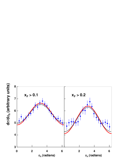
Figure 4: Fits to the $\cos\phi_{h}$ dependence of the cross section: the dashed line is obtained with exact kinematics, while the solid bold line includes terms up to ${\cal O}({k_{\perp}}/{Q})$ only. The data are from Ref. EMC2 .

Fig. 4 shows our fits to two sets of data EMC2 , corresponding to two different ranges of $x_{F}$. The solid bold line shows the result we obtain by taking into account only ${\cal O}(k_{\perp}/Q)$ contributions, Eq. (38), whereas the dashed line corresponds to the exact result at all orders in $k_{\perp}/Q$, Eq. (31). The $(-\cos\phi_{h})$ behaviour, explicit in Eq. (38), is indeed shown by the data. A possible positive contribution from a $\cos(2\phi_{h})$ term seems to be visible at small values of $\phi_{h}$ (dashed line).

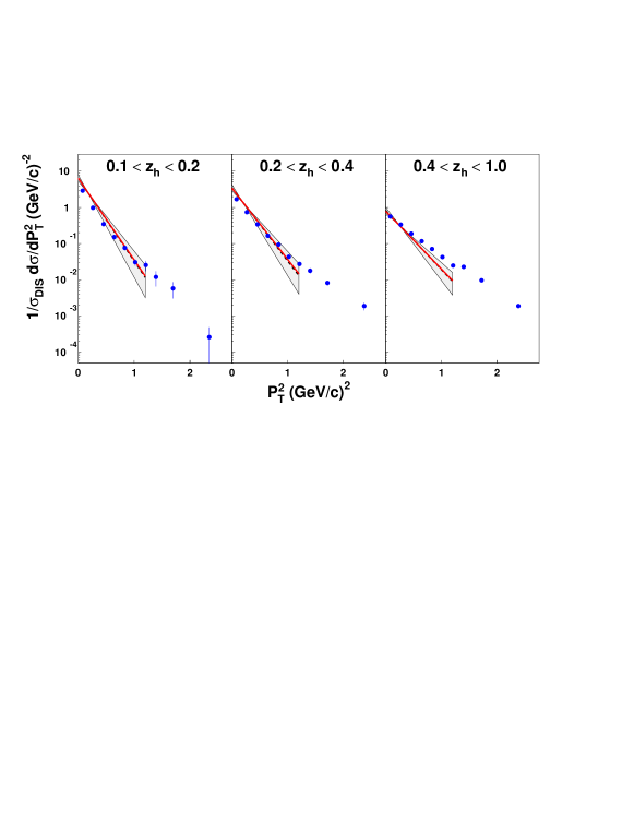
Figure 5: The normalized cross section $d\sigma/dP_{T}^{2}$: the dashed line is obtained with exact kinematics, while the solid bold line includes terms up to ${\cal O}({k_{\perp}}/{Q})$ only. The shadowed region corresponds to varying the parameters $\langle k_{\perp}^{2}\rangle$ and $\langle p_{\perp}^{2}\rangle$, given in Eq. (46) of the text, by 20%. The data are from Ref. EMCpt .

Other interesting EMC data EMCpt concern the $P_{T}^{2}$ dependence of the cross section for $\mu p$ and $\mu d$ scattering at incident beam energy between $100$ and $280$ GeV; also these data are strictly related to the values of $\langle k_{\perp}^{2}\rangle$ and $\langle p_{\perp}^{2}\rangle$. The quantity measured is given by

$$\frac{1}{\sigma_{DIS}}\,\frac{d\sigma}{dP_{T}^{2}}=\frac{1}{2\,\sigma_{DIS}}\,\int\!d\phi_{h}\,dx_{\!\scriptscriptstyle B}\,dQ^{2}\,dz_{h}\;\frac{d^{5}\sigma^{\ell p\to\ell hX}}{dx_{\!\scriptscriptstyle B}\,dQ^{2}\,dz_{h}\,d^{2}\mbox{\boldmath$P$}_{T}},$$ (41)

where $\sigma_{DIS}$ is the integrated DIS cross section from Eq. (10). In the integration of Eq. (41) the following experimental cuts have been imposed (see Ref. EMCpt for further details):

$$Q^{2}>5\;({\rm GeV}/c)^{2}\;,\;\;\;W^{2}<90\;{\rm GeV^{2}}\;,\;\;\;E_{h}>5\;{\rm GeV}$$

$$0.1<z_{h}<0.9\;,\;\;\;0.2<y<0.8\>.$$ (42)

Fig. 5 shows the comparison of our results with EMC data EMCpt for different ranges of $z_{h}$. The solid and dashed lines, which are here basically indistinguishable, are the results of our fits at first order and at all orders in $k_{\perp}/Q$ respectively. The shadowed region is spanned by varying the parameters $\langle k_{\perp}^{2}\rangle$ and $\langle p_{\perp}^{2}\rangle$ by $20$% and shows the sensitivity of our results on these parameters. The figure clearly show that, as expected, our LO approach is valid for $P_{T}$ values up to about $1$ GeV/$c$. At higher values NLO contributions from $\gamma^{*}q\to gq$ and $\gamma^{*}g\to q\bar{q}$ processes have to be taken into account.

Useful data on the $\phi_{h}$ and $P_{T}$ dependence were also found by the FNAL E665 collaboration E665 in $\mu p$ and $\mu d$ interactions at $490$ GeV. The quantity studied is

$$\langle\cos\phi_{h}\rangle=\frac{\int dx_{\!\scriptscriptstyle B}\,dQ^{2}\,dz_{h}\,d^{2}\mbox{\boldmath$P$}_{T}\,\cos\phi_{h}\,d^{5}\sigma}{\int dx_{\!\scriptscriptstyle B}\,dQ^{2}\,dz_{h}\,d^{2}\mbox{\boldmath$P$}_{T}\,d^{5}\sigma}$$ (43)

where $d^{5}\sigma$ denotes the fully differential cross section

$$d^{5}\sigma\equiv\frac{d^{5}\sigma^{\ell p\to\ell hX}}{dx_{\!\scriptscriptstyle B}\,dQ^{2}\,dz_{h}\,d^{2}\mbox{\boldmath$P$}_{T}}\>,$$ (44)

and where the integral over $P_{T}$ runs from $P_{T}^{cut}$ to $P_{T}^{max}\simeq 2.5$ GeV/$c$. According to the experimental setup E665 , the integration region in Eq. (43) is defined by:

$$Q^{2}>3\;({\rm GeV}/c)^{2}\;,\;\;\;300<W^{2}<900\;{\rm GeV^{2}}\;,$$

$$60<\nu<500\;{\rm GeV}\;,\;\;\;E_{h}>8\;{\rm GeV}\;,\;\;\;0.1<y<0.85\>.$$ (45)

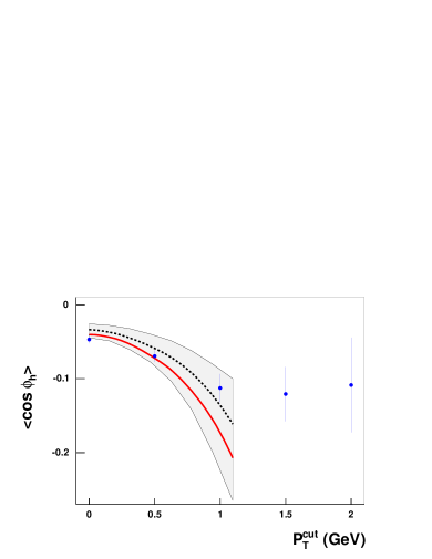
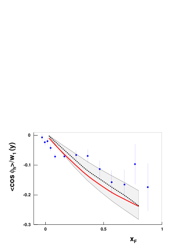
Figure 6: $\langle\cos\phi_{h}\rangle$, as given by Eq. (43), as a function of $P_{T}^{cut}$, left panel, and $x_{F}$, right panel: the dashed line is obtained with exact kinematics, while the solid bold line includes terms up to ${\cal O}({k_{\perp}}/{Q})$ only. The shadowed region corresponds to varying the parameters $\langle k_{\perp}^{2}\rangle$ and $\langle p_{\perp}^{2}\rangle$, given in Eq. (46) of the text, by 20%. $w_{1}(y)=\frac{(2-y)\sqrt{1-y}}{1+(1-y)^{2}}$. The data are from Ref. E665 , left panel, and Ref. EMC2 , right panel.

Fig. 6 shows the data E665 as a function of $P_{T}^{cut}$ compared with the results of our calculations; again, the solid bold line corresponds to the result we obtain by taking into account only $O(k_{\perp}/Q)$ terms, Eq. (38), whereas the dashed line corresponds to the exact kinematics, Eq. (31). We also show the EMC data on the $x_{F}$ dependence of $\langle\cos\phi_{h}\rangle/w_{1}(y)$ EMC2 ; they compare well with our results obtained by using Eq. (43) (in the right panel of Fig. 6 the theoretical curve corresponds to the calculation of $\langle\cos\phi_{h}\rangle/\langle w_{1}(y)\rangle$) with the experimental cuts of Ref. EMC2 and no integration over $z_{h}$ which is expressed in terms of $x_{F}$. The shadowed region is obtained by varying the parameters $\langle k_{\perp}^{2}\rangle$ and $\langle p_{\perp}^{2}\rangle$ by $20$%. Once more, Fig. 6 clearly shows that our calculation is valid for $P_{T}$ values up to about $1$ GeV/$c$, where NLO pQCD contributions ces ; nlo must be taken into account and our simple LO treatment can no longer be applied.

All sets of data described above depend crucially on the intrinsic motion in distribution and fragmentation functions; their combined analysis leads to the following best values of the parameters:

$$\langle k_{\perp}^{2}\rangle=0.25\;({\rm GeV}/c)^{2}\quad\quad\quad\langle p_{\perp}^{2}\rangle=0.20\;({\rm GeV}/c)^{2}\>.$$ (46)

One should notice that the above values have been derived from sets of data collected at different energy, $x_{\!\scriptscriptstyle B}$, $Q^{2}$ and $z_{h}$ ranges, looking at the combined production of all charged hadrons in SIDIS processes, and assuming constant values of $\langle k_{\perp}^{2}\rangle$ and $\langle p_{\perp}^{2}\rangle$, which allow analytical integration up to ${\cal O}(k_{\perp}/Q)$; these values are also assumed to be independent of the (light) quark flavor. A more refined analysis, introducing for example $x$ and $z$ dependences, would require the introduction of new unknown functions. At this stage, we stick to the constant best values (46) which, together with Eqs. (34) and (35), can only be considered as a consistent simple estimate and a convenient parametrization of the true intrinsic motion of quarks in nucleons and of hadrons in jets, supported by the available experimental information. In the next Section we adopt such a picture for the computation of pion and kaon SSA in SIDIS polarized processes, $\ell\,p^{\uparrow}\to\ell\,\pi\,X$ and $\ell\,p^{\uparrow}\to\ell\,K\,X$.

IV Sivers effect in polarized SIDIS

In this Section we consider the single spin asymmetry $A_{UT}$ measured in $ep^{\uparrow}\to e\pi X$ processes by the HERMES collaboration at DESY, using a transversely polarized proton target hermUT . Our aim is that of obtaining information on the quark Sivers functions, which can be isolated and directly accessed by studying the weighted transverse spin asymmetry $A_{UT}^{\sin(\phi_{\pi}-\phi_{S})}$ bm . These functions are then compared with those obtained from the study of SSA in $p^{\uparrow}p$ processes. They are also used to estimate the contribution of the Sivers mechanism alone to the weighted SSA $A_{UL}^{\sin\phi_{\pi}}$, measured by the HERMES collaboration in the lepton scattering off a longitudinally polarized proton target hermUL . Moreover, expectations for $A_{UT}^{\sin(\phi_{\pi}-\phi_{S})}$ in the COMPASS kinematical regions are computed and compared with preliminary COMPASS data compUT and predictions for kaon asymmetries $A_{UT}^{\sin(\phi_{K}-\phi_{S})}$ at HERMES are given.

Let us recall the origin of the SSA in SIDIS, as originated by the Sivers mechanism siv . The unpolarized quark (and gluon) distributions inside a transversely polarized proton (generically denoted by $p^{\uparrow}$, with $p^{\downarrow}$ denoting the opposite polarization state) can be written as:

$$f_{q/p^{\uparrow}}(x,\mbox{\boldmath$k$}_{\perp})=f_{q/p}(x,k_{\perp})+\frac{1}{2}\,\Delta^{N}f_{q/p^{\uparrow}}(x,k_{\perp})\;{{\mbox{\boldmath$S$}}_{{}_{T}}}\cdot(\hat{\mbox{\boldmath$P$}}\times\hat{\mbox{\boldmath$k$}}_{\perp})\;,$$ (47)

where $P$ and ${\mbox{\boldmath$S$}}_{{}_{T}}$ are respectively the proton momentum and transverse polarization vector, and $\mbox{\boldmath$k$}_{\perp}$ is the parton transverse momentum; transverse refers to the proton direction. Eq. (47) implies

$$f_{q/p^{\uparrow}}(x,\mbox{\boldmath$k$}_{\perp})+f_{q/p^{\downarrow}}(x,\mbox{\boldmath$k$}_{\perp})=2f_{q/p}(x,k_{\perp})\;,$$

$$f_{q/p^{\uparrow}}(x,\mbox{\boldmath$k$}_{\perp})-f_{q/p^{\downarrow}}(x,\mbox{\boldmath$k$}_{\perp})=\Delta^{N}f_{q/p^{\uparrow}}(x,k_{\perp})\;{{\mbox{\boldmath$S$}}_{{}_{T}}}\cdot(\hat{\mbox{\boldmath$P$}}\times\hat{\mbox{\boldmath$k$}}_{\perp})\;,$$ (48)

where $f_{q/p}(x,k_{\perp})$ is the unpolarized parton density and $\Delta^{N}f_{q/p^{\uparrow}}(x,k_{\perp})$ is referred to as the Sivers function. Notice that, as requested by parity invariance, the scalar quantity ${\mbox{\boldmath$S$}}_{{}_{T}}\cdot(\hat{\mbox{\boldmath$P$}}\times\hat{\mbox{\boldmath$k$}}_{\perp})$ singles out the polarization component perpendicular to the $\mbox{\boldmath$P$}-\mbox{\boldmath$k$}_{\perp}$ plane. For a proton moving along $-z$ and a generic transverse polarization vector ${\mbox{\boldmath$S$}}_{{}_{T}}=|{\mbox{\boldmath$S$}}_{{}_{T}}|\,(\cos\phi_{S},\sin\phi_{S},0)$ (see Fig. 3) one has:

$${\mbox{\boldmath$S$}}_{{}_{T}}\cdot(\hat{\mbox{\boldmath$P$}}\times\hat{\mbox{\boldmath$k$}}_{\perp})=|{\mbox{\boldmath$S$}}_{{}_{T}}|\,\sin(\varphi-\phi_{S})\equiv|{\mbox{\boldmath$S$}}_{{}_{T}}|\,\sin\phi_{Siv}\,,$$ (49)

where $(\varphi-\phi_{S})=\phi_{Siv}$ is the Sivers angle.

The cross section for the scattering of an unpolarized lepton off a polarized proton, in the configuration of Fig. 3, can then simply be written as, see Eq. (31),

$$d^{6}\sigma^{\uparrow}=\frac{1}{2\pi}\sum_{q}\int{d^{2}\mbox{\boldmath$k$}_{\perp}}\;f_{q/p^{\uparrow}}(x,k_{\perp})\;\frac{d\hat{\sigma}^{\ell q\to\ell q}}{dQ^{2}}\;J\;\frac{z}{z_{h}}\;D_{q}^{h}(z,p_{\perp})$$ (50)

where $d^{6}\sigma^{\uparrow}$ stands for

$$d^{6}\sigma^{\uparrow}\equiv\frac{d^{6}\sigma^{\ell p^{\uparrow}\to\ell hX}}{dx_{\!\scriptscriptstyle B}\,dQ^{2}\,dz_{h}\,d^{2}\mbox{\boldmath$P$}_{T}\,d\phi_{S}}\>,$$ (51)

and where the $\phi_{S}$ dependence is contained in $f_{q/p^{\uparrow}}(x,\mbox{\boldmath$k$}_{\perp})$. The $\phi_{S}$ dependence originates from the fact that, with transversely polarized protons, the cross section depends also on the angle between the polarization vector and the leptonic plane; in the configuration of Fig. 3 this is simply $\phi_{S}-\phi_{\ell^{\prime}}$ = $\phi_{S}$, having chosen $\phi_{\ell^{\prime}}$ to be zero, with $\phi_{S}$ varying event by event. In actual experiments variables are measured in a different frame (for example the laboratory frame where the lepton moves along the $z$-axis and the proton is at rest); a comprehensive set of relations between the different frames can be found in Ref. aram . Let us only notice here that the difference between the azimuthal angles of the final lepton in the frame of Fig. 3 and in the laboratory frame is of the ${\cal O}(k_{\perp}^{2}/Q^{2})$.

This leads to the possibility of a non vanishing transverse single spin asymmetry, the analyzing power

$$A=\frac{d^{6}\sigma^{\uparrow}-d^{6}\sigma^{\downarrow}}{d^{6}\sigma^{\uparrow}+d^{6}\sigma^{\downarrow}}\>,$$ (52)

which is given, according to Eqs. (50) and (48) by:

$$A=\frac{\displaystyle\sum_{q}\int{d^{2}\mbox{\boldmath$k$}_{\perp}}\;\Delta^{N}f_{q/p^{\uparrow}}(x,k_{\perp})\;[{\mbox{\boldmath$S$}}_{{}_{T}}\cdot(\hat{\mbox{\boldmath$P$}}\times\hat{\mbox{\boldmath$k$}}_{\perp})]\,\frac{d\hat{\sigma}^{\ell q\to\ell q}}{dQ^{2}}\;J\;\frac{z}{z_{h}}\;D_{q}^{h}(z,p_{\perp})}{\displaystyle 2\sum_{q}\int{d^{2}\mbox{\boldmath$k$}_{\perp}}\;f_{q}(x,k_{\perp})\;\frac{d\hat{\sigma}^{\ell q\to\ell q}}{dQ^{2}}\;J\;\frac{z}{z_{h}}\;D_{q}^{h}(z,p_{\perp})}\>\cdot$$ (53)

The above equation gives the transverse SSA originated by the Sivers mechanism alone, properly taking into account all intrinsic motions. As it is written it depends on $x_{\!\scriptscriptstyle B},Q^{2},z_{h},\mbox{\boldmath$p$}_{{}_{T}}$ and $\phi_{S}$: of course, in order to increase statistics and according to the experimental setups, both the numerator and denominator of Eq. (53) can be integrated over some of the variables.

HERMES first data hermUL were gathered in the scattering of unpolarized leptons ($U$) off “longitudinally” ($L$) polarized proton, where “longitudinal” means antiparallel to the lepton direction in the proton rest frame. Such a direction has a small transverse component, in the $\gamma^{*}p$ frame, with respect to the proton direction, that is

$${\mbox{\boldmath$S$}}_{{}_{T}}=-\sin\theta_{\gamma}\,(1,0,0)\quad\>{\mbox{\boldmath$S$}}_{{}_{T}}\cdot(\hat{\mbox{\boldmath$P$}}\times\hat{\mbox{\boldmath$k$}}_{\perp})=-\sin\theta_{\gamma}\,\sin\varphi\quad\>\sin\theta_{\gamma}\simeq\frac{2\,m_{p}\,x_{\!\scriptscriptstyle B}}{Q}\,\sqrt{1-y}\>.$$ (54)

HERMES data are presented for the $\sin\phi_{h}$ moment of the analyzing power,

$$A^{\sin\phi_{h}}=2\,\frac{\int d\phi_{h}\,[d\sigma^{\uparrow}-d\sigma^{\downarrow}]\,\sin\phi_{h}}{\int d\phi_{h}\,[d\sigma^{\uparrow}+d\sigma^{\downarrow}]}\>,$$ (55)

which, from Eq. (53), is

$$A^{\sin\phi_{h}}_{UL}=\frac{\displaystyle-\sum_{q}\int{d\phi_{h}\,d^{2}\mbox{\boldmath$k$}_{\perp}}\;\Delta^{N}f_{q/p^{\uparrow}}(x,k_{\perp})\sin\theta_{\gamma}\sin\varphi\;\frac{d\hat{\sigma}^{\ell q\to\ell q}}{dQ^{2}}\;J\;\frac{z}{z_{h}}\;D_{q}^{h}(z,p_{\perp})\sin\phi_{h}}{\displaystyle\sum_{q}\int{d\phi_{h}\,d^{2}\mbox{\boldmath$k$}_{\perp}}\;f_{q}(x,k_{\perp})\;\frac{d\hat{\sigma}^{\ell q\to\ell q}}{dQ^{2}}\;J\;\frac{z}{z_{h}}\;D_{q}^{h}(z,p_{\perp})}$$ (56)

where both numerator and denominator can be integrated over some of the variables. Eq. (56) gives the contribution of the Sivers function to $A^{\sin\phi_{h}}_{UL}$. Notice that it is kinematically suppressed by the $\sin\theta_{\gamma}$ value, Eq. (54), and that other contributions might be equally important; they can originate from the Collins mechanism or from higher-twist terms.

More recently, data were obtained with a transversely polarized ($T$) proton target hermUT , ${\mbox{\boldmath$S$}}_{{}_{T}}\cdot(\hat{\mbox{\boldmath$P$}}\times\hat{\mbox{\boldmath$k$}}_{\perp})=\sin(\varphi-\phi_{S})$, and presented for the $\sin(\phi_{h}-\phi_{S})$ moment of the analyzing power, which singles out the Sivers contribution bm . Eq. (53) in this case gives

$$\!\!\!\!A^{\sin(\phi_{h}-\phi_{S})}_{UT}=$$ (57)

$$\hskip-18.0pt\frac{\displaystyle\sum_{q}\int{d\phi_{S}\,d\phi_{h}\,d^{2}\mbox{\boldmath$k$}_{\perp}}\;\Delta^{N}f_{q/p^{\uparrow}}(x,k_{\perp})\sin(\varphi-\phi_{S})\;\frac{d\hat{\sigma}^{\ell q\to\ell q}}{dQ^{2}}\;J\;\frac{z}{z_{h}}\;D_{q}^{h}(z,p_{\perp})\sin(\phi_{h}-\phi_{S})}{\displaystyle\sum_{q}\int{d\phi_{S}\,d\phi_{h}\,d^{2}\mbox{\boldmath$k$}_{\perp}}\;f_{q}(x,k_{\perp})\;\frac{d\hat{\sigma}^{\ell q\to\ell q}}{dQ^{2}}\;J\;\frac{z}{z_{h}}\;D_{q}^{h}(z,p_{\perp})}\>\cdot$$

We use Eq. (57) to compute $A^{\sin(\phi_{h}-\phi_{S})}_{UT}$, which can only receive contributions from the Sivers mechanism, and compare it with data, in order to gather information on the Sivers function $\Delta^{N}f_{q/p^{\uparrow}}(x,k_{\perp})$.

IV.1 Parameterization of the Sivers function

We parameterize, for each light quark flavour $q=u,d$, the Sivers function in the following factorized form col ; noiD :

$$\Delta^{N}f_{q/p^{\uparrow}}(x,k_{\perp})=2\,{\cal N}_{q}(x)\,h(k_{\perp})\,f_{q/p}(x,k_{\perp})\;,$$ (58)

where

$${\cal N}_{q}(x)=N_{q}\,x^{a_{q}}(1-x)^{b_{q}}\,\frac{(a_{q}+b_{q})^{(a_{q}+b_{q})}}{a_{q}^{a_{q}}b_{q}^{b_{q}}}\;,$$ (59)

$$h(k_{\perp})=\frac{2k_{\perp}\,M}{k_{\perp}^{2}+M^{2}}\;,$$ (60)

where $N_{q}$, $a_{q}$, $b_{q}$ and $M$ (GeV/$c$) are parameters. $f_{q/p}(x,k_{\perp})$ is the unpolarized distribution function defined in Eq. (34). Since $h(k_{\perp})\leq 1$ and since we allow the constant parameter $N_{q}$ to vary only inside the range $[-1,1]$ so that $|{\cal N}_{q}(x)|\leq 1$ for any $x$, the positivity bound for the Sivers function is automatically fulfilled:

$$\frac{|\Delta^{N}f_{q/p^{\uparrow}}(x,k_{\perp})|}{2f_{q/p}(x,k_{\perp})}\leq 1\;.$$ (61)

As an alternative parameterization for $h(k_{\perp})$ we have also used

$$h^{\prime}(k_{\perp})=\sqrt{2e}\,\frac{k_{\perp}}{M^{\prime}}\,e^{-k_{\perp}^{2}/M^{\prime 2}}.$$ (62)

The two parameterizations (60) and (62) are indeed equivalent at low $k_{\perp}$, but they differ at large values of $k_{\perp}$. Nevertheless, we have checked that, once multiplied by the Gaussian function of $k_{\perp}$ contained in the definition of $f(x,k_{\perp})$ [see Eq. (34)], they give basically the same $k_{\perp}$ dependence to the Sivers function over the whole range, as shown in Fig. 7 ($M^{2}=0.25$ (GeV/$c$)² and $M^{\prime 2}=0.36$ (GeV/$c$)²).

Figure 7: The product $h(k_{\perp})\cdot g(k_{\perp})$, solid line, compared with the product $h^{\prime}(k_{\perp})\cdot g(k_{\perp})$, dashed line, as a function of $k_{\perp}$.

The parameterization of Eq. (62) allows to easily perform, at ${\cal O}(k_{\perp}/Q)$, an analytical integration of Eq. (57), leading to an explicit approximate expression for the single spin asymmetry:

$$A_{UT}^{\sin(\phi_{h}-\phi_{S})}(x_{\!\scriptscriptstyle B},z_{h},P_{T})\simeq\frac{\Delta\sigma_{Siv}}{\sigma_{0}}\;,$$ (63)

where

$$\displaystyle\Delta\sigma_{Siv}(x_{\!\scriptscriptstyle B},y,z_{h},P_{T})=\frac{2\pi\alpha^{2}}{x_{\!\scriptscriptstyle B}\,y^{2}s}\,\left(1+(1-y)^{2}\right)\sum_{q}e_{q}^{2}\,2{\cal N}_{q}(x_{\!\scriptscriptstyle B})\,f_{q}(x_{\!\scriptscriptstyle B})\,D_{q}^{h}(z_{h})$$

$$\displaystyle z_{h}P_{T}\frac{\sqrt{2e}\widehat{\langle k_{\perp}^{2}\rangle}^{2}}{M^{\prime}\widehat{\langle P_{T}^{2}\rangle}^{2}\langle k_{\perp}^{2}\rangle}\exp{\left(-\frac{P_{T}^{2}}{\widehat{\langle P_{T}^{2}\rangle}}\right)},$$ (64)

and

$$\displaystyle\sigma_{0}(x_{\!\scriptscriptstyle B},y,z_{h},P_{T})=2\pi\frac{2\pi\alpha^{2}}{x_{\!\scriptscriptstyle B}\,y^{2}s}\,\left(1+(1-y)^{2}\right)\sum_{q}e_{q}^{2}\,f_{q}(x_{\!\scriptscriptstyle B})\,D_{q}^{h}(z_{h})$$

$$\displaystyle\frac{1}{\pi\langle P_{T}^{2}\rangle}\exp{\left(-\frac{P_{T}^{2}}{\langle P_{T}^{2}\rangle}\right)},$$ (65)

where

$$\widehat{\langle k_{\perp}^{2}\rangle}=\frac{M^{\prime 2}\,\langle k_{\perp}^{2}\rangle}{M^{\prime 2}+\langle k_{\perp}^{2}\rangle},\quad\widehat{\langle P_{T}^{2}\rangle}=\langle p_{\perp}^{2}\rangle+z_{h}^{2}\,\widehat{\langle k_{\perp}^{2}\rangle}\,,$$ (66)

and $\langle P_{T}^{2}\rangle$ is given in Eq. (39). Eq. (64) shows that $A_{UT}^{\sin(\phi_{h}-\phi_{S})}=0$ when $z_{h}=0$ or $P_{T}=0$.

IV.2 HERMES data and Sivers functions

Let us now try to understand the HERMES data on $A^{\sin(\phi_{\pi}-\phi_{S})}_{UT}$ hermUT , according to Eq. (57) (exact kinematics) or Eqs. (63)–(66) (kinematics up to ${\cal O}(k_{\perp}/Q)$). As in Section III, the unpolarized distribution functions are taken from Ref. MRST01 and the fragmentation functions from Ref. Kretzer . In the numerator we take into account only the Sivers contribution of $u$ and $d$ quarks and antiquarks, with separate valence and sea functions. More precisely, we adopt the following form for the Sivers functions:

$$\Delta^{N}f_{q/p^{\uparrow}}(x,k_{\perp})=2\,{\cal N}_{q}(x)\,h^{\prime}(k_{\perp})\,f_{q/p}(x,k_{\perp})\;,$$ (67)

where ${\cal N}_{q}$ is given in Eq. (59), $h^{\prime}$ in Eq. (62) and $q=u_{v},d_{v},u_{s},d_{s},\bar{u},\bar{d}$. For the sea quark contributions we assume:

$$\Delta^{N}f_{q_{s}/p^{\uparrow}}(x,k_{\perp})=\Delta^{N}f_{\bar{q}/p^{\uparrow}}(x,k_{\perp})\;,$$ (68)

for a total of 4 unknown functions, each depending on 3 parameters; in addition, $h^{\prime}(k_{\perp})$ depends on the parameter $M^{\prime}$.

We fit the HERMES data on $A^{\sin(\phi_{\pi}-\phi_{S})}_{UT}$ exploiting the simplified expressions (63)–(66). The resulting best values for the 13 free parameters are shown in Table 1.

$N_{u_{v}}$ =	$0.42\pm 0.18$	$N_{d_{v}}$ =	$-1.0\pm 1.8$
$a_{u_{v}}$ =	$0.0\pm 3.3$	$a_{d_{v}}$ =	$1.1\pm 1.2$
$b_{u_{v}}$ =	$2.6\pm 1.8$	$b_{d_{v}}$ =	$5.0\pm 3.6$
$N_{\bar{u}}$ =	$1.0\pm 1.9$	$N_{\bar{d}}$ =	$-1.0\pm 1.9$
$a_{\bar{u}}$ =	$0.52\pm 0.43$	$a_{\bar{d}}$ =	$0.0\pm 4.5$
$b_{\bar{u}}$ =	$0.0\pm 3.1$	$b_{\bar{d}}$ =	$0.0\pm 2.8$
$M^{\prime 2}$ =	$0.36\pm 0.43\;{\rm(GeV}/c)^{2}$	$\chi^{2}/{d.o.f.}$ =	$0.89$

Table 1: Best values of the parameters of the Sivers functions.

The errors are generated by the MINUIT minimizer. The large errors reflect the large errors of the data and the scarce available information.

Our fit is shown in Fig. 8. The solid bold line takes into account terms up to ${\cal O}(k_{\perp}/Q)$, the dashed line is obtained with the full exact $\mbox{\boldmath$k$}_{\perp}$ kinematics, Eq. (57). In both cases the parameters of Table 1 are used. The shadowed region corresponds to one-sigma deviation at 90% CL and was calculated using the errors (Table 1) and the parameter correlation matrix generated by MINUIT, minimizing and maximizing the function under consideration, in a 13-dimensional parameter space hyper-volume corresponding to one-sigma deviation. Notice that, as expected, the results obtained with exact or approximate kinematics are very similar.

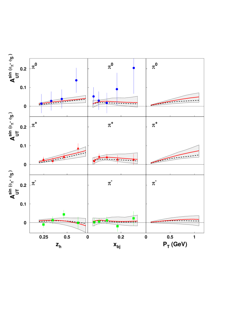
Figure 8: HERMES data on $A_{UT}^{\sin(\phi_{\pi}-\phi_{S})}$ hermUT for scattering off a transversely polarized proton target and pion production. The curves are the results of our fits, with exact kinematics (dashed line) or keeping only terms up to ${\cal O}({k_{\perp}}/{Q})$ (solid bold line). The shadowed region corresponds to the theoretical uncertainty due to the parameter errors. Data on the $P_{T}$ dependence of $A_{UT}^{\sin(\phi_{\pi}-\phi_{S})}$ are not available yet, and the third column of the figure gives our predictions.

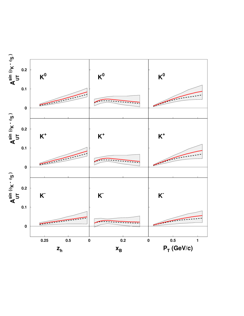
Figure 9: Predictions for kaon asymmetries $A_{UT}^{\sin(\phi_{h}-\phi_{S})}$ at HERMES kinematics for scattering off a transversely polarized proton target. The curves correspond to calculation with exact kinematics (dashed line) or keeping only terms up to ${\cal O}({k_{\perp}}/{Q})$ (solid bold line). The shadowed region corresponds to the theoretical uncertainty due to the parameter errors.

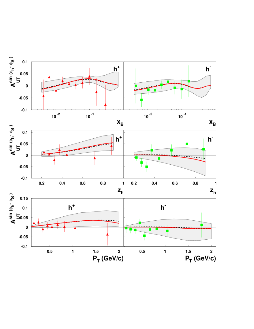
Figure 10: COMPASS preliminary data compUT on $A_{UT}^{\sin(\phi_{h}-\phi_{S})}$ for scattering off a transversely polarized deuteron target and the production of positively ($h^{+}$) and negatively ($h^{-}$) charged hadrons. The curves show our predictions, according to the values of the parameters for the Sivers functions given in Table 1 and obtained from fitting the HERMES data on $A_{UT}^{\sin(\phi_{\pi}-\phi_{S})}$. Again, the dashed line refers to exact kinematics, Eq. (57), while the solid bold line is obtained by keeping only terms up to ${\cal O}({k_{\perp}}/{Q})$. The shadowed region shows the theoretical uncertainty due to the parameter errors.

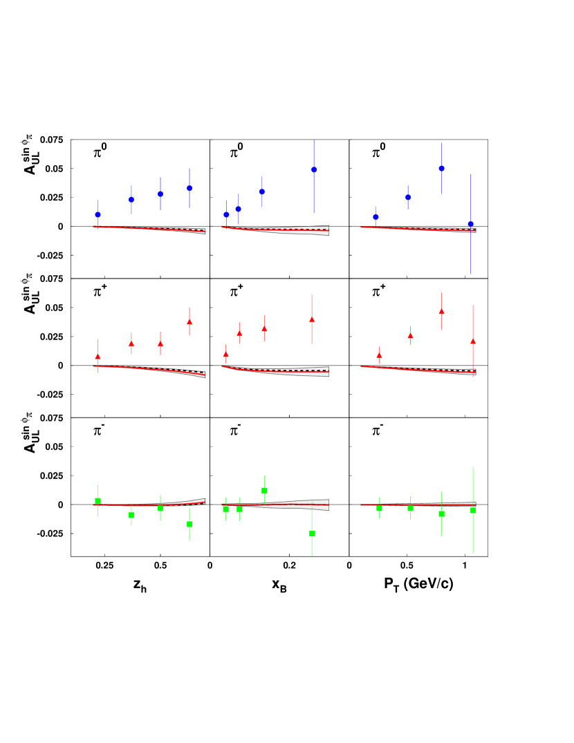
Figure 11: HERMES data on $A_{UL}^{\sin\phi_{\pi}}$ hermUL for scattering off a longitudinally polarized proton target and pion production. The curves show the contribution of our Sivers functions alone, with exact kinematics (Eq. (56), dashed line) or keeping only terms up to ${\cal O}({k_{\perp}}/{Q})$ (solid bold line). The shadowed region corresponds to the theoretical uncertainty due to the parameter errors.

We show the weighted SSA $A_{UT}^{\sin(\phi_{\pi}-\phi_{S})}$ as a function of one variable at a time, either $z_{h}$ or $x_{\!\scriptscriptstyle B}$ or $P_{T}$; the integration over the other variables has been performed consistently with the cuts of the HERMES experiment, at $p_{lab}=27.57$ GeV/$c$:

$$Q^{2}>1\;({\rm GeV}/c)^{2}\quad W^{2}>10\;{\rm GeV}^{2}\quad P_{T}>0.05\;{\rm GeV}/c$$

$$0.023<x_{\!\scriptscriptstyle B}<0.4\quad\quad 0.2<z_{h}<0.7\quad\quad 0.1<y<0.85\>$$ (69)

$$2<E_{h}<15\>{\rm GeV}.$$

A few comments are necessary for the interpretation of the results.

• Fig. 8 shows that a good agreement with experiments can be obtained. However, due to the present quality of this first set of data, the extracted Sivers functions are not well constrained and large uncertainties are still possible.

• We notice that we have checked the compatibility of the HERMES data on $A_{UT}^{\sin(\phi_{\pi}-\phi_{S})}$ with the assumption of no Sivers effect, $\Delta^{N}f\equiv 0$. The data show that the probability of a zero value for the Sivers function is less than $0.1$%.

• It is interesting to compare the Sivers functions obtained here, Eqs. (67), (59), (62) and Table 1, with those obtained by fitting the SSA observed by the E704 Collaboration in $p^{\uparrow}\,p\to\pi\,X$ processes fu . As stressed in the Introduction the question regarding the universality of the Sivers functions is a debated and open one. The comparison of our results with Eqs. (46)-(48) of Ref. fu is not straightforward: one should keep in mind that there is no sea contribution in Ref. fu and that the HERMES data are sensitive to much smaller $x$ values than the E704 ones (which strongly depend on large $x$ values). Moreover, the average $k_{\perp}$ and $p_{\perp}$ values adopted in Ref. fu are somewhat higher than those adopted here, derived with simplifying assumptions from data on azimuthal dependences in SIDIS processes. Despite all this, there is a clear indication that the two sets of Sivers functions are not incompatible. The functions of Ref. fu , if used in our Eq. (57) or (63)–(66), still allow a reasonable description of the HERMES data. On the other hand, our Sivers functions of Table 1, if used to describe the SSA observed by E704 experiment e704 , would overestimate the data at small $x_{F}$ values; this could be easily corrected by gluon contributions (gluon Sivers function) not considered in Ref. fu and absent at LO in SIDIS.

  We do not wish, at this stage and with the limited amount of available experimental information, to further stress such a point; the issue of the uniqueness of the Sivers functions in SIDIS and $p\,p\to\pi\,X$ processes is still far from being phenomenologically established. We simply conclude that it cannot be excluded by existing data.

• The Sivers functions obtained here are compatible with those extracted very recently from an analysis of $P_{T}$ weighted HERMES data performed in Ref. sivers_efremov .

Leaving aside the question of the dependence of the Sivers functions on the different physical processes, the consistency of our results can be checked within SIDIS processes, by using our functions to give predictions for other measured SSA. This can be done by computing, with our sets of Sivers functions, the values of $A_{UT}^{\sin(\phi_{\pi}-\phi_{S})}$ expected by the COMPASS experiment at CERN, which collects data in $\mu d\to\mu h^{\pm}X$ processes at $p_{lab}=$ 160 GeV/$c$, spanning a different kinematical region. Some preliminary results are already available compUT . We neglect nuclear corrections and use the isospin symmetry in order to obtain the parton distribution functions of the deuterium. According to COMPASS experimental setup, we use the following cuts in the numerator and denominator integration of Eq. (57):

$$Q^{2}>1\;({\rm GeV}/c)^{2}\quad W^{2}>25\;{\rm GeV}^{2}\quad P_{T}>0.1\;{\rm GeV}/c$$

$$E_{h}>4\;{\rm GeV}\quad\quad 0.2<z_{h}<0.9\quad\quad 0.1<y<0.9\>.$$ (70)

The predictions of our model are presented in Fig. 10 and compared with the available preliminary data compUT . Within the large errors, we find a good agreement, showing the consistency of the model.

We have also computed $A_{UT}^{\sin(\phi_{K}-\phi_{S})}$ for kaon production, $h=K$, which could be measured by HERMES; we have imposed the kinematical cuts of Eq. (69), using the fragmentation functions given in Ref. Kretzer . Our results are given in Fig. 9.

Finally, we have considered the HERMES data on $A_{UL}^{\sin\phi_{\pi}}$ obtained in the semi-inclusive electro-production of pions on a longitudinally polarized hydrogen target hermUL . We have computed the Sivers contribution to this quantity, according to Eq. (56), again with our set of Sivers functions, and compared with data. Notice that no agreement should be necessarily expected, as $A_{UL}^{\sin\phi_{\pi}}$ can be originated also (even dominantly) from the Collins mechanisms or higher-twist terms. Using the following experimental cuts:

$$\hskip-18.0pt1<Q^{2}<15\;({\rm GeV}/c)^{2}\quad W^{2}>4\;{\rm GeV^{2}}\quad P_{T}>0.05\;{\rm GeV}/c\quad 4.5<E_{h}<13.5\;{\rm GeV}$$

$$\hskip-18.0pt0.023<x_{\!\scriptscriptstyle B}<0.4\quad\quad 0.2<z_{h}<0.7\quad\quad 0.2<y<0.85\>,$$ (71)

we obtain the results depicted in Fig. 11.

One can conclude that our Sivers functions extracted from the HERMES data on $A_{UT}^{\sin(\phi_{\pi}-\phi_{S})}$ only give a negligible contribution to $A_{UL}^{\sin\phi_{\pi}}$. Not only, but the Sivers mechanism contributes with opposite signs to the transverse and longitudinal SSA, as can be seen from Eqs. (56) and (57). This implies that Collins mechanism and/or higher-twist contributions are likely to be wholly responsible for the observed $A_{UL}^{\sin\phi_{\pi}}$, as suggested by some authors c-s1 .

V Comments and conclusions

We have studied inclusive and semi-inclusive DIS processes at leading order in the QCD parton model, in the $\gamma^{*}p$ c.m. frame and in the small $P_{T}\simeq\Lambda_{\rm QCD}\simeq k_{\perp}$ region, where intrinsic momenta dominate the final hadron azimuthal and $P_{T}$ distributions. We have adopted a factorized parton model scheme and exactly taken into account all intrinsic motions, of quarks inside the proton ($\mbox{\boldmath$k$}_{\perp}$) and of the final hadron with respect to the fragmenting quark ($\mbox{\boldmath$p$}_{\perp}$).

We have attempted a consistent treatment, assuming simple Gaussian $k_{\perp}$ and $p_{\perp}$ distributions and extracting from various sets of SIDIS data estimates about the average values $\langle k_{\perp}\rangle$ and $\langle p_{\perp}\rangle$. Such values are assumed to be constant, respectively in $x$ and $z$, and to be energy independent. Simple parameterizations for the quark Sivers functions have been introduced.

The resulting picture has been applied to the computation of the weighted SSA $A_{UT}^{\sin(\phi_{\pi}-\phi_{S})}$, at LO in QCD parton model, which directly depends on the intrinsic motions and the Sivers functions. The HERMES data clearly show a non zero Sivers effect; by a comparison with these data some rough estimates of the Sivers functions for $u$ and $d$ (both valence and sea) quarks have been obtained. These functions not only describe well the HERMES data, but are also in agreement with some COMPASS preliminary data on $A_{UT}^{\sin(\phi_{\pi}-\phi_{S})}$, which refer to different kinematical regions. The same functions are found to give negligible contributions, with the wrong sign, to the measured longitudinal SSA $A_{UL}^{\sin\phi_{\pi}}$. This asymmetry can indeed be originated by the Collins mechanism and higher-twist contributions. Predictions for $A_{UT}^{\sin(\phi_{K}-\phi_{S})}$ for kaon production at HERMES have been given.

The quark Sivers functions extracted from the HERMES data on pion $A_{UT}^{\sin(\phi_{\pi}-\phi_{S})}$ have been compared with the Sivers functions obtained by fitting the E704 data on SSA in $p^{\uparrow}\,p\to\pi\,X$ processes. Such a comparison cannot be considered as conclusive, as it refers to situations with different kinematical regions and different assumptions about the sea contribution; however, it does not exclude the possibility that the two sets of Sivers functions – those active in SIDIS and in $p\,p$ processes – are the same. In particular the signs seem to be the same in the two cases. Theoretical arguments support an opposite sign for the Sivers functions in SIDIS and Drell-Yan processes, with no conclusions concerning $p\,p$ interactions. Our Sivers functions are compatible with those obtained in Ref. sivers_efremov .

A phenomenological study of SSA and azimuthal dependences, within a factorization scheme with unintegrated parton distribution and fragmentation functions, is now possible. SIDIS processes with measurements of the Cahn effect, and the various SSA $A_{UL}^{\sin\phi_{h}}$, $A_{UT}^{\sin(\phi_{h}-\phi_{S})}$ and $A_{UT}^{\sin(\phi_{h}+\phi_{S})}$ provide a rich ground to be further explored, both theoretically and experimentally.

Appendix A

It is known from symmetry principles that, within the one photon exchange approximation, the double inclusive cross section for unpolarized SIDIS processes, $\ell\,p\to\ell\,h\,X$, can have a dependence on the azimuthal angle $\phi_{h}$ of the final hadron (in the reference frame of Fig. 3) of the form aram

$$\frac{d^{5}\sigma^{\ell p\to\ell hX}}{dx_{\!\scriptscriptstyle B}\,dQ^{2}\,dz_{h}\,d^{2}\mbox{\boldmath$P$}_{T}}=A+B\cos\phi_{h}+C\cos 2\phi_{h}$$ (72)

where $A,B$ and $C$ are scalar quantities which do not depend on $\phi_{h}$. This is explicitly visible in the approximate expression (38) and we wonder whether Eq. (31) satisfies in general such a condition.

From Eqs. (4), (34), (35), (26) and (28) one can see that Eq. (31) is of the form

$$\int d^{2}\mbox{\boldmath$k$}_{\perp}\left[a+b\,\mbox{\boldmath$\ell$}\cdot\mbox{\boldmath$k$}_{\perp}+c\,(\mbox{\boldmath$\ell$}\cdot\mbox{\boldmath$k$}_{\perp})^{2}\right]\,F(\mbox{\boldmath$P$}_{T}\cdot\mbox{\boldmath$k$}_{\perp},\dots)$$ (73)

where $a,b$ and $c$ do not depend on angles and the $\dots$ stands for scalar variables which also do not depend on azimuthal angles.

As a consequence, a tensorial analysis of Eq. (73) shows that Eq. (31) can only contain azimuthal dependences through the integrals:

$$b\>\mbox{\boldmath$\ell$}\cdot\int d^{2}\mbox{\boldmath$k$}_{\perp}\,\mbox{\boldmath$k$}_{\perp}F(\mbox{\boldmath$P$}_{T}\cdot\mbox{\boldmath$k$}_{\perp})\sim\mbox{\boldmath$\ell$}\cdot\mbox{\boldmath$P$}_{T}\sim\cos\phi_{h}$$

$$c\>\ell_{i}\,\ell_{j}\int d^{2}\mbox{\boldmath$k$}_{\perp}\>(k_{\perp})_{i}\,(k_{\perp})_{j}\,F(\mbox{\boldmath$P$}_{T}\cdot\mbox{\boldmath$k$}_{\perp})\sim\ell_{i}\,\ell_{j}\,(P_{T})_{i}\,(P_{T})_{j}\sim\cos^{2}\phi_{h}=\frac{1+\cos 2\phi_{h}}{2}$$

which agree with Eq. (72).

References

• (1) For a very recent paper on the QCD evolution of unintegrated parton distributions and a comprehensive list of all relevant previous references, see E.R. Arriola and W. Broniowski, Phys. Rev. D70 (2004) 034012
• (2) R.D. Field and R.P. Feynman, Phys. Rev. D15 (1977) 2590; R.P. Feynman, R.D. Field and G.C. Fox, Phys. Rev. D18 (1978) 3320
• (3) R.N. Cahn, Phys. Lett. B78 (1978) 269; Phys. Rev. D40 (1989) 3107
• (4) A. Konig and P. Kroll, Z. Phys. C16 (1982) 89
• (5) EMC Collaboration, J.J. Aubert et al., Phys. Lett. B130 (1983) 118
• (6) EMC Collaboration, M. Arneodo et al., Z. Phys. C34 (1987) 277
• (7) U. D’Alesio and F. Murgia, Phys. Rev. D70 (2004) 074009
• (8) For a recent review paper see V. Barone, A. Drago and P. Ratcliffe, Phys. Rept. 359 (2002) 1
• (9) HERMES Collaboration, A. Airapetian et al., Phys. Rev. Lett. 84 (2000) 4047; Phys. Rev. D64 (2001) 097101
• (10) HERMES Collaboration, A. Airapetian et al., Phys. Rev. Lett. 94 (2005) 012002, e-Print Archive: hep-ex/0408013; U. Elschenbroich, G. Schnell and R. Seidl (on behalf of HERMES Collaboration), e-Print Archive: hep-ex/0405017; talk by N. Makins (on behalf of HERMES Collaboration), Transversity Workshop, Athens, Greece, October 6-7, 2003
• (11) E704 Collaboration, D.L. Adams et al., Phys. Lett. B261 (1991) 201; Phys. Lett. B264 (1991) 462; A. Bravar et al., Phys. Rev. Lett. 77 (1996) 2626
• (12) STAR Collaboration, J. Adams et al., Phys. Rev. Lett. 92 (2004) 171801
• (13) P.J. Mulders and R.D. Tangerman, Nucl. Phys. B461 (1996) 197; Erratum-ibid. B484 (1997) 538
• (14) D. Sivers, Phys. Rev. D41 (1990) 83; D43 (1991) 261
• (15) D. Boer and P.J. Mulders, Phys. Rev. D57 (1998) 5780
• (16) COMPASS Collaboration, P. Pagano, talk delivered at the SPIN2004 Symposium, Trieste, Italy, October 10-16, 2004, e-Print Archive: hep-ex/0501035
COMPASS Collaboration, R. Webb, talk delivered at BARYONS04, Oct 25-29 2004, Palaiseau, France, e-Print Archive: hep-ex/0501031
• (17) J.C. Collins, Nucl. Phys. B396 (1993) 161
• (18) M. Anselmino, M. Boglione, U. D’Alesio, E. Leader and F. Murgia, Phys. Rev. D71 (2005) 014002
• (19) J.C. Collins, Phys. Lett. B536 (2002) 43
• (20) J.C. Collins and A. Metz, Phys. Rev. Lett 93 (2004) 252001
• (21) A. Bacchetta, U. D’Alesio, M. Diehl and C.A. Miller, Phys. Rev. D70 (2004) 117504
• (22) See, e.g. E. Leader and E. Predazzi, “An Introduction to Gauge Theories and the New Physics”, Cambridge University Press 1982
• (23) A. Kotzinian, Nucl. Phys. B441 (1995) 234
• (24) Fermilab E665 Collaboration, M.R. Adams et al., Phys. Rev. D48 (1993) 5057
• (25) J. Chay, S.D. Ellis and W.J. Stirling, Phys. Rev. D45 (1992) 46
• (26) H. Georgi and H. D. Politzer, Phys. Rev. Lett. 40 (1978) 3; M. Maniatis, e-Print Archive: hep-ph/0403002
• (27) A. Daleo, D. de Florian and R. Sassot, e-Print Archive: hep-ph/0411212
• (28) X. Ji, J.-P. Ma and F. Yuan,Phys. Rev. D71 (2005) 034005; Phys. Lett. B597 (2004) 299
• (29) A.D. Martin, R.G. Roberts, W.J. Stirling and R.S. Thorne, Phys. Lett. B531 (2002) 216
• (30) S. Kretzer, Phys. Rev. D62 (2000) 054001
• (31) EMC Collaboration, J. Ashman et al, Z. Phys. C52 (1991) 361.
• (32) M. Anselmino, M. Boglione, U. D’Alesio, E. Leader and F. Murgia, Phys. Rev. D70 (2004) 074025
• (33) A.V. Efremov, K. Goeke, S. Menzel, A. Metz, P. Schweitzer, e-Print Archive: hep-ph/0412353
• (34) A.V. Efremov, K. Goeke and P. Schweitzer, Phys. Lett. B568 (2003) 63