Isospin Breaking in $K\to 3\pi$ Decays III: Bremsstrahlung and Fit to Experiment

Abstract

We complete here our work on isospin violation in the $K\to 3\pi$ system. We first calculate $K\to 2\pi$ to the same order as we did $K\to 3\pi$ in papers I and II of this series. This adds effects of order $G_{27}\,p^{2}(m_{u}-m_{d})$ and $G_{27}\,p^{2}e^{2}$ to earlier work. We calculate also the lowest order Bremsstrahlung contributions, $K\to 2\pi\gamma,3\pi\gamma$. With these and our earlier results we perform a full fit to all available CP conserving data in the $K\to 2\pi,3\pi$ system including isospin violation effects. We perform these fits under various input assumptions as well as test the factorization and the vector dominance model for the weak NLO low energy constants.

1 Introduction

Low-energy QCD is non-perturbative, which calls for alternative methods of calculating processes including composite particles such as mesons and baryons. A method used to describe the interactions of the light pseudoscalar mesons ($K,\pi,\eta$) is Chiral Perturbation Theory (ChPT). It was first presented by Weinberg, Gasser and Leutwyler Weinberg ; GL1 ; GL2 and it has been very successful. Pedagogical introductions to ChPT can be found in chptlectures . The theory can be extended to also cover the weak interactions of the pseudoscalars, first done in KMW1 .

The first calculation of a kaon decaying into pions ($K\to 2\pi,3\pi$) was presented in KMW2 , and reviews of other applications of ChPT to nonleptonic weak interactions can be found in chptweakreviews .

The details from KMW2 were lost, but a recalculation in the isospin limit of $K\to 2\pi$ to next-to-leading order was made in BPP ; BDP and of $K\to 3\pi$ in BDP ; GPS . In BDP a full fit to all experimental data existing at the time was made, and it was found that the decay rates and linear slopes agreed well. However, a small discrepancy was found in the quadratic slopes, and this can have several different origins. It could be an experimental problem or it could have a theoretical origin. In the latter case the corrections to the amplitude calculated in BDP are threefold: strong isospin breaking, electromagnetic (EM) isospin breaking or higher order corrections.

In BB the strong isospin and local electromagnetic corrections were investigated and it was found that the inclusion of those led to changes of a few percent in the amplitudes. The local electromagnetic part was also calculated in GPS , in full agreement with our result after sorting out some misprints in GPS , corrected in GPS2 . In BB2 the radiative corrections were added, which means that the full effects of isospin breaking were studied. This led to changes in the amplitudes of order 5–10 percent. Note that the results in BB2 disagree numerically with the results for $K^{+}\to\pi^{0}\pi^{0}\pi^{+}$ of nehme .

To answer the question whether isospin breaking removes the problem of fitting the quadratic slopes, a new full fit has to be done. That is the main result in this paper, and in this new fit we also include new experimental data istra ; kloe . We also present recalculations of the amplitudes $K\to 2\pi$, $K\to 2\pi\gamma$ and $K\to 3\pi\gamma$, all calculated to next-to-leading order and including first order isospin breaking, i.e. we include contributions proportional to $p^{2}$, $m^{2}$, $e^{2}$, $m_{u}-m_{d}$ (leading order), and $p^{4},p^{2}\,m^{2},m^{4},p^{2}\,e^{2}$, $m^{2}\,e^{2}$, $p^{2}(m_{u}-m_{d})$ and $m^{2}(m_{u}-m_{d})$ (next-to-leading order). The corrections needed to be added to determine $\pi\pi$ scattering lengths from $K\to 3\pi$ cabibbo are beyond the order calculated in this paper.

The outline of this paper is as follows. The next section describes isospin breaking in more detail. In section 3 the basis of ChPT, the Chiral Lagrangians, are discussed. Section 4 specifies the decays and describes the relevant kinematics. The divergences appearing when including photons are discussed in section 5. In section 6 the analytical results are discussed, section 7 contains the numerical results and the last section contains the summary.

2 Isospin Breaking

Isospin symmetry is the SU(2) symmetry under the exchange of up- and down-quarks. This symmetry is only exact in the approximation that $m_{u}=m_{d}$ and electromagnetism is neglected, i.e. in the isospin limit. Calculations are sometimes performed in the isospin limit since this is simpler and gives a good first estimate of the result. However, to get a more accurate result one should include the effects from $m_{u}\neq m_{d}$ and electromagnetism, i.e. isospin breaking.

The two different sources of isospin breaking give rise to different effects. Strong isospin breaking, coming from $m_{u}\neq m_{d}$, include mixing between $\pi^{0}$ and $\eta$. This mixing leads to changes in the formulas for both the physical masses of $\pi^{0}$ and $\eta$ as well as the amplitude for any process involving either of the two. For a detailed discussion see strongiso .

The other source, electromagnetic isospin breaking, coming from the fact that the up- and the down-quarks are charged, implies interactions with photons. This means both the addition of new Lagrangians at each order, as well as the introduction of new diagrams including explicit photons.

3 The ChPT Lagrangians

The basis of our ChPT calculation is the various Chiral Lagrangians of relevant orders. We work to leading order in $m_{u}-m_{d}$ and $e^{2}$ but next-to-leading order in $p^{2}$ and $m^{2}$. For simplicity we call in the remainder terms of order $p^{2}$, $m^{2}$, $e^{2}$, $m_{u}-m_{d}$ leading order and terms of order $p^{4}$, $p^{2}\,m^{2}$, $m^{4}$, $p^{2}\,e^{2}$, $m^{2}\,e^{2}$, $p^{2}(m_{u}-m_{d})$ and $m^{2}(m_{u}-m_{d})$ next-to-leading order.

3.1 Leading Order

The lowest order Chiral Lagrangian is divided in three parts

$${\cal L}_{2}={\cal L}_{S2}+{\cal L}_{W2}+{\cal L}_{E2},$$ (1)

where ${\cal L}_{S2}$ refers to the strong $\Delta S=0$ part, ${\cal L}_{W2}$ the weak $\Delta S=\pm 1$ part, and ${\cal L}_{E2}$ the strong-electromagnetic and weak-electromagnetic parts combined. For the strong part we have GL1

$${\cal L}_{S2}=\frac{F_{0}^{2}}{4}\;\langle u_{\mu}u^{\mu}+\chi_{+}\rangle\,.$$ (2)

Here $\langle A\rangle$ stands for the flavour trace of the matrix $A$, and $F_{0}$ is the pion decay constant in the chiral limit. We define the matrices $u_{\mu}$, $u$ and $\chi_{\pm}$ as

$$u_{\mu}=iu^{\dagger}\,D_{\mu}U\,u^{\dagger}=u_{\mu}^{\dagger}\,,\quad u^{2}=U\,,\quad\chi_{\pm}=u^{\dagger}\chi u^{\dagger}\pm u\chi^{\dagger}u\,,$$ (3)

where the special unitary matrix $U$ contains the Goldstone boson fields

$$U = \exp\left(\frac{i\sqrt{2}}{F_{0}}M\right)\,,\,\,$$

$$M = \left(\begin{array}[]{ccc}\frac{1}{\sqrt{2}}\pi_{3}+\frac{1}{\sqrt{6}}\eta_{8}&\pi^{+}&K^{+}\\ \pi^{-}&\frac{-1}{\sqrt{2}}\pi_{3}+\frac{1}{\sqrt{6}}\eta_{8}&K^{0}\\ K^{-}&\overline{K^{0}}&\frac{-2}{\sqrt{6}}\eta_{8}\end{array}\right)\,.$$ (7)

We use the formalism of the external field method GL1 , and to include photons we set

$$\chi=2B_{0}\left(\begin{array}[]{ccc}m_{u}&&\\ &m_{d}&\\ &&m_{s}\end{array}\right)\,$$ (8)

and

$$D_{\mu}U=\partial_{\mu}U-ie\,QA_{\mu}U-ie\,UQA_{\mu},$$ (9)

where $A_{\mu}$ is the photon field and

$$Q=\left(\begin{array}[]{ccc}2/3&&\\ &-1/3&\\ &&-1/3\end{array}\right).$$ (10)

The quadratic terms in (2) are diagonalized by a rotation

$$\pi^{0} = \pi_{3}\cos\epsilon+\eta_{8}\sin\epsilon\,$$

$$\eta = -\pi_{3}\sin\epsilon+\eta_{8}\cos\epsilon\,,$$ (11)

where the lowest order mixing angle $\epsilon$ satisfies

$$\tan(2\epsilon)=\sqrt{3}\frac{m_{d}-m_{u}}{2\,m_{s}-m_{u}-m_{d}}\,.$$ (12)

The weak, $\Delta S=1$, part of the Lagrangian has the form Cronin

$${\cal L}_{W2} = C\,F_{0}^{4}\,\Bigg{[}G_{8}\langle\Delta_{32}u_{\mu}u^{\mu}\rangle+G_{8}^{\prime}\langle\Delta_{32}\chi_{+}\rangle$$

$$+G_{27}t^{ij,kl}\,\langle\Delta_{ij}u_{\mu}\rangle\langle\Delta_{kl}u^{\mu}\rangle\Bigg{]}+\mbox{ h.c.}\,.$$

The tensor $t^{ij,kl}$ has as nonzero components

$$t^{21,13}=t^{13,21}=\frac{1}{3}\,, \,t^{22,23}=t^{23,22}=-\frac{1}{6}\,,$$

$$t^{23,33}=t^{33,23}=-\frac{1}{6}\,, \,t^{23,11}=t^{11,23}=\frac{1}{3}\,,$$ (13)

and the matrix $\Delta_{ij}$ is defined as

$$\Delta_{ij}\equiv u\lambda_{ij}u^{\dagger}\,,\quad\left(\lambda_{ij}\right)_{ab}\equiv\delta_{ia}\,\delta_{jb}\,.$$ (14)

The coefficient $C$ is defined such that in the chiral and large $N_{c}$ limits $G_{8}=G_{27}=1$,

$$C=-\frac{3}{5}\,\frac{G_{F}}{\sqrt{2}}V_{ud}\,V_{us}^{*}=-1.06\cdot 10^{-6}\,\,\mathrm{GeV}^{-2}\,.$$ (15)

Finally, the remaining electromagnetic part, relevant for this calculation, looks like (see e.g. EMEcker )

$${\cal L}_{E2}=e^{2}F_{0}^{4}Z\langle{\cal Q}_{L}{\cal Q}_{R}\rangle+e^{2}F_{0}^{4}\langle\Upsilon{\cal Q}_{R}\rangle\,,$$ (16)

where the weak-electromagnetic term is multiplied by a constant $G_{E}$ ($g_{\rm ewk}G_{8}$ in EMEcker ),

$$\Upsilon=G_{E}\,F_{0}^{2}\Delta_{32}+{\rm h.c.}\,$$ (17)

and

$${\cal Q}_{L}=uQu^{\dagger}\,,\,\,\,{\cal Q}_{R}=u^{\dagger}Qu\,.$$ (18)

3.2 Next-to-leading Order

Chiral Perturbation Theory is a non-renormalizable theory. This means that new terms have to be added at each order to compensate for the divergences coming from loop-diagrams. Thus the Lagrangians increase in size for every new order and the number of free parameters rises as well. At next-to-leading order the Lagrangian is split in four parts which, in obvious notation, are

$${\cal L}_{4}={\cal L}_{S4}+{\cal L}_{W4}+{\cal L}_{S2E2}+{\cal L}_{W2E2}(G_{8})\,.$$ (19)

The notation $(G_{8})$ indicates that here only the dominant $G_{8}$-part is included in the Lagrangian and therefore in the calculation.

The Lagrangians of next-to-leading order are quite large and we will not write them explicitly here since they can be found in many places GL1 ; radiative ; KMW1 ; Esposito ; EKW ; EMEcker ; urech . For a list of all the pieces relevant for this specific calculation see BB ; BB2 . Note however that one contributing term was forgotten when writing ${\cal L}_{S2E2}$ in BB , namely

$$\displaystyle-i\,e^{2}\,F_{0}^{2}\,K_{12}\,\langle(\widehat{\nabla}_{\mu}{\cal Q}_{L}{\cal Q}_{L}-{\cal Q}_{L}\widehat{\nabla}_{\mu}{\cal Q}_{L}$$

$$\displaystyle-\widehat{\nabla}_{\mu}{\cal Q}_{R}{\cal Q}_{R}+{\cal Q}_{R}\widehat{\nabla}_{\mu}{\cal Q}_{R})\,u^{\mu}\rangle\,,$$ (20)

where

$$\widehat{\nabla}_{\mu}{\cal Q}_{L} = \nabla_{\mu}{\cal Q}_{L}+\frac{i}{2}[u_{\mu},{\cal Q}_{L}]=uD_{\mu}Q_{L}u^{\dagger},$$

$$\widehat{\nabla}_{\mu}{\cal Q}_{R} = \nabla_{\mu}{\cal Q}_{R}-\frac{i}{2}[u_{\mu},{\cal Q}_{R}]=u^{\dagger}D_{\mu}Q_{R}u\,.$$ (21)

It contributes to the calculation of the decay constants, $F_{\pi^{+}}$ and $F_{K^{+}}$. It only contributes to the amplitudes of $K\to 2\pi$ and $K\to 3\pi$ via the rewriting of the lowest order in terms of $F_{\pi^{+}}$ and $F_{K^{+}}$ rather than $F_{0}$.

3.2.1 Ultraviolet Divergences

The processes $K\to 2\pi$ and $K\to 3\pi$ receives higher-order contributions from diagrams that contain loops. The study of these diagrams is complicated by the fact that they need to be precisely defined. The loop-diagrams involve an integration over the loop-momentum $Q$, and the integrals are divergent in the ultraviolet region, i.e. when $Q\rightarrow\infty$. These ultraviolet divergences are canceled by replacing the coefficients, $X_{i}$, in the next-to-leading order Lagrangians by the renormalized coefficients, $X_{i}^{r}$, and a subtraction part. See BDP ; BB and references therein.

4 Kinematics

4.1 $K\to 2\pi$ and $K\to 2\pi\gamma$

In the limit of CP-conservation, there are three different decays of the type $K\to 2\pi$ ($K^{-}$ decays are not treated separately since they are counterparts to the $K^{+}$ decays):

$$K_{S}(k) \to \pi^{0}(p_{1})\,\pi^{0}(p_{2})\,,\quad[A^{S}_{00}]\,,$$

$$K_{S}(k) \to \pi^{+}(p_{1})\,\pi^{-}(p_{2})\,,\quad[A^{S}_{+-}]\,,$$

$$K^{+}(k) \to \pi^{+}(p_{1})\,\pi^{0}(p_{2})\,,\quad[A_{+0}],$$ (22)

where we have indicated the four-momentum defined for each particle and the symbol used for the amplitude. With an external photon it changes to:

$$K_{S}(k) \to \pi^{0}(p_{1})\,\pi^{0}(p_{2})\,\gamma\,(q)\,,\quad[A^{S}_{00\gamma}]\,,$$

$$K_{S}(k) \to \pi^{+}(p_{1})\,\pi^{-}(p_{2})\,\gamma\,(q)\,,\quad[A^{S}_{+-\gamma}]\,,$$

$$K^{+}(k) \to \pi^{+}(p_{1})\,\pi^{0}(p_{2})\,\gamma\,(q)\,,\quad[A_{+0\gamma}]\,.$$ (23)

The kinematics for $K\to 2\pi\gamma$ is treated using

$$r_{0}\equiv-k\cdot q\,,\quad r_{1}\equiv p_{1}\cdot q\,,\quad r_{2}\equiv p_{2}\cdot q\,,\quad$$ (24)

where

$$r_{0}+r_{1}+r_{2}=0\,.$$ (25)

4.2 $K\to 3\pi$ and $K\to 3\pi\gamma$

For the corresponding process $K\to 3\pi$, there are five different decays:

$$K_{L}(k) \to \pi^{0}(p_{1})\,\pi^{0}(p_{2})\,\pi^{0}(p_{3})\,,\quad[A^{L}_{000}]\,,$$

$$K_{L}(k) \to \pi^{+}(p_{1})\,\pi^{-}(p_{2})\,\pi^{0}(p_{3})\,,\quad[A^{L}_{+-0}]\,,$$

$$K_{S}(k) \to \pi^{+}(p_{1})\,\pi^{-}(p_{2})\,\pi^{0}(p_{3})\,,\quad[A^{S}_{+-0}]\,,$$

$$K^{+}(k) \to \pi^{0}(p_{1})\,\pi^{0}(p_{2})\,\pi^{+}(p_{3})\,,\quad[A_{00+}]\,,$$

$$K^{+}(k) \to \pi^{+}(p_{1})\,\pi^{+}(p_{2})\,\pi^{-}(p_{3})\,,\quad[A_{++-}]\,,$$ (26)

and here the variables are

$$s_{1}\equiv\left(k-p_{1}\right)^{2}\,,\quad s_{2}\equiv\left(k-p_{2}\right)^{2}\,,\quad s_{3}\equiv\left(k-p_{3}\right)^{2}\,,$$ (27)

where

$$s_{1}+s_{2}+s_{3}=k^{2}+p_{1}^{2}+p_{2}^{2}+p_{3}^{2}\,.$$ (28)

The amplitudes are expanded in terms of the Dalitz plot variables $x$ and $y$ defined as

$$y=\frac{s_{3}-s_{0}}{m_{\pi^{+}}^{2}}\,,\quad x=\frac{s_{2}-s_{1}}{m_{\pi^{+}}^{2}}\,,\quad s_{0}=\frac{1}{3}\left(s_{1}+s_{2}+s_{3}\right)\,.$$ (29)

With an external photon the decays are:

$$K_{L}(k) \to \pi^{0}(p_{1})\,\pi^{0}(p_{2})\,\pi^{0}(p_{3})\,\gamma\,(q)\,,\quad[A^{L}_{000\gamma}]\,,$$

$$K_{L}(k) \to \pi^{+}(p_{1})\,\pi^{-}(p_{2})\,\pi^{0}(p_{3})\,\gamma\,(q)\,,\quad[A^{L}_{+-0\gamma}]\,,$$

$$K_{S}(k) \to \pi^{+}(p_{1})\,\pi^{-}(p_{2})\,\pi^{0}(p_{3})\,\gamma\,(q)\,,\quad[A^{S}_{+-0\gamma}]\,,$$

$$K^{+}(k) \to \pi^{0}(p_{1})\,\pi^{0}(p_{2})\,\pi^{+}(p_{3})\,\gamma\,(q)\,,\quad[A_{00+\gamma}]\,,$$

$$K^{+}(k) \to \pi^{+}(p_{1})\,\pi^{+}(p_{2})\,\pi^{-}(p_{3})\,\gamma\,(q)\,,\quad[A_{++-\gamma}]\,,$$ (30)

where the kinematics is treated using

$$s_{1\gamma}\equiv\left(k-p_{1}\right)^{2},\,s_{2\gamma}\equiv\left(k-p_{2}\right)^{2},\,s_{3\gamma}\equiv\left(k-p_{3}\right)^{2},$$ (31)

$$t_{0}\equiv-k\cdot q\,,\quad t_{1}\equiv p_{1}\cdot q\,,\quad t_{2}\equiv p_{2}\cdot q\,,\quad t_{3}\equiv p_{3}\cdot q\,,$$ (32)

where

$$t_{0}+t_{1}+t_{2}+t_{3}=0\,$$ (33)

and

$$s_{1\gamma}+s_{2\gamma}+s_{3\gamma}=k^{2}+p_{1}^{2}+p_{2}^{2}+p_{3}^{2}-2\,t_{0}\,.$$ (34)

5 Infrared Divergences

Beside the ultraviolet divergences which are removed by renormalization of the higher order coefficients, diagrams including photons in the loops contain infrared (IR) divergences. These infinities come from the $Q\rightarrow 0$ end of the loop-momentum integrals. They are handled by including also the Bremsstrahlung process, where a real photon is radiated off one of the charged mesons. It is only the sum of the virtual loop corrections and the real Bremsstrahlung which is physically significant and thus needs to be well defined.

We regulate the IR divergences in both the virtual photon loops and the real emission with a photon mass $m_{\gamma}$ and keep only the singular terms plus those that do not vanish in the limit $m_{\gamma}\to 0$. We include the real Bremsstrahlung for photon energies up to a cut-off $\omega$ and treat it in the soft photon approximation.

The exact form of the amplitude squared for the Bremsstrahlung depends on which specific amplitude that is being calculated. For a detailed presentation of the calculation and resulting expressions for $K\to 3\pi$ see BB2 . The corresponding amplitudes for $K\to 2\pi$ are

$$|A^{S}_{00}|^{2}_{BS}=0\,,$$ (35)

$$|A^{S}_{+-}|^{2}_{BS}=-|A^{S}_{+-}|^{2}_{LO}\,\frac{e^{2}}{4\pi^{2}}\,\left[\log\frac{\omega^{2}}{m_{\gamma}^{2}}-I_{IR}(m_{\pi}^{2},m_{\pi}^{2},m_{K}^{2})\right]$$ (36)

$$|A_{+0}|^{2}_{BS}=-|A_{+0}|^{2}_{LO}\,\frac{e^{2}}{4\pi^{2}}\,\left[\log\frac{\omega^{2}}{m_{\gamma}^{2}}-I_{IR}(m_{\pi}^{2},m_{K}^{2},m_{\pi}^{2})\right]$$ (37)

where

$$I_{IR}(m_{1}^{2},m_{2}^{2},m_{3}^{2})\equiv-\frac{x_{s}}{4\pi^{2}}\frac{m_{3}^{2}-m_{1}^{2}-m_{2}^{2}}{m_{1}m_{2}(1-x_{s})}\log x_{s}\log\frac{\omega^{2}}{m_{\gamma}^{2}}.$$ (38)

When using these expressions, the divergences from the photon loops cancel exactly.

A similar problem shows up in the definition of the decay constants, since we normalize the lowest order with $F_{\pi^{+}}$ and $F_{K^{+}}$. See BB2 for details.

6 Analytical Results

6.1 $K\to 2\pi$

The most complete work on isospin violation in $K\to 2\pi$ is in k2piisofull , earlier work can be found in K2PIiso .

6.1.1 Lowest Order

There is only one diagram contributing to the decay $K\to 2\pi$ at lowest order, see top left in Fig. 1, and the resulting amplitudes are also quite simple. To first order in isospin they can be written

$$A^{S}_{00} = i\,F\,(G_{8}-G_{27})$$ (40)

$$\Bigg{(}4\,\frac{\sin\epsilon}{\sqrt{3}}\,(m_{\pi}^{2}-m_{K}^{2})-2\,m_{\pi^{0}}^{2}+2\,m_{K^{0}}^{2}\Bigg{)}\,,$$

$$A^{S}_{+-} = i\,F\,G_{8}\,(-2\,m_{\pi^{+}}^{2}+2\,m_{K^{0}}^{2})$$

$$+i\,F\,G_{27}\,\left(-\frac{4}{3}\,m_{\pi^{+}}^{2}+\frac{4}{3}\,m_{K^{+}}^{2}\right)-2\,i\,F^{3}\,e^{2}\,G_{E}\,,$$

$$A_{+0} = i\,F\,G_{8}\,\left(-2\,\frac{\sin\epsilon}{\sqrt{3}}\,m_{\pi}^{2}+2\,\frac{\sin\epsilon}{\sqrt{3}}\,m_{K}^{2}-m_{\pi^{+}}^{2}+m_{\pi^{0}}^{2}\right)$$ (42)

$$+i\,F\,G_{27}\,\Bigg{(}-3\,\frac{\sin\epsilon}{\sqrt{3}}\,m_{\pi}^{2}+3\,\frac{\sin\epsilon}{\sqrt{3}}\,m_{K}^{2}-7/3\,m_{\pi^{+}}^{2}$$

$$+2/3\,m_{\pi^{0}}^{2}+5/3\,m_{K^{+}}^{2}\Bigg{)}-i\,F^{3}\,e^{2}\,G_{E}\,.$$

See section 7.1.1 for a discussion of the masses used.

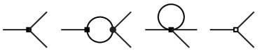
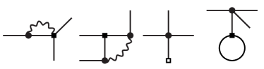
Figure 1: The diagrams for $K\to 2\pi$. An open square is a vertex from ${\cal L}_{W4}$ or ${\cal L}_{W2E2}$, a filled square a vertex from ${\cal L}_{W2}$ or ${\cal L}_{E2}\,(\Delta S=1)$ and a filled circle a vertex from ${\cal L}_{S2}$ or ${\cal L}_{E2}\,(\Delta S=0)$. A straight line is a pseudoscalar meson and a wiggly line a photon.

6.1.2 Next-to-leading Order

There are seven more diagrams contributing to next-to-leading order, see Fig. 1. The resulting amplitudes are long, and we decided to not include them here but instead make them available for download formulas . Note that we have also included contributions proportional to $G_{27}$, not included in k2piisofull . These are included for consistency between the $K\to 2\pi(\gamma)$ and $K\to 3\pi(\gamma)$ calculations.

6.2 $K\to 2\pi\gamma$

The amplitudes for the processes $K\to 2\pi\gamma$ have been calculated before. Here we only need the lowest order contribution to be consistent with the $K\to 2\pi$ calculation. This we recalculated and the starting point is the two diagrams that contribute to the process, shown in Fig. 2.

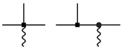
Figure 2: The diagrams for $K\to 2\pi\gamma$. A square is a weak vertex, a circle a strong vertex, a straight line a pseudoscalar meson and a wiggly line a photon.

Since photons at this order only couple to charged particles, there are only two different amplitudes and the results are

$$A^{S}_{+-\gamma} = e\,F\,\left(G_{8}+\frac{2}{3}\,G_{27}\right)\,(m_{K}^{2}-m_{\pi}^{2})$$

$$\left[-k.\varepsilon\,\left(\frac{1}{r_{1}}-\frac{1}{r_{2}}\right)+(p_{2}.\varepsilon\,-p_{1}.\varepsilon)\left(\frac{1}{r_{1}}+\frac{1}{r_{2}}\right)\right]\,,$$

and

$$A_{+0\gamma} = e\,F\,\frac{5}{6}\,G_{27}\,(m_{K}^{2}-m_{\pi}^{2})\,\left[-k.\varepsilon\,\left(\frac{1}{r_{0}}+\frac{1}{r_{1}}\right)\right.$$ (44)

$$\left.+p_{1}.\varepsilon\,\left(-\frac{1}{r_{0}}-\frac{1}{r_{1}}\right)+p_{2}.\varepsilon\,\left(-\frac{1}{r_{0}}+\frac{1}{r_{1}}\right)\right]\,.$$

These amplitudes can be decomposed into an electric and a magnetic part:

$$A(K\to 2\pi\gamma)=e\,\varepsilon^{\mu}(k)\,(E_{\mu}+\varepsilon_{\mu\nu\rho\sigma}M^{\nu\rho\sigma})\,,$$ (45)

but at lowest order the magnetic amplitude $M^{\nu\rho\sigma}$ vanishes since there is no $\varepsilon_{\mu\nu\rho\sigma}$ tensor in the corresponding lowest order Lagrangian.

The electric amplitude, on the other hand, is completely determined by the corresponding non-radiative amplitude via Low’s theorem Low58 .

6.3 $K\to 3\pi\gamma$

The decay $K\to 3\pi\gamma$ is discussed in detail in K3PG . We only need the lowest order amplitude for consistency with the calculation of $K\to 3\pi$. We have calculated the four different amplitudes using Chiral Perturbation Theory, and checked that they agree with Low’s theorem. The calculation is based on seven diagrams, see Fig. 3.

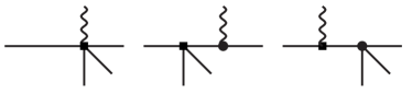
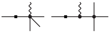
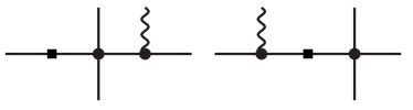
Figure 3: The diagrams for $K\to 3\pi\gamma$. A square is a weak vertex, a circle a strong vertex, a straight line a pseudoscalar meson and a wiggly line a photon.

The four amplitudes are

$$A^{L}_{+-0\gamma} = i\,e\,\left[\frac{G_{8}-G_{27}}{3}\,m_{K}^{2}+\right.$$ (46)

$$\left(-\frac{G_{8}}{3}-\frac{G_{27}}{6}\,\frac{-3\,m_{K}^{2}+8\,m_{\pi}^{2}}{m_{\pi}^{2}-m_{K}^{2}}\right)\times$$

$$(-3\,(s_{3\gamma}-2\,t_{1}-2\,t_{2})+m_{K}^{2}+3\,m_{\pi}^{2})\times$$

$$\,\left(\frac{p_{1}\cdot\varepsilon}{t_{1}}-\frac{p_{2}\cdot\varepsilon}{t_{2}}\right)$$

$$-6\,\left(-\frac{G_{8}}{3}-\frac{G_{27}}{6}\,\frac{-3\,m_{K}^{2}+8\,m_{\pi}^{2}}{m_{\pi}^{2}-m_{K}^{2}}\right)\times$$

$$(t_{2}+t_{1})\,\left(\frac{p_{1}\cdot\varepsilon}{t_{1}}-\frac{p_{2}\cdot\varepsilon}{t_{2}}\right)\Bigg{]}\,,$$

$$A^{S}_{+-0\gamma} = i\,e\,\frac{5}{6}\,\left(-\frac{G_{27}}{m_{\pi}^{2}-m_{K}^{2}}\right)\,(2\,m_{\pi}^{2}-3\,m_{K}^{2})\times$$ (47)

$$\left[(s_{1\gamma}-s_{2\gamma})\,\left(\frac{p_{1}\cdot\varepsilon}{t_{1}}-\frac{p_{2}\cdot\varepsilon}{t_{2}}\right)\right.$$

$$+2\,t_{0}\,\left(\frac{p_{1}\cdot\varepsilon}{t_{1}}+\frac{k\cdot\varepsilon}{t_{0}}\right)$$

$$+2\,t_{0}\,\left(\frac{p_{2}\cdot\varepsilon}{t_{2}}+\frac{k\cdot\varepsilon}{t_{0}}\right)\Bigg{]}\,,$$

$$A_{00+\gamma} = i\,e\,\left[-\frac{G_{8}}{2}\,(m_{K}^{2}+m_{\pi}^{2})-\frac{G_{27}}{m_{\pi}^{2}-m_{K}^{2}}\,(5/3\,m_{\pi}^{2}\,m_{K}^{2}\right.$$ (48)

$$-13/6\,m_{\pi}^{4}+1/2\,m_{K}^{4})-\left(\frac{G_{8}}{2}+\frac{G_{27}}{m_{\pi}^{2}-m_{K}^{2}}\times\right.$$

$$(7/6\,m_{\pi}^{2}-17/6\,m_{K}^{2})\Big{)}\,\times$$

$$(2\,(s_{3\gamma}-2\,t_{1}-2\,t_{2})-m_{K}^{2}-3\,m_{\pi}^{2})$$

$$-\frac{G_{27}}{m_{\pi}^{2}-m_{K}^{2}}\,5/6\,(2\,m_{\pi}^{2}-3\,m_{K}^{2})\times$$

$$(-(s_{3\gamma}-2\,t_{1}-2\,t_{2})+m_{K}^{2}+3\,m_{\pi}^{2})\Bigg{]}\times$$

$$\,\left(\frac{k\cdot\varepsilon}{t_{0}}+\frac{p_{3}\cdot\varepsilon}{t_{3}}\right)$$

$$A_{++-\gamma} = i\,e\,\Bigg{[}\Bigg{(}-G_{8}\,(m_{\pi}^{2}+m_{K}^{2})+G_{27}\,(m_{K}^{2}+13/3\,m_{\pi}^{2})$$

$$+(G_{8}-13/3\,G_{27})(s_{3\gamma}-2\,t_{1}-2\,t_{2})\Bigg{)}\times$$

$$\left(\frac{k\cdot\varepsilon}{t_{0}}+\frac{p_{1}\cdot\varepsilon}{t_{1}}+\frac{p_{2}\cdot\varepsilon}{t_{2}}-\frac{p_{3}\cdot\varepsilon}{t_{3}}\right)$$

$$+(2G_{8}-26/3\,G_{27})\,(t_{2}-t_{1})\left(\frac{p_{1}\cdot\varepsilon}{t_{1}}-\frac{p_{2}\cdot\varepsilon}{t_{2}}\!\right)\!\Bigg{]}.$$

Once again, these amplitudes can be decomposed into an electric and a magnetic part:

$$A(K\to 3\pi\gamma)=e\,\varepsilon^{\mu}(k)\,(E_{\mu}+\varepsilon_{\mu\nu\rho\sigma}M^{\nu\rho\sigma})\,,$$ (50)

and the magnetic amplitude $M^{\nu\rho\sigma}$ vanishes for the reasons given above.

The electric amplitude at this order is again completely determined by the corresponding non–radiative amplitude $A(s,\nu)$ via Low’s theorem Low58 ; K3PG :

$$E^{\mu} = A(s,\nu)\,\Sigma^{\mu}$$ (51)

$$\mbox{}+2\frac{\partial A(s,\nu)}{\partial s}\Lambda^{\mu}_{12}+\frac{\partial A(s,\nu)}{\partial\nu}(\Lambda^{\mu}_{14}-\Lambda^{\mu}_{24})$$

$$\mbox{}+{\cal O}(k)$$

with (the meson charges in units of $e$ are denoted $q_{i}$, with $\sum_{i=1}^{4}q_{i}=0$)

$$s = (p_{1}+p_{2})^{2}$$

$$\nu = k\cdot(p_{1}-p_{2})$$

$$\Sigma^{\mu} = \sum_{i=1}^{4}\frac{q_{i}p_{i}^{\mu}}{t_{i}}$$

$$\Lambda^{\mu}_{ij} = \Lambda^{\mu}_{ji}=(q_{i}t_{j}-q_{j}t_{i})D^{\mu}_{ij}$$

$$D^{\mu}_{ij} = -D^{\mu}_{ji}=\frac{p_{i}^{\mu}}{t_{i}}-\frac{p_{j}^{\mu}}{t_{j}}~{}.$$ (52)

Since there are no terms of ${\cal O}(k)$ at lowest order in the chiral expansion, the leading–order electric amplitude is completely determined by the explicit terms in (51).

7 Numerical Results

7.1 Experimental Data and Input

For the numerical studies we use the input given in Table 1.

$G_{E}$	$-0.4$	$L_{1}^{r}$	$0.38\cdot 10^{-3}$
$\sin\epsilon$	$1.19\cdot 10^{-2}$	$L_{2}^{r}$	$1.59\cdot 10^{-3}$
$Z$	$0.805$	$L_{3}^{r}$	$-2.91\cdot 10^{-3}$
$F_{\pi}$	$0.0924$ GeV	$L_{4}^{r}$	$0$
$F_{K}$	$0.113$ GeV	$L_{5}^{r}$	$1.46\cdot 10^{-3}$
$N_{14}$	$-10.4\cdot 10^{-3}$	$L_{6}^{r}$	$0$
$N_{15}$	$5.95\cdot 10^{-3}$	$L_{7}^{r}$	$-0.49\cdot 10^{-3}$
$D_{13}$	$0$	$L_{8}^{r}$	$1.0\cdot 10^{-3}$
$D_{15}$	$0$	$L_{9}^{r}$	$7.0\cdot 10^{-3}$

Table 1: The various input values used, LECs given at $\mu=0.77$ GeV.

7.1.1 Strong and Electromagnetic Input

There are different ways to treat the masses, especially in the isospin limit case. In BDP the masses used in the phase space were obtained from the physical masses occurring in the decays. However, in the amplitudes the physical mass of the kaon involved in the process was used and the pion mass was given by $m_{\pi}^{2}=\frac{1}{3}\sum_{i=1,3}m_{\pi^{i}}^{2}$ with $i=1,2,3$ being the three pions participating in the reaction. This allowed for the correct kinematical relation $s_{1}+s_{2}+s_{3}=m_{K}^{2}+3m_{\pi}^{2}$ to be satisfied while having the isospin limit in the amplitude but the physical masses in the phase space. The results in BDP were obtained with the physical mass for the eta. Results with the Gell-Mann-Okubo (GMO) relation for the eta mass in the loops gave small changes within the general errors given in BDP .

In the decays here, we work to first order in isospin breaking. We have rewritten explicit factors of $m_{u}-m_{d}$ in terms of $\sin\epsilon$ according to

$$m_{u}-m_{d}=-\frac{1}{\sqrt{3}}\,\,(2\,m_{s}-m_{u}-m_{d})\,\sin\epsilon\,.$$ (53)

In general we use the physical masses of pions and kaons in the loops but as soon as a factor of $\sin\epsilon$ or $e^{2}$ is present we use a common kaon and a common pion mass. This simplifies the analytical formulae enormously. The kaon mass chosen is the mass from the kaon in the decay and the pion mass used is $3m_{\pi}^{2}=\sum_{i}m_{\pi^{i}}^{2}$ with $i=1,2,3$ the three pions in the final state, i.e. the mass we used in the isospin limit case. For the eta mass we use in general the physical mass in the loop integrals. We have used the GMO mass relation with isospin violation included,

$$m_{\eta}^{2}=\frac{2}{3}\,(m_{K^{+}}^{2}+m_{K^{0}}^{2}-m_{\pi^{+}}^{2})+\frac{1}{3}\,m_{\pi^{0}}^{2}\,,$$ (54)

to simplify the amplitudes, except in the loops as stated above. The possible lowest order contributions from the eta mass have been removed from the amplitudes using the corresponding next-to-leading order relation as described in BB .

The strong LECs, $L_{1}^{r}$ to $L_{8}^{r}$, as well as $\sin\epsilon$ come from the one-loop fit in strongiso , $L_{9}^{r}$ from L9 and the $G_{E}$ estimate is from BP .

The constant $Z$ from ${\cal L}_{E2}$ we estimate via

$$Z=\frac{1}{2\,F_{\pi}^{2}\,e^{2}}\,(m_{\pi^{+}}^{2}-m_{\pi^{0}}^{2}),$$ (55)

which corresponds to the value in Table 1. The higher order coefficients of ${\cal L}_{E4}$, $K_{1}^{r}\ldots K_{12}^{r}$, are rather unknown. Some rough estimates exist but we put them to zero here, at the relevant scale.

The IR divergences are canceled by adding the soft-photon Bremsstrahlung. We have used a 1 MeV cut-off in energy for this and used the same cut-off in the definition of $F_{\pi^{+}}$ and $F_{K^{+}}$. We also use $m_{\gamma}=$ 1 MeV, which effectively removes the infrared part.

The subtraction scale $\mu$ is chosen to be $0.77$ GeV unless stated otherwise.

7.1.2 Input Relevant for the Photon Reducible Diagrams

The two constants $D_{13}$ and $D_{15}$ are set to zero since no knowledge exist of their values. One can determine the constants $N_{14}$ and $N_{15}$ from $K\to\pi l^{+}l^{-}$ decays. For a detailed analysis, see BB2 . The resulting values are given in Table 1. Note however, that as described in BB2 , $D_{13}$, $D_{15}$, $N_{14}$ and $N_{15}$ only contributes via the photon reducible diagrams. These diagrams are negligible numerically, unless the constants are orders of magnitude larger than expected.

7.2 Bremsstrahlung and Dependence on $m_{\gamma}$ and $\omega$

The isospin breaking amplitudes for $K\to 2\pi$ and $K\to 3\pi$ both depend on $m_{\gamma}$, introduced to regularize the infrared divergences coming from loops containing photons. This $m_{\gamma}$-dependence is canceled by adding the bremsstrahlung amplitudes, where a real soft photon is radiated off one of the mesons. This cancellation was checked for $K\to 3\pi$ in BB2 , and we have now also checked it for $K\to 2\pi$.

However, after the addition of bremsstrahlung the decay rates depend instead on $\omega$, the cut-off energy of the radiated real photon. This is a parameter that should be set to a value depending on the experiment that one compares to.

Another possibility, which we use in this paper, is to add the full amplitudes with an extra radiated photon, $K\to 2\pi\gamma$ and $K\to 3\pi\gamma$. When doing that the decay rates should be independent of $\omega$. We have checked this numerically and the results are presented in Table 2. For this comparison we have chosen $m_{\gamma}=0.1$ MeV and varied omega over a large range. One can see that up to photon energies of 1 MeV, the sum is constant within the expected uncertainties. The different sum when including energies up to 10 MeV is an indication that the soft photon approximation, used in calculating the infrared contribution, is breaking down.

$\omega\,(\mathrm{GeV})$	IR photon	Extra photon	$\mathrm{Sum}\,(\mathrm{GeV})$
	$(\mathrm{GeV})$	$(\mathrm{GeV})$
$K_{S}\to\pi^{+}\pi^{-}$
0.01	$4.34\cdot 10^{-17}$	$1.59\cdot 10^{-17}$	$5.92\cdot 10^{-17}$
0.001	$2.17\cdot 10^{-17}$	$3.69\cdot 10^{-17}$	$5.86\cdot 10^{-17}$
0.0005	$1.52\cdot 10^{-17}$	$4.34\cdot 10^{-17}$	$5.85\cdot 10^{-17}$
0.0001	$0$	$5.85\cdot 10^{-17}$	$5.85\cdot 10^{-17}$
$K^{+}\to\pi^{+}\pi^{0}$
0.01	$4.30\cdot 10^{-20}$	$1.54\cdot 10^{-20}$	$5.84\cdot 10^{-20}$
0.001	$2.15\cdot 10^{-20}$	$3.61\cdot 10^{-20}$	$5.77\cdot 10^{-20}$
0.0005	$1.50\cdot 10^{-20}$	$4.26\cdot 10^{-20}$	$5.76\cdot 10^{-20}$
0.0001	$0$	$5.77\cdot 10^{-20}$	$5.77\cdot 10^{-20}$
$K_{L}\to\pi^{+}\pi^{-}\pi^{0}$
0.01	$2.39\cdot 10^{-21}$	$3.39\cdot 10^{-22}$	$2.73\cdot 10^{-21}$
0.001	$1.19\cdot 10^{-21}$	$1.39\cdot 10^{-21}$	$2.58\cdot 10^{-21}$
0.0005	$8.34\cdot 10^{-22}$	$1.74\cdot 10^{-21}$	$2.58\cdot 10^{-21}$
0.0001	$0$	$2.56\cdot 10^{-21}$	$2.56\cdot 10^{-21}$
$K_{S}\to\pi^{+}\pi^{-}\pi^{0}$
0.01	$5.88\cdot 10^{-24}$	$8.93\cdot 10^{-25}$	$6.77\cdot 10^{-24}$
0.001	$2.94\cdot 10^{-24}$	$3.43\cdot 10^{-24}$	$6.37\cdot 10^{-21}$
0.0005	$2.05\cdot 10^{-24}$	$4.28\cdot 10^{-24}$	$6.34\cdot 10^{-21}$
0.0001	$0$	$6.29\cdot 10^{-24}$	$6.29\cdot 10^{-24}$
$K^{+}\to\pi^{0}\pi^{0}\pi^{+}$
0.01	$3.77\cdot 10^{-22}$	$4.03\cdot 10^{-23}$	$4.18\cdot 10^{-22}$
0.001	$1.89\cdot 10^{-22}$	$1.98\cdot 10^{-22}$	$3.86\cdot 10^{-22}$
0.0005	$1.32\cdot 10^{-22}$	$2.53\cdot 10^{-22}$	$3.85\cdot 10^{-22}$
0.0001	$0$	$3.83\cdot 10^{-22}$	$3.83\cdot 10^{-22}$
$K^{+}\to\pi^{+}\pi^{+}\pi^{-}$
0.01	$5.05\cdot 10^{-21}$	$5.86\cdot 10^{-22}$	$5.63\cdot 10^{-21}$
0.001	$2.52\cdot 10^{-21}$	$2.73\cdot 10^{-21}$	$5.25\cdot 10^{-21}$
0.0005	$1.76\cdot 10^{-21}$	$3.46\cdot 10^{-21}$	$5.23\cdot 10^{-21}$
0.0001	$0$	$5.19\cdot 10^{-21}$	$5.19\cdot 10^{-21}$

Table 2: $K\to 2,3\pi$ decay rates calculated for different values on $\omega$. Here we use $m_{\gamma}=$ 0.1 MeV and the same value is used as a cut-off in the decay constants, see the appendix in BB2 .

The way we treated the Bremsstrahlung contribution in the fits is as follows. We assume that the measured decay widths are including all photons. To compare to our amplitudes (calculated without hard photons), we therefore subtract numerically the calculated hard photon contributions from the experimental numbers.

7.3 Fit to $K\to 2\pi$

The process $K\to 2\pi$ in the presence of isospin breaking has been discussed in detail in k2piisofull . We have reproduced that calculation but added in addition also all the isospin breaking contributions from the 27 amplitudes, except for the parts from the weak-electromagnetic 27 Lagrangian.

The isospin breaking corrections to the decay rates are rather small, but they have an impact on the phase shift between the $I=2$ and $I=0$ amplitudes, $\delta_{2}-\delta_{0}$, as described in detail in k2piisofull . Our results are compatible with the ones presented there. The phase shift we use here is defined via

$$A^{S}_{00} = \frac{\sqrt{2}}{\sqrt{3}}A_{0}-\frac{2}{\sqrt{3}}A_{2}\,,$$

$$A^{S}_{+-} = \frac{\sqrt{2}}{\sqrt{3}}A_{0}+\frac{1}{\sqrt{3}}A_{2}\,,$$

$$A_{+0} = \frac{\sqrt{3}}{2}A_{2}^{+}\,,$$

$$\frac{A_{2}}{A_{0}} = \left|\frac{A_{2}}{A_{0}}\right|e^{i(\delta_{2}-\delta_{0})}\,.$$ (56)

In the fits we have left $\delta_{2}-\delta_{0}$ as an additional free parameter, as it is known that this phase is badly reproduced at one-loop order in ChPT. Note that because of the isospin breaking the $A_{2}^{+}$ amplitude is different from $A_{2}$.

We have performed a lowest order and a NLO fit to only the $K\to 2\pi$ amplitudes. In the NLO fit we set all the extra parameters, $\tilde{K}_{i}=K_{i}^{r}=Z_{i}^{r}=0$ at the scale $\mu$ indicated. The Bremsstrahlung contribution has been subtracted as discussed above.

$K\to 2\pi$
Order	$\mu$ [GeV]	$G_{8}$	$G_{27}$	$\delta_{2}-\delta_{0}$
LO		10.4	0.55	$-60.3\,^{\circ}$
NLO	0.6	6.43	0.44	$-58.9\,^{\circ}$
NLO	0.77	5.39	0.36	$-58.0\,^{\circ}$
NLO	1.0	4.60	0.30	$-57.4\,^{\circ}$

Table 3: Quantities fitted from $K\to 2\pi$ only. The scale $\mu$ is the scale at which the unknown low energy constants are put to zero.

As can be seen in Table 3, there is a sizable variation depending on the input scale used. There is very little change in the absolute values of $G_{8}$ and $G_{27}$ compared to the isospin limit fit of BDP , where only the fit with $\mu=0.77$ GeV was done. The angle is similar to the fit there, but this is a combination of two different effects. It was lowered because the new KLOE data have now been included in the PDG averaging, but the isospin breaking effects induced a positive correction as was also found in k2piisofull .

The values of $G_{8}$ and $G_{27}$ are determined by fitting $CF_{0}^{4}G_{8}$ and $CF_{0}^{4}G_{27}$ and then setting $F_{0}=F_{\pi}$ numerically to provide the numbers in the tables.

7.4 Fit to $K\to 2\pi$ and $K\to 3\pi$

Decay	Width [GeV]	ChPT [GeV]	Fact. [GeV]
$K^{+}\to\pi^{+}\pi^{0}$	$(1.1231\pm 0.0078)\cdot 10^{-17}$	$1.123\cdot 10^{-17}$	$1.127\cdot 10^{-17}$
$K_{S}\to\pi^{0}\pi^{0}$	$(2.2828\pm 0.0104)\cdot 10^{-15}$	$2.282\cdot 10^{-15}$	$2.283\cdot 10^{-15}$
$K_{S}\to\pi^{+}\pi^{-}$	$(5.0691\pm 0.0108)\cdot 10^{-15}$	$5.069\cdot 10^{-15}$	$5.069\cdot 10^{-15}$
$K_{L}\to\pi^{0}\pi^{0}\pi^{0}$	$(2.6748\pm 0.0358)\cdot 10^{-18}$	$2.618\cdot 10^{-18}$	$2.698\cdot 10^{-18}$
$K_{L}\to\pi^{+}\pi^{-}\pi^{0}$	$(1.5998\pm 0.0271)\cdot 10^{-18}$	$1.658\cdot 10^{-18}$	$1.711\cdot 10^{-18}$
$K^{+}\to\pi^{0}\pi^{0}\pi^{+}$	$(9.195\pm 0.0213)\cdot 10^{-19}$	$8.934\cdot 10^{-19}$	$8.816\cdot 10^{-19}$
$K^{+}\to\pi^{+}\pi^{+}\pi^{-}$	$(2.9737\pm 0.0174)\cdot 10^{-18}$	$2.971\cdot 10^{-18}$	$2.933\cdot 10^{-18}$

Table 4: The various decay widths from the PDG tables PDG , and our results from the main fit and the best factorization fit.

Decay	Quantity	Experiment	ChPT	Fact.
$K_{L}\to\pi^{0}\pi^{0}\pi^{0}$	$h$	$-0.0050\pm 0.0014$	-0.0062	-0.0025
$K_{L}\to\pi^{+}\pi^{-}\pi^{0}$	$g$	$0.678\pm 0.008$	0.678	0.654
	$h$	$0.076\pm 0.006$	0.088	0.083
	$k$	$0.0099\pm 0.0015$	0.0057	0.0068
$K_{S}\to\pi^{+}\pi^{-}\pi^{0}$	$\gamma_{S}$	$(3.3\pm 0.5)\cdot 10^{-8}$	$3.0\cdot 10^{-8}$	$2.9\cdot 10^{-8}$
$K^{\pm}\to\pi^{0}\pi^{0}\pi^{\pm}$	$g$	$0.638\pm 0.020$	0.636	0.648
	$h$	$0.051\pm 0.013$	0.077	0.080
	$k$	$0.004\pm 0.007$	0.0047	0.0069
$K^{+}\to\pi^{+}\pi^{+}\pi^{-}$	$g$	$-0.2154\pm 0.0035$	$-$0.215	$-$0.226
	$h$	$0.012\pm 0.008$	0.012	0.019
	$k$	$-0.0101\pm 0.0034$	$-$0.0034	$-$0.0033
$K^{-}\to\pi^{-}\pi^{-}\pi^{+}$	$g$	$-0.217\pm 0.007$
	$h$	$0.010\pm 0.006$
	$k$	$-0.0084\pm 0.0019$

Table 5: Experimental values and the main fit and best factorization fit of the Dalitz plot distribution parameters. The data are from the PDG tables PDG except $\gamma_{S}$ from CPLEAR .

The quantities we fit are the measured decay rates and the various parameters of the Dalitz plot distributions defined via

$$\left|\frac{A(s_{1},s_{2},s_{3})}{A(s_{0},s_{0},s_{0})}\right|^{2}=1+gy+hy^{2}+kx^{2}\,.$$ (57)

For the decay $K_{L}\to 3\pi^{0}$, $k=h/3$ and $g=0$. The decay $K_{s}\to\pi^{+}\pi^{-}\pi^{0}$ is included via

$$A^{S}_{+-0}=\gamma_{S}x-\xi xy\,.$$ (58)

The decay rates are included in the fit as follows. We subtract from the decay rates the Bremsstrahlung contributions as described above as a function of $G_{8}$ and $G_{27}$. We then convert the decay rate using the central values of the measured Dalitz plot distribution into a value for the amplitude squared at the center of the Dalitz plot. These squared amplitudes together with the parameters $g,h,k$ and $\gamma_{S}$ are used as the 18 experimental parameters to be fitted.

This means that the effect of Bremsstrahlung is included fully in the decay rates, but only via the soft photon approximation with a 1 MeV cut-off for the Dalitz plot distributions. We have not included the preliminary data from KTeV, NA48 and KLOE.

The number of free input parameters on the theory side is very large. Since it turns out that the isospin breaking effects are very small, we put those extra NLO parameters equal to zero at the scale $\mu$ indicated in the tables.

Let us repeat here the definitions of the various extra NLO parameters. The $L_{i}^{r}$ are taken from the standard fit done at one loop to be compatible with the order of this calculation. The $K_{i}^{r}$ are the extra parameters at NLO in the $p^{2}e^{2}$ sector. Those are always put to zero at the scale indicated. In the isospin limit 11 combinations of the weak NLO low-energy coefficients show up, as discussed in BDP . These are $\tilde{K}_{i}$, $i=1,\ldots,11$. In the presence of isospin breaking many more combinations of these, as well as from the weak octet order $e^{2}p^{2}$ Lagrangian, emerge and they were classified in BB . The 27-part of the weak Lagrangian of order $e^{2}p^{2}$ has not been worked out and will lead to some more free parameters. We have not used any estimates of these extra parameters but set all of them to zero at the scale indicated, except for $\tilde{K}_{i}$, $i=1,\ldots,7$. The reason for this choice is that they are the leading contributions. $\tilde{K}_{1,2,3}$ are octet enhanced and come multiplied with factors of order $m_{K}^{4}$ and $\tilde{K}_{4,5,6,7}$ are 27-plets but also come multiplied with factors of order $m_{K}^{4}$. The neglected ones are thus suppressed by either isospin breaking, factors of $m_{\pi}^{2}/m_{K}^{2}$ or by the $\Delta I=1/2$ rule, i.e. an extra factor of $G_{27}/G_{8}$.

7.4.1 General Fits

Here we perform the fits with similar assumptions as used in the isospin limit fit, as well as a few additional ones. First $G_{8}$ and $G_{27}$ are extremely correlated with the values of $\tilde{K}_{1}$ and $\tilde{K}_{4}$ respectively. They are very difficult to obtain separately without additional assumptions. The main fit is therefore the one with

$$\tilde{K}_{1}=\tilde{K}_{4}=\tilde{K}_{8}=\tilde{K}_{9}=0\,,$$ (59)

at a scale $\mu=0.77$ GeV. The results are given in Table 6. This table is very similar to Table 6 in BDP . The large values of $\tilde{K}_{6}$ and the resulting large value of $\tilde{K}_{7}$ have the same origin as in that reference. In order to fit $\gamma_{S}$ well, $\tilde{K}_{6}$ is put large because it gets multiplied there with a small factor and is the only one contributing. This in turn leads large values for $\tilde{K}_{7}$ to compensate in other places.

The fit with

$$\tilde{K}_{6}=0$$ (60)

in addition has only a slightly larger $\chi^{2}$ and a smaller $\tilde{K}_{7}$. The $\chi^{2}$ is larger than in BDP because the experimental errors on several quantities have decreased since then. The overall fit is slightly better than the one of BDP because the newer measurements of the Dalitz distribution in $K^{+}\to\pi^{0}\pi^{0}\pi^{+}$ agree better with the chiral expressions.

Constraint	Eq. (59)	Eq. (59)	Eq. (59)	Eq. (59,60)
$\mu$	0.77 GeV	1.0 GeV	0.6 GeV	0.77 GeV
$G_{8}$	5.39(1)	4.60(1)	6.43(1)	5.39(1)
$G_{27}$	0.359(2)	0.301(1)	0.438(2)	0.359(2)
$\delta_{2}-\delta_{0}$	$-57.(1.5)^{o}$	$-57.3(1.4)^{o}$	$-58.9(1.4)^{o}$	$-57.9(1.4)^{o}$
$10^{3}\tilde{K}_{1}/G_{8}$	$\equiv 0$	$\equiv 0$	$\equiv 0$	$\equiv 0$
$10^{3}\tilde{K}_{2}/G_{8}$	48.5(2.4)	56.5(2.4)	41.2(1.9)	46.6(1.6)
$10^{3}\tilde{K}_{3}/G_{8}$	2.6(1.2)	$-$1.7(1.1)	6.7(1.0)	3.5(0.8)
$10^{3}\tilde{K}_{4}/G_{27}$	$\equiv 0$	$\equiv 0$	$\equiv 0$	$\equiv 0$
$10^{3}\tilde{K}_{5}/G_{27}$	$-$41.2(16.9)	$-$52.0(17.7)	$-$31.1(12.0)	$-$27.0(8.3)
$10^{3}\tilde{K}_{6}/G_{27}$	$-$102(105)	$-$114(105)	$-93(76)$	$\equiv 0$
$10^{3}\tilde{K}_{7}/G_{27}$	78.6(33)	78.0(33.5)	79.6(22.7)	50.0(13.0)
$10^{3}\tilde{K}_{8}/G_{8}$	$\equiv 0$	$\equiv 0$	$\equiv 0$	$\equiv 0$
$10^{3}\tilde{K}_{9}/G_{8}$	$\equiv 0$	$\equiv 0$	$\equiv 0$	$\equiv 0$
$\chi^{2}$/DOF	29.3/10	27.2/10	33.0/10	30.5/11

Table 6: The results for $G_{8}$ and $G_{27}$ and the $\tilde{K}_{i}$ for the various constraints described in the text. In brackets are the MINUIT errors. The $\tilde{K}_{i}$ are quoted at the scale $\mu$ mentioned.

We get fits of roughly similar quality for all values of $\mu$ where the other parameters have been put to zero. The fits tend to be slightly better for the larger values of $\mu$. The fitted values for the $\tilde{K}_{i}$ are $\mu$-dependent, albeit not extremely strongly.

The $\tilde{K}_{i}$ themselves have a $\mu$-dependence which is given by the cancellation of divergences, and this can be calculated from the known subtractions. We have shown the variation with $\mu$ from $\mu=0.77~{}GeV$ to $\mu=0.6$ GeV and $\mu=1.0$ GeV for $\tilde{K}_{i}$, $i=1,\ldots,11$ in Table 7

In order to compare with the factorization model of the weak low energy constants, we also perform a fit where all next-to-leading order LECs proportional to $G_{27}$ are set to zero, but we keep in addition the sub-leading octet ones. This fit is shown for $\mu=0.77$ GeV in Table 7. The fit is somewhat worse than those of Tab. 6 but not much. A very similar fit is obtained for $\mu=1$ GeV with a $\chi^{2}$ of 29.9. At $\mu=0.6~{}GeV$ the best solution found had a $\chi^{2}$ of 57.8. This fit corresponds to

$$\tilde{K}_{4}=\tilde{K}_{5}=\tilde{K}_{6}=\tilde{K}_{7}=0\,,$$ (61)

and this type of fit is referred to below as an octet fit.

Constraint	Eq. (61)	$\mu$ variation	$\mu$ variation
$\mu$	0.77 GeV	1.0 GeV	0.6 GeV
$G_{8}$	4.84(1)	–	–
$G_{27}$	0.430(1)	–	–
$\delta_{2}-\delta_{0}$	$-57.9(0.2)^{o}$	–	–
$10^{3}\tilde{K}_{1}/G_{8}$	2.0(1)	$-$5.88	5.61
$10^{3}\tilde{K}_{2}/G_{8}$	63.0(1.5)	$-$2.69	2.57
$10^{3}\tilde{K}_{3}/G_{8}$	$-$6.0(7)	0.159	$-$0.152
$10^{3}\tilde{K}_{4}/G_{27}$	$\equiv 0$	$-$9.93	9.48
$10^{3}\tilde{K}_{5}/G_{27}$	$\equiv 0$	0	0
$10^{3}\tilde{K}_{6}/G_{27}$	$\equiv 0$	27.0	$-$25.8
$10^{3}\tilde{K}_{7}/G_{27}$	$\equiv 0$	$-$21.5	20.5
$10^{3}\tilde{K}_{8}/G_{8}$	20.4(1)	$-$0.546	0.521
$10^{3}\tilde{K}_{9}/G_{8}$	9.1(1)	$-$2.92	2.79
$10^{3}\tilde{K}_{10}/G_{8}$	$\equiv 0$	11.6	$-$11.1
$10^{3}\tilde{K}_{11}/G_{8}$	$\equiv 0$	$-$1.66	1.58
$\chi^{2}$/DOF	33.3/10	–	–

Table 7: The results for $G_{8}$ and $G_{27}$ and the $\tilde{K}_{i}$ for the octet constraint described in the text. In brackets are the MINUIT errors. The $\tilde{K}_{i}$ are quoted at the scale $\mu$ mentioned. The last two columns are the values of the $\tilde{K}_{i}$ at the scale $\mu$ mentioned when they are zero at $\mu=0.77~{}GeV$ and run with $G_{8}=5.39$ and $G_{27}=0.359$.

7.4.2 Fits to Factorization and other Models

Various models for the NLO weak constants exist. We will discuss here some of the ones which are presented in EKW . These have been discussed in that reference only for the pure octet case. So the quality of the models should be compared with the octet fit above.

A first choice is the resonance exchange domination of the weak constants. The problem here is that the weak decays of the resonances involve themselves many new unmeasured parameters and thus leads to fairly few general conclusions. If we assume that the vector octet exchange dominates, we get a relation between the octet NLO constants

$$N_{1}^{r}+N_{2}^{r}+2N_{3}^{r}=0\,,$$ (62)

which is a combination we can in fact determine. It translates for our parameters into

$$\tilde{K}_{3}=-\frac{1}{2}\tilde{K}_{2}\,.$$ (63)

It can be easily seen from Tables 6 and 7 that this is very far from being satisfied by our fits.

A very often used model is the factorization model. It corresponds to taking the underlying four quark operator and bosonizing separately the two quark currents present there. Looking at the dominant octet operators only for the cases that we need here, this leads to the relations EKW

$$N_{1}^{r} = 2k_{f}(32/3\,L_{1}^{r}+4\,L_{3}^{r}+2/3\,L_{9}^{r})\,,$$

$$N_{2}^{r} = 2k_{f}(16/3L_{1}^{r}+4L_{3}^{r}+10/3\,L_{9}^{r})\,,$$

$$N_{3}^{r} = 2k_{f}(8L_{2}^{r}-2L_{9}^{r})\,,$$

$$N_{4}^{r} = 2k_{f}(-16/3\,L_{1}^{r}-8/3\,L_{3}^{r}-4/3\,L_{9}^{r})\,,$$

$$N_{5}^{r} = 2k_{f}(-L_{5}^{r})\,,$$

$$N_{6}^{r} = 2k_{f}(2/3\,L_{5}^{r})\,,$$

$$N_{7}^{r} = 2k_{f}(L_{5}^{r})\,,$$

$$N_{8}^{r} = 2k_{f}(4\,L_{4}^{r}+2\,L_{5}^{r})\,,$$

$$N_{9}^{r} = N_{10}^{r}=N_{11}^{r}=N_{12}^{r}=N_{13}^{r}=0\,.$$ (64)

The parameter $k_{f}$ allows for some overall adjustment. The special value $k_{f}=1/2$ is referred to as the Weak Deformation Model (WDM)EKW ; EPR . We have performed a fit leaving both $k_{f}$ and $\mu$ free. Note that the scale $\mu$ is also the scale where we have put all the other NLO parameters equal to zero. The input values of the $L_{i}^{r}$ have been scaled accordingly.

The fits done with $k_{f}$, $G_{8}$ and $G_{27}$ as free parameters have $\chi^{2}$ significantly larger than those reported above. Some representative values are shown in Table 8.

The fit with $\mu$ free gave a minimum at $\mu=0.842$ GeV. The fits with $\mu$ outside the range of Table 8 had very large values of $\chi^{2}$.

$\mu$	0.77 GeV	0.9 GeV	0.842 GeV
$G_{8}$	4.18(1)	4.42	4.22(1)
$G_{27}$	0.360(2)	0.326(10)	0.339(10)
$k_{F}$	2.61(1)	4.94(2)	3.60(5)
$\chi^{2}$/DOF	109/14	182/14	60.4/13

Table 8: The results for the fit with the factorization assumption for various values of $\mu$ including the optimal one.

In order to show the quality of the fits we have given in Tables 4 and 5 also the values obtained for the quantities from the main fit and best factorization fit, labeled ChPT and Fact. respectively. Notice that the extrapolation to the full phase space here has been done from the amplitude squared in the center of the Dalitz plot using the experimental values for the distribution over the Dalitz plot.

8 Summary

We have recalculated in this paper the Bremsstrahlung amplitudes for $K\to 2\pi\gamma$ and $K\to 3\pi\gamma$. In addition we have calculated also the isospin violating effects to $K\to 2\pi$ including those with the 27-operators both for effects due to $m_{u}-m_{d}$ and electromagnetism. This we did to be consistent with the calculations of $K\to 3\pi$ done in BB ; BB2 .

We have checked explicitly that the infrared divergences of the photon loops regulated by $m_{\gamma}$ cancel between the virtual photon loops and the soft Brems-strahlung. We checked in addition that the photon energy cut-off dependence cancels between the soft-photon Bremsstrahlung part and the part where hard photons are treated explicitly. We have not included the explicit expressions for the $K\to 2\pi$ amplitudes because they are rather long. They can be obtained from the authors or formulas . These amplitudes have passed all the standard tests, like cancellation of divergences from both NLO ChPT as well as the infrared singularities.

With these calculations and those published earlier in BB ; BB2 , we have updated the fit to the CP conserving observables in the $K\to\pi\pi(\pi)(\gamma)$ system done in the isospin limit in BDP . As expected from the fairly small isospin violating effects found in BB ; BB2 and from the analysis of isospin breaking effects in the $K\to\pi\pi(\gamma)$ system of k2piisofull , the differences with the isospin conserving case are rather small. In addition we have studied the dependences on the subtraction scale $\mu$, where the various assumptions are made. Our full amplitudes are $\mu$ independent as they should.

The fits show a similar quality to the ones performed earlier. The main differences are that the experimental Dalitz parameters have changed in $K^{+}\to\pi^{+}\pi^{+}\pi^{0}$ and are now in better agreement with the ChPT fits. This is purely experimental and has nothing to do with the inclusion of isospin breaking effects. The total $\chi^{2}$ is somewhat worse because the experimental errors on various partial widths have been reduced.

We also checked how well a few models of the NLO weak low energy constants work. The dominance by vectors and the weak deformation model gave a rather bad fit. The factorization model gave a somewhat better fit when an extra parameter, an overall scale factor, was allowed. The quality of this compared to the optimal ChPT fits can be judged from the tables giving the best fit values for the experimental quantities directly.

References

- (1) S. Weinberg, Physica A 96 (1979) 327.
- (2) J. Gasser and H. Leutwyler, Annals Phys. 158 (1984) 142.
- (3) J. Gasser and H. Leutwyler, Nucl. Phys. B 250 (1985) 465.
-
(4)
A. Pich, Lectures at Les Houches Summer School in
Theoretical Physics, Session 68: Probing the Standard Model of Particle
Interactions, Les Houches, France, 28 Jul - 5 Sep 1997,
hep-ph/9806303;
G. Ecker, Lectures given at Advanced School on Quantum Chromodynamics (QCD 2000), Benasque, Huesca, Spain, 3-6 Jul 2000, hep-ph/0011026. - (5) J. Kambor, J. Missimer and D. Wyler, Nucl. Phys. B 346 (1990) 17.
- (6) J. Kambor, J. Missimer and D. Wyler, Phys. Lett. B 261 (1991) 496.
-
(7)
G. Ecker,
Prog. Part. Nucl. Phys. 35 (1995) 1,
[hep-ph/9501357];
A. Pich, Rept. Prog. Phys. 58 (1995) 563, [hep-ph/9502366];
E. de Rafael, Lectures given at Theoretical Advanced Study Institute in Elementary Particle Physics (TASI 94): CP Violation and the limits of the Standard Model, Boulder, CO, 29 May - 24 Jun 1994, hep-ph/9502254. - (8) J. Bijnens, E. Pallante and J. Prades, Nucl. Phys. B 521 (1998) 305, [hep-ph/9801326].
- (9) J. Bijnens, P. Dhonte and F. Persson, Nucl. Phys. B 648 (2003) 317, [hep-ph/0205341].
- (10) E. Gamiz, J. Prades and I. Scimemi, JHEP 0310 (2003) 042, [hep-ph/0309172].
- (11) J. Bijnens and F. Borg, Nucl. Phys. B 697 (2004) 319, [hep-ph/0405025].
- (12) I. Scimemi, E. Gamiz and J. Prades, Invited talk at 39th Rencontres de Moriond on Electroweak Interactions and Unified Theories, La Thuile, Aosta Valley, Italy, 21-28 Mar 2004, hep-ph/0405204.
- (13) J. Bijnens and F. Borg, hep-ph/0410333. To be published in Eur. Phys. J. C.
- (14) A. Nehme, Phys. Rev. D 70, 094025 (2004), [hep-ph/0406209].
- (15) I. V. Ajinenko et al., Phys. Lett. B 567, 159 (2003), [hep-ex/0205027].
- (16) A. Aloisio et al. [KLOE Collaboration], hep-ex/0307054.
- (17) N. Cabibbo, Phys. Rev. Lett. 93 (2004) 121801, [hep-ph/0405001].
- (18) G. Amorós, J. Bijnens, P. Talavera Nucl. Phys. B 602 (2001) 87, [hep-ph/0101127].
- (19) J. A. Cronin, Phys. Rev. 161 (1967) 1483.
- (20) G. Ecker, G. Isidori, G. Muller, H. Neufeld and A. Pich, Nucl. Phys. B 591 (2000) 419, [hep-ph/0006172].
- (21) V. Cirigliano, M. Knecht, H. Neufeld, H. Rupertsberger and P. Talavera, Eur. Phys. J. C 23, 121 (2002), [hep-ph/0110153].
- (22) G. Esposito-Farese, Z. Phys. C 50 (1991) 255.
- (23) G. Ecker, J. Kambor and D. Wyler, Nucl. Phys. B 394 (1993) 101, [hep-ph/0006172].
- (24) R. Urech, Nucl. Phys. B 433, 234 (1995), [hep-ph/9405341].
- (25) V. Cirigliano, G. Ecker, H. Neufeld and A. Pich, Eur. Phys. J. C 33 (2004) 369, [hep-ph/0310351].
-
(26)
J. Bijnens and M. B. Wise,
Phys. Lett. B 137 (1984) 245;
B. R. Holstein, Phys. Rev. D 20 (1979) 1187;
S. Gardner and G. Valencia, Phys. Rev. D 62 (2000) 094024, [hep-ph/0006240],
C. E. Wolfe and K. Maltman, Phys. Lett. B 482 (2000) 77, [hep-ph/9912254];
V. Cirigliano, J. F. Donoghue and E. Golowich, Phys. Lett. B 450 (1999) 24,
V. Cirigliano, J. F. Donoghue and E. Golowich, Eur. Phys. J. C 18 (2000) 83, [hep-ph/0008290],
G. Ecker, G. Muller, H. Neufeld and A. Pich, Phys. Lett. B 477 (2000) 88, [hep-ph/9912264];
-
(27)
These can be downloaded
from
http://www.thep.lu.se/~bijnens/chpt.html. - (28) F.E. Low, Phys. Rev. 110 (1958) 974.
- (29) G. D’Ambrosio, G. Ecker, G. Isidori and H. Neufeld, Z. Phys. C 76 (1997) 301, [hep-ph/9612412].
- (30) J. Bijnens and P. Talavera, JHEP 0203 (2002) 046, [hep-ph/0203049].
- (31) J. Bijnens and J. Prades, JHEP 0006 (2000) 035, [hep-ph/0005189].
- (32) S. Eidelman et al. [Particle Data Group Collaboration], Phys. Lett. B 592, 1 (2004).
-
(33)
R. Adler et al. [CPLEAR Collaboration],
Phys. Lett. B 407 (1997) 193;
R. Adler et al. [CPLEAR Collaboration], Phys. Lett. B 374 (1996) 313;
A. Angelopoulos et al. [CPLEAR Collaboration], Eur. Phys. J. C 5 (1998) 389. - (34) G. Ecker, A. Pich and E. de Rafael, Nucl. Phys. B 291 (1987) 692.
- (35) J. A. Vermaseren, math-ph/0010025.