Lepton Flavor Violation in Extra Dimension Models

Abstract

Models involving large extra spatial dimension(s) have interesting predictions on lepton flavor violating processes. We consider some 5D models which are related to neutrino mass generation or address the fermion masses hierarchy problem. We study the signatures in low energy experiments that can discriminate the different models. The focus is on muon-electron conversion in nuclei, $\mu\rightarrow e\gamma$ and $\mu\rightarrow 3e$ processes and their $\tau$ counterparts. Their links with the active neutrino mass matrix are investigated. We show that in the models we discussed the branching ratio of $\mu\rightarrow e\gamma$ like rare process is much smaller than the ones of $\mu\rightarrow 3e$ like processes. This is in sharp contrast to most of the traditional wisdom based on four dimensional gauge models. Moreover, some rare tau decays are more promising than the rare muon decays.

I Introduction

In the Standard Model(SM) with fifteen fermions per family neutrinos are strictly massless and the charged leptons’ weak eigenstates can be chosen to be their mass eigenstates. Thus, each generation has a separately conserved lepton number. If one neglects the tiny effects from nonperturbative processes, there is no lepton flavor violating(LFV) interaction in SM. However, recent neutrino experiments show strong evidence that neutrinos have none zero masses and the three active neutrinos mixSuperK ; SNO ; KamL ; WMAP . Most physicists take this to be a harbinger of new physics beyond the SM. Moreover, finite neutrino masses alone would imply the existence of LFV in charged lepton sector analogous to the quarks. If so we expect the Glashow-Iliopoulos-Maiani(GIM) mechanism to be operative in the lepton sector then the rate of induced LFV processes will be proportional to the neutrino mass square difference, which is of the order of $<10^{-3}(eV)^{2}$. Hence, they will be hopelessly small for experimental verification. Therefore, additional ingredients are essential for a detectable LFV signature. It is very common in model building to have the new physics that generate neutrino masses also given rise to LFV reactions. This link appears to be natural although there is no guarantee that this is case in nature. With this cautionary note we will focus attention to new physics that links the two phenomena.

Among the numerous beyond the SM models, LFV signatures are most intensely studied in supersymmetric (SUSY) ones. The connection with neutrino masses is established through the seesaw mechanism which is the orthodox way of getting a small mass for the active neutrinos. Since the latter has a natural setting in grand unified theories (GUT) the end result are rather bedecked supersymmetric seesaw models; see e.g. susylfv . Although the details are different the generic source of LFV lies in the mixing of various sfermions. The right-handed Majorana neutrinos play a secondary role in this class of models. In general it is natural to expect $B(\mu\rightarrow e\gamma)\gg B(\mu\rightarrow 3e)$ in SUSY models.

For non-supersymmetric models neutrino mass generation via the seesaw mechanism would required the right-handed neutrinos to be of the GUT scale. In this simplest version all LFV are undetectable. Attempts are now made to lower some right-handed neutrinos mandated by the seesaw mechanism to the TeV scale so that the seesaw mechanism itself can be tested experimentally. If so then one can optimistically anticipate LFV signatures in the next round of experiments CN04 . Independent of the details of the models one again expects $B(\mu\rightarrow e\gamma)\gg B(\mu\rightarrow 3e)$ to hold true.

Recently a new avenue has open up in the construction of models beyond the SM that exploits the possible existence of extra spatial dimensions. These theories are particularly interesting phenomenologically in the brane world context. It is fascinating that many long standing problems in the usual four dimensional (4D) field theories can be overcome or take on new perspectives in these higher dimensional constructs. For example the hierarchy problem is solved by invoking large extra dimensions. In this note, we would like to draw the readers’ attention to the models which involve one or more flat extra spatial dimensions. Furthermore, we focus on those that address the neutrino mass problem. In some cases, we predict a reversed pattern of $B(\mu\rightarrow 3e)\gg B(\mu\rightarrow e\gamma)$ compare to SUSY models. On the experimental side, it shall be interesting to see this.

The current experimental limits on muon LFV have already put very stringent constraints on model building. On the other hand, the limits from tau LFV are rather loose. We shall constraint the extra dimension models by the muon rare processes data and place upper limits on the rare decays of the $\tau$. To avoid any hadronic uncertainties we shall focus on purely leptonic processes. We shall also discuss the possible ways to discriminate different models and their connections to neutrino masses.

In this brief review, we give few examples of extra dimension models which give potentially testable LFV signatures. These LFV processes are all directly or indirectly related to the generation of neutrino masses. We compare the LFV processes in a five dimension(5D) $SU(3)_{W}$SU3:triumf and $SU(5)$SU5:triumf GUT models where neutrino Majorana masses are generated radiatively without a right-handed neutrino which is viable but less discussed alternative to the seesaw mechanism. A brief review of this construction is given in JN . Also, we discuss the LFV processes in split fermion or multi-brane scenario.

The following is our plan for the paper. In sec.II, we will first review the general operator analysis for the lepton flavor violating processes. This will also set the notations for the rest of the discussions. Sec. III examines LFV in a 5D $SU(3)_{w}$ model. New results of the one-loop calculations are given here. For details of the model and neutrino mass generation we refer to SU3:triumf . In Sec. IV, the LFV processes induced by 5D $SU(5)$ model will be discussed. The discussion here has not been presented before. The alternative way of studying the flavor problem using the split fermion model is examined in Sec.V. Calculations of the LFV processes in this scenario involves many new unknown parameters. The models lack predictive power even semi-quantitatively. However, very general generic trends for LFV can be discerned even in this early stages of development. Our conclusions are given in Sec. VI. The necessary 5D gauge fixing details, which is crucial for loop calculations, are presented in an appendix.

II General operator analysis

First of all, we collect the necessary general formulas for the study of LFV processes. The most important ones are the effective interactions of $L-l-\gamma$ and $L-l-Z$ where we use the notation $L$ to denote the heavier charged lepton which usually is either $\mu$ or $\tau$ and $l$ is the lighter daughter lepton which can be $\mu$ or $e$.

In LFV studies, the most important contribution comes from the effective $L-l-\gamma$ vertex. The similar vertex where a virtual $Z$ replaces the $\gamma$ is subdominant in the class of models we are considering. For definiteness we will take $L=\mu$ and $l=e$. The most general $\mu-e-\gamma$ interaction amplitude allowed by Lorentz and gauge invariance can be written as:

$${\cal M}=-eA^{*}_{\mu}(q)\overline{u_{e}}(p_{\mu}-q)\left\{\left[f_{E0}(q^{2})+f_{M0}(q^{2})\gamma^{5}\right]\gamma_{\nu}\left(g^{\mu\nu}-{q^{\mu}q^{\nu}\over q^{2}}\right)+\left[f_{M1}(q^{2})+f_{E1}(q^{2})\gamma^{5}\right]{i\sigma^{\mu\nu}q_{\nu}\over m_{\mu}}\right\}u_{\mu}(p_{\mu})$$ (1)

with the convention $e=|e|>0$ used through out this paper and $q^{\mu}$ is the photon 4-momentum. For real photon emission, only $f_{E1}$ and $f_{M1}$ contribute. But if a off-shell photon is involved, then all 4 form factors contribute. After proper renormalization, the amplitude is finite as $q^{2}\rightarrow 0$, so we must have $f_{E0}(0)=f_{M0}(0)=0$. It is customary to factor out $q^{2}$ and rewrite the electric and magnetic form factors as

$$f_{E0}(q^{2})={q^{2}\over m_{\mu}^{2}}\tilde{f}_{E0}(q^{2})\,,\,f_{M0}(q^{2})={q^{2}\over m_{\mu}^{2}}\tilde{f}_{M0}(q^{2})$$ (2)

and now $\tilde{f}_{E0}(q^{2})$ and $\tilde{f}_{M0}(q^{2})$ are finite at $q^{2}\rightarrow 0$.

II.1 $L\rightarrow l_{1}l_{2}\bar{l}_{3}$ and $L\rightarrow l\gamma$

Using similar notations of Okada , the most general effective lagrangian for $\mu\rightarrow 3e$ and $\mu\rightarrow e\gamma$ can be expressed as:

$$-{\sqrt{2}{\cal L}\over 4G_{F}} = m_{\mu}A_{R}\overline{e_{R}}\sigma^{\mu\nu}\mu_{L}F_{\mu\nu}+m_{\mu}A_{L}\overline{e_{L}}\sigma^{\mu\nu}\mu_{R}F_{\mu\nu}+g_{1}(\overline{e_{R}}\mu_{L})(\overline{e_{R}}e_{L})+g_{2}(\overline{e_{L}}\mu_{R})(\overline{e_{L}}e_{R})$$ (3)

$$+ g_{3}(\overline{e_{R}}\gamma^{\mu}\mu_{R})(\overline{e_{R}}\gamma_{\mu}e_{R})+g_{4}(\overline{e_{L}}\gamma^{\mu}\mu_{L})(\overline{e_{L}}\gamma_{\mu}e_{L})$$

$$+ g_{5}(\overline{e_{R}}\gamma^{\mu}\mu_{R})(\overline{e_{L}}\gamma_{\mu}e_{L})+g_{6}(\overline{e_{L}}\gamma^{\mu}\mu_{L})(\overline{e_{R}}\gamma_{\mu}e_{R})+h.c.$$

where

$$A_{R}=-{\sqrt{2}e\over 8G_{F}m_{\mu}^{2}}\left[f_{E1}(0)+f_{M1}(0)\right]\,,\,A_{L}=-{\sqrt{2}e\over 8G_{F}m_{\mu}^{2}}\left[f_{M1}(0)-f_{E1}(0)\right].$$ (4)

Also note the anapole form factors $f_{E0}$ and $f_{M0}$ have vector like effective contributions to $g_{3-6}$:

$$\delta g_{3}=\delta g_{5}={\sqrt{2}e^{2}\over 4G_{F}m_{\mu}^{2}}\left[\tilde{f}_{E0}(0)-\tilde{f}_{M0}(0)\right]$$ (5)

$$\delta g_{4}=\delta g_{6}={\sqrt{2}e^{2}\over 4G_{F}m_{\mu}^{2}}\left[\tilde{f}_{E0}(0)+\tilde{f}_{M0}(0)\right]$$ (6)

which shall be included in the $g_{3,4,5,6}$. The above effective lagrangian leads to

$$B(\mu\rightarrow e\gamma) = 384\pi^{2}(|A_{L}|^{2}+|A_{R}|^{2})$$ (7)

$$B(\mu\rightarrow 3e) = {|g_{1}|^{2}+|g_{2}|^{2}\over 8}+2(|g_{3}|^{2}+|g_{4}|^{2})+|g_{5}|^{2}+|g_{6}|^{2}$$ (8)

$$+8eRe\left[A_{R}(2g_{4}^{*}+g_{6}^{*})+A_{L}(2g_{3}^{*}+g_{5}^{*})\right]$$

$$+64e^{2}\left\{\ln\frac{m_{\mu}}{m_{e}}-\frac{11}{8}\right\}(|A_{R}|^{2}+|A_{L}|^{2})$$

if electron mass is ignored.

To carry out the calculation, it’s convenient to define two dimensionless variables $x_{1}=2E_{1}/m_{\mu}$ and $x_{2}=2E_{2}/m_{\mu}$. However, it is important to keep $m_{e}^{2}$ terms in the intermediate steps in order to properly extract the finite term in the last line of Eq.(8). Our result agrees with Petcov ; Okada .

The expressions of Eq.(8), except the last line of dipole operators, can also apply to $\tau\rightarrow l+\gamma$ and $\tau\rightarrow l_{1}l_{1}\overline{l_{3}}$ processes . For $\tau\rightarrow ee\bar{\mu},\mu\mu\bar{e}$ processes, the part from dipole operators have double loop suppression from two flavor violation vertices and resulting in an insignificant branching ratios thus can be safely ignored. For $\tau$ decay, the branching ratios given above are normalized to $B(\tau\rightarrow e\bar{\nu_{e}}\nu_{\tau})$. This holds for subsequent discussions of $\tau$ decays.

To complete the story, we also give the expression for processes with no identical particles in the final state, namely, $\tau\rightarrow\mu\bar{e}e,e\mu\bar{\mu}$ or $l_{1}\neq l_{2}=l_{3}$. The above expression for the branching ratio is now modified to:

$$B(\tau\rightarrow l_{1}l_{2}\overline{l_{3}}) = {|g_{1}|^{2}+|g_{2}|^{2}\over 4}+(|g_{3}|^{2}+|g_{4}|^{2}+|g_{5}|^{2}+|g_{6}|^{2})$$ (9)

$$+8eRe\left[A_{R}(g_{4}^{*}+g_{6}^{*})+A_{L}(g_{3}^{*}+g_{5}^{*})\right]$$

$$+64e^{2}\left\{\ln\frac{m_{\tau}}{m_{2}}-\frac{3}{2}\right\}(|A_{R}|^{2}+|A_{L}|^{2})$$

with trivial extension of $g_{i}$s. In arriving the last line of Eq.(9), we have ignored the masses difference between $m_{e}$ and $m_{\mu}$ in phase space integration but keep the crucial mass singularity associated with the virtual photon. Not surprisingly, the approximation agrees very well with the actual numerical integrations.

If the photonic dipole operator is the only dominate LFV source, we have the following model independent prediction for

$$B(\tau\rightarrow e\gamma) = B(\tau\rightarrow\mu\gamma)$$ (10)

$${B(\tau\rightarrow\mu e\bar{e})\over B(\tau\rightarrow e\gamma)} = \frac{2\alpha}{3\pi}\left\{\ln\frac{m_{\tau}}{m_{e}}-\frac{3}{2}\right\}$$ (11)

$${B(\tau\rightarrow e\mu\bar{\mu})\over B(\tau\rightarrow e\gamma)} = \frac{2\alpha}{3\pi}\left\{\ln\frac{m_{\tau}}{m_{\mu}}-\frac{3}{2}\right\}$$ (12)

to the accuracy of $m_{\mu}^{2}/m_{\tau}^{2}$. To our knowledge, the last two relations have not been presented before.

II.2 $\mu-e$ conversion in nuclei

We can write the effective LFV Lagrangian for $\mu-e$ conversion as:

$${{\cal L}_{\rm eff}\over\sqrt{2}G_{F}} = \bar{e}\left(s-p\gamma^{5}\right)\mu\sum_{q}\bar{q}\left(s_{q}-p_{q}\gamma^{5}\right)q+\bar{e}\gamma^{\alpha}\left(v-a\gamma^{5}\right)\mu\sum_{q}\bar{q}\gamma_{\alpha}\left(v_{q}-a_{q}\gamma^{5}\right)q$$ (13)

$$+ \frac{1}{2}\bar{e}\left(t_{s}+t_{p}\gamma^{5}\right)\sigma^{\alpha\beta}\mu\sum_{q}\bar{q}\sigma_{\alpha\beta}q+H.c.$$

with self explanatory notations. Here, flavor changing terms in the quark sector are not included since they are not expected to be important here. The effective couplings are normalized to $(\sqrt{2}G_{F})^{1/2}$. For example, the SM $Z$ boson has a vector coupling to quarks given by

$$v^{q}=T_{3}-2Q\sin^{2}\theta\,.$$

To calculate the conversion rate, we need to promote the interaction from quark level to the nucleon level by computing the matrix elements $\left\langle N|\bar{q}\Gamma q|N\right\rangle=G_{\Gamma}^{q,N}\bar{N}\Gamma N$ with $N$ denotes a nucleon and $\Gamma=\{1,\gamma^{5},\gamma_{\alpha},\gamma_{\alpha}\gamma^{5},\sigma_{\alpha\beta}\}$. Since the coherent process is the important one only vector and scalar operators matter:

$$\left\langle p|\bar{q}\gamma_{\alpha}q|p\right\rangle=G_{V}^{q,p}\bar{p}\gamma_{\alpha}p\,,\,\left\langle n|\bar{q}\gamma_{\alpha}q|n\right\rangle=G_{V}^{q,n}\bar{n}\gamma_{\alpha}n$$ (14)

and

$$\left\langle p|\bar{q}q|p\right\rangle=G_{S}^{q,p}\bar{p}p\,,\,\left\langle n|\bar{q}q|n\right\rangle=G_{S}^{q,n}\bar{n}n\,.$$ (15)

By conserving of vector current, in the $q^{2}\sim 0$ limit, one can determine that $G_{V}^{u,p}=G_{V}^{d,n}=2$ and $G_{V}^{u,n}=G_{V}^{d,p}=1$. However, one has to rely on the nucleon model to evaluate the scalar operator. For qualitative estimation, we will use the result $G_{S}\sim G_{V}$ from full non-relativistic quark model but the reader should keep in mind that the uncertainty of nucleon model could be as large as few tens percentHuitu . Following the approximations used in weinberg , the conversion rate, normalized to the normal muon capture rate $\Gamma_{\rm capt}$, can be expressed asweinberg ; Okada ; Kitano:2002mt :

$$B_{\rm conv}={p_{e}E_{e}G_{F}^{2}F_{p}^{2}m_{\mu}^{3}\alpha^{3}Z_{eff}^{4}\over 2\pi^{2}Z\Gamma_{\rm capt}}\left\{|4eA_{L}Z+(s-p)S_{N}+(v-a)Q_{N}|^{2}+|4eA_{R}Z+(s+p)S_{N}+(v+a)Q_{N}|^{2}\right\}$$ (16)

by assuming that the proton and neutron density are equal and the muon wave function does not change very much in the nucleus, and $F_{p}$ is a form factor whose definition can be found in weinberg and $p_{e}(E_{e})$ is the electron momentum (energy), $E_{e}\sim p_{e}\sim m_{\mu}$. For ${}^{48}_{22}Ti(^{27}_{13}Al)$, $F_{p}\sim 0.55(0.66)$, $Z_{eff}\sim 17.61(11.62)$, and $\Gamma_{capture}\sim 2.6(0.71)\times 10^{6}s^{-1}$Chiang:1993xz .

Where the coherent vector and scalar coupling strength of nuclei $N$ are defined as

$$S_{N} \equiv s^{u}(2Z+N)+s^{d}(2N+Z)\,,$$ (17)

$$Q_{N} \equiv v^{u}(2Z+N)+v^{d}(2N+Z).$$ (18)

If there are more than one gauge or scalar bosons mediate this process, the above expression can be trivially extended with modified couplings:

$$(s\pm p)S_{N}\Rightarrow\sum_{i}(s^{i}\pm p^{i})S^{i}_{N}\frac{M_{Z}^{2}}{M_{Hi}^{2}}\,,$$ (19)

$$(v\pm a)Q_{N}\Rightarrow\sum_{i}(v^{i}\pm a^{i})Q^{i}_{N}\frac{M_{Z}^{2}}{M_{Zi}^{2}}\,.$$ (20)

Note that the form factors $\tilde{f}_{E0}$ and $\tilde{f}_{M0}$ in Eq.(2) have extra contribution to the vector couplings:

$$\delta v=-{2eM_{W}\over gm_{\mu}}\tilde{f}_{E0}\,,\ \delta a=-{2eM_{W}\over gm_{\mu}}\tilde{f}_{M0}\,,\ \delta v_{q}={2eM_{W}\over gm_{\mu}}Q_{q}\,,$$ (21)

and if Eq.(2) is the only LFV source, then Eq.(16) reduces to the well-known formula given in weinberg

$$B^{\gamma}_{\rm conv}={8m_{\mu}F_{p}^{2}\alpha^{5}Z_{eff}^{4}Z\over\Gamma_{\rm capt}}\left\{|f_{M1}+f_{E0}|^{2}+|f_{M0}+f_{E1}|^{2}\right\}.$$ (22)

Also a model-independent relation between the $\mu-e$ conversion and the $\mu\rightarrow e\gamma$

$$B^{\gamma}_{\rm conv}={m_{\mu}^{5}G_{F}^{2}F_{p}^{2}\alpha^{4}Z_{eff}^{4}Z\over 12\pi^{3}\Gamma_{\rm capt}}\left({|f_{M1}+f_{E0}|^{2}+|f_{M0}+f_{E1}|^{2}\over|f_{M1}|^{2}+|f_{E1}|^{2}}\right)B(\mu\rightarrow e+\gamma)\,.$$ (23)

The above brief review is sufficient for the phenomenological analysis we do. Next, we will head for the extra-dimensional models and discuss their LFV signatures.

III 5D $SU(3)_{W}$ unification model

It has been known for a long time that the SM lepton left-handed doublet and the right-handed singlet charged lepton in each family can beautifully form an $SU(3)_{W}$ fundamental representation, i.e. $L=\left(e,\nu,e^{c}\right)^{T}_{\mathrm{L}}$ Wein75 . This is implemented in an electroweak only unification in which $SU(2)\times U(1)$ is unified to $SU(3)_{W}$. One of the attractive points of this unification model is the tree level prediction of $\sin^{2}\theta_{W}=1/4$. Renormalization group considerations point to a relatively low scale of unification at $\sim$ few $TeV$. We shall use $\{U^{\pm 2},V^{\pm}\}$ to denote the $SU(3)_{W}/(SU(2)\times U(1))$ gauge bosons which have SM quantum number $(2,\pm 3/2)$. In 4D, the $SU(3)_{W}$ GUT has a fundamental difficulty of embedding quarks into $SU(3)_{W}$ representations. This problem can be circumvented by promoting the model into five dimensional space time 5DSU3 and SU3:triumf . We give a brief summary of the model construction here.

The extra spatial dimension, with coordinate denoted by $y$, is compactified into an $S_{1}/(Z_{2}\times Z^{\prime}_{2})$ orbifold. Where the circle $S_{1}$ of radius $R$, or $y=[-\pi R,\pi R]$, is orbifolded by a $Z_{2}$ which identifies points $y$ and $-y$. The resulting space is further divided by a second $Z_{2}^{\prime}$ acting on $y^{\prime}=y-\pi R/2$ to give the final geometry.

We now have tow parity transformations $P:y\leftrightarrow-y$ and $P^{\prime}:y^{\prime}\leftrightarrow-y^{\prime}$ under which the bulk fields can be assigned either of the eigenvalues + or -. This freedom is used to break the bulk $SU(3)_{W}$ symmetry to $SU(2)\times U(1)$. Explicitly, one assigns the following properties to bulk gauge fields

$${\cal A}_{\mu}(y)={\rm P}{\cal A}_{\mu}(-y){\rm P}^{-1}\,, {\cal A}_{\mu}(y^{\prime})={\rm P}^{\prime}{\cal A}_{\mu}(-y^{\prime}){\rm P}^{\prime-1}$$

$${\cal A}_{5}(y)=-{\rm P}{\cal A}_{5}(-y){\rm P}^{-1}\,, {\cal A}_{5}(y^{\prime})=-{\rm P}^{\prime}{\cal A}_{5}(-y^{\prime}){\rm P}^{\prime-1}$$ (24)

where the matrices ${\rm P}=diag\{+++\}$ and ${\rm P}^{\prime}=diag\{++-\}$. Now the $(Z_{2},Z^{\prime}_{2})$ parities of the SM gauge bosons and the $U,V$ gauge bosons are $(++)$ and $(+-)$ respectively. It is easy to work out the Fourier eigenmodes propagating in the bulk and see that only fields with $(++)$ parity have zero modes. In other words, only SM gauge bosons have zero modes. Both the $U,V$ gauge bosons and all the $y-$components are heavy KK excitation. Note the second $Z_{2}^{\prime}$ is necessary to avoid the presence of zero modes for both SM gauge boson and the exotic $U^{\pm 2},V^{\pm}$ boson at the same time.

The $SU(3)_{W}$ symmetry is explicitly broken to $SU(2)_{L}\times U(1)$ at the $y=\pi R/2$ fixed point, where the 4D quarks field are forced to live on it. The extra degree of freedom in extra dimensional theories is the key to incorporate SM quarks into the $SU(3)_{W}$ symmetry. On the other hand, the lepton fields can be placed anywhere in the bulk or on either two fixed points. We choose to put the 4D lepton triplets at $y=0$ which is a $SU(3)_{W}$ symmetric fixed point so that they enjoy the $SU(3)_{W}$ symmetry. This also avoids possible proton decay contact interactions.

One Higgs triplet $\mathbf{3}$ plus one Higgs anti-sextet $\bar{\mathbf{6}}$ , denoted as $\phi_{6}$, with parities

$$\phi_{3}(y) = {\rm P}\phi_{3}(-y)\;\;\;,\phi_{3}(y^{\prime})={\rm P}^{\prime}\phi_{3}(-y^{\prime})$$

$$\phi_{6}(y) = {\rm P}\phi_{6}(-y){\rm P}^{-1}\;,\phi_{6}(y^{\prime})=-{\rm P}^{\prime}\phi_{6}(-y^{\prime}){\rm P}^{\prime-1}.$$ (25)

is the minimal scalar set to give viable charged fermion masses (see SU3:triumf ). Another Higgs triplet $\mathbf{3^{\prime}}$ with parities $(+-)$ is introduced to transmit lepton number violation essential for generating Majorana neutrino mass through one-loop diagrams SU3:triumf by a triple Higgs interaction of the type of ${\mathbf{3}^{\prime}}^{T}\bar{{\mathbf{6}}}{\mathbf{3}}$. This is a 5D realization of radiative neutrino mass generation first proposed in Zee . The resulting mass matrix is necessarily of the Majorana type.

Now we have all the ingredients to write down explicitly the 5D Lagrangian density

$${\cal L}_{5} = -\frac{1}{2}\mbox{\sl{Tr}}[G_{MN}G^{MN}]+\mbox{\sl{Tr}}[(D_{M}\phi_{6})^{\dagger}(D^{M}\phi_{6})]$$ (26)

$$+ (D_{M}\phi_{3})^{\dagger}(D^{M}\phi_{3})+(D_{M}\phi^{\prime}_{3})^{\dagger}(D^{M}\phi^{\prime}_{3})$$

$$+ \delta(y)\left[\epsilon_{abc}\frac{f_{ij}^{3}}{\sqrt{M^{*}}}\overline{(L^{a}_{i})^{\mathbf{c}}}L^{b}_{j}\phi_{3}^{c}+\epsilon_{abc}\frac{f_{ij}^{{}^{\prime}3}}{\sqrt{M^{*}}}\overline{(L^{a}_{i})^{\mathbf{c}}}L^{b}_{j}\phi_{3}^{{}^{\prime}c}\right.$$

$$+ \left.\frac{f^{6}_{ij}}{\sqrt{M^{*}}}\overline{(L^{a}_{i})^{\mathbf{c}}}\phi_{6\{ab\}}L^{b}_{j}+\bar{L}i\gamma^{\mu}D_{\mu}L\right]$$

$$- V_{0}(\phi_{6},\phi_{3},\phi^{\prime}_{3})-\frac{m}{\sqrt{M^{*}}}\phi_{3}^{T}\phi_{6}\phi^{\prime}_{3}+H.c.$$

$$+ {\cal L}_{\rm GF}+\mbox{quark sector}.$$

where $G_{MN},M,N=\{0,1,2,3,y\}$ is the 5D field strength and $D_{M}$ is the 5D covariant derivative. The cutoff scale $M^{*}$ is introduced to make the coupling constants dimensionless. The other notations are self explanatory. The quark sector is not relevant now and will be left out. The complicated scalar potential is gauge invariant and orbifold symmetric and will not be specified since it is not needed here. To perform loop calculations, we need to specify the 5D gauge fixing term, ${\cal L}_{\rm GF}$, which will be exhibited later.

The fields and their parities of this model are summarized below:

$$8^{\mu} = \underbrace{(1,0)_{++}}_{B^{\mu}}+\underbrace{(3,0)_{++}}_{A^{\mu}}+\underbrace{(2,-3/2)_{+-}+(2,+3/2)_{+-}}_{(U,V)^{\mu}}$$

$$8^{y} = \underbrace{(1,0)_{--}}_{B^{y}}+\underbrace{(3,0)_{--}}_{A^{y}}+\underbrace{(2,-3/2)_{-+}+(2,+3/2)_{-+}}_{(U,V)^{y}}$$

$$\mathbf{3} = \underbrace{(2,-1/2)_{++}}_{H_{W1}}+\underbrace{(1,1)_{+-}}_{H_{S}}$$

$$\mathbf{3}^{\prime} = \underbrace{(2,-1/2)_{+-}}_{H^{\prime}_{W1}}+\underbrace{(1,1)_{++}}_{H^{\prime}_{S}}$$

$$\mathbf{\bar{6}} = \underbrace{(3,+1)_{+-}}_{H_{T}}+\underbrace{(2,-1/2)_{++}}_{H_{W2}}+\underbrace{(1,-2)_{+-}}_{H_{S2}}$$

where the SM quantum numbers are $(SU(2)_{L},U(1)_{Y})$ and the subscripts label the parities $P,P^{\prime}$. Then it is straightforward to obtain the 4D effective interaction by integrating over $y$ and the 4D effective gauge coupling can be identified as $g_{2}=\tilde{g}/\sqrt{2\pi RM^{*}}$. The orbifold construction is engineered such that there is no tree level LFV in the SM gauge interactions. Thus, the success of that model remains intact. But the tree level LFV interaction emerge in the $U,V$ gauge interaction which are heavy KK excitation and in the Yukawa interactions.

The LFV charged current is

$${\cal L}_{\rm CC}=g_{2}\sum_{n=1}\overline{e_{Li}}\gamma^{\mu}P_{L}({\cal U}_{lep})_{ij}e^{\mathbf{c}}_{Rj}U^{-2}_{n,\mu}+H.c.$$

$$+g_{2}\sum_{n=1}\overline{\nu_{Li}}\gamma^{\mu}P_{L}({\cal U}_{lep})_{ij}e^{\mathbf{c}}_{Rj}V^{-1}_{n,\mu}+H.c.$$ (27)

where the subscripts $L$ and $R$ are kept for book keeping. The matrices $U_{L,R}$ are used to diagonalize the charged lepton mass matrix and ${\cal U}_{lep}=U_{L}^{\dagger}U_{R}^{*}$ is an extra CKM-like unitary mixing matrix for the lepton sector.

The LFV Yukawa interactions are given by

$${\cal L}_{\rm Y} = {1\over\sqrt{2\pi RM^{*}}}\sum_{n=0}\kappa_{n}\left[f^{3}_{Sij}\overline{e^{\mathbf{c}}_{L,i}}\nu_{L,j}H^{+}_{S,n}+f^{3}_{Hij}\left(\overline{e_{R,i}}e_{L,j}H^{0}_{W1,n}+\overline{e_{R,j}}\nu_{L,i}H^{-}_{W1,n}\right)-(i\Leftrightarrow j)\right]$$ (28)

$$+ {1\over\sqrt{2\pi RM^{*}}}\sum_{n=0}\kappa_{n}\left[f^{{}^{\prime}3}_{Sij}\overline{e^{\mathbf{c}}_{L,i}}\nu_{L,j}H^{{}^{\prime}+}_{S,n}+f^{{}^{\prime}3}_{Hij}\left(\overline{e_{R,i}}e_{L,j}H^{{}^{\prime}0}_{W1,n}+\overline{e_{R,j}}\nu_{L,i}H^{{}^{\prime}-}_{W1,n}\right)-(i\Leftrightarrow j)\right]$$

$$+ {1\over\sqrt{2\pi RM^{*}}}\sum_{n=0}\kappa_{n}\left[f^{6}_{Tij}\left(\overline{e^{\mathbf{c}}_{L,i}}e_{L,j}H^{+2}_{T,n}+(\overline{e^{\mathbf{c}}_{L,i}}\nu_{L,j}+\overline{\nu^{\mathbf{c}}_{L,i}}e_{L,j})H^{+}_{T,n}+\overline{\nu^{\mathbf{c}}_{L,i}}\nu_{L,j}H^{0}_{T,n}\right)\right.$$

$$+ \left.f^{6}_{Hij}\left((\overline{e_{R,i}}e_{L,j}+\overline{e_{L,i}}e_{R,j})H^{0}_{W2,n}+(\overline{e_{R,i}}\nu_{L,j}+\overline{\nu_{L,i}}e_{R,j})H^{-}_{W2,n}\right)+f^{6}_{Sij}\overline{e_{R,i}}e^{\mathbf{c}}_{R,j}H^{-2}_{S2,n}\right]+H.c.$$

where $\kappa_{n}=(\sqrt{2})^{1-\delta_{n,0}}$ and

$$f^{6}_{T}=U_{L}^{T}f^{6}U_{L}\,,\,f^{6}_{S}=U_{R}^{T}f^{6}U_{R}\,,\,f^{(^{\prime})3}_{S}=U_{L}^{T}f^{(^{\prime})3}U_{L}\,,\,f^{(^{\prime})3}_{H}=U_{R}^{\dagger}f^{(^{\prime})3}U_{L}\,,\,f^{6}_{H}=U_{R}^{\dagger}f^{6}U_{L}\,.$$ (29)

Note that in the new basis the symmetry of $f_{T}$ and $f_{S}$ are not changed.

III.1 $L\rightarrow l+\gamma$ transition

We begin the discussion by studying a special case that $f_{6}\gg f_{3}$, such that $U_{R}\sim U_{L}^{*}$ also $f^{6}_{T},f^{6}_{H}$ and $f^{6}_{S}$ are roughly diagonal. This hierarchical Yukawa structure is also demanded to yield the observed charged lepton mass hierarchy. In other words, all the LFV sources are in the Yukawa interaction of $\phi_{3}$ and $\phi_{3}^{\prime}$. Since $\phi^{\prime}_{3}$ has nothing to do with the charged lepton masses, we can further assume its LFV contribution is larger than $\phi_{3}$, whose coupling is roughly $\sim(m/M_{W})(f_{3}/f_{6})$, and $f_{S}^{{}^{\prime}3}\sim f_{H}^{{}^{\prime}3}$.

In general this class of decays proceeds via the one-loop diagrams. The ones involving the gauge boson $U^{\pm 2}$ and $V^{\pm}$ are suppressed by the GIM mechanism. This leaves the singly charged and neutral scalars as the only possible contributors since they both carry two units of lepton charges in the usual scheme. We thus conclude that these decays are dominated by the scalar induced M1 and E1 operators only. Therefore, they provide unique probes of the exotic scalar sector. Later we will show that in contrast $L\rightarrow 3l$ probes the gauge interactions of the model.

In this case, the leading contribution loop diagrams are shown in Fig.1.

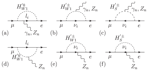
Figure 1: The leading contributions for $\mu\rightarrow e\gamma$ and $\mu-e$ conversion in the case described in SEC.III.1. The labels $n\geq 0$ indicate the KK level.

Now, briefly discuss the gauge fixing in this model. Because the orbifold parity for $\phi_{3}^{\prime}$ is chosen to be $(+-)$, it can not develop a VEV and doesn’t participate the electroweak breaking. The Goldstone bosons consist of the $y$-components of gauge bosons and the proper linear combinations of $\phi_{3}$ and $\phi_{6}$. And the whole ${\mathbf{3}}^{\prime}$, $H_{W1}^{{}^{\prime}0},H_{W1}^{{}^{\prime}\pm}$ and $H_{S}^{\prime}$ are physical Higgs. So now it is straightforward to carry out loop calculation. For further details, see Appendix.

The $E1,M1$ form factors are calculated to be:

$$f_{M1}^{Ll} = {m_{\mu}^{2}\over 384\pi^{2}M_{S0}^{2}}\sum_{i}\left[f_{Li}+{\epsilon\over 24}(9f_{Ri}+7f_{Li})\right]$$ (30)

$$f_{E1}^{Ll} = {m_{\mu}^{2}\over 384\pi^{2}M_{S0}^{2}}\sum_{i}\left[f_{Li}-{\epsilon\over 24}(9f_{Ri}-7f_{Li})\right]$$ (31)

where $f_{Li}=f_{Ri}^{*}\equiv f^{*}_{li}f_{iL}$, $M_{S0}$ is the zero mode mass of $H^{{}^{\prime}\pm}_{S}$, and $\epsilon=(\pi M_{S0}R)^{2}\sim{\cal O}(0.1)$. On arriving at the above expression, the contributions of all KK scalar excitation running in the loop have been summed. And if we drop the $\epsilon$-terms, the resulting branch ratio can be expressed as:

$$B(L\rightarrow l+\gamma) = {96\pi^{3}\alpha\over G_{F}^{2}m_{\mu}^{4}}\left(|f_{E1}^{Ll}|^{2}+|f_{M1}^{Ll}|^{2}\right)\sim{\alpha\over 768\pi G_{F}^{2}M^{4}_{S0}}\left|\sum_{i=e,\mu,\tau}f_{Li}\right|^{2}$$ (32)

$$= 2.75\times 10^{-6}\left({300\mbox{GeV}\over M_{S0}}\right)^{4}\left|(f^{{}^{\prime}3}_{S,le})^{*}f^{{}^{\prime}3}_{S,eL}+(f^{{}^{\prime}3}_{S,l\mu})^{*}f^{{}^{\prime}3}_{S,\mu L}+(f^{{}^{\prime}3}_{S,l\tau})^{*}f^{{}^{\prime}3}_{S,\tau L}\right|^{2}$$ (33)

Because the Yukawa couplings of triplet scalars are anti-symmetric, the $L\rightarrow l+\gamma$ processes have following forms:

$$B(\mu\rightarrow e+\gamma)=2.75\times 10^{-6}\left({300\mbox{GeV}\over M_{S0}}\right)^{4}\left|(f^{{}^{\prime}3}_{S,e\tau})^{*}f^{{}^{\prime}3}_{S,\mu\tau}\right|^{2}$$ (34)

$$B(\tau\rightarrow e+\gamma)=2.75\times 10^{-6}\left({300\mbox{GeV}\over M_{S0}}\right)^{4}\left|(f^{{}^{\prime}3}_{S,e\mu})^{*}f^{{}^{\prime}3}_{S,\mu\tau}\right|^{2}$$ (35)

$$B(\tau\rightarrow\mu+\gamma)=2.75\times 10^{-6}\left({300\mbox{GeV}\over M_{S0}}\right)^{4}\left|(f^{{}^{\prime}3}_{S,e\mu})^{*}f^{{}^{\prime}3}_{S,e\tau}\right|^{2}$$ (36)

We have taken $M_{3}^{\prime}=300$GeV as the reference point. If all of the Yukawa couplings are real and none of them vanishes, their ratios can be further simplified to:

$$B(\mu\rightarrow e+\gamma):B(\tau\rightarrow e+\gamma):B(\tau\rightarrow\mu+\gamma)={1\over|f^{{}^{\prime}3}_{S,e\mu}|^{2}}:{1\over|f^{{}^{\prime}3}_{S,e\tau}|^{2}}:{1\over|f^{{}^{\prime}3}_{S,\mu\tau}|^{2}}\,.$$ (37)

At this point one can use the data $B(\mu\rightarrow e+\gamma)<1.2\times 10^{-11}$PDG to obtain the constrain $\left|(f^{{}^{\prime}3}_{S,e\tau})^{*}f^{{}^{\prime}3}_{S,\mu\tau}\right|<2.1\times 10^{-3}$. This is consistent with the expectation from the study of neutrino mass in this as given in SU3:triumf . There it was found that the Yukawa coupling $f^{{}^{\prime}3}_{e\mu}$ has to be $\lesssim 10^{-2}$ and the $f$’s exhibit the pattern $f^{{}^{\prime}3}_{e\mu}>f^{{}^{\prime}3}_{e\tau}>f^{{}^{\prime}3}_{\mu\tau}$. Hence it reasonable $\mu\rightarrow e+\gamma$ to occur at a rate less than two orders of magnitude below current level. Indeed in the $SU(3)_{W}$ model we can link the various $L\rightarrow l\gamma$ transition branch ratios to the light neutrino mass matrix elements. Assuming that the light neutrino mass are mostly coming from the one-loop quantum correction involving the zero modes of $\phi_{3}^{\prime}$ and $\phi_{6}$, we have the prediction :

$$B(\mu\rightarrow e+\gamma):B(\tau\rightarrow e+\gamma):B(\tau\rightarrow\mu+\gamma)\sim\left({m_{\mu}\over m_{\tau}}\right)^{4}m_{13}m_{23}:m_{12}m_{23}:m_{12}m_{13}$$ (38)

where $m_{ij}$ is the $(ij)$ entry of the light neutrino mass matrix. Interestingly the model naturally accommodates an active neutrino mass matrix of the inverted hierarchy type as follows:

$$m\sim\left(\begin{array}[]{ccc}\epsilon&1&1\\ 1&\epsilon&\epsilon\\ 1&\epsilon&\epsilon^{2}\end{array}\right)$$ (39)

where $\epsilon\sim 0.1$. From the above equations, we see that $\mu\rightarrow e\gamma$ is suppressed compared to the $\tau\rightarrow l\gamma$ decays. This is a striking feature of the model.

III.2 $\mu-e$ conversion

The $\mu-e$ conversion in nuclei will be dominated by the virtual photon exchange. Compared to $\mu\rightarrow e\gamma$ it has additional contributions from the anapole terms. The corresponding photon $E0,M0$ form factors can be derived as:

$$\tilde{f}_{E0}(-k^{2}) = {m_{\mu}^{2}\over 576\pi^{2}M_{S0}^{2}}\sum_{i=e,\mu,\tau}\left[f_{Li}+{\epsilon\over 24}(3f_{Ri}+f_{Li})-{6\epsilon\over\pi^{2}}(f_{Ri}+f_{Li})\sum_{n=1}^{\infty}{G(\delta_{n},x_{i})\over(2n-1)^{2}}\right]$$ (40)

$$\tilde{f}_{M0}(-k^{2}) = {m_{\mu}^{2}\over 576\pi^{2}M_{S0}^{2}}\sum_{i=e,\mu,\tau}\left[f_{Li}+{\epsilon\over 24}(3f_{Ri}-f_{Li})-{6\epsilon\over\pi^{2}}(f_{Ri}-f_{Li})\sum_{n=1}^{\infty}{G(\delta_{n},x_{i})\over(2n-1)^{2}}\right]$$ (41)

where $\delta_{n}=(-k^{2})/M^{2}_{Hn}$, $x_{i}=m_{i}^{2}/(-k^{2})$, $i=e,\mu,\tau$, and

$$G(\delta,x)=-\ln\delta-\ln x+\frac{1}{3}-4x+(1-2x)\sqrt{1+4x}\ln{\sqrt{4x+1}-1\over\sqrt{4x+1}+1}.$$ (42)

As expected, the principal contribution is from the Fig.1(c) with the $H^{{}^{\prime}\pm}_{S}$ zero mode running in the loop. The logarithmic enhancements in $G(\delta,x)$, is due to the exchange of neutral scalars, $H_{W1}^{{}^{\prime}0}$ ( see Fig.1(a)). Although they are suppressed by the KK masses we find them to be compatible to the charged singlet contribution.

In this process $-k^{2}\sim m_{\mu}^{2}$ and $G$ has the following limits

$$G_{e,n}\sim-\ln\frac{m^{2}_{\mu}}{M^{2}_{Hn}}+\frac{1}{3},\;G_{\mu,n}\sim-\ln\frac{m^{2}_{\mu}}{M^{2}_{Hn}}-1.515,\;G_{\tau,n}\sim-\ln\frac{m^{2}_{\mu}}{M^{2}_{Hn}}-6.978$$ (43)

The KK sum of these logarithmic enhancements are finite:

$$\sum_{n=1}^{\infty}{1\over(2n-1)^{2}}\ln\frac{m^{2}_{\mu}}{M^{2}_{Hn}}=\frac{\pi^{2}}{8}\ln(m_{\mu}R)^{2}-0.8362$$ (44)

So the desired anapole form factors can be expressed as

$$\tilde{f}_{E0}(m_{\mu}^{2}) = {m_{\mu}^{2}\over 576\pi^{2}M_{S0}^{2}}\sum_{i=e,\mu,\tau}\left[f_{Li}+{\epsilon\over 24}(3f_{Ri}+f_{Li})+{3\epsilon\over 4}(f_{Ri}+f_{Li})[\ln(m_{\mu}R)^{2}+\eta_{i}]\right]$$ (45)

$$\tilde{f}_{M0}(m_{\mu}^{2}) = {m_{\mu}^{2}\over 576\pi^{2}M_{S0}^{2}}\sum_{i=e,\mu,\tau}\left[f_{Li}-{\epsilon\over 24}(3f_{Ri}-f_{Li})+{3\epsilon\over 4}(f_{Ri}-f_{Li})[\ln(m_{\mu}R)^{2}+\eta_{i}]\right]$$ (46)

$\{\eta_{e},\eta_{\mu},\eta_{\tau}\}=\{-1.011,0.837,6.300\}$. Again, since $f_{S}^{{}^{\prime}3}$ is anti-symmetric, only $f_{L\tau}=f^{*}_{R\tau}$ can contributes. For simplicity we assume there is no new CP violation in the scalar sector; then $f_{L}=f_{R}$ and the $\mu-e$ conversion rate in ${}^{48}_{22}Ti$ can be expressed as:

$$B^{\gamma}_{\rm conv}\sim 0.01B(\mu\rightarrow e+\gamma)$$ (47)

if taking $1/R=2$TeV and $M_{S}=300$GeV as a reference point. It is also possible to have extra contributions from KK photon and KK $Z$ excitation, Fig.1(a-f). One will need to take care of the KK number conservation in the scalar-scalar-gauge boson vertices and sum over all the possible combinations. But generally speaking, their contributions are further suppressed by $(m_{\mu}R)^{2}<2\times 10^{-9}$ compared to the photon zero mode and can be safely ignored.

The relation of Eq.(47) is based on the assumption that $f_{6}\gg f_{3}$ and $\phi_{3}^{\prime}$ is the dominate LFV source. However, we should point out that if $f_{3}$ is not so small the neutral scalar zero modes can make $\mu\rightarrow e\gamma$ and $B^{\gamma}_{\rm conv}$ compatible and deviates a lot from the pure photonic dipole prediction, Eq.(23).

Again, this demonstrates that $L\rightarrow l\gamma$ and $\mu-e$ conversion are very important for us to understand the Yukawa structure in the $SU(3)_{W}$ model.

The question now arises about the photonic dipole and anapole contribution to $\mu\rightarrow 3e$. The answer lies in Eqs.(30,31,40, 41). We estimated that

$$B(\mu\rightarrow 3e)<0.04B(\mu\rightarrow e\gamma).$$ (48)

This prediction is not very sensitive to what the Yukawa pattern is. Moreover, the decays $L\rightarrow 3l$ have overwhelming contribution from other sources of new physics in the model to which we shall turn our attention to next.

III.3 $L\rightarrow 3l$

A characteristic of the model is the existence of double charged gauge bosons with LFV couplings. This will induce $\mu\rightarrow 3e$ like processes for the $\tau$. In addition there are also KK scalars $H_{T}$ and $H_{0}$ which has LFV Yukawa couplings which are largely unknown. The Feynman diagrams for the $L\rightarrow 3l$ decays are depicted in Fig.2.

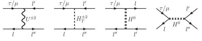
Figure 2: Feynman diagrams which lead to $\tau(\mu)\rightarrow 3l$ processes.

Since the Yukawa coupling are totally unknown, we will postpone the discussion of the contributions from scalars and look at the branch ratios, normalized to $B(\tau\rightarrow e\nu_{\tau}\bar{\nu}_{e})$, mediated by $U^{\pm 2}$ gauge boson alone first:

$$B(\tau\rightarrow 3\mu) = {\cal F}\times\left(|{\cal U}_{\tau\mu}|^{2}+|{\cal U}_{\mu\tau}|^{2}\right)|{\cal U}_{\mu\mu}|^{2}\,,$$ (49)

$$B(\tau\rightarrow 3e) = {\cal F}\times\left(|{\cal U}_{\tau e}|^{2}+|{\cal U}_{e\tau}|^{2}\right)|{\cal U}_{ee}|^{2}\,,$$ (50)

$$B(\tau\rightarrow\bar{\mu}ee) = {\cal F}\times\left(|{\cal U}_{\tau\mu}|^{2}+|{\cal U}_{\mu\tau}|^{2}\right)|{\cal U}_{ee}|^{2}\,,$$ (51)

$$B(\tau\rightarrow\mu\mu\bar{e}) = {\cal F}\times\left(|{\cal U}_{\tau e}|^{2}+|{\cal U}_{e\tau}|^{2}\right)|{\cal U}_{\mu\mu}|^{2}\,,$$ (52)

$$B(\tau\rightarrow\mu e\bar{e}) = \frac{\cal F}{8}\left(|{\cal U}_{\tau e}|^{2}+|{\cal U}_{e\tau}|^{2}\right)\times\left(|{\cal U}_{e\mu}|^{2}+|{\cal U}_{\mu e}|^{2}\right)\,,$$ (53)

$$B(\tau\rightarrow e\mu\bar{\mu}) = \frac{\cal F}{8}\left(|{\cal U}_{\tau\mu}|^{2}+|{\cal U}_{\mu\tau}|^{2}\right)\times\left(|{\cal U}_{e\mu}|^{2}+|{\cal U}_{\mu e}|^{2}\right)\,.$$ (54)

where ${\cal F}=(M_{W}\pi R)^{4}/16=1.56\times 10^{-5}(2\mbox{TeV}/1/R)^{4}$. From the analysis given in sec.II, we know all scalar operators give positive contribution. So even though we know nothing about the Yukawa couplings, we can still derive an interesting lower bond from the unitarity of ${\cal U}_{lep}$

$$B(\tau\rightarrow 3e)\geq{\cal F}\times|{\cal U}_{ee}|^{2}\left(1-|{\cal U}_{ee}|^{2}\right)\,$$ (55)

for a given $1/R$.

If one wants to keep compactification scale $1/R$ low, say $\sim 1.5$ TeV, then we would require $|{\cal U}_{ee}|$ to be either close to zero or one. Furthermore, if we take the upper bound of $1/R<5$ TeV derived from unification seriously we obtain

$$B(\tau\rightarrow 3e)>8.0\times 10^{-7}|{\cal U}_{ee}|^{2}\left(1-|{\cal U}_{ee}|^{2}\right)\,.$$ (56)

On the other hand, if we assume that the bilepton gauge boson exchange is the dominating FCNC source, another interesting upper bond can be derived:

$$B(\tau\rightarrow 3e)<\frac{\cal F}{4}=3.9\times 10^{-6}\left({2\mbox{TeV}\over 1/R}\right)^{4}$$ (57)

with $|{\cal U}_{ee}|=1/\sqrt{2}$ in Eq.(55). Actually, if all the LFV Yukawa couplings are associated with $\phi_{3}^{\prime}$ as discussed in the previous two subsections, the tree-level bilepton scalar contributions to $\tau\rightarrow 3e$ vanish due to the antisymmetry of the Yukawa couplings. However, the present experimental limit, $1-3\times 10^{-7}$ Aubert:2003pc will indicate that the compactification radius is closer to the upper limit of $5{\mathrm{T}eV}^{-1}$ for this particular case.

IV 5D $SU(5)$ model

The orbifold $SU(3)_{W}$ model discussed above has many interesting and novel features; however, the fact that quarks and leptons have to be treated differently is an obstacle towards complete unification. It’s a natural attempt to further unify the quarks and leptons in a larger GUT group. The simplest group for that is $SU(5)$. Now all fermions are on equal footing and can be clustered into 2 $SU(5)$ representations,i.e. $\Psi_{\bar{5}}=\{d^{c},L\},\Psi_{10}=\{Q,u^{c},e^{c}\}$.

Similar to the $SU(3)_{W}$ model, the model is embedded in the background geometry of $S_{1}/Z_{2}\times Z_{2}^{\prime}$ orbifold. The bulk $SU(5)$ gauge symmetry is broken to the SM by orbifold parities , with parity matrices $diag\{+++++\}$ and $diag\{---++\}$ for $Z_{2}$ and $Z_{2}^{\prime}$ transformations respectively. These are generalizations of the $SU(3)_{W}$ case.

Since no right-handed neutrinos are added, neutrino masses can be generated through quantum correction by using either $\mathbf{10}$ or $\mathbf{15}$ bulk scalars plus the $\mathbf{\overline{5^{\prime}}(10/15)\bar{5}}$ interaction mandated by breaking to the SM gauge group. The orbifold parities of $\mathbf{10}$ or $\mathbf{15}$ bulk scalars are determined to be $(++)$ by considerations of proton decay. They split into following components:

$$\mathbf{15}_{s}(++)=P_{15}\left(6,1,-\frac{2}{3}\right)_{++}+T_{15}(1,3,1)_{++}+C_{15}\left(3,2,\frac{1}{6}\right)_{+-}\,,$$

$$\mathbf{10}_{a}(++)=P_{10}\left(\bar{3},1,-\frac{2}{3}\right)_{++}+S_{10}(1,1,1)_{++}+C_{10}\left(3,2,\frac{1}{6}\right)_{+-}\,.$$

A careful analysis shows that by using $\mathbf{15(10)}$ the resultant neutrino mass matrix favor the normal(inverted) hierarchy SU5:triumf . It was also found that extra fine tuning efforts were needed to obtain phenomenologically acceptable neutrino mass patterns by using $\mathbf{10}$ alone; so we will only discuss the case which implements $\mathbf{15}$.

The $P$ components induce tree-level $K^{0}-\bar{K}^{0}$ mixing. To satisfy the experimental constraints, it is required that $M_{P}>10^{5}$ GeV. On the other hand, the two bulk Higgs in $\mathbf{5,5^{\prime}}$ which are responsible for the SM electroweak symmetry breaking share the same $(++)$ parities as $\mathbf{15}$. The brane Yukawa interaction term is easily constructed to be

$${\cal L}_{Y}=\delta(y)\left[{\tilde{f}^{15}_{ij}\over\sqrt{M^{*}/2}}\overline{\psi^{\{A\}\mathbf{c}}_{\bar{5}i}}\psi^{\{B\}}_{\bar{5}j}\phi^{\{AB\}}_{15}+H.c.\right],$$ (58)

where $A,B$ are the $SU(5)$ symmetry indices. It can be seen that to contain the necessary LFV source to generate neutrino Majorana masses.The neutrino mass matrix elements are proportional to $({\cal M})^{\nu}_{ij}\propto\sum_{k}m_{k}f^{{}^{\prime}5}_{ik}f^{15}_{jk}$ where $i,j,k$ are the generation indices and $m_{k}$ is the mass of $k$-charged lepton running in the loop.

The extra Higgs doublet in the $\mathbf{5^{\prime}}$ is good for gauge unification. By adding additional decaplet bulk fermion pair with $(+-)$ parity and mass around $10-120$ TeV, the unification is achieved at $3\times 10^{16}-10^{15}$ GeV or equivalently $1/R\sim 10^{14}$ GeV. The high scale unification or tiny radius of extra dimension makes KK excitation decouple from most phenomenological studies and basically we only need to consider the zero modes.

Below unification scale or equivalently the low energy 4D effective theory is a two Higgs doublets like model. In general the two Yukawa patterns are not aligned which that can lead to severe tree level charged neutral flavor changing (FCNC) interaction. A $Z_{2}$ symmetry is usually assumed to forbid such tree level FCNC WG . In this model, there is no such freedom since the Yukawa patterns are determined by the geometrical setup. The $\Psi_{10}$ of the first two generations are assigned to be bulk fields and the other fermion fields, $\Psi^{3}_{10}$ and $\Psi^{1,2,3}_{\bar{5}}$, are localized at the $y=0$ brane. In doing so, the salient $SU(5)$ prediction of $m_{b}/m_{\tau}$ ratio is preserved and give small hierarchy patterns in the Yukawa couplings of both $\mathbf{5,5^{\prime}}$ scalars, i.e.

$$y_{d}\propto\left(\begin{array}[]{ccc}\delta&\delta&1\\ \delta&\delta&1\\ \delta&\delta&1\end{array}\right),y_{u}\propto\left(\begin{array}[]{ccc}\delta^{2}&\delta^{2}&\delta\\ \delta^{2}&\delta^{2}&\delta\\ \delta&\delta&1\end{array}\right).$$ (65)

Due to volume dilution factor we get $\delta\sim 0.1$ which measures the amount of overlap between brane and bulk fields. The specific Yukawa pattern above successfully generates mass and mixing hierarchy of charged fermions:

$$m_{b}:m_{s}:m_{d}=m_{\tau}:m_{\mu}:m_{e}\sim 1:\delta:\delta^{2}$$ (66)

$$m_{t}:m_{c}:m_{u}\sim 1:\delta^{2}:\delta^{4}\,,\,(V_{us},V_{cb},V_{ub})\sim(\delta,\delta,\delta^{2})$$ (67)

The rotation from weak to mass eigenbasis simultaneously diagonalizes the two Higgs doublets Yukawa couplings. Thus, we do not have the FCNC problem due to mixing between two Higgs doublets.

Instead, now tree level LFV processes can be mediated by the triplet component $T_{15}$ in $\mathbf{15}$. The only important ones are the $\mu\rightarrow 3e$ like processes, see Fig.3.

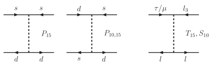
Figure 3: Feynman diagrams for tree level $K^{0}-\bar{K}^{0}$ mixing and $\mu\rightarrow 3e$ process.

An explicit calculation give the branching ratio of $\mu\rightarrow 3e$:

$$Br(\mu\rightarrow 3e)={2|f^{15{\dagger}}_{11}f^{15}_{12}|^{2}\over g_{2}^{4}(\pi RM^{*})^{2}}\left({M_{W}\over M_{T}}\right)^{4}.$$ (68)

The mass difference $\triangle M_{K}^{P}$ in $K^{0}-\overline{K^{0}}$ mixing arises from $P_{10,15}$ can be used to eliminate the ambiguity of absolute strength of Yukawa couplings. The ratio of Yukawa couplings can be replaced by the ratio of the corresponding elements in $\cal{M}_{\nu}$. Since only the $\mathbf{15}$ Higgs is used , we have

$$Br(\mu\rightarrow 3e)\sim 3.02\times 10^{-16}\left({\triangle m^{P}_{K}\over\triangle m_{K}}\right)^{2}\left(\frac{M_{P}}{M_{T}}\right)^{4}\times\left({2m_{11}m_{12}\over m_{11}m_{22}+(2\frac{m_{e}}{m_{\mu}}m_{12})^{2}}\right)^{2}.$$ (69)

It is straightforward to extend the analysis to $\tau\rightarrow 3l$ transitions. Assuming that the hierarchy of the elements of neutrino mass matrix is smaller than factor 100, this model predicts

$$Br(\mu\rightarrow 3e):Br(\tau\rightarrow 3e):Br(\tau\rightarrow 3\mu):Br(\tau\rightarrow\mu ee):Br(\tau\rightarrow e\mu\mu)$$

$$\sim\frac{m_{12}^{2}}{m_{22}^{2}}:\left(\frac{m_{\mu}}{m_{\tau}}\right)^{4}\frac{m_{13}^{2}}{m_{22}^{2}}:\left(\frac{m_{e}}{m_{\tau}}\right)^{4}\frac{m_{23}^{2}}{m_{11}^{2}}:\left(\frac{m_{\mu}}{m_{\tau}}\right)^{4}\frac{m_{23}^{2}}{m_{22}^{2}}:\left(\frac{m_{e}}{m_{\mu}}\right)^{4}\frac{m_{12}^{2}}{m_{11}m_{22}}.$$ (70)

The photonic form factors due to $T^{\pm 2},T^{\pm}$ scalar one loop diagrams can be obtained:

$$f_{M1}^{\mu e}=f_{E1}^{\mu e} = -{m_{\mu}^{2}\over 16\pi^{2}M_{T}^{2}}{5f^{15}_{i\mu}(f^{15}_{ie})^{*}\over 24}$$ (71)

$$\tilde{f}^{\mu e}_{M0}=\tilde{f}^{\mu e}_{E0} = {m_{\mu}^{2}\over 16\pi^{2}M_{T}^{2}}{f^{15}_{i\mu}(f^{15}_{ie})^{*}\over 6}\left[G(\delta,x_{i})-\frac{1}{2}\right]$$ (72)

The chiral structure in the above result is easily understood because that only the lepton doublets interact with triplet scalar.

Due to the factor $(m_{\mu}/M_{T})^{4}$, the $\mu\rightarrow e\gamma$ process is strongly suppressed. Taking $M_{T}=10^{5}$GeV, the $\mu Ti\rightarrow eTi$ conversion rate is estimated to be $\sim 1.2\times 10^{-14}|f^{15}_{i\mu}(f^{15}_{ie})^{*}|^{2}$ where we have kept only logarithmic terms which is sufficient for an order of magnitude estimate. The experimental bound is $3.6\times 10^{-11}$ PDG which is not stringent. On the other hand the recently proposed experiment aimed at a detecting a signal at the $10^{-16}-10^{-17}$ will be very encouraging. Even a negative result will provide stringent constrain on the otherwise unknown Yukawa couplings.

V Split Fermion Model

An interesting scenario was introduced by AS to solve the charged fermion masses hierarchy problem. The basic idea is to postulate that fermions are bulk fields and they interact with a non-dynamic background scalar potential. In the 5D version the bulk fermions are vectorlike, but only one of the chiral zero modes will be localized at the zero of the background potential modulated by the 5D mass terms. The chirality of the zero mode is determined by the sign of slope of the background potential at the zero point. The fermion zero modes are given a Gaussian profile in the fifth dimension and each has its own unique position in the extra dimension. The widths are controlled by the potential slope at the localized position. For simplicity, we will assume a universal width for all the SM fermions. The 5D fermion excitation are vectorlike and will be located at the same position of their zero modes. Roughly speaking, the energy gap is $\sim 1/(\mbox{Width})\gg 1/R\gg M_{W}$ and they decouple from the phenomenology we are interested in. Since the SM fermions are scattered over the fifth dimension, to preserve the gauge interaction universality the SM gauge fields are forced to be bulk fields too. To illustrate the basic physics involved it suffices to build a model on an $S_{1}/Z_{2}$ orbifold so that one can remove the unwanted $y$-components of gauge bosons zero modes which are identified with the SM gauge bosons. However, to break electroweak symmetry, a dynamic bulk Higgs is necessary.

To be more concrete we take the extra dimension to be the interval $y\in[-\pi R,\pi R]$ and the fermions are fixed in different positions $z_{i}$ in this interval. The usual Kaluza-Klein ansatz is invoked that any bulk field factorizes into a 4D field times a 5D wave function. Thus, for the fermion field we have $\psi_{i}(x,y)=g(z_{i},y)\psi(x)$ where $g(z_{i},y)$ is taken to be Gaussian distribution in the fifth dimension:

$$g(z_{i},y)={1\over(\pi\sigma_{G}^{2})^{1/4}}\exp\left[-{(y-z_{i})^{2}\over 2\sigma_{G}^{2}}\right]$$

where $\sigma_{G}$ is the universal width of Gaussian distribution. If $\sigma_{G}\ll R$, $g$ acts like the Dirac delta function. effective 4D interactions are obtained by integrating out the $y$ direction. Then any pair fermions get an exponential suppression

$$g(z_{1},y)g(z_{2},y)=\exp\left[-{(z_{1}-z_{2})^{2}\over 4\sigma_{G}^{2}}\right]g\left(\frac{z_{1}+z_{2}}{2},y\right)$$

as a result of integrating over Gaussian functions. Therefore, the linear displacement between left-handed and right-handed fermions in the fifth dimension translates into exponential Yukawa hierarchy in 4D theory. One set of solution for the quarks positions have been found numerically that can accommodate the mass hierarchy and the CKM mixingMirabelli:1999ks . To accommodate the CP violation, the overall Yukawa coupling strength of up and down type quarks must be differentBranco:2000rb ; Chang:2002ww . Although a fundamental theory of where to place the fermions are located is lacking, we have at least one realistic solution for where the quarks are located in the extra dimension. For the lepton sector, we don’t have enough constraints to pin down the solution. As pointed out byChang:2002ne ; Chang:2002ww , the FCNC interaction is induced geometrically where phenomenological constraint in quark sector have also been discussed. In fact, flavor violation is generic in any multi-position models. This comes from the fact that weak to mass eigenbasis rotations can only make the SM interactions (zero modes) flavor diagonal. the KK modes cannot be simultaneously diagonalized.

In general, the LFV can be discussed independently of the neutrino sector. The 4D effective LFV lagrangian can be expressed as

$${\cal L}^{LFV} = \sum_{n}\left({\kappa_{n}g_{2}\over\cos\theta}\right)\bar{l}_{i}\gamma^{\mu}\left[g_{L}U^{L}_{n(ij)}\hat{L}+g_{R}U^{R}_{n(ij)}\hat{R}\right]l_{j}Z_{\mu}^{n}$$ (73)

$$- \sum_{n}(\kappa_{n}e)\bar{l}_{i}\gamma^{\mu}\left[U^{L}_{n(ij)}\hat{L}+U^{R}_{n(ij)}\hat{R}\right]l_{j}A_{\mu}^{n}$$

$$+ \sum_{n}\left({\kappa_{n}g_{2}\over\sqrt{2}}\right)\bar{l}_{i}\gamma^{\mu}U^{L}_{n(ij)}\hat{L}\nu_{j}W_{\mu}^{n-}+h.c.$$

where $A^{n},Z^{n}$ and $W^{n}$ are the n-th KK excitation of the photon, $Z$ and $W$ bosons and $g_{L/R}=T_{3}(l)-Q_{l}\sin^{2}\theta_{W}$. The matrices $U^{L/R}_{n}$ are a combination of the unitary transformations $V_{L/R}$ that take the lepton weak eigenstates to their mass eigenstates and the cosine weighting of the n-th KK modes. Explicitly, they are

$$U^{L/R}_{n}=V_{L/R}^{\dagger}\mbox{diag}\left(\cos\frac{ny_{1}^{L/R}}{R},\cos\frac{ny_{2}^{L/R}}{R},\cos\frac{ny_{3}^{L/R}}{R}\right)V_{L/R}$$ (74)

for $n=0$ all the cosine factors become one and the interactions reduce to SM as expected. It is clear that the $U^{L/R}$ is no more diagonal nor unitary in general.

In this model, the $\tau\rightarrow 3l$ decay and $\mu-e$ conversion happen at tree-level, see Fig.4.

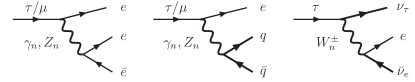
Figure 4: Flavor changing due to KK gauge bosons.

The corresponding effective LFV couplings are:

$$g_{3} = (2M_{W}R)^{2}(\sin^{2}\theta_{W}+g_{R}^{2}/\cos^{2}\theta_{W})\sum_{n=1}{U^{R*}_{n,ei}U^{R}_{n,i\mu}\over n^{2}}$$ (75)

$$g_{4} = (2M_{W}R)^{2}(\sin^{2}\theta_{W}+g_{L}^{2}/\cos^{2}\theta_{W})\sum_{n=1}{U^{L*}_{n,ei}U^{L}_{n,i\mu}\over n^{2}}$$ (76)

$$g_{5} = (2M_{W}R)^{2}(\sin^{2}\theta_{W}+g_{R}g_{L}/\cos^{2}\theta_{W})\sum_{n=1}{U^{R*}_{n,ei}U^{L}_{n,i\mu}\over n^{2}}$$ (77)

$$g_{6} = (2M_{W}R)^{2}(\sin^{2}\theta_{W}+g_{L}g_{R}/\cos^{2}\theta_{W})\sum_{n=1}{U^{L*}_{n,ei}U^{R}_{n,i\mu}\over n^{2}}$$ (78)

and the $v,a,v_{q}$ and $a_{q}$ can be obtained in a similar way. Also the lepton universality is broken due to flavor dependent couplings in the KK gauge interaction. We refer the reader to Chang:2002ne for a detailed analysis.

The leading $\mu\rightarrow e\gamma$ contribution comes from the one loop corrections. We need to fix the gauge before proceeding. The necessary details of 5D gauge fixing are collected in the appendix. After properly identifying the Goldstone boson, the usual 4D $R_{\xi}$ gauge technique can be straightforwardly applied here. Note that the Yukawa couplings of the physical KK scalars are suppressed by the factor of $\sim(m_{l}R)/n$. Although there is residual GIM cancellation in the KK gauge boson interaction, we expect the leading LFV are from KK gauge interaction.

The LFV photonic form factors due to KK gauge boson and their Goldstone boson can be calculated. The KK $W$ bosons’ contribution to the photonic form factors are given by:

$$f^{W}_{M1} = f^{W}_{E1}={7\over 24}{g_{2}^{2}\over 16\pi^{2}}\sum_{n=1}{(m_{\mu}R)^{2}\over n^{2}}U^{L*}_{n,ie}U^{L}_{n,i\mu},$$ (79)

$$\widetilde{f^{W}_{M0}} = \widetilde{f^{W}_{E0}}={23\over 72}{g_{2}^{2}\over 16\pi^{2}}\sum_{n=1}{(m_{\mu}R)^{2}\over n^{2}}U^{L*}_{n,ie}U^{L}_{n,i\mu}$$ (80)

and for the KK $Z$ bosons they are

$$f^{Z}_{M1/E1} = {(m_{\mu}R)^{2}\over 8\pi^{2}}{g_{2}^{2}\over\cos^{2}\theta}\sum_{n=1}\sum_{i}{1\over n^{2}}\left\{-\frac{1}{3}\left[g_{L}^{2}U^{L*}_{n,ie}U^{L}_{n,i\mu}\pm g_{R}^{2}U^{R*}_{n,ie}U^{R}_{n,i\mu}\right]\right.$$ (81)

$$\left.+\frac{m_{i}}{m_{\mu}}g_{L}g_{R}\left[U^{L*}_{n,ie}U^{R}_{n,i\mu}\pm U^{R*}_{n,ie}U^{L}_{n,i\mu}\right]\right\},$$

$$\widetilde{f^{W}}_{E0/M0} = -{(m_{\mu}R)^{2}\over 24\pi^{2}}{g_{2}^{2}\over\cos^{2}\theta}\sum_{n=1}\sum_{i}{1\over n^{2}}\left\{\left(G(\delta_{n},x_{i})+\frac{1}{2}\right)\left[g_{L}^{2}U^{L*}_{n,ie}U^{L}_{n,i\mu}\pm g_{R}^{2}U^{R*}_{n,ie}U^{R}_{n,i\mu}\right]\right\}$$ (82)

Similar contributions from KK photons can be easily read from the above by replacing $(g_{2}/\cos\theta)\rightarrow e$, $g_{L}\rightarrow 1$, and $g_{R}\rightarrow 1$.

These photonic form factors give extra contribution to $\mu\rightarrow 3e$ and $\mu-e$ conversion processes but can’t compete with those tree-level KK gauge boson exchanging diagrams. However they are the sole sources of new physics for the $L\rightarrow l+\gamma$ process.

In addition to the usual ignorance with regard to Yukawa coupling there are more unknowns in the lepton locations and the Gaussian widths. Ad hoc simplifying assumptions have to be made. Hence, this kind of model suffers from a lack of predictive power in LFV studies. More data such as the scale of neutrino mass and more complete knowledge of the neutrino mixing matrix will help greatly. However, we can extract some generic features for this kind of models as follow:

1. $\mu/\tau\rightarrow 3l$ and $\mu Ti\rightarrow eTi$(or $\tau\rightarrow l+{\mathrm{hadrons}}$) will happen at tree-level from the exchange of KK scalars, photons and $Z$ bosons.

2. $L\rightarrow l\gamma$ proceeds at the one-loop level and hence is expected to be suppressed compared to the previous modes

3. Violation of lepton universality will occur. The best signal will be to look for the violation in $W\rightarrow l_{i}\nu_{i}$ decays Chang:2002ne .

Unfortunately a more quantitative statement about the level of the effect eludes us for now.

VI Conclusion

We have studied and reviewed LFV processes in 5D gauge models that are related to neutrino mass generation or address the flavor problem. Specifically we focus on two complete models which generate neutrino masses radiatively. This allows us to see in detail how the two issues can be related. The models are based on $SU(3)_{W}$ and $SU(5)$ 5D unification. They give rise to different neutrino mass patterns SU3:triumf ; SU5:triumf ; thus, it is not surprising that they give different prediction for LFV. The $SU(3)_{W}$ model has a unification scale at $\sim{\mathrm{T}eV}$ and makes essential use of bileptonic scalars. It also contains characteristic doubly charged gauge bosons. The $SU(5)$ model is a 5D orbifold version of the usual GUT. The unification scale is much higher at $10^{15}$ GeV. The important ingredient for LFV and neutrino masses is the $\mathbf{1}5$ Higgs representation. The triplet Higgs of this model plays the crucial role here.

We found that for the $SU(3)_{W}$ model the rare $\tau$ decays are much more enhanced compare to their counterpart $\mu$ decays. Among the $\tau\rightarrow l+\gamma$ decays the largest mode is the $\mu+\gamma$. Even for this mode we expect it to be $<10^{-14}$ which is much lower then current experimental reach.

The decay modes $\tau\rightarrow 3l$ have a better chance of being observe. This stems from the fact that they are tree level processes induced by the bileptonic gauge bosons or scalars. Since they are KK modes they have high masses controlled by the extra dimension compactification radius which is $\leq 5{\mathrm{T}eV}$ from consistency and unification considerations. An order of magnitude improvement on the current limit will be valuable information on the unknown Yukawa couplings.

For the orbifold 5D $SU(5)$ model the muon to electron conversion in nuclei can be within the experimental capability of the proposed experiment at Brookhaven National LaboratoryPopp:2001hu . As in the previous model $\mu\rightarrow e+\gamma$ will not be observable. This is very different conventional 4D unificational models.

The split fermion model also have the characteristic of $L\rightarrow 3l$ and $\mu\rightarrow e$ conversion dominating over $L\rightarrow l\gamma$. We cannot be more quantitative due to proliferation of unknown parameters. This model have lepton universality violation which is not present in the previous two models. This can serve as a differentiating tool.

It is clear that in order to unravel the physics behind the flavor problem all modes of LFV must be searched for. The usual 4D supersymmetric model will favor $L\rightarrow l\gamma$ where as the 5D models prefer $L\rightarrow 3l$ and/or $\mu\rightarrow e$ conversion. To this we add lepton universality test as a probe.

Appendix A $SU(2)\times U(1)$ in 5D $S_{1}/Z_{2}$ model with a brane at $y=0$

Now we present the gauge fixing scheme used for the 5D electroweak interaction with one bulk Higgs doublet. For simplicity the background geometry is $S_{1}/Z_{2}$. The fifth gamma matrix was chosen to be $\gamma^{y}=i\gamma^{5}$. The 5D Lagrangian is

$${\cal L}_{5} = -\frac{1}{4}F^{MN}F_{MN}-\frac{1}{4}G^{(a),MN}G^{(a)}_{MN}+\left(D_{M}\Phi\right)^{\dagger}\left(D^{M}\Phi\right)+\cdots$$ (83)

where

$$F_{MN} = \partial_{M}B_{N}-\partial_{N}B_{M}\,,$$

$$G^{(a)}_{MN} = \partial_{M}A^{(a)}_{N}-\partial_{N}A^{(a)}_{M}+{\tilde{g}_{2}\over\sqrt{M^{*}}}\epsilon^{abc}A_{M}^{(b)}A_{N}^{(c)}\,$$

$$D_{M} = \partial_{M}-i{\tilde{g}_{2}\over\sqrt{M^{*}}}\frac{\tau^{(a)}}{2}A_{M}^{(a)}.-i{\tilde{g}_{1}Y\over\sqrt{M^{*}}}B_{M}$$

$B$ and $A$ stand for the $U(1)$ hyper charge and $SU(2)$ gauge fields respectively. In this convention, $Q=T_{3}+Y$. We adopt the usual conventions: $W^{M}_{\pm}=\frac{1}{\sqrt{2}}(A_{1}^{M}\mp iA_{2}^{M})$, $P^{M}(\mbox{hoton})=(c_{W}B^{M}+s_{W}A_{3}^{M})$ and $Z^{M}=(c_{W}A_{3}^{M}-s_{W}B^{M})$, or $B^{M}=c_{W}P^{M}-s_{W}Z^{M},A_{3}^{M}=c_{W}Z^{M}+s_{W}P^{M}$), where $c_{W}=\tilde{g}_{2}/\sqrt{\tilde{g}_{1}^{2}+\tilde{g}_{2}^{2}}$ and $s_{W}=\tilde{g}_{1}/\sqrt{\tilde{g}_{1}^{2}+\tilde{g}_{2}^{2}}$. $\tilde{g}_{5}=\sqrt{\tilde{g}_{1}^{2}+\tilde{g}_{2}^{2}}$ are introduced to simplify the notation. The symmetry breaking pattern is same as in the usual 4D SM. The bulk Higgs doublet acquires a nonzero VEV after SSB,

$$\Phi=\left(\begin{array}[]{c}h^{+}\\ {\tilde{v}_{b}+h^{0}\over\sqrt{2}}\end{array}\right)\,\,,\,h^{0}=\phi^{0}+i\chi^{0}\,.$$ (84)

The generalized linear $R_{\xi}$ gauge fixing is introduced GaugeFixing (other schemes can be found in GFCoV ),

$${\cal L}_{GF}= - \frac{1}{2\xi}\left(\partial_{\mu}P^{\mu}+\xi\partial_{y}P^{y}\right)^{2}$$ (85)

$$- \frac{1}{\xi}\left|\partial_{\mu}W^{+,\mu}+\xi\left[\partial_{y}W^{+,y}-iM_{W}h^{+}\right]\right|^{2}$$

$$- \frac{1}{2\xi}\left(\partial_{\mu}Z^{\mu}+\xi\left[\partial_{y}Z^{y}-M_{Z}\chi^{0}\right]\right)^{2}.$$

to remove the mixing between gauge bosons and Higgs. Therefore, the Goldstone bosons and the physical scalars can be easily identified:

$$G^{\gamma}_{n} = P^{y}_{n}\,,\,M_{\gamma}^{(n)}=n/R$$ (86)

$$G^{0}_{n} = \left[c^{Z}_{n}Z_{n}^{y}-s^{Z}_{n}\chi^{0}_{n}\right]\,,\,S^{0}_{n}=\left[s^{Z}_{n}Z_{n}^{y}+c^{Z}_{n}\chi^{0}_{n}\right]$$ (87)

$$M_{Z}^{(n)}=\sqrt{n^{2}/R^{2}+M_{Z}^{2}}\,,\,s^{Z}_{n}=M_{Z}/M_{Z}^{(n)}$$

$$G^{\pm}_{n} = \left[c^{W}_{n}W_{n}^{y\pm}\mp is^{W}_{n}h^{\pm}_{n}\right]\,,\,H^{\pm}_{n}=\left[s^{W}_{n}W_{n}^{y\pm}\pm ic^{W}_{n}h^{\pm}_{n}\right]$$ (88)

$$M_{W}^{(n)}=\sqrt{n^{2}/R^{2}+M_{W}^{2}}\,,\,s^{Z}_{n}=M_{W}/M_{W}^{(n)}$$

$$H^{0}_{n} = \phi^{0}_{n}\,,\,M_{H}^{(n)}=\sqrt{n^{2}/R^{2}+M_{\phi}^{2}}$$ (89)

where $G^{0}$ and $G^{\pm}$ are the KK Goldstone bosons, $S^{0}$ is the physical KK pseudo scalar, and $H^{0},H^{\pm}$ are the physical KK scalars. The usual $R_{\xi}$ gauge can be extended to the 5D $S_{1}/Z_{2}$ model with little modification, like $M_{W}\Rightarrow M_{W}^{(n)}$ and so on.

The Goldstone bosons are mainly constituted by the fifth gauge components with a small fraction of KK Higgs bosons mixed interaction. On the other hand the Goldstone bosons couple to brane fermions through their Higgs components. In contrast the physical scalars are mainly composed of KK Higgs plus small amount of the fifth components of gauge fields.

This scheme can also be applied to the models built on the $S_{1}/(Z_{2}\times Z^{\prime}_{2})$ orbifold with little modification.

Appendix B Gauge fixing for the orbifold models with more than one scalars.

The method can be easily extended to the cases with multi scalars. Taking a 5D two Higgs doublets Model(2HDM) as an example, with VEVs $\langle\phi_{1}\rangle=v_{1}$, $\langle\phi_{2}\rangle=v_{2}$ and $\tan\beta=v_{2}/v_{1}$, the physical charged scalars and pseudoscalars are

$$H^{\pm}=\sin\beta\phi_{1}^{\pm}-\cos\beta\phi_{2}^{\pm}\,,\,A^{0}=\sin\beta Im\phi_{1}^{0}-\cos\beta Im\phi_{2}^{0}$$ (90)

just like the usual 4D 2HDM. The only difference is that the orthogonal linear combinations $a^{0}=\cos\beta Im\phi_{1}^{0}+\sin\beta Im\phi_{2}^{0}$ and $g^{\pm}=\cos\beta\phi_{1}^{\pm}+\sin\beta\phi_{2}^{\pm}$ will mix with the fifth components of gauge fields to form the real Goldstone bosons:

$$G^{0}_{n} = \cos\theta^{0}_{n}V^{0}_{n}-\sin\theta^{0}_{n}a^{0}_{n}\,,\,\sin\theta^{0}_{n}=M_{0}/\sqrt{M_{0}^{2}+n^{2}/R^{2}}\,,$$ (91)

$$G^{\pm}_{n} = \cos\theta^{\pm}_{n}V^{\pm}_{n}\mp i\sin\theta^{\pm}_{n}g^{\pm}_{n}\,,\,\sin\theta^{\pm}_{n}=M_{V}/\sqrt{M_{V}^{2}+n^{2}/R^{2}}\,.$$ (92)

References

(1)
Y. Fukuda et al. [Super-Kamiokande Collaboration],
Phys. Rev. Lett. 8119981562
[hep-ex/9807003].
(2)
Q. R. Ahmad et al. [SNO Collaboration],
Phys. Rev. Lett. 892002011301
[nucl-ex/0204008].
(3)
K. Eguchi et al. [KamLAND Collaboration],
Phys. Rev. Lett. 902003021802
[hep-ex/0212021].
(4)
C. L. Bennett et al.,
[astro-ph/0302207].
(5)
A. Masiero, S.K. Vempati, and O. Vives, Nucl. Phys. B 649, 189 (2003)
T. Blazek and S.F. King, ibid662, 359 (2004)
(6)
W.F. Chang and J.N. Ng [archiv:hep-ph/0411201]
(7)
C. H. Chang, W. F. Chang and J. N. Ng,
Phys. Lett. B 558, 92 (2003)
[arXiv:hep-ph/0301271].
(8)
W. F. Chang and J. N. Ng,
JHEP 0310, 036 (2003)
[arXiv:hep-ph/0308187].
(9)
J.N. Ng, J. Korean Phy. Soc. 45 S341 (2004)
(10)
Y. Kuno and Y. Okada,
Rev. Mod. Phys. 73, 151 (2001)
[arXiv:hep-ph/9909265] and references therein.
(11)
S. T. Petcov,
Phys. Lett. B 68, 365 (1977).
(12)
K. Huitu, J. Maalampi, M. Raidal and A. Santamaria,
Phys. Lett. B 430, 355 (1998)
[arXiv:hep-ph/9712249].
T. S. Kosmas, S. Kovalenko and I. Schmidt,
Phys. Lett. B 511, 203 (2001)
[arXiv:hep-ph/0102101].
(13)
G. Feinberg and S. Weinberg,
Phys. Rev. Lett. 3, 527 (1959).
(14)
R. Kitano, M. Koike and Y. Okada,
Phys. Rev. D 66, 096002 (2002)
[arXiv:hep-ph/0203110].
(15)
H. C. Chiang, E. Oset, T. S. Kosmas, A. Faessler and J. D. Vergados,
Nucl. Phys. A 559, 526 (1993).
(16)
S. Weinberg, Phys. Rev. D 2, 1962 (1975)
(17)
L.J. Hall and Y. Normura, Phys. Lett. B 532 111 (2002)
T. Li and W. Liao, ibid 545 147 (2002)
S. Dimopoulos,D.E. Kaplan, and N. Weiner, ibid534 124 (2002)
I. Antoniadis and K. Benakli, ibid326 69 (1994)
(18)
A. Zee, Phys. Lett. B 161 141 (1985)
(19)
Particle Data Group, Phys. Lett. B 592 410 (2004)
(20)
B. Aubert et al. [BABAR Collaboration],
Phys. Rev. Lett. 92 121801 (2004)
(21)
S. Glashow and S. Weinberg, phys. Rev. D 15 1958 (1977).
(22)
N. Arkani-Hamed and M. Schmaltz,
Phys. Rev. D 61, 033005 (2000)
[arXiv:hep-ph/9903417];
N. Arkani-Hamed, Y. Grossman and M. Schmaltz,
Phys. Rev. D 61, 115004 (2000)
[arXiv:hep-ph/9909411].
(23)
E. A. Mirabelli and M. Schmaltz,
Phys. Rev. D 61, 113011 (2000)
[arXiv:hep-ph/9912265].
(24)
G. C. Branco, A. de Gouvea and M. N. Rebelo,
Phys. Lett. B 506, 115 (2001)
[arXiv:hep-ph/0012289].
(25)
W. F. Chang and J. N. Ng,
JHEP 0212, 077 (2002)
[arXiv:hep-ph/0210414].
(26)
W. F. Chang, I. L. Ho and J. N. Ng,
Phys. Rev. D 66, 076004 (2002)
[arXiv:hep-ph/0203212].
(27)
J. L. Popp [MECO Collaboration],
Nucl. Instrum. Meth. A 472, 354 (2000)
[arXiv:hep-ex/0101017].
(28)
D. M. Ghilencea, S. Groot Nibbelink and H. P. Nilles,
Nucl. Phys. B 619, 385 (2001)
[arXiv:hep-th/0108184];
A. Muck, A. Pilaftsis and R. Ruckl,
Phys. Rev. D 65, 085037 (2002)
[arXiv:hep-ph/0110391].
(29)
For example,
K. R. Dienes, E. Dudas and T. Gherghetta,
Nucl. Phys. B 537, 47 (1999)
[arXiv:hep-ph/9806292];
J. Papavassiliou and A. Santamaria,
Phys. Rev. D 63, 125014 (2001)
[arXiv:hep-ph/0102019];