SCUPHY-TH-05001

SHEP-04-18

TUHEP-TH-04146

Pair-produced heavy particle topologies:

MSSM neutralino properties

at the LHC from gluino/squark cascade decays

M. Bisset, N. Kersting, J. Li

Center for High Energy Physics and Department of Physics,

Tsinghua University,

Beijing, 100084 P.R. China

F. Moortgat

PH Department, CERN, CH-1211 Geneva 23, Switzerland

S. Moretti

School of Physics and Astronomy

University of Southampton

Highfield, Southampton SO17 1BJ, UK

Q.L. Xie

Department of Physics

Sichuan University

Chengdu, 610065 P.R. China

Processes of the form $pp\to anything\to X_{i}X_{j}\to x\bar{x}+y\bar{y}\;(+\hbox to0.0pt{\hbox to7.95831pt{\hfil/\hfil}\hss}E)$ are studied via a technique that may be viewed as an adaptation of time-honoured Dalitz plot analyses. $X_{i}$ and $X_{j}$ are new heavy states (with $i,j=1...n$), which may be identical or distinct; and $x\bar{x}$ and $y\bar{y}$ are necessarily distinct Standard Model (SM) fermion pairs whose invariant masses can be measured. A Dalitz-like plot of said invariant masses, $M(x\bar{x})$ vs. $M(y\bar{y})$, exhibits a topology connected to the masses and specific decay chains of $X_{i}$ and $X_{j}$. Aside from relatively minor details, observed patterns consist of a collection of box and wedge shapes. This collection is model-dependent: comparison of the observed pattern to the possibilities for a specific model yields information on which new particle pair combinations are actually being produced, information beyond that extractable from conventional one-dimensional invariant mass distributions. The technique is illustrated via application to the Minimal Supersymmetric Standard Model (MSSM) process $pp\to\tilde{g}\tilde{g},\tilde{g}\tilde{q},\tilde{q}\tilde{q}\to\widetilde{\chi}_{i}^{0}\widetilde{\chi}_{j}^{0}\to e^{+}e^{-}\,+\,\mu^{+}\mu^{-}\;(+\hbox to0.0pt{\hbox to7.95831pt{\hfil/\hfil}\hss}E)$. Here the heavy states are neutralinos $\widetilde{\chi}_{i}^{0}$ ($i=2,3,4$) — note $\widetilde{\chi}_{1}^{0}$ is excluded — which are produced in gluino/squark ($\tilde{g}$/$\tilde{q}$) cascade decay chains. Even with fairly modest expectations for the LHC performance during the first few years, this method still provides substantial insight into the neutralino mass spectrum and couplings if gluino/squark masses are relatively low ($\simeq\,400\,\hbox{GeV}$).

Introduction

The field of particle physics is nearing a critical juncture: up to now the highly successful SM — whose predictions of various cross-sections and precision observables are in excellent agreement with data from the most advanced particle accelerators to date — has been sufficient to meet the experimental demands; however, the SM is theoretically incomplete and cannot continue to describe physics at energies much higher than $1\,\hbox{TeV}$. Most theoretical extensions of the SM designed to address this problem predict new heavy degrees of freedom at or near the TeV-scale. The soon-to-be-completed LHC, with a centre-of-mass energy of $14\,\hbox{TeV}$, should readily produce such heavy particles if they couple significantly to SM ones. Then experiment will certainly require more guidance than the SM can provide. Different extensions to the SM differ in the predicted number and types of new heavy particles. It is therefore imperative to understand what the decays of such heavy particles (at least some of which are typically unstable) would look like at a hadron collider in as model-independent a way as possible.

This work is particularly concerned with neutral heavy particles produced in pairs, $X_{i}X_{j}$, with $i,j=1...n$ — the exact value of $n$ being model dependent, but for the present work it may be any integer greater than 1 (thus $X_{i}$ and $X_{j}$ may or may not be distinct). These pairs may be produced directly as per $pp\to X_{i}X_{j}$ or as a result of cascade decays from the production of other even heavier new particles (in fact the latter production mode is dominant in the specific case examined below).

The introduction of new heavy particle states often comes with the introduction of a new conserved quantum number (or numbers) associated with a new discrete ${\cal Z}_{n}$ symmetry (or symmetries) — for example, the attractive $R$-parity  [2] conservation in numerous SUSY extensions to the SM. Another example is found in some little Higgs models in which an extra ${\cal Z}_{2}$ symmetry is introduced to tame excessive flavour-changing neutral processes  [3]. Conservation of such a new quantum number(s) typically dictates the pair production of new particle states as well as the stability of the lightest new particle which is “odd” under the new symmetry (features typically associated with $R$-parity conserving SUSY scenarios but in fact they seem to be more generally applicable).

Any sample of events collected over time may be a superposition of different $X_{i}X_{j}$ channels. The technique introduced here is ideally suited for precisely this situation. Unlike at an $e^{+}e^{-}$ collider, at a hadron collider the centre-of-mass energy of the parton-level hard scattering process cannot be controlled, and thus said parton-level centre-of-mass energy cannot be incrementally raised to scan through the different $X_{i}X_{j}$ thresholds. Rather, all such channels may be produced simultaneously and must subsequently be disentangled to the extent it is possible in the decay analysis.

The new heavy particles are assumed to decay (possibly indirectly) into pairs of SM fermions $X_{i}\to y\bar{y}$ (accompanied in some models containing stable but undetectable heavy particle states by the observation of substantial missing energy in the detector). Thus pair production and subsequent decay of the new heavy particles can result in end-states of the form $x\bar{x}\;+\;y\bar{y}$ , where $x\bar{x}$ and $y\bar{y}$ are distinct SM particle pairs whose invariant masses are measurable with sufficient precision. For example, same-flavour oppositely-charged lepton pairs $e^{+}e^{-}$ and $\mu^{+}\mu^{-}$ (utilised in the following application to the MSSM  [2]) might be chosen since these are most easily extracted from the overwhelming QCD backgrounds at a hadron collider. Other choices, such as $b\overline{b}$ or $\tau^{-}\tau^{+}$, are also possible though, and might prove more appropriate in some cases. Decays to SM gauge bosons may merit attention, though with decays to $Z^{0}$’s a $Z^{0}$-veto to reduce backgrounds is no longer possible while decays to $W$’s will require reconstruction of hadronically-decaying $W$’s. The remainder of this work concentrates on decays into pairs of fermions, and, more specifically, into electrons and muons. Use of similar ideas for the pair-production of charged states ($X_{i}^{+}X_{j}^{-}$) also might merit future investigation.

Speaking generally, the experimentally measurable quantities of interest are the fermion pair invariant masses $M(x\bar{x})$ and $M(y\bar{y})$. Other processes besides the sought-after heavy particle decays may also produce an $(x\bar{x},y\bar{y})$-topology. Thus cuts will probably be needed to purify the event sample, and a partially-contaminated sample may have to suffice. It will be shown below that, for several realistic MSSM scenarios including both signals and backgrounds, making a two-dimensional Dalitz-like  [4] plot of $M(x\bar{x})$ vs. $M(y\bar{y})$ can reveal information about the spectrum of the heavy particles produced (kinematics) as well as relative production cross sections (dynamics).

Topological Analysis

Any Dalitz-like plot of $M(x\bar{x})$ vs. $M(y\bar{y})$ resulting from heavy particle pair production will be a superposition of specific topological shapes. At the coarsest level, these shapes may be bifurcated into two types:

• Box-like — A ‘box’ in the $M(x\bar{x})$-$M(y\bar{y})$ plane results from the decay

  $$X_{i}X_{i}\to x\bar{x}+y\bar{y}\;\;(+\hbox to0.0pt{\hbox to7.95831pt{\hfil/\hfil}\hss}E)\;,$$ (1)

  since the invariant masses $M(x\bar{x})$ and $M(y\bar{y})$ are bounded from below by the masses of $x,y$ (approximately zero if $x,y$ are leptons) and above by the maximum for $M_{X_{i}}-\hbox to0.0pt{\hbox to7.95831pt{\hfil/\hfil}\hss}E$ (this is a well-defined limit if the model in question completely accounts for $\hbox to0.0pt{\hbox to7.95831pt{\hfil/\hfil}\hss}E$ by particles which do not decay in the detector).

• Wedge-like — A ‘wedge’ or ‘L-shape’ results from the decay

  $$X_{i}X_{j}\to x\bar{x}+y\bar{y}\;\;(+\hbox to0.0pt{\hbox to7.95831pt{\hfil/\hfil}\hss}E)\;\;\;\;(i\neq j)\;;$$ (2)

  i.e., if the $x\bar{x}$ came from $X_{i}$ then the $y\bar{y}$ presumably comes from $X_{j}$ — here it is assumed neither $x$- nor $y$-flavour number is violated in the heavy-particle decays. Therefore $0<M(x\bar{x})<M_{X_{i}}-\hbox to0.0pt{\hbox to7.95831pt{\hfil/\hfil}\hss}E$ and $0<M(y\bar{y})<M_{X_{j}}-\hbox to0.0pt{\hbox to7.95831pt{\hfil/\hfil}\hss}E$. On the other hand if the decays are swapped then $0<M(x\bar{x})<M_{X_{j}}-\hbox to0.0pt{\hbox to7.95831pt{\hfil/\hfil}\hss}E$ and $0<M(y\bar{y})<M_{X_{i}}-\hbox to0.0pt{\hbox to7.95831pt{\hfil/\hfil}\hss}E$; the superposition of these two strips forms the wedge.

The manner in which $X_{i}$ and $X_{j}$ decay may introduce new features on top of these two basic forms. For example, whether the decay proceeds through a series of two-body decays or via a three-body decay. Furthermore, if some $X_{i}$ involved in the decay chain has two or more ways to decay to $x\bar{x}$ and $y\bar{y}$; e.g., if two or more decay chains resulting in $X_{i}\to X_{j}+x\bar{x}(\hbox{or}~{}y\bar{y})$ are kinematically allowed for any given $i$, Dalitz-like plots will have ‘stripes’ extending from each of the endpoints of these decays to zero (or to $m_{x,y}$ if these are not approximately massless); these stripes will overlay the basic box/wedge structure outlined above.

If the types of decay chains the $X_{i}$ follow are known and in particular if one type dominates (e.g., two-body decays through one or more known intermediate states), the shape of the $x\bar{x}$($y\bar{y}$) invariant mass spectrum can be predicted and this information used to compare densities of points in different regions of the Dalitz-like plot; this in turn allows one to measure ratios of cross section $\times$ BR for the different modes $X_{i}X_{j}$ which are responsible for the various Dalitz shapes. The Dalitz-like plots can then provide information about dynamics in addition to kinematics (contained in the location of the endpoints).

In any particular model there will be a set number of heavy particles expected to be produced at LHC energies; therefore the types of possible boxes and wedges is likewise set and the number of possible box-wedge combinations (with possible overlaying stripes) is fixed. Only some of these combinations are topologically distinct. For example, consider a sample of events where two $X_{i}X_{i}$-type production modes dominate. This will yield a Dalitz-like plot that looks like a ‘box within a box’ (ignore stripes for the moment). The topology alone would not indicate whether $X_{2}X_{2}$ and $X_{3}X_{3}$ are being produced or $X_{4}X_{4}$ and $X_{5}X_{5}$ are being produced. A collection of Dalitz patterns form a topological class if they can be transformed into each other by any amount of dilation; i.e., they can be deformed into each other without crossing any kinematical hard edges. Furthermore, a wedge of type ij is difficult to distinguish from an ij-wedge and an ii-box ($M_{X_{i}}<M_{X_{j}}$) combination and thus these two cases will be treated as topologically equivalent. If stripes are present the amount of degeneracy escalates (see subsequent application to SUSY).

Application to Sparticle Decays

The $R$-parity conserving MSSM is next considered as a test-case for this technique. In the MSSM, there are four distinct neutralinos, the lightest of which, $\widetilde{\chi}_{1}^{0}$, is supposed to be stable and undetectable (e.g., in minimal supergravity-inspired models). These –inos are the physical eigenstates resulting from the two pairs of neutral electroweak (EW) gauginos and Higgsinos in the MSSM. Consider –ino pair production. More specifically, the modes of interest here are pair production of heavy –inos:

$$pp\to\hbox{intermediate(s)}\to\widetilde{\chi}_{i}^{0}\widetilde{\chi}_{j}^{0}\;\;\;\;(i,j=2,3,4),$$ (3)

where both of the –inos subsequently decay (in the detector, as expected in all MSSM scenarios) leading to final states of the type described above. Thus neither –ino is allowed to be the stable Lightest Supersymmetric Particle (LSP) $\widetilde{\chi}_{1}^{0}$. However, in each event two LSP $\widetilde{\chi}_{1}^{0}$’s are subsequently produced from the decays of the two initial heavy –inos, possibly through a chain of decays, along with the $e^{+}e^{-}$ and ${\mu}^{+}{\mu}^{-}$ pairs we demand.

Figure 1: Feynman diagrams for heavy ($i,j=2,3,4$) neutralino pair production
mechanisms: (a) ‘direct’ production via EW gauge boson; (b) Higgs-mediated production; and (c) production via cascade decays of gluinos (shown here) or via gluino/squark or squarks — to obtain these diagrams, make one or both of the squarks in $(c)$ on-mass shell and remove the associated gluino(s) and the connected quark(s).

At the LHC, heavy –ino pair production occurs via virtual SM gauge bosons (termed “direct production”), via the decays of heavy Higgs bosons, or via cascade decays of coloured squarks and gluinos (see Figure 1). The last of these, production via coloured intermediates,

$$pp\to\tilde{g}\tilde{g},\,\tilde{g}\tilde{q},\,\tilde{q}\tilde{q}\to\widetilde{\chi}_{i}^{0}\widetilde{\chi}_{j}^{0}\;\;\;\;(i,j=2,3,4),$$ (4)

will be the focus of the current work. Due to the strong coupling, (4) has the potential for yielding the largest number of signal events, if the intermediate gluinos and squarks are sufficiently light. Rates from EW direct production are typically too low for the technique described herein to be effectively utilised, except perhaps in certain minor regions of un-excluded parameter space or with allowance for ample time to gather more events  [7]. Since the lightest MSSM Higgs boson ($h^{0}$) can only yield LSP-containing –ino pairs, the Higgs-mediated production modes of interest involve the heavier MSSM Higgs bosons ($H^{0}$ and $A^{0}$). Their masses need to be in the correct range to get sufficient Higgs boson production and yet have open decay modes to exclusively-heavy –ino pairs. This is certainly possible, as will be documented in another work  [5, 7]. However, the EW production rate will lead to a smaller number of potential signal events than for (4). Thus, (4) should be the main source of –inos at the LHC if gluinos are light ($\sim 400\,\hbox{GeV}$). In the current work, inputs for gluinos and squarks will be set near the lower end of their allowed mass ranges while the input Higgs boson mass will be fixed fairly high up (${\sim}700\,\hbox{GeV}$).

Aside from the larger possible signal rates with (4) as compared to with the two EW production mechanisms, there are two other seminal distinctions between (4) and the other two that can strongly influence the analysis. First, as a side-product to producing –inos, the decaying gluinos/squarks in (4) also typically lead to jet activity in the final state, whereas the other two production mechanisms may be hadronically quiet much or at least some of the time. Thus backgrounds to (4) may be more severe / less amenable to cuts. This could bring the signal rate after cuts down to the level of the other two processes. In fact, it will be shown in the simulations section to follow that the backgrounds are not so severe. Further, demanding the presence of jets is actually useful in reducing some backgrounds.

The second point warranting attention is that in (4) the two –inos are produced separately, whereas in the two EW processes there is an –ino–ino^(′)-$S$ vertex (where $S$ is a SM gauge boson or an MSSM heavy Higgs boson). If the cascade decays were solely from $\tilde{g}\tilde{g}$ and/or $\tilde{q}\tilde{q}$ production, where here both squarks are of the same flavor and had the same $SU(2)_{\hbox{\smash{\lower 0.75346pt\hbox{${\scriptstyle L}$}}}}$ quantum number (e.g., $\widetilde{u}_{L}\widetilde{u}_{L}^{*}$ $\widetilde{d}_{R}\widetilde{d}_{R}^{*}$, etc.), this would reduce the number of possible topologies that can result from (4) relative to the other production mechanisms (that is, considering $\widetilde{\chi}_{i}^{0}\widetilde{\chi}_{i}^{0}$, $\widetilde{\chi}_{j}^{0}\widetilde{\chi}_{j}^{0}$ and $\widetilde{\chi}_{i}^{0}\widetilde{\chi}_{j}^{0}$ production with $i\neq j$, knowing two of the three rates would determine the remaining one). However, $\tilde{g}\tilde{q}$ production is very significant (in fact, when all $\tilde{g}\tilde{q}$ combinations are added together, their combined rate is larger than either the $\tilde{g}\tilde{g}$ rate or the combined $\tilde{q}\tilde{q}^{(\prime)}$ production rate  [6]). If all the different squarks always decayed into gluinos, the afore-mentioned reduction in possible topologies would still occur. Actually, for the MSSM parameters herein considered, the different squarks decay into gluinos with BRs ranging from ${\sim}40$% to ${\sim}95$% (save for stops, which cannot decay into gluinos and top quarks in the cases examined), and the remaining times decay directly into charginos and neutralinos with differing BRs into the individual –inos, which would tend to restore the more general range of topologies if the different squark flavours contributed comparably. However, this is not the case — contributions from the $\widetilde{u}_{L}$ squark are fairly dominant, and the BRs for this squark tend not to differ markedly from those of the gluino. So the reduction in topologies is partially true. How much this is so will be quantified later when specific points in the MSSM parameter space are discussed (see Tables 2 and 3).

Figure 2: At left, all possible distinct Dalitz patterns initiated by production of $\widetilde{\chi}_{i}^{0}\widetilde{\chi}_{j}^{0}$ pairs $(i,j=2,3,4)$ in the MSSM — 9 basic types exist which may be augmented by up to three stripes. At right, the region of the Dalitz-like plot can be broken up into the sections labeled $\alpha,\beta,...,\kappa$. Envelope-types A, B, and C are possible. If the reduction from considering –inos produced in pairs to considering only individual –ino production rates is valid, only the patterns shown here are possible. The density of points inside each region of the Dalitz-like plot is shown to be uniform for simplicity only.

The possible Dalitz topologies from –ino decays to lepton pairs in (3) are built from 3 possible boxes and 3 possible wedges taken individually, and hence 63 basic combinations ($\Sigma^{6}_{i=1}C(6,i)$) of boxes and wedges when considered all together, though of these many are topologically equivalent — only the 9 topologically distinct patterns shown in the left square of Figure 2 are possible. The patterns can be profitably categorised by the outer envelope exhibited ($A$, $B$, or $C$ as shown in the right square of Figure 2). Additional internal structure can then further sub-divide members of each envelope-type. To the extent that the reduction discussed in the preceding paragraph is applicable for (4), the envelope-type then depends on the relative individual production times leptonic decay rates for $\widetilde{\chi}_{2,3,4}^{0}$ (call these $r_{2,3,4}$). If $r_{4}$ is appreciable from both parent coloured sparticles, then box $A$ is obtained (if $r_{2}$ and/or $r_{3}$ are also sizable, boxes and wedges inside of the box $A$ envelope are also present); with $r_{2}>r_{4}\gg r_{3}$, regions $\delta$, $\eta$, and $\kappa$ of the Dalitz plot (see Figure 2) are down in population density by ${\sim}{r_{4}}^{2}$, and thus negligibly populated — resulting in wedge $B$; finally with $r_{2}\sim r_{3}>r_{4}$ regions $\eta$ and $\kappa$ again are negligibly populated yielding pattern $C$. Higgs-mediated –ino pair production would move beyond individual –ino production rates and probe the fundamental –ino–ino^(′)-Higgs vertices, perhaps even more fertile subject-matter vis-à-vis application of the Dalitz-like technique  [7] (despite the lower maximal rates attainable).

Most previous LHC studies  [8] of multi-lepton signals from gluino/squark cascade decays have concentrated on discovering evidence for SUSY, not upon extracting information about the sparticle spectrum from observed leptons’ momenta. Earlier attempts to look at the spectra of invariant masses for lepton pairs resulting from gluino cascade decays are presented in  [9, 10, 11, 12]. This work only examined one-dimensional invariant mass spectra where the electrons and muons were not distinguished. Further, the work was restricted (unlike the discovery search just mentioned) to the pair production of only the second lightest neutralino, $\widetilde{\chi}_{2}^{0}\widetilde{\chi}_{2}^{0}$. Similar restrictions are found in previous studies of Higgs-mediated –ino pair production  [14, 15]. In fact, in  [15] a Dalitz-like plot was presented, but the $\widetilde{\chi}_{2}^{0}\widetilde{\chi}_{2}^{0}$-only condition meant that only a box was possible. Thus the current work is novel for its inclusion of the heavier –inos, $\widetilde{\chi}_{3}^{0}$ and $\widetilde{\chi}_{4}^{0}$, the presence of which leads to a far richer variety of possible decay topologies for study via the Dalitz-like method. In addition, inclusion of the heaviest –ino states makes it more comfortable to construct sparticle spectra with slepton masses near or even below the heavier –inos. Such a sparticle mass hierarchy can greatly enhance the leptonic decay modes of the –inos [16] — leading to far larger signal event rates.

Decays of an –ino into a pair of same-flavour, oppositely-charged leptons plus the LSP may proceed through either two- or three-body processes with gauge boson or slepton intermediates; i.e.,

$$\widetilde{\chi}_{i}^{0}\to\{Z^{0},Z^{*0}\}+\widetilde{\chi}_{1}^{0}\to\ell^{+}\ell^{-}+\widetilde{\chi}_{1}^{0}$$ (5)

or $$\widetilde{\chi}_{i}^{0}\to\ell^{\pm}+\{\tilde{\ell}^{\mp},\tilde{\ell}^{*\mp}\}\to\ell^{+}\ell^{-}+\widetilde{\chi}_{1}^{0}\;\;\;\;\;\;,$$ (6)

where the two-body decays occur through an on-mass-shell $Z^{0}$-boson or slepton and the three-body decays occur when the $Z^{0}$-boson or slepton are off-mass-shell. The $M(\ell^{+}\ell^{-})$ spectra from the different decay processes differ markedly. If the decay is via an on-shell $Z^{0}$, then the lepton pair reconstructs the $Z^{0}$ and the spectrum is a sharp spike at $M_{Z}$. If the decay is via an on-shell slepton, then the $M(\ell^{+}\ell^{-})$ spectrum is basically triangular with a sharp rise in the number of event culminating at  [9]

$$M(\ell^{+}\ell^{-})<m_{\widetilde{\chi}_{i}^{0}}\sqrt{1-\left(\frac{m_{\tilde{\ell}}}{m_{\widetilde{\chi}_{i}^{0}}}\right)^{\!\!\!2}}\sqrt{1-\left(\frac{m_{\widetilde{\chi}_{1}^{0}}}{m_{\tilde{\ell}}}\right)^{\!\!\!2}}\;\;\;.$$ (7)

Finally, if the decay is a three-body one via an off-shell $Z^{0}$ or slepton, then the $M(\ell^{+}\ell^{-})$ spectrum is less sharply peaked toward the high end, but extends up to

$$M(\ell^{+}\ell^{-})<m_{\widetilde{\chi}_{i}^{0}}-m_{\widetilde{\chi}_{1}^{0}}\;\;\;.$$ (8)

Regardless of whether the heavy states decay through two- or three-body decays, the distribution of dilepton invariant masses will be roughly triangular (i.e., more decays occur toward the endpoint). This has two immediate consequences: 1) hard kinematical edges in the Dalitz-like plot should be easy to identify since more of the event distribution is pushed up against the endpoint; 2) the distribution of points inside the boxes and wedges will not be uniform but can be fitted against an appropriate combination of triangular distributions: hence ratios of different –ino production cross sections contributing to an observed topology may be determined by comparing the number of points in different regions of the Dalitz-like plot.

Figure 3: Examples of how adding stripes affects the topologies shown in the left square of Figure 2: Some examples of one stripe added a) one stripe added to basic type #6, b) one stripe added to #2, c) one stripe added to #3, and d) two stripes added to #3 .

On the other hand, one or both of the initially-produced heavy –inos may not decay directly into the LSP plus leptons. Cascading decay chains including

$$\widetilde{\chi}_{4}^{0}\to\widetilde{\chi}_{3}^{0}+\ell^{+}\ell^{-}\;\;,\;\;\;\;\widetilde{\chi}_{4}^{0}\to\widetilde{\chi}_{2}^{0}+\ell^{+}\ell^{-}\;\;\;\;\&\;\;\;\;\widetilde{\chi}_{3}^{0}\to\widetilde{\chi}_{2}^{0}+\ell^{+}\ell^{-}$$ (9)

decays are also possible. If present, these will add the afore-mentioned stripes to the Dalitz-like plots. Note that up to three stripes are possible (these augment the 9 basic patterns shown in the left square of Figure 2). Figure 3 illustrates how the 9 basic patterns of Figure 2 may be altered by the presence of stripes to further enrich the number of possible Dalitz-like plot topologies. Note that among the topologies shown here, only in the case of Figure 3a can the observed hard edges in the Dalitz-like plot be unambiguously linked to specific –ino –ino pairs including all the decaying –inos in the MSSM: the three boxes must correspond to $\widetilde{\chi}_{2}^{0}\widetilde{\chi}_{2}^{0}$, $\widetilde{\chi}_{3}^{0}\widetilde{\chi}_{3}^{0}$, and $\widetilde{\chi}_{4}^{0}\widetilde{\chi}_{4}^{0}$ modes, while the stripe must correspond to $\widetilde{\chi}_{4}^{0}$ cascading through one of the other –inos (whether or not this is adequate to reconstruct all the mass differences in the complete –ino mass spectrum depends on the rôles played by the sleptons). One can imagine quite elaborate decay chains, with $\widetilde{\chi}_{4}^{0}\to\widetilde{\chi}_{3}^{0}\to\widetilde{\chi}_{2}^{0}\to\widetilde{\chi}_{1}^{0}$ for instance. However, such elaborate chains are very unlikely to emerge from any reasonable or even allowed choice of MSSM input parameters. Further, each step in such elaborate decay chains either produces extra visible particles in the final state or one must pay the price of the BR to neutrino-containing states. The latter tends to make the contribution from such channels insignificant, while the former, in addition to also being suppressed by the additional BRs, may also be cut (or enhanced) if extra restrictions are placed on the final state composition in addition to demanding an $e^{+}e^{-}$ pair and a $\mu^{+}\mu^{-}$ pair. Another caveat is that decays with extra missing energy (carried off by neutrinos, for example) or missed particles can further smear the endpoint.

To the discussion of leptonic –ino decays must be added the caveat that there are other possible $\widetilde{\chi}_{i}^{0}$ decay modes where each lepton pair ($e^{+}e^{-}$ or $\mu^{+}\mu^{-}$) does not emerge from three-body or multiple two-body decays of a single –ino — exactly two leptons of different flavour can be obtained from the same –ino (as noted in an earlier footnote). For example, consider the following decay chain that includes a chargino intermediate:

$$\widetilde{\chi}_{i}^{0}\to\ell^{+}\nu+\widetilde{\chi}_{1}^{-}\to\ell^{+}\nu{\ell^{\prime}}^{-}{\bar{\nu}}^{\prime}+\widetilde{\chi}_{1}^{0}\;\;\;.$$ (10)

It is also possible for all four leptons to come from one of the initial –inos while the other –ino yields no leptons. This can occur, for example, if one –ino decays via

$$\widetilde{\chi}_{i}^{0}\to\ell^{+}\ell^{-}\widetilde{\chi}_{k}^{0}\to\ell^{+}\ell^{-}\widetilde{\chi}_{1}^{0}{\ell^{\prime}}^{+}{\ell^{\prime}}^{-}\;\;,$$ (11)

while the other decays as

$$\widetilde{\chi}_{j}^{0}\to\nu\bar{\nu}\widetilde{\chi}_{1}^{0}\;\;\;\hbox{or}\;\;\;\widetilde{\chi}_{j}^{0}\to q\bar{q}\widetilde{\chi}_{1}^{0}\;\;\;.$$ (12)

Again though such channels are at least somewhat suppressed by the additional required BRs.

Finally, note that if the decays proceed via a chain of two-body decays including an on-mass-shell slepton, then the edge positions of the topological shapes will depend on the mass of the slepton involved, as seen in (7), and this may give rise to an asymmetry (noted for one-dimensional endpoints in  [10]) in the Dalitz-like plot if the sleptons are not degenerate in mass: boxes will become rectangles and wedges will no longer be symmetric under the exchange of axes. Whether or not such deviations from boxes and wedges are discernible depends on the slepton mass splittings. The present work will not address this issue (degenerate or nearly-degenerate selectron and smuon masses will be assumed). Evidence for direct slepton pair production may either be useful in determining what is going in –ino–ino pair production processes if sleptons have such low masses as to be produced with sufficient rates, or sleptons may be more massive and thus have low direct pair production rates so that the –ino–ino event topologies and rates may shed light on the else-wise inaccessible slepton sector of the model.

In this study, sleptons will be kept fairly light so as to enhance the leptonic decay modes of the –inos  [16]. The experimental limits from LEP on the slepton masses are [17] $m_{{\tilde{e}_{1}}({\tilde{\mu}_{1}})[{\tilde{\tau}_{1}}]}\geq 99(91)[85]\,\hbox{GeV}$ and $m_{\tilde{\nu}}\geq 43.7\,\hbox{GeV}$. To try to avoid producing leptons that are too soft, the charged sleptons (and the sneutrinos) are set sufficiently higher in mass than the LSP, which is the lightest neutralino, $\widetilde{\chi}_{1}^{0}$, as mentioned earlier. Soft SUSY-breaking inputs are further simplified by assuming a flavour-diagonal slepton sector with $m_{\tilde{\ell}_{R}}=m_{\tilde{\ell}_{L}}$ and vanishing trilinear ‘$A$-terms’. This effectively reduces the slepton sector to one soft SUSY-breaking input mass (identified with $m_{\tilde{e}_{\scriptscriptstyle R}}=m_{\tilde{\mu}_{\scriptscriptstyle R}}\equiv m_{\tilde{\ell}_{R}}$) in the analyses that follow. These choices may be sub-optimal, especially since –ino decay modes to sneutrinos (which only depend on $m_{\tilde{\ell}_{L}}$) tend to be ‘spoiler’ modes most often yielding only neutrinos in their decays and no charged leptons, and nothing prevents choosing a more complex set of inputs for which a topological analysis may yield even more information. Since –ino decays to tau-leptons are generally not anywhere near as beneficial as are –ino decays to electrons or muons, it would be even better if the stau inputs were significantly above those of the first two generations, thus the soft stau mass inputs are somewhat arbitrarily fixed to be $100\,\hbox{GeV}$ above the degenerate soft mass input chosen for the first two generations.

Since the soft mass inputs for selectrons and smuons are degenerate, the masses of the actual physical sleptons will also be nearly degenerate. With $m_{\tilde{\ell}_{L}}=m_{\tilde{\ell}_{R}}$ and $A_{\ell}=0$, the physical slepton masses are given by

$$\!\!\!\!\!\!\!\!m^{2}_{\tilde{\ell}_{2,1}} \!\!\!=\!\!\! m^{2}_{\ell_{R}}+m^{2}_{\ell}-\frac{1}{4}M^{2}_{Z}\cos 2\beta\pm\left[\hbox{$\frac{1}{16}$}\left(4M^{2}_{W}-3M^{2}_{Z}\right)^{2}\cos^{2}2\beta+m^{2}_{\ell}\mu^{2}\tan^{2}\beta\right]^{\frac{1}{2}}\!\!,$$ (13)

$$\!\!\!\!\!\!\!\!m^{2}_{\widetilde{\nu}} \!\!\!=\!\!\! m^{2}_{\ell_{R}}+\frac{1}{2}M_{Z}^{2}\cos 2\beta\,.$$ (14)

The level at which the degeneracy is broken will be shown in some of the plots to follow; however, it remains too small to be quantitatively analysed. Thus the question of how non-degenerate selectron and smuon masses can affect the observed topologies will not be probed in this first realistic simulation.

Detailed Study of Representative Points

Table 1: Relevant sparticle masses (in GeV) for Points $A$, $B$ and $C$.

	A	B	C
${\widetilde{\chi}}^{0}_{1}$	$93.9$	$186.4$	$113.4$
${\widetilde{\chi}}^{0}_{2}$	$136.7$	$248.8$	$175.8$
${\widetilde{\chi}}^{0}_{3}$	$167.5$	$257.8$	$209.4$
${\widetilde{\chi}}^{0}_{4}$	$236.9$	$422.6$	$295.2$
${\widetilde{\chi}}^{\pm}_{1}$	$136.4$	$238.3$	$168.2$
${\widetilde{\chi}}^{\pm}_{2}$	$238.2$	$422.6$	$295.1$
$m_{\widetilde{\nu}}$	$136.60$	$189.38$	$135.47$
$m_{\widetilde{e}_{1}}$	$155.82$	$204.74$	$156.28$
$m_{\widetilde{\mu}_{1}}$	$155.75$	$203.76$	$154.67$
$m_{\widetilde{e}_{2}}$	$156.71$	$205.47$	$157.24$
$m_{\widetilde{\mu}_{2}}$	$156.78$	$206.44$	$158.83$
$m_{\widetilde{e}_{2}}-m_{\widetilde{e}_{1}}$	$0.89$	$0.73$	$0.96$
$m_{\widetilde{\mu}_{2}}-m_{\widetilde{\mu}_{1}}$	$1.03$	$2.68$	$4.16$

To illustrate this technique, three points in the MSSM parameter space with representative topologies were chosen for simulation utilizing the Monte Carlo package  [18] HERWIG 6.5. With common inputs of $M_{A^{0}}=700\,\hbox{GeV}$, $m_{\tilde{g}}=400\,\hbox{GeV}$, and $m_{\tilde{q}}=500\,\hbox{GeV}$ (for all soft squark mass inputs), the three points are
$\bullet$ Point $A$: $\tan\beta=5$, $M_{2}(M_{1})=200(100)\,\hbox{GeV}$, $\mu=-150\,\hbox{GeV}$, $m_{\tilde{\ell}_{\scriptscriptstyle R}}=150\,\hbox{GeV}$.
$\bullet$ Point $B$: $\tan\beta=20$, $M_{2}(M_{1})=400(200)\,\hbox{GeV}$, $\mu=-250\,\hbox{GeV}$, $m_{\tilde{\ell}_{\scriptscriptstyle R}}=200\,\hbox{GeV}$.
$\bullet$ Point $C$: $\tan\beta=30$, $M_{2}(M_{1})=250(125)\,\hbox{GeV}$, $\mu=200\,\hbox{GeV}$, $m_{\tilde{\ell}_{\scriptscriptstyle R}}=150\,\hbox{GeV}$.
Note that gaugino unification at a high (GUT) scale is assumed for the EW gauginos, so $M_{1}$ is not independent of $M_{2}$ ($M_{1}\simeq\frac{1}{2}M_{2}$ at the EW scale). However, this restriction is relaxed for the gluino mass, which is taken as independent of the EW gaugino masses. The sparticle mass spectrum for these three points is shown in Table 1. Masses do not include radiative corrections, which are generally small. The shown physical slepton masses are also salient numbers to the Dalitz plot analyses as they enter into (7) and also largely control the leptonic BRs of the –inos. Note that if left-right sfermion mixing — the $m^{2}_{\ell}\mu^{2}\tan^{2}\beta$ term in Eqn. (13) — is neglected, the mass splitting of the smuons becomes equal to that of the sleptons, and thus is evidently sometimes markedly under-estimated. Unfortunately, the physical slepton masses input (via ISASUSY 7.58  [20]) into the HERWIG simulations do neglect this mixing. This will be seen in the Dalitz-like plots shown later.

Table 2: Chargino and neutralino production and decay properties for Points $A$, $B$ and $C$ obtained from ISAJET(ISASUSY) 7.58: gluino & squark BRs to neutralino/chargino and the inclusive BR for obtaining any number of leptons ($\ell=e,\mu$) from a neutralino/chargino (includes neither $\tau$-leptons nor leptons from $\tau$-decays). Squark decays include decays via a gluino; here $X$ denotes some number of quarks and gluons. Reverse the signs given for the charginos for anti-squark decays. “$-$” means no BR at tree level.

BRs for	Point $A$	Point $B$	Point $C$
$\tilde{g}\rightarrow{\widetilde{\chi}}^{0}_{1}\;g/q\bar{q}$	$.23$	$.61$	$.34$
$\widetilde{u}_{L}/\widetilde{d}_{L}/\widetilde{u}_{R}/\widetilde{d}_{R}\rightarrow{\widetilde{\chi}}^{0}_{1}X$	$.11$/$.13$/$.34$/$.26$	$.49$/$.54$/$.64$/$.62$	$.18$/$.22$/$.43$/$.36$
$\tilde{g}\rightarrow{\widetilde{\chi}}^{0}_{2}\;g/q\bar{q}$	$.19$	$.18$	$.25$
$\widetilde{u}_{L}/\widetilde{d}_{L}/\widetilde{u}_{R}/\widetilde{d}_{R}\rightarrow{\widetilde{\chi}}^{0}_{2}X$	$.15$/$.13$/$.19$/$.19$	$.18$/$.16$/$.18$/$.18$	$.21$/$.19$/$.24$/$.25$
${\widetilde{\chi}}^{0}_{2}\rightarrow 0\ell/1\ell/2\ell$	$.76$/${\sim}10^{-7}\!$/$.25$	$.001$/$-$/$.999$	$.305$/$-$/$.695$
$\tilde{g}\rightarrow{\widetilde{\chi}}^{0}_{3}\;g/q\bar{q}$	$.038$	$.11$	$.10$
$\widetilde{u}_{L}/\widetilde{d}_{L}/\widetilde{u}_{R}/\widetilde{d}_{R}\rightarrow{\widetilde{\chi}}^{0}_{3}X$	$.02$/$.03$/$.03$/$.04$	$.09$/$.09$/$.09$/$.10$	$.05$/$.06$/$.08$/$.09$
${\widetilde{\chi}}^{0}_{3}\rightarrow 0\ell/1\ell/2\ell$	$.93$/$.004$/$.07$	$.76$/$.00045$/$.24$	$.80$/$.005$/$.19$
${\widetilde{\chi}}^{0}_{3}$ $/3\ell/4\ell$	/${\sim}10^{-9}$/$.002$	/$-$/$-$	/$-$/$3\times 10^{-5}$
$\tilde{g}\rightarrow{\widetilde{\chi}}^{0}_{4}\;g/q\bar{q}$	$.11$	$\;0\;$	$.024$
$\widetilde{u}_{L}/\widetilde{d}_{L}/\widetilde{u}_{R}/\widetilde{d}_{R}\rightarrow{\widetilde{\chi}}^{0}_{4}X$	$.15$/$.17$/$.09$/$.10$	$.03$/$.03$/ $\!\!\!{\scriptstyle{{\sim}10^{-5}/{\sim}10^{-5}}}$	$.09$/$.10$/$.02$/$.02$
${\widetilde{\chi}}^{0}_{4}\rightarrow 0\ell/1\ell/2\ell$	$.63$/$.094$/$.26$	$.46$/$.16$/$.38$	$.47$/$.20$/$.33$
${\widetilde{\chi}}^{0}_{4}$   $/3\ell/4\ell$	/${\sim}10^{-8}\!$ /$.019$	/$.0004$ /$.0013$	/$.00008$ /$.0004$
${\widetilde{\chi}}^{0}_{4}$   $/5\ell/6\ell$	/$-$/$-$	/${\sim}10^{-11}\!$ /${\sim}10^{-7}$	/$-$ /${\sim}10^{-7}$
$\tilde{g}\rightarrow{\widetilde{\chi}}^{\pm}_{1}\;q\bar{q}^{\prime}$	$.28$	$.11$	$.26$
$\widetilde{u}_{L}/\widetilde{d}_{L}/\widetilde{u}_{R}/\widetilde{d}_{R}\rightarrow{\widetilde{\chi}}^{+}_{1}X$	$.25$/$.07$/$.11$/$.13$	$.12$/$.05$/$.05$/$.05$	$.25$/$.07$/$.10$/$.12$
$\widetilde{u}_{L}/\widetilde{d}_{L}/\widetilde{u}_{R}/\widetilde{d}_{R}\rightarrow{\widetilde{\chi}}^{-}_{1}X$	$.07$/$.12$/$.11$/$.13$	$.04$/$.07$/$.05$/$.05$	$.07$/$.16$/$.10$/$.12$
${\widetilde{\chi}}^{\pm}_{1}\rightarrow 0\ell/1\ell$	$.61$/$.39$	$.0023$/$.9977$	$.0016$/$.9984$
$\tilde{g}\rightarrow{\widetilde{\chi}}^{\pm}_{2}\;q\bar{q}^{\prime}$	$.16$	$\;0\;$	$.033$
$\widetilde{u}_{L}/\widetilde{d}_{L}/\widetilde{u}_{R}/\widetilde{d}_{R}\rightarrow{\widetilde{\chi}}^{+}_{2}X$	$.21$/$.04$/$.06$/$.07$	$.05$/$-$/$-$/$-$	$.14$/$.010$/$.013$/$.016$
$\widetilde{u}_{L}/\widetilde{d}_{L}/\widetilde{u}_{R}/\widetilde{d}_{R}\rightarrow{\widetilde{\chi}}^{-}_{2}X$	$.04$/$.30$/$.06$/$.07$	$-$/$.07$/$-$/$-$	$.009$/$.20$/$.013$/$.016$
${\widetilde{\chi}}^{\pm}_{2}\rightarrow 0\ell/1\ell$	$.11$/$.83$	$.135$/$.756$	$.060$/$.853$
${\widetilde{\chi}}^{\pm}_{2}$   $/2\ell/3\ell$	/$.020$ /$.038$	/$.084$/$.025$	/$.065$/$.021$
${\widetilde{\chi}}^{\pm}_{2}$   $/4\ell/5\ell$	/${\sim}10^{-6}\!\!$ /${\sim}10^{-7}$	/${\sim}10^{-9}\!\!$ /${\sim}10^{-6}$	/${\sim}10^{-7}\!\!$ /${\sim}10^{-7}$

Table 2 gives the BRs for squarks and gluinos to decay into charginos and neutralinos, and for charginos and neutralinos to decay into final states with any number of leptons. These BRs were calculated using ISAJET(ISASUSY) 7.58  [20]. Naively, one might expect neutralinos (charginos) to only produce states with an even (odd) number of charged leptons. This is incorrect since combinations of quarks may also be produced in the decay chains, and said quark combinations can have a non-zero net charge. Note the significant BRs for $\widetilde{\chi}_{2}^{\pm}\rightarrow 2\ell$ in Table 2. As Figure 1(c) clearly shows, quarks are expected even before neutralino/chargino decays are considered — demanding hadronically-quiet events is not an option in this case (but may be with the other production modes), in fact just the opposite is most effective: a minimum jet requirement will in fact be employed in the analysis to follow. The neutralino and chargino BRs to $n\ell$ ($n=0,1,...$) final states given in Table 2 include neither $\tau$-leptons nor $\ell$s from $\tau$-decays. Also, no demands are made on the leptonic $p_{T}$ or $|\eta|$ values.

Table 3: Percentage contributions to $4\ell$ events from the various neutralino/chargino pair production modes for MSSM Points $A$, $B$ and $C$. Numbers in parentheses only consider gluino pair production.

Point $A$					Point $B$					Point $C$
${\widetilde{\chi}}^{0}_{2}{\widetilde{\chi}}^{0}_{4}$	$27.$	$45$%	($25.$	$2$%)	${\widetilde{\chi}}^{0}_{2}{\widetilde{\chi}}^{0}_{2}$	$73.$	$3$%	($76.$	$3$%)	${\widetilde{\chi}}^{0}_{2}{\widetilde{\chi}}^{0}_{2}$	$66.$	$6$%	($72.$	$7$%)
${\widetilde{\chi}}^{0}_{2}{\widetilde{\chi}}^{0}_{2}$	$14.$	$5$%	($16.$	$7$%)	${\widetilde{\chi}}^{0}_{2}{\widetilde{\chi}}^{0}_{3}$	$20.$	$3$%	($22.$	$1$%)	${\widetilde{\chi}}^{0}_{2}{\widetilde{\chi}}^{0}_{3}$	$13.$	$3$%	($15.$	$9$%)
${\widetilde{\chi}}^{0}_{4}{\widetilde{\chi}}^{0}_{4}$	$11.$	$45$%	($8.$	$6$%)	${\widetilde{\chi}}^{0}_{2}{\widetilde{\chi}}^{0}_{4}$	$3.$	$2$%	($0.$	$0$%)	${\widetilde{\chi}}^{0}_{2}{\widetilde{\chi}}^{0}_{4}$	$12.$	$5$%	($6.$	$6$%)
${\widetilde{\chi}}^{0}_{1}{\widetilde{\chi}}^{0}_{4}$	$7.$	$8$%	($7.$	$6$%)	${\widetilde{\chi}}^{0}_{3}{\widetilde{\chi}}^{0}_{3}$	$1.$	$4$%	($1.$	$6$%)	${\widetilde{\chi}}^{\pm}_{2}{\widetilde{\chi}}^{0}_{2}$	$2.$	$7$%	($1.$	$8$%)
${\widetilde{\chi}}^{+}_{2}{\widetilde{\chi}}^{-}_{2}$	$7.$	$4$%	($6.$	$25$%)	${\widetilde{\chi}}^{\pm}_{2}{\widetilde{\chi}}^{0}_{2}$	$0.$	$9$%	($0.$	$0$%)	${\widetilde{\chi}}^{0}_{3}{\widetilde{\chi}}^{0}_{4}$	$1.$	$3$%	($0.$	$7$%)
${\widetilde{\chi}}^{\pm}_{1}{\widetilde{\chi}}^{0}_{4}$	$6.$	$6$%	($8.$	$7$%)	${\widetilde{\chi}}^{0}_{3}{\widetilde{\chi}}^{0}_{4}$	$0.$	$5$%	($0.$	$0$%)	${\widetilde{\chi}}^{\pm}_{1}{\widetilde{\chi}}^{\mp}_{2}$	$0.$	$74$%	($0.$	$9$%)
${\widetilde{\chi}}^{\pm}_{2}{\widetilde{\chi}}^{\pm}_{2}$	$6.$	$5$%	($6.$	$25$%)	${\widetilde{\chi}}^{\pm}_{2}{\widetilde{\chi}}^{0}_{3}$	$0.$	$1$%	($0.$	$0$%)	${\widetilde{\chi}}^{0}_{3}{\widetilde{\chi}}^{0}_{3}$	$0.$	$68$%	($0.$	$9$%)
${\widetilde{\chi}}^{\pm}_{1}{\widetilde{\chi}}^{\mp}_{2}$	$4.$	$4$%	($5.$	$15$%)	${\widetilde{\chi}}^{\pm}_{1}{\widetilde{\chi}}^{\mp}_{2}$	$0.$	$1$%	($0.$	$0$%)	${\widetilde{\chi}}^{\pm}_{1}{\widetilde{\chi}}^{\pm}_{2}$	$0.$	$67$%	($0.$	$9$%)
${\widetilde{\chi}}^{\pm}_{1}{\widetilde{\chi}}^{\pm}_{2}$	$4.$	$3$%	($5.$	$15$%)	${\widetilde{\chi}}^{\pm}_{1}{\widetilde{\chi}}^{\pm}_{2}$	$0.$	$08$%	($0.$	$0$%)	${\widetilde{\chi}}^{0}_{4}{\widetilde{\chi}}^{0}_{4}$	$0.$	$5$%	($0.$	$15$%)
${\widetilde{\chi}}^{\pm}_{2}{\widetilde{\chi}}^{0}_{4}$	$2.$	$9$%	($2.$	$9$%)						${\widetilde{\chi}}^{\pm}_{2}{\widetilde{\chi}}^{0}_{3}$	$0.$	$3$%	($0.$	$2$%)
${\widetilde{\chi}}^{0}_{3}{\widetilde{\chi}}^{0}_{4}$	$2.$	$6$%	($2.$	$4$%)						${\widetilde{\chi}}^{\pm}_{2}{\widetilde{\chi}}^{0}_{4}$	$0.$	$3$%	($0.$	$1$%)
${\widetilde{\chi}}^{\pm}_{2}{\widetilde{\chi}}^{0}_{2}$	$1.$	$9$%	($2.$	$3$%)						${\widetilde{\chi}}^{+}_{2}{\widetilde{\chi}}^{-}_{2}$	$0.$	$24$%	($0.$	$05$%)
${\widetilde{\chi}}^{0}_{2}{\widetilde{\chi}}^{0}_{3}$	$1.$	$8$%	($2.$	$1$%)						${\widetilde{\chi}}^{\pm}_{2}{\widetilde{\chi}}^{\pm}_{2}$	$0.$	$15$%	($0.$	$05$%)
${\widetilde{\chi}}^{0}_{1}{\widetilde{\chi}}^{0}_{3}$	$0.$	$2$%	($0.$	$3$%)
${\widetilde{\chi}}^{\pm}_{1}{\widetilde{\chi}}^{0}_{3}$	$0.$	$1$%	($0.$	$2$%)
${\widetilde{\chi}}^{\pm}_{2}{\widetilde{\chi}}^{0}_{3}$	$0.$	$1$%	($0.$	$2$%)

Combining the leptonic BRs of the assorted neutralinos and charginos with their production rates from decays of gluinos and the different squarks yields Table 3. The neutralino, chargino, or neutralino/chargino pair listed represents the first EW sparticles produced in decays of the colored sparticles. The EW sparticles can then themselves decay into other EW sparticles. ‘Mixed’ production modes ($\tilde{g}\chi_{i}^{0}$, $\tilde{q}\chi_{i}^{0}$, $\tilde{g}\chi_{i}^{\pm}$, $\tilde{q}\chi_{i}^{\pm}$) are also included. These mixed modes account for only about ($2.7$%, $1.0$%, $1.4$%) of the events for MSSM Point ($A$, $B$, $C$). Since there is less jet activity with the mixed modes, they are more likely to fail the minimum jet requirement. HERWIG lacks the facilities for giving the cross-sections for each separate $\tilde{g}\tilde{q}$, $\tilde{q}\tilde{q}^{(\prime)}$, $\tilde{g}\chi$ and $\tilde{q}\chi$ process, so these were calculated using ISAJET 7.67  [20] with CTEQ5  [19] parton distributions. Some tinkering with the HERWIG code was however able to yield values for $\sigma(\sum\tilde{g}\tilde{q})$ and $\sigma(\sum\tilde{q}\tilde{q}^{(\prime)})$ as well as $\sigma(\tilde{g}\tilde{g})$. ISAJET+CTEQ5 cross-sections were virtually always found to be lower than those from HERWIG+CTEQ6. The $\sigma(\sum\tilde{q}\tilde{q}^{(\prime)})$s agreed to ${\sim}$5% at the three MSSM parameter points, while the ISAJET+CTEQ5 $\sigma(\sum\tilde{g}\tilde{g})$s ($\sigma(\sum\tilde{g}\tilde{q})$s) were lower by roughly 10-20% (5-10%). Given that HERWIG and ISAJET differ in the scales adopted for the parton distribution functions (which are also different here) and for the evolution of coupling constants, the differences seen in these cross-sections are in fact quite modest. Thus using ISAJET rather than HERWIG values should not markedly effect the estimates obtained. For an integrated luminosity of $30\,\hbox{fb}^{-1}$ (equivalent to two or three years of low-luminosity performance at the LHC) ISAJET+CTEQ5 predicts approximately 60,000, 200,000 and 197,000 $4\ell$ events before any cuts are applied for MSSM Points $A$, $B$ and $C$, respectively. By contrast there are only 744, 471 and 750 $4\ell$ events from ‘direct’ production of charginos/neutralinos at the three points in parameter space ($1.2$%, $0.2$% and $0.4$% of the coloured-sparticle cascade rates).

The percentages given in parentheses in Table 3 are when only production via gluinos is considered. Here the reduction in the possible topologies mentioned earlier applies. For instance, look at the ${\widetilde{\chi}}^{0}_{2}{\widetilde{\chi}}^{0}_{2}$, ${\widetilde{\chi}}^{0}_{3}{\widetilde{\chi}}^{0}_{3}$ and ${\widetilde{\chi}}^{0}_{2}{\widetilde{\chi}}^{0}_{3}$ fractions (in parentheses) for Points $B$ and $C$ — or the ${\widetilde{\chi}}^{0}_{2}{\widetilde{\chi}}^{0}_{2}$, ${\widetilde{\chi}}^{0}_{4}{\widetilde{\chi}}^{0}_{4}$ and ${\widetilde{\chi}}^{0}_{2}{\widetilde{\chi}}^{0}_{4}$ fractions for Point $A$ — labeling these as $r^{2}_{i}$, $r^{2}_{j}$ and $r_{ij}$, respectively (they are proportional to the production cross-section times the $4$ lepton BR for the given –ino pair), we find that $r_{ij}=2r_{i}r_{j}$. Explicitly (ignoring the insignificant ‘mixed’ production channels),

$$r_{ij}=\hbox{BR}(2\,\hbox{coloured sparticles}\rightarrow\hbox{neutralino}_{i}\,+\,\hbox{neutralino}_{j})$$

$$\;\;\;\;\;\;\;\;\;\;\;\;\;*\;\hbox{BR}(\hbox{neutralino}_{i}+\hbox{neutralino}_{j}\rightarrow 4\,\hbox{leptons}),$$ (15)

while

$$r_{i}=\hbox{BR}(\hbox{gluino or squark}\rightarrow\hbox{neutralino}_{i})\;\;\;\;\;\;\;\;\;\;\;\;\;\;\;\;\;\;\;\;\;\;\;\;\;\;\;\;\;$$

$$\;\;\;\;\;\;\;\;\;\;\;\;\;*\;\hbox{BR}(\hbox{neutralino}_{i}\rightarrow\hbox{designated number of leptons}).$$ (16)

Under the assumptions that
$\bullet$ 1. Each –ino came from a gluino;
$\bullet$ 2. Each –ino produced two leptons (presumably of the same flavour);
then $r_{ij}$ factorises as

$$r_{ij} = \hbox{BR}(2\,\hbox{gluinos}\rightarrow\hbox{neutralino}_{i}\,+\,\hbox{neutralino}_{j})\;\;\;\;\;\;\;\;\;\;\;\;\;\;\;\;\;\;\;\;\;\;\;\;\;\;\;\;\;\;\;\;$$

$$\;\;\;\;*\;\hbox{BR}(\hbox{neutralino}_{i}+\hbox{neutralino}_{j}\rightarrow 4\,\hbox{leptons}$$

$$= 2\;*\;\hbox{BR}(\hbox{gluino}\rightarrow\hbox{neutralino}_{i})\;*\;\hbox{BR}(\hbox{neutralino}_{i}\rightarrow 2\,\hbox{leptons})$$

$$\;\;\;\;\;*\;\hbox{BR}(\hbox{gluino}\rightarrow\hbox{neutralino}_{j})\;*\;\hbox{BR}(\hbox{neutralino}_{j}\rightarrow 2\,\hbox{leptons})$$

$$= 2\,r_{i}\,r_{j}\;\;.$$ (17)

Checking the BRs for the various –ino pairs from when one –ino produces $m$ leptons and the other produces $n$ leptons, where $m+n=4$, shows that only the $m=n=2$ case contributes significantly. The difference between the percentage when all production modes are included and the percentage in parentheses thus quantifies the deviation due to the squark production modes. That these two values generally do not differ by too much indicates that the relationships among the –ino pair production rates expected from gluino-only production do to a significant extent remain intact when squarks are included. There is a caveat to this though: here only inclusive $4\ell$ events are tabulated with no cuts; squark events may contain more jets and thus a higher percentage of them may pass a minimum jet number requirement.

Consider a numerical example (to be compared later to results extracted from simulations via the Dalitz-like technique): for Point $C$, Table 3 gives

$$r_{23}:r_{24}:r_{34}=.133:.125:.013=10.2:9.6:1$$ (18)

(or $r_{23}:r_{24}:r_{34}=.159:.0660:.00721=22.0:9.16:1\;$ if only gluino pair production is considered). Assuming the formula $r_{ij}=2r_{i}r_{j}$ holds, it follows that $r_{2}:r_{3}:r_{4}=19.00:1.04:1$ ($r_{2}:r_{3}:r_{4}=22.00:2.404:1$ with only gluino pair production — this result matches the values obtainable from Table 2). Alternatively, the identical –ino pair values can be used, assuming $r_{ii}=r_{i}^{2}$. For Point $C$, Table 3 then gives

$$r_{22}:r_{33}:r_{44}=.666:.0068:.005=131.5:1.3:1$$ (19)

(or $r_{22}:r_{33}:r_{44}=.727:.009:.0015=485.3:5.78:1\;$ if only gluino pair production is considered). These values yield $r_{2}:r_{3}:r_{4}=11.47:1.16:1$ ($r_{2}:r_{3}:r_{4}=22.03:2.404:1$ with only gluino pair production). Note that the results considering only gluino pair production agree, while the full results do not. Thus disagreement in such calculations indicates significant contributions from squark production.

Roughly a third of the $4\ell$ events for Point $A$ come from production modes including charginos. However, a substantial fraction of these events will not have leptons in same-flavour, opposite-sign pairs. So their effect on this analysis will be diminished. This does expose a minor weakness of the framework developed herein which is built only for the neutralinos. The chargino production contributions for Points $B$ and $C$ are much smaller (${\sim}1$% and ${\sim}5$%, respectively).

Table 3 is only expected to serve as a guideline against which simulation results may be examined. While this will prove useful in confirming the interpretations of features on the Dalitz-like plots, it should be emphasised that this is information that the real experiments will not be able to access; i.e., with a simulation, we are of course able to choose what point in the parameter space to simulate.

Numerical Simulations

Events for $pp\to\tilde{g}\tilde{g},\tilde{g}\tilde{q},\tilde{q}\tilde{q},\tilde{g}\widetilde{\chi},\tilde{q}\widetilde{\chi}$ were generated at the specific points in the MSSM parameter space just discussed using HERWIG 6.5 coupled with a detector simulation which assumes a typical LHC experiment, as provided by private programs checked against results in the literature. The CTEQ6M  [19] set of structure functions was used in conjunction with HERWIG 6.5 to determine the cross-sections.

In event selection and subsequent cuts, stress is put on keeping the cuts reasonably general so that they will hopefully be applicable across a large swath of the allowable parameter space. These cuts can quite probably be further honed once the first evidence(hints) of possible MSSM events is discerned, and the rather minimal selection criteria used here certainly do not represent the optimal choice for the few points examined in detail in this work. The actual criteria used are as follows:

• $4\ell$ events: events are selected which have exactly four isolated leptons
  ($\ell=e^{\pm}$ or $\mu^{\pm}$) with $|\eta^{\ell}|<2.4$ and $E_{T}^{\ell}>7,4\,\hbox{GeV}$ for $e^{\pm},\mu^{\pm}$, respectively. The isolation criterion demands there be no tracks (of charged particles) with $p_{T}>1.5\,\hbox{GeV}$ in a cone of $r=0.3\,\hbox{radians}$ around a specific lepton, and also that the energy deposited in the electromagnetic calorimeter be less than $3\,\hbox{GeV}$ for $0.05\,\hbox{radians}<r<0.3\,\hbox{radians}$.

• The four leptons must consist of exactly one $e^{+}e^{-}$ pair and one $\mu^{+}\mu^{-}$ pair.

• A cut on missing transverse energy: events must have $\hbox to0.0pt{\hbox to7.95831pt{\hfil/\hfil}\hss}E_{T}\geq 20\,\hbox{GeV}$.

• Three or more jets must be present. Jets are defined by a cone algorithm with $r=0.4$ and must have $|\eta^{j}|<2.4$ and $E_{T}^{j}>20\,\hbox{GeV}$.

In addition to requiring the advertised lepton make-up of the final state demanded by the Dalitz-like technique, we apply the well-known canonical missing energy cut to select for SUSY events. Further, we require some minimum number of jets as noted. Since production mechanism (4) typically generates considerable jet activity, while the $H,A$ ‘background’ does not, such a cut is found to be particularly helpful. There are no cuts on the momenta properties of the leptons (aside from demanding that they be hard and central enough). This is consistent both with (a) the wish to paint all the leptons from the signal events onto our Dalitz-esque canvass to show the richness of the possible topologies, and with (b) the desire not to narrow the applicability down to only a minor portion of the MSSM parameter space currently experimentally viable that can satisfy such additional restrictions. The lepton isolation criterion is essential though to virtually eliminate enormous QCD backgrounds from events with leptonically-decaying $b$-quarks (such as from $t\bar{t}$ production). Note also that gluino cascade decays are often rich in $b$-quarks (particularly for higher values of $\tan\beta$); thus addition of a $b$-tagging requirement might further enhance the signal/background ratio — but probably at the loss of some significant fraction of the signal events. For present purposes such a cut was found unnecessary. That, as will be shown next, the signal stands out over the backgrounds with so few cuts attests to the robustness of this signature and to the potential to obtain Dalitz-like plots using realistic simulated data that reflect the theoretical expectations discussed in the previous sections.

Table 4: Number of events after the successive cuts defined in the text for MSSM Parameter Points $A$, $B$, and $C$ (for $30\,\hbox{fb}^{-1}$).

	Process	$4\ell$ events	$e^{+}e^{-}$-$\mu^{+}\mu^{-}$ pairs	$E_{T}^{\rm{miss}}$	$N_{jets}\geq 3$
	$Z^{0}Z^{0}$	365	175	11	0
	$Z^{0}~{}$+ jet	0	0	0	0
SM processes	$\bar{t}~{}H^{+}$, $t~{}H^{-}$	1	1	1	0
(common)	$t\bar{t}$	0	0	0	0
	$t\bar{t}Z^{0}$	47	7	6	2
	$t\bar{t}h^{0}$	4	1	1	0
	total SM bkg.	417	184	19	2
	$\widetilde{\chi}\,\widetilde{\chi}$ (direct)	26	6	6	0
Point $A$	$\tilde{\ell}$,$\widetilde{\nu}$	50	23	21	1
	$A^{0},H^{0}$	29	5	5	0
	$\tilde{g},\tilde{q}$ signal	7628	2350	2292	2110
	$\widetilde{\chi}\,\widetilde{\chi}$ (direct)	95	36	34	2
Point $B$	$\tilde{\ell}$,$\widetilde{\nu}$	5	0	0	0
	$A^{0},H^{0}$	85	26	26	4
	$\tilde{g},\tilde{q}$ signal	15652	7114	6883	5979
	$\widetilde{\chi}\,\widetilde{\chi}$ (direct)	78	20	18	1
Point $C$	$\tilde{\ell}$,$\widetilde{\nu}$	12	3	3	0
	$A^{0},H^{0}$	292	114	109	5
	$\tilde{g},\tilde{q}$ signal	19897	8595	8357	7615

Both $\tilde{g},\tilde{q}$ signal events and SM & MSSM background events were simulated at each point again assuming an integrated luminosity of $30\,\hbox{fb}^{-1}$ to see how the expected features show up for a realistic sample size. The number of events passing each of the cuts above for points $A$, $B$ and $C$ are listed in Table 4, which clearly illustrates how effective even this limited set of cuts is at eliminating the SM backgrounds. And, at least for the particular cases studied here in detail, a sufficient percentage of signal events pass the cuts, while the number of surviving events from SUSY “background” processes — primarily $pp\to\tilde{\chi}_{i}^{0,\pm}\tilde{\chi}_{i}^{0,\pm},\tilde{\chi}_{i}^{0,\pm}\tilde{\chi}_{j}^{0,\pm}$ and $pp\to A^{0},H^{0}$ — is negligible.

Note that the ‘$4\ell$’ rates given in the first column of Table 4 are roughly an order of magnitude smaller than the inclusive $4\ell$ rates predicted in the previous section from the ISASUSY inputs. Further investigation indicated that somewhat less than half of the events were lost when the lowest $E_{T}$ lepton failed the imposed minimum $E_{T}$ cut. Other factors in the event (such as heavy quark decays) could also have yielded extra leptons, so that $4$-lepton events became $5$-lepton events; however, the number of $n>4$ lepton events was checked to be quite small. Some events certainly had leptons too close to the beam pipe, but, again, this is not expected to be a major factor. We are thus led to conclude that the majority of the $4\ell$ events were removed due to the isolation requirements. The fact that, as we shall see, the simulation results, qualitatively at least, track the values given in Table 3 fairly well is consistent with this hypothesis (if the main factor had been the minimum $E_{T}$ cut, for instance, $\widetilde{\chi}^{0}_{i}\widetilde{\chi}^{0}_{j}$ events, where $i$ and/or $j$ is $2$, might have been highly preferentially eliminated). Nonetheless, the large fraction of events removed and the subsequent cuts applied caution against expecting a high degree of quantitative agreement between the simulation results and those of Table 3 (as already noted).

Figure 4 presents the Dalitz-like plot for MSSM parameter point $A$. A ‘wedge inside of a box’ topological structure is apparent (as per pattern $A$ in the right-side square of Figure 2), a clear indication that two pairs of –inos, $\widetilde{\chi}_{i}^{0}\widetilde{\chi}_{j}^{0}$ ($i<j$) and $\widetilde{\chi}_{j}^{0}\widetilde{\chi}_{j}^{0}$, are being produced at significant rates. The (4) production mechanism then demands that a $\widetilde{\chi}_{i}^{0}\widetilde{\chi}_{i}^{0}$ box also be present, the position of which overlaps with that of the low $M(e^{+}e^{-})$, low $M(\mu^{+}\mu^{-})$ corner of the wedge (as noted earlier, adding such a box is not viewed as being topologically distinct). A hard kinematical edge (i.e., the line in the plot across which the density of points changes very rapidly) at ${\sim}40$-$45\,\hbox{GeV}$ is very apparent. The outer box seems to end at ${\sim}140\,\hbox{GeV}$ though there are a small number of straggling points beyond this mostly at high $M(e^{+}e^{-})$, low $M(\mu^{+}\mu^{-})$ and at low $M(e^{+}e^{-})$, high $M(\mu^{+}\mu^{-})$. Also discernible inside the wedge are somewhat indistinct drops in population densities along both axes at ${\sim}85\,\hbox{GeV}$.

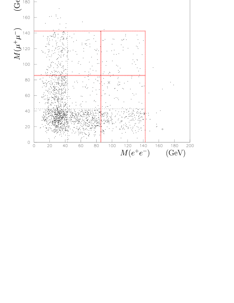
Figure 4: $M(e^{+}e^{-})$ vs. $\!M(\mu^{+}\mu^{-})$ Dalitz-like plot for MSSM Point $A$ assuming an integrated luminosity of $30\,\hbox{fb}^{-1}$. Signal events from gluino/squark production are denoted by dots, SM background events by crosses and events from other SUSY processes by open circles. Shaded bands (dashed lines) indicate kinematical endpoints expected from two-body decays (three-body decays) based on ISASUSY.

The shaded bands and dashed lines included in the plot show the expected locations of hard edges based on the –ino and slepton mass spectrum obtained from ISASUSY for Point $A$. The ${\sim}40$-$45\,\hbox{GeV}$ hard edge corresponds to the $42.8\,\hbox{GeV}$ $\widetilde{\chi}_{2}^{0}$-$\widetilde{\chi}_{1}^{0}$ mass difference. Here $\widetilde{\chi}_{2}^{0}$ is decaying through an off-shell $Z^{0}$ or slepton, with $BR(\widetilde{\chi}_{2}^{0}\rightarrow\widetilde{\chi}_{1}^{0}\ell^{+}\ell^{-})=0.245$ (very unlike the leptonic BR for the $Z^{0}$) indicating that the off-shell sleptons are playing large rôles. The other –inos decay mainly through on-mass-shell sleptons. The outer edge at ${\sim}140\,\hbox{GeV}$ agrees with the endpoint for the two-body decay chain $\widetilde{\chi}_{4}^{0}\to\tilde{\ell}\ell\to\widetilde{\chi}_{1}^{0}+\ell^{+}\ell^{-}$ (though this is the actual decay channel for this sparticle spectrum, in fact the two-body decay and three-body decay endpoints differ by less than $1\,\hbox{GeV}$ in this case). So the outer box is from $\widetilde{\chi}_{4}^{0}\widetilde{\chi}_{4}^{0}$ production and the wedge is from $\widetilde{\chi}_{2}^{0}\widetilde{\chi}_{4}^{0}$ (including an inner box from $\widetilde{\chi}_{2}^{0}\widetilde{\chi}_{2}^{0}$ production).

The population changes at ${\sim}85\,\hbox{GeV}$ inside the wedge might be interpreted as evidence for significant $\widetilde{\chi}_{2}^{0}\widetilde{\chi}_{3}^{0}$ production, or as a ‘stripe’. In fact, they are due to the latter, and are associated with the decay chain $\widetilde{\chi}_{4}^{0}\to\tilde{\ell}\ell\to\widetilde{\chi}_{2}^{0}+\ell^{+}\ell^{-}$ which happens $22.8$% of the time. The $\widetilde{\chi}_{4}^{0}$ decay chain mentioned in the last paragraph occurs $65.8$% of the time, and the remaining $10.6$% of the $\widetilde{\chi}_{4}^{0}$ decays are through $\widetilde{\chi}_{1}^{\pm}$. Note that at least some a priori knowledge of the –ino mass spectrum and decay modes is required to designate this feature a stripe, showing that such Dalitz-like plots do not always uniquely identify the underlying –ino production/decay modes. Note also that the position of this feature is given by (7), with $m_{\widetilde{\chi}_{1}^{0}}$ replaced by $m_{\widetilde{\chi}_{2}^{0}}$, which in this case is quite different from $m_{\widetilde{\chi}_{4}^{0}}-m_{\widetilde{\chi}_{2}^{0}}\doteq 100.2\,\hbox{GeV}$. Thus care must be taken before assuming that features in invariant mass plots correspond to –ino mass differences.

The designations in the last two paragraphs agree well with the percentages given in Table 3, including the ‘stripe’ assignment above as well as the absence of a $\widetilde{\chi}_{3}^{0}$-associated box or wedges in Figure 4. The events lying outside the outer box in the Dalitz-like plot are due at least in part to production modes including charginos. This was confirmed in the HERWIG simulation by checking the identities of the parent particles of the leptons in these outlying events. In addition, a sampling of such events were also found to have leptons from top-quark decays or lost leptons (i.e., they were 5 lepton events with one of the leptons being too soft to pass the minimum $E_{T}$ cut or too close to the beam axis).

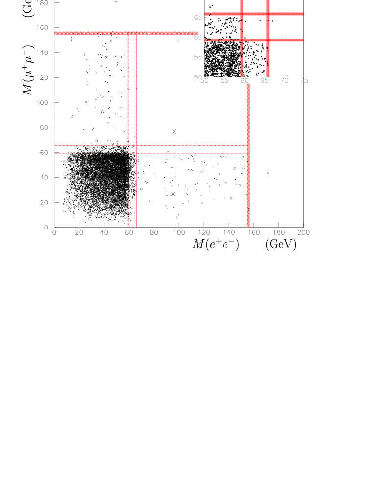
Figure 5: $M(e^{+}e^{-})$ vs. $\!M(\mu^{+}\mu^{-})$ Dalitz-like plot for MSSM Point $B$ assuming an integrated luminosity of $30\,\hbox{fb}^{-1}$. Signal events from gluino/squark production are denoted by dots, SM background events by crosses and events from other SUSY processes by open circles. Shaded bands indicate kinematical endpoints expected based on ISASUSY. The insert in the upper right corner zooms in on a critical region, and the assumed integrated luminosity is raised to $60\,\hbox{fb}^{-1}$.

Figure 5 for Point $B$ displays a somewhat sparsely-populated wedge envelope matching pattern $B$ in the right-side square of Figure 2. The interior edges for the wedge are at ${\sim}60$-$65\,\hbox{GeV}$, and event points taper off around $140$-$180\,\hbox{GeV}$. Inside this wedge is a much more densely-populated box with edges at roughly $60\,\hbox{GeV}$. A second very short-legged wedge structure is also indicated, with edges at $60\,\hbox{GeV}$ and $65\,\hbox{GeV}$. More events from a longer run time would help to clarify the structure in the crucial ($M(e^{+}e^{-}),M(\mu^{+}\mu^{-}))=$ ($60$-$65\,\hbox{GeV},60$-$65\,\hbox{GeV}$) region of the Dalitz-like plot (see insert in Figure 5). The plot bespeaks of dominant $\widetilde{\chi}_{i}^{0}\widetilde{\chi}_{i}^{0}$ production with weaker contributions from $\widetilde{\chi}_{i}^{0}\widetilde{\chi}_{j}^{0}$ and $\widetilde{\chi}_{i}^{0}\widetilde{\chi}_{k}^{0}$ ($i<j<k$) (the latter yielding the outer wedge envelope and the former the short-legged wedge). Note in the MSSM framework $i$, $j$ and $k$ must be $2$, $3$ and $4$. The short, stubby wedge tells us that two of the heavier –inos, presumably $\widetilde{\chi}_{2}^{0}$ and $\widetilde{\chi}_{3}^{0}$, are quite close in mass. This is in very good agreement with the predictions from Table 3: a densely-populated $\widetilde{\chi}_{2}^{0}\widetilde{\chi}_{2}^{0}$ box and a short, stubby $\widetilde{\chi}_{2}^{0}\widetilde{\chi}_{3}^{0}$ wedge (the $\widetilde{\chi}_{3}^{0}\widetilde{\chi}_{3}^{0}$ box is too sparsely populated to be recognised — again the ($M(e^{+}e^{-}),M(\mu^{+}\mu^{-}))=$ ($60$-$65\,\hbox{GeV},60$-$65\,\hbox{GeV}$) region of the Dalitz-like plot is seen to be crucial, with more statistics desirable to clarify the situation. Also, for this point in MSSM parameter space, $m_{\widetilde{\chi}_{3}^{0}}$ is in fact rather close to $m_{\widetilde{\chi}_{2}^{0}}$.

Shaded bands in the plot again show the expected locations of hard edges based on the –ino and slepton mass spectrum obtained from ISASUSY. Though the $62.4\,\hbox{GeV}$ $\widetilde{\chi}_{2}^{0}$-$\widetilde{\chi}_{1}^{0}$ mass difference from ISASUSY roughly fits the position of the box edges, ISASUSY also reveals that the $\widetilde{\chi}_{2}^{0}$ decays nearly always through an on-shell slepton, BR$(\widetilde{\chi}_{2}^{0}\to\tilde{\ell}\ell\to\widetilde{\chi}_{1}^{0}+\ell^{+}\ell^{-})=0.999$, with the lighter (predominantly right) and heavier (predominantly left) slepton mass eigenstates contributing about equally. Significantly, the spoiler decay modes to sneutrinos only have a suprisingly low BR of only ${\sim}10^{-3}$. Applying (7) using only the physical selectron masses (to match the HERWIG inputs) from Table 1 predicts edges at $58.5\,\hbox{GeV}$ and $59.0\,\hbox{GeV}$, confirming that the inner box is from $\widetilde{\chi}_{2}^{0}\widetilde{\chi}_{2}^{0}$ production. Again, $\widetilde{\chi}_{3}^{0}$ almost always decays via on-shell sleptons to $\widetilde{\chi}_{1}^{0}$, but now $71.6$% of the decays are into sneutrino spoiler modes yielding no charged leptons. Application of (7) now predicts endpoints at $64.8\,\hbox{GeV}$ and $65.5\,\hbox{GeV}$, about $6\,\hbox{GeV}$ less than $m_{\widetilde{\chi}_{3}^{0}}-m_{\widetilde{\chi}_{1}^{0}}$.

Note that gluino decays to $\widetilde{\chi}_{4}^{0}$ or $\widetilde{\chi}_{2}^{\pm}$ are kinematically impossible and events including a gluino decay to $\widetilde{\chi}_{1}^{\pm}$ cannot generate $4\ell$ events. Yet Table 3 says that $3.0$% of the $4\ell$ events are from $\widetilde{\chi}_{2}^{0}\widetilde{\chi}_{4}^{0}$ production and an outer $\widetilde{\chi}_{2}^{0}\widetilde{\chi}_{4}^{0}$ wedge is clearly visible in the Dalitz-like plot. This outer wedge must be due solely to production of the heavier squarks which are heavy enough to allow decays to $\widetilde{\chi}_{4}^{0}$ (the very small contribution from $\widetilde{\chi}_{4}^{0}\widetilde{\chi}_{4}^{0}$ is insufficient to generate the apparently-missing outer box). The more massive $\widetilde{\chi}_{4}^{0}$ decays $59.4$% of the time into sleptons ($26.6$% of the time into charged sleptons and $32.8$% of the time into sneutrinos). The predicted endpoints for the charged slepton decays from (7) are $153.0\,\hbox{GeV}$ and $155.4\,\hbox{GeV}$, basically giving the outer ends of the wedge envelope over $80\,\hbox{GeV}$ below the $\widetilde{\chi}_{4}^{0}$-$\widetilde{\chi}_{1}^{0}$ mass difference. Again, some if not all of the events lying outside these bounds come from processes involving charginos.

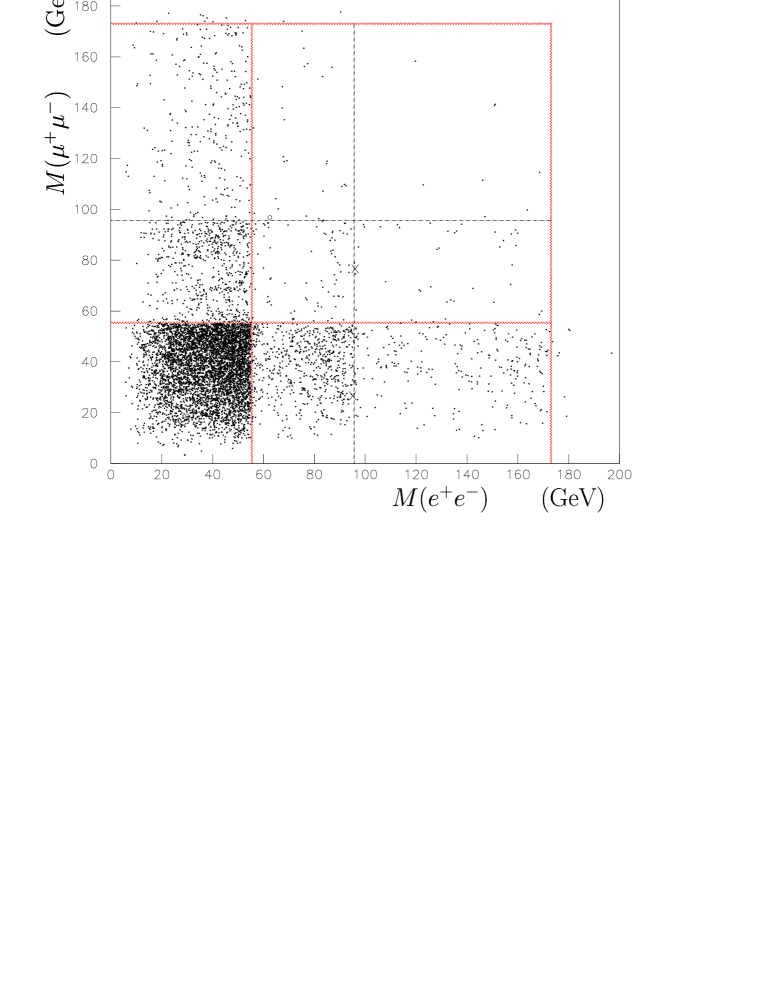
Figure 6: $M(e^{+}e^{-})$ vs. $\!M(\mu^{+}\mu^{-})$ Dalitz-like plot for MSSM Point $C$ assuming an integrated luminosity of $30\,\hbox{fb}^{-1}$. Signal events from gluino/squark production are denoted by dots, SM background events by crosses and events from other SUSY processes by open circles. Shaded bands indicate kinematical endpoints expected based on ISASUSY. The band marking the endpoint for $\widetilde{\chi}^{0}_{3}\rightarrow\tilde{\ell}^{\pm}\ell^{\mp}\rightarrow\ell^{+}\ell^{-}$ decays is quite narrow, and is drawn as a dashed line in this plot.

Lastly, Figure 6 shows the Dalitz-like plot obtained for MSSM parameter point $C$. A wedge extending out to ${\sim}175$-$180\,\hbox{GeV}$ is readily seen. The inner edges of this wedge are at ${\sim}55\,\hbox{GeV}$. Inside of this wedge is a shorter wedge with the same inner edges terminating at ${\sim}95\,\hbox{GeV}$, and in the corner a densely-populated box. Structures outside this wedge are more difficult to discern with this number of events: a box with edges at $95\,\hbox{GeV}$ is somewhat clear while a wedge with inner edges at ${\sim}95\,\hbox{GeV}$ extending out to ends at ${\sim}175$-$180\,\hbox{GeV}$ may be barely discernible. Thus this plot could be classified as either pattern $B$ or pattern $C$ according to the nomenclature introduced in the right-side square of Figure 2. The features exhibited suggest fairly dominant $\widetilde{\chi}_{i}^{0}\widetilde{\chi}_{i}^{0}$ production, but with significant contributions from $\widetilde{\chi}_{i}^{0}\widetilde{\chi}_{j}^{0}$ and $\widetilde{\chi}_{i}^{0}\widetilde{\chi}_{k}^{0}$ ($i<j<k$), and with lesser but still detectable contributions from $\widetilde{\chi}_{j}^{0}\widetilde{\chi}_{j}^{0}$ and $\widetilde{\chi}_{j}^{0}\widetilde{\chi}_{k}^{0}$. (Again, in the MSSM, $i$, $j$ and $k$ must be $2$, $3$ and $4$.)

ISASUSY numbers for the –ino and slepton mass spectrum again yield the shaded bands and dashed lines showing the expected locations of hard edges. $\widetilde{\chi}_{2}^{0}$ virtually always decays via on-shell sleptons to $\widetilde{\chi}_{1}^{0}$, $69.5$% of the time through charged sleptons and $30.5$% of the time through sneutrinos (contrast this with $\widetilde{\chi}_{2}^{0}$ decays at MSSM parameter point $B$). Again applying (7) using only the physical selectron masses (to match the HERWIG inputs) from Table 1 leads to predicted edges at $54.4\,\hbox{GeV}$ and $55.3\,\hbox{GeV}$, corroborating that the inner box is from $\widetilde{\chi}_{2}^{0}\widetilde{\chi}_{2}^{0}$ production. Note that use of more correct physical smuon masses incorporating left-right sfermion mixing would significantly widen the horizontal shaded bands in Figure 6.

Comparing the wedges in Figure 6 with the one in Figure 5, we conclude that in this case the –ino masses are not so close together. $\widetilde{\chi}_{3}^{0}$ decays via on-shell sleptons $77.6$% of the time ($17.7$% via charged sleptons and $59.9$% via sneutrinos), the rest of the time decaying via an on-shell $Z^{0}$ ($21.6$%) or a $\widetilde{\chi}_{1}^{\pm}$ ($0.7$%) or a $\widetilde{\chi}_{2}^{0}$ ($<0.1$%). The charged-slepton-mediated $\widetilde{\chi}_{3}^{0}$ decays should have endpoints at $95.8\,\hbox{GeV}$ and $95.9\,\hbox{GeV}$ (in this case the two-body endpoint is nearly equal to the $\widetilde{\chi}_{3}^{0}$-$\widetilde{\chi}_{1}^{0}$ mass difference). The $\widetilde{\chi}_{3}^{0}$ decays via $Z^{0}$ lead to a band at $91.2\,\hbox{GeV}$ also faintly visible in Figure 6. As with MSSM parameter point $B$, the sneutrino spoiler modes are much stronger (considerably stronger) in $\widetilde{\chi}_{3}^{0}$ ($\widetilde{\chi}_{4}^{0}$) decays than for $\widetilde{\chi}_{2}^{0}$ decays, suppressing contributions from the former to the Dalitz-like plot relative to the latter. Decays of $\widetilde{\chi}_{4}^{0}$ via on-shell charged sleptons (which occurs $26.9$% of the time, compared to $43.7$% of the decays being via sneutrinos) will result in edges at $172.3\,\hbox{GeV}$ and $173.0\,\hbox{GeV}$ ($10\,\hbox{GeV}$ or so below $m_{\widetilde{\chi}_{4}^{0}}-m_{\widetilde{\chi}_{1}^{0}}$). $\widetilde{\chi}_{4}^{0}$ also decays $22.3$% of the time into $\widetilde{\chi}_{1}^{\pm}W^{\mp}$ which can yield aberrant events not anticipated in the neutralinos-only framework followed here. The variation in the widths of the shaded bands due to decays occurring through the two different same-flavour sleptons, which are $4.06$, $0.44$, and $3.24\,\hbox{GeV}$, can readily be understood from the variation of (7):

$$\frac{\partial M(\ell^{+}\ell^{-})}{\partial{m_{\tilde{\ell}}}^{2}}=\frac{\Delta{m_{\tilde{\ell}}}^{2}}{2M(\ell^{+}\ell^{-})}\left(\frac{{m_{\widetilde{\chi}_{1}^{0}}}^{2}{m_{\widetilde{\chi}_{i}^{0}}}^{2}}{{m_{\tilde{\ell}}}^{4}}-1\right)\,.$$ (20)

In this case the $\widetilde{\chi}_{2}^{0}\rightarrow\widetilde{\chi}_{1}^{0}$ and $\widetilde{\chi}_{4}^{0}\rightarrow\widetilde{\chi}_{1}^{0}$ bands have similar widths, as this is inversely proportional to the endpoint yet partially compensated for by the factor in parentheses for much heavier $\widetilde{\chi}_{4}^{0}$; this factor is however very small for intermediate-mass $\widetilde{\chi}_{3}^{0}$, where ${m_{\widetilde{\chi}_{1}^{0}}}^{2}{m_{\widetilde{\chi}_{3}^{0}}}^{2}/{m_{\tilde{\ell}}}^{4}\approx 1$, hence the relatively thin $\widetilde{\chi}_{3}^{0}\rightarrow\widetilde{\chi}_{1}^{0}$ band.

Summarizing, the predicted endpoints from charged-slepton-mediated decays of $\widetilde{\chi}_{3}^{0}$ and $\widetilde{\chi}_{4}^{0}$ affirm that the shorter (longer) wedge is from $\widetilde{\chi}_{2}^{0}\widetilde{\chi}_{3}^{0}$ ($\widetilde{\chi}_{2}^{0}\widetilde{\chi}_{4}^{0}$) production. The more faintly discernible box with edges at ${\sim}95\,\hbox{GeV}$ is attributed to $\widetilde{\chi}_{3}^{0}\widetilde{\chi}_{3}^{0}$ production, the even more faint wedge of which this box is the corner is from $\widetilde{\chi}_{3}^{0}\widetilde{\chi}_{4}^{0}$ production, and the few events in the upper-left corner of the plot are presumably from $\widetilde{\chi}_{4}^{0}\widetilde{\chi}_{4}^{0}$ production. The relative percentages of $4\ell$ events given in Table 3 agrees fairly well with the densities of points seen in the associated features in Figure 6.

It is interesting to see how effectively the relative –ino pair contributions can be extracted from the Dalitz-like plot. Assuming some knowledge of the dilepton invariant mass distribution, an estimate of the ratio of the different –ino pair production rates (stemming from the gluino/squark BRs to the different –inos) is obtainable from counting the total number of points in each region of the Dalitz plot and then taking the ratio. Approximating the distributions as being exactly triangular (see  [10]), and taking the endpoint locations noted in the preceding paragraphs as $55\,\hbox{GeV}$ , $96\,\hbox{GeV}$ and $173\,\hbox{GeV}$, the following rate comparison can be extracted:

$$r_{22}:r_{23}:r_{24}:r_{33}:r_{34}:r_{44}=431:118:59:15.5:9.4:1\;\;\;,$$ (21)

where $r_{ij}$ is the rate from $\widetilde{\chi}_{i}^{0}\widetilde{\chi}_{j}^{0}$ production, or, considering just the the three wedges, $r_{23}:r_{24}:r_{34}=12.3:6.3:1\,$. Compare these values to the results obtained earlier from Table 3

$$r_{22}:r_{33}:r_{44}=131.5:1.3:1\;\;\hbox{and}\;\;r_{23}:r_{24}:r_{34}=10.2:9.6:1\;\;.$$ (22)

Little more than crude agreement is discernible; bear in mind though that, as noted earlier, discrepancies may be reasonably expected in comparing all-inclusive $4\ell$ rates with $e^{+}e^{-}{\mu}^{+}{\mu}^{-}$ rates after cuts. The assumption of strictly triangular population profiles is also certainly somewhat inaccurate. And, at least with modest statistics (i.e., with only results from the first year or two of running for the LHC), there will be significant imprecision in pinpointing the locations of the endpoints (the main source of uncertainty in the calculation if the triangular distribution assumption is viable). One factor that is not an important concern at this MSSM parameter point is contamination from chargino-related events; but, said contamination could skew such a calculation at other MSSM points (as, for instance, Point $A$).

If $r_{ij}=2r_{i}r_{j}$ is now assumed to be valid (note though the afore-mentioned serious caveats to this assumption), the relative individual production times leptonic BRs are obtainable: $r_{2}:r_{3}:r_{4}=12.3:1.6:1\;$ (using $r_{23}$, $r_{34}$ and $r_{22}$ or $r_{24}$ as inputs) or $r_{2}:r_{3}:r_{4}=12.6:4.7:1\;$ (using $r_{23}$, $r_{34}$ and $r_{44}$ as inputs). The extent to which these two results disagree could (as before for the inclusive $4\ell$ results) be interpreted as implying significant contributions from squark-production (though the inaccuracy of the triangular distribution assumption may also be a factor). Recall inclusive $4\ell$ results were $r_{2}:r_{3}:r_{4}=19.00:1.04:1$ (using $r_{23}$, $r_{34}$ and $r_{24}$ as inputs) and $r_{2}:r_{3}:r_{4}=11.47:1.16:1$ (using $r_{22}$, $r_{33}$ and $r_{44}$ as inputs). Apparently, dynamical information from the densities of events in the Dalitz-like plot’s various geometrical components may be more difficult to extract than the kinematical information contained in the location of the hard edges. However, more sophisticated statistical analyses may be expected to yield better results.

Next contrast the information apparent in the Dalitz-like plots with that readily obtainable from the more traditional one-dimensional projections shown in Figure 7. Notice how similar the results for Points $B$ and $C$ appear in Figure 7, while Figure 5 and Figure 6 are quite different. Note also in this case the sharp drops observed would only be sufficient to identify which –inos are being produced, not which –ino pairs are being produced.

Figure 7: One-dimensional projection of Figures 4-6 for MSSM Points $A$, $B$ and $C$ assuming an integrated luminosity of $30\,\hbox{fb}^{-1}$. Information about the decay topology is lost in such projections.

Concluding Remarks

Production of pairs of new heavy particle states $X_{i}X_{j}$ at hadron colliders has been studied emphasising the simple topological forms expected in certain two-dimensional Dalitz-like plots. It is assumed the heavy particles decay into pairs of SM particles (with the possible addition of substantial amounts of missing energy), yielding final states of the form $x\bar{x}\,+\,y\bar{y}\,\,(+\,\hbox to0.0pt{\hbox to7.95831pt{\hfil/\hfil}\hss}E$), where in this work $x$ and $y$ are taken to be distinct SM fermions. Given a sufficient number of events, the observed topology (a ‘box’ or a ‘wedge’) clearly indicates whether or not $X_{i}$ and $X_{j}$ are identical particles. When simultaneous production of more than one pair of new particles is possible within a model, a more extensive set of topologies constructed from boxes and wedges (possibly with overlayed ‘stripes’) is obtained. A likelihood function indicating how well the a set of data points fits each possibility can be readily constructed if visual inspection does not suffice. The particular set of shapes the data sample should be thus compared to is of course model dependent.

Though we wish to stress the general applicability of this technique to a fairly wide range of beyond-the-SM scenarios, application to $R$-parity conserving SUSY models readily springs to mind. Thus the pair production of heavy MSSM neutralinos (excluding the lightest one, the LSP), with the subsequent decay of each –ino into a pair of leptons to aid identification, has been examined in detail. Here a fairly sizable number of distinct topological shapes is obtainable. This work then further specialises to –ino pairs produced in gluino/squark decays, most likely to be the dominant mode of –ino production at the LHC — if gluinos and/or squarks are relatively light. The number of possible topologies may be substantially reduced when this is the production mechanism compared to the EW production mechanisms which contain an –ino–ino-$S$ vertex if squark production does not re-introduce complexity. This was examined in some detail including possible tests of simulation results that may indicate the significance of squark production (and distinguish it from gluino pair production). Neutralino results thus obtained might be compared to those from charge asymmetries possible in samples of like-sign dilepton events from chargino pair production  [13].

The ‘hard edges’ seen in a Dalitz-like plot yield information on the –ino mass differences as well as the identities of –inos participating in the decays (though it should be emphasised that the endpoints certainly need not equal the mass difference of two –inos if on-mass-shell sleptons are involved in the decay chains), while comparing the relative densities of regions populated by different $X_{i}X_{j}$ production channels or combinations of channels has the potential to provide information on the relative production cross sections times leptonic BRs of these channels. We found simulation results from HERWIG for three distinctive points in MSSM parameter space (including cuts that nearly eliminate the backgrounds and a realistic detector simulation) clearly closely tract the partial results we obtained at these points by ‘hand’-calculations based on the ISASUSY inputs. It is apparent from the Dalitz-like plots shown that this includes a substantial amount of information not available from a one-dimensional plot that just lumps together $e^{+}e^{-}$ and ${\mu}^{+}{\mu}^{-}$ invariant masses. Upcoming consideration of –ino pair production via heavy MSSM Higgs bosons  [7], which also can have quite substantial rates in favourable regions of MSSM parameter space, will further expand the extra information obtainable from the two-dimensional Dalitz-like plot and thus should prove very exciting. Of course such analyses only incorporate mixed leptonic decays — ($e^{+}e^{-}{\mu}^{+}{\mu}^{-}$ events, but not $e^{+}e^{-}e^{+}e^{-}$ or ${\mu}^{+}{\mu}^{-}{\mu}^{+}{\mu}^{-}$ events).

We also note that it is possible to make lego-style 3-dimensional plots with $M(x\bar{x})$ and $M(y\bar{y})$ along two axes and the binned number of events along a third axis. Figures obtained in this way were not found particularly illuminating for the specific processes and MSSM parameter points studied here (and with the modest amount of integrated luminosity assumed), but may be more useful in other studies.

How far this method can go toward aiding reconstruction of the –ino mass spectrum will depend on particulars of the point in the MSSM parameter space nature chooses, but clearly very significant information may be extracted. Given that an $e^{+}e^{-}$ linear collider with a centre-of-mass energy beyond that of LEP 2 is not expected for some time, it is crucial to seek the optimal methods for disentangling the –inos produced at the LHC. Further, information on the heavier –ino states may prove crucial in deciding the reach of a future linear collider to perform the more precise measurements surely required.

Appendix

The schematic Dalitz-like plot shown in the right square of Figure 2 is a collection of 6 observables (there labeled as regions $\alpha,\beta,...\kappa$) from which the production times leptonic BR values for the various –ino pairs, $r_{ij}$ ($i,j=2,3,4$) may be extracted. First, a triangular distribution of events is assumed for each –ino –ino mode:

$$r_{ij}={\cal K}\int dx\int dy\;x\,y$$ (23)

where ${\cal K}$ is a normalization constant that will drop out of the calculation. Now each region of the Dalitz plot contains events attributable to one or more of the modes $r_{ij}$. The six different regions therefore correspond to different combinations of the $r_{ij}$; which may be written as

$$v_{1}={\cal M}v_{2}\;,$$ (24)

with vectors $v_{1}=\left(\alpha,2\beta,2\gamma,\delta,2\eta,\kappa\right)$ and $v_{2}=\left(r_{22},r_{23},r_{24},r_{33},r_{34},r_{44}\right)$, and the matrix

$${\cal M}=\left(\begin{array}[]{c c c c c c}1&a&b&c&d&e\\ 0&f&g&h&i&j\\ 0&0&k&0&l&m\\ 0&0&0&n&o&p\\ 0&0&0&0&q&r\\ 0&0&0&0&0&s\\ \end{array}\right)$$ (25)

where $a,b,c,...s$ are numbers between 0 and 1 which represent the fraction of events from $r_{ij}$ in a particular region; for example, $s=\frac{\int^{E_{2}}_{E_{1}}dx\int^{E_{2}}_{E_{1}}dy\;x\,y}{\int^{E_{2}}_{0}dx\int^{E_{2}}_{0}dy\;x\,y}=\left[1-\left(\frac{E_{1}}{E_{2}}\right)^{2}\right]^{2}$ with $E_{0,1,2}$ being the three kinematical endpoints in the figure. Elements in each column of the matrix ${\cal M}$ must sum to unity. Now defining $x=\left(\frac{E_{0}}{E_{1}}\right)^{2}$, $y=\left(\frac{E_{0}}{E_{2}}\right)^{2}$ and $z=\left(\frac{E_{1}}{E_{2}}\right)^{2}$ yields
$a=x$ $b=y$ $c=x^{2}$ $d=xy$ $e=y^{2}$ $f=1-x$ $g=z-y$ $h=2x(1-x)$ $i=2y(1-x)$ $j=2y(z-y)$ $k=1-z$ $l=x(1-z)$ $m=2y(1-z)$ $n=(1-x)^{2}$ $o=(1-x)(z-y)$ $p=(z-y)^{2}$ $q=(1-x)(1-z)$ $r=2(1-z)(z-y)$ $s=(1-z)^{2}$ The linear system of equations is now easily solved for the individual rates $r_{ij}$.

References

- [1]
- [2] For reviews of the MSSM and SUSY, see: G. Kane, ed., Perspectives on Supersymmetry (World Scientific, Singapore, 1998); M. Drees and S.P. Martin, in Electroweak Symmetry Breaking and New Physics at the TeV Scale (World Scientific, Singapore, 1996), T.L. Barklow, S. Dawson, H.E. Haber, and J.L. Siegrist (eds.), pages 146–215 (hep-ph/9504324); H. Baer et al., ibid., pages 216–286 (hep-ph/9503479); H.E. Haber, Nucl. Phys. Proc. Suppl. 62 (1998) 469 (hep-ph/9709450).
- [3] N. Arkani-Hamed, A. G. Cohen, T. Gregoire and J. G. Wacker, JHEP 08 (2002) 020.
- [4] The original Dalitz plot papers are: R.H. Dalitz, Phil. Mag. 44 (1953) 1068; E. Fabri, Nuovo Cimento 1 (1954) 479. For examples of resonance-hunting using Dalitz plots see, for example, J. Shafer, J. Murray and D. Huwe, Phys. Rev. Lett. 10 (1963) 176; M. Ferro Luzzi et al., Nuovo Cimento 36 (1965) 1101.
- [5] K.A. Assamagan et al., hep-ph/0406152.
- [6] W. Beenakker, R. Hopker, M. Spira and P.M. Zerwas, Nucl. Phys. B 492 (1997) 51.
- [7] M. Bisset, N. Kersting, J. Li, F. Moortgat and S. Moretti, in preparation.
- [8] H. Baer, C-H. Chen, F. Paige and X. Tata, Phys. Rev. D 53 (1996) 6241.
- [9] F. E. Paige, hep-ph/9609373; I. Hinchliffe, F.E. Paige, M.D. Shapiro, J. Söderqvist and W. Yao, Phys. Rev. D 55 (1997) 5520.
- [10] H. Bachacou, I. Hinchliffe and F.E. Paige, Phys. Rev. D 62 (2000) 015009.
- [11] J.G. Branson, D. Denegri, I. Hinchliffe, F. Gianotti, F.E. Paige and P. Sphicas, hep-ph/9609373.
- [12] D. Denegri, W. Majerotto and L. Rurua, Phys. Rev. D 58 (1998) 095010, ibid., 60 (1999) 035008.
- [13] H. Baer, C-H. Chen, M. Drees, F. Paige and X. Tata, Phys. Rev. D 59 (1999) 055014.
- [14] H. Baer, M. Bisset, D. Dicus, C. Kao and X. Tata, Phys. Rev. D 47 (1993) 1062; H. Baer, M. Bisset, C. Kao and X. Tata, Phys. Rev. D 50 (1994) 316.
- [15] F. Moortgat, S. Abdullin and D. Denegri, hep-ph/0112046.
- [16] H. Baer and X. Tata, Phys. Rev. D 47 (1993) 2739.
- [17] See: LEP SUSY Working Group web page, http://www.cern.ch/LEPSUSY/.
- [18] G. Corcella et al., JHEP 0101 (2001) 010, hep-ph/0210213; S. Moretti, K. Odagiri, P. Richardson, M.H. Seymour and B.R. Webber, JHEP 0204 (2002) 028.
- [19] J. Pumplin et al. (CTEQ Collaboration) (CTEQ6), JHEP 0207 (2002) 012, ibid, 0310 (2003) 046; H.L. Lai et al. (CTEQ Collaboration) (CTEQ5), Eur. Phys. J. C 12 (2000) 375.
- [20] H. Baer, F.E. Paige, S.D. Protopopescu and X. Tata, hep-ph/0001086, hep-ph/0312045.