Branching ratio and CP violation of $B_{s}\to\pi K$ decays
in the perturbative QCD approach

Abstract

In the framework of perturbative QCD approach, we calculate the branching ratio and CP asymmetry for $B_{s}^{0}(\bar{B}_{s})\to\pi^{\pm}K^{\mp}$ and $B_{s}(\bar{B}_{s})\rightarrow\pi^{0}\bar{K}^{0}(K^{0})$ decays. Besides the usual factorizable diagrams, both non-factorizable and annihilation type contributions are taken into account. We find that (a) the branching ratio of $B_{s}^{0}(\bar{B}_{s})\to\pi^{\pm}K^{\mp}$ is about $(6-10)\times 10^{-6}$; $Br(B_{s}(\bar{B}_{s})\rightarrow\pi^{0}\bar{K}^{0}(K^{0}))$ about $(1-3)\times 10^{-7}$; and (b) there are large CP asymmetries in the two processes, which can be tested in the near future LHC-b experiments at CERN and BTeV experiments at Fermilab.

I Introduction

The rare charmless B meson decays arouse more and more interest, since it is a good place for testing the Standard Model (SM), studying CP violation and looking for possible new physics beyond the SM. Since 1999, the B factories in KEK and SLAC collect more and more data sample of rare B decays. In the future CERN Large Hadron Collider beauty experiments (LHC-b), the heavier $B_{s}$ and $B_{c}$ mesons can also be produced. With the bright hope in LHC-b experiments and BTeV experiments at Fermilab, following a previous study of $B_{s}\rightarrow\pi^{+}\pi^{-}$ decay 1 , we continue to investigate other $B_{s}$ rare decays.

The most difficult problem in theoretical calculation of non-leptonic $B$ decays is the calculation of hadronic matrix element. The widely used method is the factorization approach (FA) 2 . It is a great success in explaining the branching ratio of many decays 3 ; 5 , although it is a very simple method. In order to improve the theoretical precision, QCD factorization 6 and perturbative QCD approach (PQCD) 7 are developed. Perturbative QCD factorization theorem for exclusive heavy-meson decays has been proved some time ago, and applied to semi-leptonic $B\to D(\pi)l\nu$ decays 7 , the non-leptonic $B\to K\pi$ 15 , $\pi\pi$ 8 decays. PQCD is a method to factorize hard components from a QCD process, which can be treated by perturbation theory. Non-perturbative parts are organized in the form of universal hadron light cone wave functions, which can be extracted from experiments or constrained by lattice calculations and QCD sum rules. More information about PQCD approach can be found in 7 ; pqcd .

In this paper, we would like to study the $B_{s}^{0}(\bar{B}_{s})\to\pi^{\pm}K^{\mp}$ and $B_{s}(\bar{B}_{s})\rightarrow\pi^{0}\bar{K}^{0}(K^{0})$ decays in the perturbative QCD approach. In our calculation, we ignore the soft final state interaction because there are not many resonances near the energy region of $B_{s}$ mass. Our theoretical formulas for the decay $B_{s}\to\pi K$ in PQCD framework are given in the next section. In section III, we give the numerical results of the branching ratio of $B_{s}\to\pi K$ and discussions for CP asymmetries and the form factor of $B_{s}\to K$ etc. At last, we give a short summary in section IV.

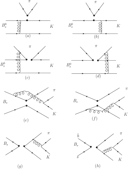
Figure 1: The lowest order diagrams for $B_{s}^{0}\to\pi K$ decay.

II Perturbative calculations

For decay $B_{s}\to\pi K$, the related effective Hamiltonian is given by 9

$$H_{\mathrm{eff}}=\frac{G_{F}}{\sqrt{2}}\left\{V_{ud}V_{ub}^{*}\left[C_{1}(\mu)O_{1}(\mu)+C_{2}(\mu)O_{2}(\mu)\right]-V_{tb}^{*}V_{td}\sum_{i=3}^{10}C_{i}(\mu)O_{i}(\mu)\right\},$$ (1)

where $C_{i}(\mu)(i=1,\cdots,10)$ are Wilson coefficients at the renormalization scale $\mu$ and $O_{i}(i=1,\cdots,10)$ are the four quark operators

$$\begin{array}[]{ll}O_{1}=(\bar{b}_{i}u_{j})_{V-A}(\bar{u}_{j}d_{i})_{V-A},&O_{2}=(\bar{b}_{i}u_{i})_{V-A}(\bar{u}_{j}d_{j})_{V-A},\\ O_{3}=(\bar{b}_{i}d_{i})_{V-A}\sum_{q}(\bar{q}_{j}q_{j})_{V-A},&O_{4}=(\bar{b}_{i}d_{j})_{V-A}\sum_{q}(\bar{q}_{j}q_{i})_{V-A},\\ O_{5}=(\bar{b}_{i}d_{i})_{V-A}\sum_{q}(\bar{q}_{j}q_{j})_{V+A},&O_{6}=(\bar{b}_{i}d_{j})_{V-A}\sum_{q}(\bar{q}_{j}q_{i})_{V+A},\\ O_{7}=\frac{3}{2}(\bar{b}_{i}d_{i})_{V-A}\sum_{q}e_{q}(\bar{q}_{j}q_{j})_{V+A},&O_{8}=\frac{3}{2}(\bar{b}_{i}d_{j})_{V-A}\sum_{q}e_{q}(\bar{q}_{j}q_{i})_{V+A},\\ O_{9}=\frac{3}{2}(\bar{b}_{i}d_{i})_{V-A}\sum_{q}e_{q}(\bar{q}_{j}q_{j})_{V-A},&O_{10}=\frac{3}{2}(\bar{b}_{i}d_{j})_{V-A}\sum_{q}e_{q}(\bar{q}_{j}q_{i})_{V-A}.\end{array}$$ (2)

Here $i$ and $j$ are $SU(3)$ color indices; the sum over $q$ runs over the quark fields that are active at the scale $\mu=O(m_{b})$, i.e., $q\in\{u,d,s,c,b\}$. Operators $O_{1},O_{2}$ come from tree level interaction, while $O_{3},O_{4},O_{5},O_{6}$ are QCD-Penguins operators and $O_{7},O_{8},O_{9},O_{10}$ come from electroweak-penguins.

Working at the rest frame of $B_{s}$ meson, we take kaon and pion masses $M_{K}\sim M_{\pi}\sim 0$, which are much smaller than $M_{B_{s}}$. In the light-cone coordinates, the momenta of the $B_{s}$, $K$ and $\pi$ can be written as :

$$P_{1}=\frac{M_{B}}{\sqrt{2}}(1,1,{\bf 0}_{T}),\ \ \ P_{2}=\frac{M_{B}}{\sqrt{2}}(0,1,{\bf 0}_{T}),\ \ \ P_{3}=\frac{M_{B}}{\sqrt{2}}(1,0,{\bf 0}_{T}).$$ (3)

Denoting the light (anti-)quark momenta in $B$, $K$ and $\pi$ as $k_{1}$, $k_{2}$ and $k_{3}$, respectively, we can choose:

$$k_{1}=(x_{1}p_{1}^{+},0,{\bf k}_{1T}),~{}~{}~{}k_{2}=(0,x_{2}p_{2}^{-},{\bf k}_{2T}),~{}~{}~{}k_{3}=(x_{3}p_{3}^{+},0,{\bf k}_{3T}).$$ (4)

In the following, we start to compute the decay amplitudes of $B_{s}\rightarrow\pi K$.

According to effective Hamiltonian (1), we draw the lowest order diagrams of $B_{s}\rightarrow\pi K$ in Fig. 1. Let us first look at the usual factorizable diagrams (a) and (b). they can give the $B_{s}\to K$ form factor if take away the Wilson coefficients. The operators $O_{1},O_{2},O_{3},O_{4},O_{9}$ and $O_{10}$ are $(V-A)(V-A)$ currents, and the sum of their contributions is given by

$$F_{e}[C]=16\pi C_{F}M_{B}^{2}\int_{0}^{1}\!\!\!dx_{1}dx_{2}\int_{0}^{\infty}\!\!\!\!\!b_{1}db_{1}\,b_{2}db_{2}\ \phi_{B}(x_{1},b_{1})\\ \times\bigl{\{}[(2-x_{2})\phi_{K}^{A}(x_{2})-r_{K}(1-2x_{2})\phi_{K}^{P}(x_{2})\\ +r_{K}(1-2x_{2})\phi_{K}^{T}(x_{2})]\alpha_{s}(t_{a}^{1})h_{a}(x_{1},1-x_{2},b_{1},b_{2})\exp[-S_{B}(t_{a}^{1})-S_{K}(t_{a}^{1})]C(t_{a}^{1})\\ +2r_{K}\phi_{K}^{P}(x_{2})\alpha_{s}(t_{a}^{2})h_{a}(1-x_{2},x_{1},b_{2},b_{1})\exp[-S_{B}(t_{a}^{2})-S_{K}(t_{a}^{2})]C(t_{a}^{2})\bigr{\}},$$ (5)

where $r_{\pi}=m_{0\pi}/m_{B}=m_{\pi}^{2}/[m_{B}(m_{u}+m_{d})]$, $r_{K}=m_{0K}/m_{B}=m_{K}^{2}/[m_{B}(m_{s}+m_{u})]$. $C_{F}=4/3$ is the group factor of the $SU(3)_{c}$ gauge group. The expressions of the meson distribution amplitudes $\phi_{M}$, the Sudakov factor $S_{X}(t_{i})(X=B_{s},K,\pi)$, and the functions $h_{a}$ are given in the appendix. In above formula, the Wilson coefficients $C(t)$ of the corresponding operators are process dependent.

The operator $O_{5},O_{6},O_{7},O_{8}$ have the structure of $(V-A)(V+A)$, their amplitude is

$$F_{e}^{P}[C]=32\pi C_{F}M_{B}^{2}r_{\pi}\int_{0}^{1}\!\!\!dx_{1}dx_{2}\int_{0}^{\infty}\!\!\!\!\!b_{1}db_{1}\,b_{2}db_{2}\ \phi_{B}(x_{1},b_{1})\\ \times\bigl{\{}[\phi_{K}^{A}(x_{2})-r_{K}(x_{2}-3)\phi_{K}^{P}(x_{2})\\ +r_{K}(1-x_{2})\phi_{K}^{T}(x_{2})]\alpha_{s}(t_{a}^{1})h_{a}(x_{1},1-x_{2},b_{1},b_{2})\exp[-S_{B}(t_{a}^{1})-S_{K}(t_{a}^{1})]C(t_{a}^{1})\\ +2r_{K}\phi_{K}^{P}(x_{2})\alpha_{s}(t_{a}^{2})h_{a}(1-x_{2},x_{1},b_{2},b_{1})\exp[-S_{B}(t_{a}^{2})-S_{K}(t_{a}^{2})]C(t_{a}^{2})\bigr{\}}.$$ (6)

For the non-factorizable diagrams (c) and (d), all three meson wave functions are involved. Using $\delta$ function $\delta(b_{1}-b_{3})$, the integration of $b_{1}$ can be preformed easily. For the $(V-A)(V-A)$ operators the result is:

$$M_{e}[C]=-\frac{32}{3}\pi C_{F}\sqrt{2N_{c}}M_{B}^{2}\int_{0}^{1}\!\!\!dx_{1}dx_{2}dx_{3}\int_{0}^{\infty}\!\!\!\!\!b_{2}db_{2}\ b_{3}db_{3}\ \phi_{B}(x_{1},b_{3})\\ \times\bigl{\{}[(x_{3}-1)\phi_{\pi}^{A}(x_{3})\phi_{K}^{A}(x_{2})+r_{K}(1-x_{2})\phi_{\pi}^{A}(x_{3})\phi_{K}^{P}(x_{2})+r_{K}(1-x_{2})\phi_{\pi}^{A}(x_{3})\phi_{K}^{T}(x_{2})]C(t_{c}^{1})\\ \alpha_{s}(t_{c}^{1})h_{c}^{(1)}(x_{1},x_{2},x_{3},b_{2},b_{3})\exp[-S_{B}(t_{c}^{1})-S_{\pi}(t_{c}^{1})-S_{K}(t_{c}^{1})]-[(x_{2}-x_{3}-1)\phi_{\pi}^{A}(x_{3})\phi_{K}^{A}(x_{2})\\ +r_{K}(1-x_{2})\phi_{\pi}^{A}(x_{3})\phi_{K}^{P}(x_{2})-r_{K}(1-x_{2})\phi_{\pi}^{A}(x_{3})\phi_{K}^{T}(x_{2})]C(t_{c}^{2})\\ \alpha_{s}(t_{c}^{2})h_{c}^{(2)}(x_{1},x_{2},x_{3},b_{2},b_{3})\exp[-S_{B}(t_{c}^{2})-S_{\pi}(t_{c}^{2})-S_{K}(t_{c}^{2})]\bigr{\}}.$$ (7)

For the$(V-A)(V+A)$ operators, the formula is:

$$M_{e}^{P}[C]=-\frac{32}{3}\pi C_{F}\sqrt{2N_{c}}M_{B}^{2}r_{\pi}\int_{0}^{1}\!\!\!dx_{1}dx_{2}dx_{3}\int_{0}^{\infty}\!\!\!\!\!b_{2}db_{2}\ b_{3}db_{3}\ \phi_{B}(x_{1},b_{3})\\ \times\bigl{\{}[r_{K}(x_{2}+x_{3}-2)\phi_{\pi}^{P}(x_{3})\phi_{K}^{P}(x_{2})-r_{K}(x_{2}-x_{3})\phi_{\pi}^{P}(x_{3})\phi_{K}^{T}(x_{2})-r_{K}(x_{2}-x_{3})\phi_{\pi}^{T}(x_{3})\phi_{K}^{P}(x_{2})\\ -r_{K}(2-x_{2}-x_{3})\phi_{\pi}^{T}(x_{3})\phi_{K}^{T}(x_{2})-(1-x_{3})\phi_{\pi}^{P}(x_{3})\phi_{K}^{A}(x_{2})-(1-x_{3})\phi_{\pi}^{T}(x_{3})\phi_{K}^{A}(x_{2})]C(t_{c}^{1})\\ \alpha_{s}(t_{c}^{1})h_{c}^{(1)}(x_{1},x_{2},x_{3},b_{2},b_{3})\exp[-S_{B}(t_{c}^{1})-S_{\pi}(t_{c}^{1})-S_{K}(t_{c}^{1})]+[r_{K}(1-x_{2}+x_{3})\phi_{\pi}^{P}(x_{3})\phi_{K}^{P}(x_{2})\\ +r_{K}(x_{2}+x_{3}-1)\phi_{\pi}^{P}(x_{3})\phi_{K}^{T}(x_{2})-r_{K}(x_{2}+x_{3}-1)\phi_{\pi}^{T}(x_{3})\phi_{K}^{P}(x_{2})-r_{K}(1-x_{2}+x_{3})\phi_{\pi}^{T}(x_{3})\phi_{K}^{T}(x_{2})\\ +x_{3}\phi_{\pi}^{P}(x_{3})\phi_{K}^{A}(x_{2})-x_{3}\phi_{\pi}^{T}(x_{3})\phi_{K}^{A}(x_{2})]C(t_{c}^{2})\\ \alpha_{s}(t_{c}^{2})h_{c}^{(2)}(x_{1},x_{2},x_{3},b_{2},b_{3})\exp[-S_{B}(t_{c}^{2})-S_{\pi}(t_{c}^{2})-S_{K}(t_{c}^{2})]\bigr{\}}.$$ (8)

Similar to (c),(d), the annihilation diagrams (e) and (f) also involve all three meson wave functions. Here we have two kinds of amplitudes, $M_{a}$ is the contribution containing the operator of type $(V-A)(V-A)$, and $M_{a}^{P}$ is the contribution containing the operator of type $(V-A)(V+A)$.

$$M_{a}[C]=-\frac{32}{3}\pi C_{F}\sqrt{2N_{c}}M_{B}^{2}\int_{0}^{1}\!\!\!dx_{1}dx_{2}dx_{3}\int_{0}^{\infty}\!\!\!\!\!b_{1}db_{1}\ b_{2}db_{2}\ \phi_{B}(x_{1},b_{1})\\ \times\bigl{\{}[x_{3}\phi_{\pi}^{A}(x_{3})\phi_{K}^{A}(x_{2})+r_{\pi}r_{K}(2+x_{2}+x_{3})\phi_{\pi}^{P}(x_{3})\phi_{K}^{P}(x_{2})-r_{\pi}r_{K}(x_{2}-x_{3})\phi_{\pi}^{P}(x_{3})\phi_{K}^{T}(x_{2})\\ -r_{\pi}r_{K}(x_{2}-x_{3})\phi_{\pi}^{T}(x_{3})\phi_{K}^{P}(x_{2})-r_{\pi}r_{K}(2-x_{2}-x_{3})\phi_{\pi}^{T}(x_{3})\phi_{K}^{T}(x_{2})]C(t_{e}^{1})\\ \alpha_{s}(t_{e}^{1})h_{e}^{(1)}(x_{1},x_{2},x_{3},b_{1},b_{2})\exp[-S_{B}(t_{e}^{1})-S_{\pi}(t_{e}^{1})-S_{K}(t_{e}^{1})]-[x_{2}\phi_{\pi}^{A}(x_{3})\phi_{K}^{A}(x_{2})\\ +r_{\pi}r_{K}(x_{2}+x_{3})\phi_{\pi}^{P}(x_{3})\phi_{K}^{P}(x_{2})+r_{\pi}r_{K}(x_{2}-x_{3})\phi_{\pi}^{P}(x_{3})\phi_{K}^{T}(x_{2})+r_{\pi}r_{K}(x_{2}-x_{3})\phi_{\pi}^{T}(x_{3})\phi_{K}^{P}(x_{2})\\ +r_{\pi}r_{K}(x_{2}+x_{3})\phi_{\pi}^{T}(x_{3})\phi_{K}^{T}(x_{2})]C(t_{e}^{2})\\ \alpha_{s}(t_{e}^{2})h_{e}^{(2)}(x_{1},x_{2},x_{3},b_{1},b_{2})\exp[-S_{B}(t_{e}^{2})-S_{\pi}(t_{e}^{2})-S_{K}(t_{e}^{2})]\bigr{\}},$$ (9)

$$M_{a}^{P}[C]=-\frac{32}{3}\pi C_{F}\sqrt{2N_{c}}M_{B}^{2}\int_{0}^{1}\!\!\!dx_{1}dx_{2}dx_{3}\int_{0}^{\infty}\!\!\!\!\!b_{1}db_{1}\ b_{2}db_{2}\ \phi_{B}(x_{1},b_{1})\\ \times\bigl{\{}[r_{K}(2-x_{2})\phi_{\pi}^{A}(x_{3})\phi_{K}^{P}(x_{2})+r_{K}(2-x_{2})\phi_{\pi}^{A}(x_{3})\phi_{K}^{T}(x_{2})-r_{\pi}(2-x_{3})\phi_{\pi}^{P}(x_{3})\phi_{K}^{A}(x_{2})\\ -r_{\pi}(2-x_{3})\phi_{\pi}^{T}(x_{3})\phi_{K}^{A}(x_{2})]C(t_{e}^{1})\\ \alpha_{s}(t_{e}^{1})h_{e}^{(1)}(x_{1},x_{2},x_{3},b_{1},b_{2})\exp[-S_{B}(t_{e}^{1})-S_{\pi}(t_{e}^{1})-S_{K}(t_{e}^{1})]+[r_{K}x_{2}\phi_{\pi}^{A}(x_{3})\phi_{K}^{P}(x_{2})\\ +r_{K}x_{2}\phi_{\pi}^{A}(x_{3})\phi_{K}^{T}(x_{2})-r_{\pi}x_{3}\phi_{\pi}^{P}(x_{3})\phi_{K}^{A}(x_{2})-r_{\pi}x_{3}\phi_{\pi}^{T}(x_{3})\phi_{K}^{A}(x_{2})]C(t_{e}^{2})\\ \alpha_{s}(t_{e}^{2})h_{e}^{(2)}(x_{1},x_{2},x_{3},b_{1},b_{2})\exp[-S_{B}(t_{e}^{2})-S_{\pi}(t_{e}^{2})-S_{K}(t_{e}^{2})]\bigr{\}}.$$ (10)

The factorizable annihilation diagrams (g) and (h) involve only two light mesons wave functions. $F_{a}$ is for $(V-A)(V-A)$ type operators, and $F_{a}^{P}$ is for $(V-A)(V+A)$ type operators:

$$F_{a}[C]=16\pi C_{F}M_{B}^{2}\int_{0}^{1}\!\!\!dx_{2}dx_{3}\int_{0}^{\infty}\!\!\!\!\!b_{2}db_{2}\,b_{3}db_{3}\ \\ \times\bigl{\{}[-x_{2}\phi_{\pi}^{A}(x_{3})\phi_{K}^{A}(x_{2})-2r_{\pi}r_{K}(1+x_{2})\phi_{\pi}^{P}(x_{3})\phi_{K}^{P}(x_{2})+2r_{\pi}r_{K}(1-x_{2})\phi_{\pi}^{P}(x_{3})\phi_{K}^{T}(x_{2})]\\ \alpha_{s}(t_{g}^{1})h_{g}(x_{2},x_{3},b_{2},b_{3})\exp[-S_{\pi}(t_{g}^{1})-S_{K}(t_{g}^{1})]C(t_{g}^{1})\\ +[x_{3}\phi_{\pi}^{A}(x_{3})\phi_{K}^{A}(x_{2})+2r_{\pi}r_{K}(1+x_{3})\phi_{\pi}^{P}(x_{3})\phi_{K}^{P}(x_{2})-2r_{\pi}r_{K}(1-x_{3})\phi_{\pi}^{T}(x_{3})\phi_{K}^{P}(x_{2})]\\ C(t_{g}^{2})\alpha_{s}(t_{g}^{2})h_{g}(x_{3},x_{2},b_{3},b_{2})\exp[-S_{\pi}(t_{g}^{2})-S_{K}(t_{g}^{2})]\bigr{\}},$$ (11)

$$F_{a}^{P}[C]=32\pi C_{F}M_{B}^{2}\int_{0}^{1}\!\!\!dx_{2}dx_{3}\int_{0}^{\infty}\!\!\!\!\!b_{2}db_{2}\,b_{3}db_{3}\ \\ \times\bigl{\{}[r_{K}x_{2}\phi_{\pi}^{A}(x_{3})\phi_{K}^{P}(x_{2})-r_{K}x_{2}\phi_{\pi}^{A}(x_{3})\phi_{K}^{T}(x_{2})+2r_{\pi}\phi_{\pi}^{P}(x_{3})\phi_{K}^{A}(x_{2})]\\ \alpha_{s}(t_{g}^{1})h_{g}(x_{2},x_{3},b_{2},b_{3})\exp[-S_{\pi}(t_{g}^{1})-S_{K}(t_{g}^{1})]C(t_{g}^{1})\\ +[2r_{K}\phi_{\pi}^{A}(x_{3})\phi_{K}^{P}(x_{2})+r_{\pi}x_{3}\phi_{\pi}^{P}(x_{3})\phi_{K}^{A}(x_{2})-r_{\pi}x_{3}\phi_{\pi}^{T}(x_{3})\phi_{K}^{A}(x_{2})]\\ C(t_{g}^{2})\alpha_{s}(t_{g}^{2})h_{g}(x_{3},x_{2},b_{3},b_{2})\exp[-S_{\pi}(t_{g}^{2})-S_{K}(t_{g}^{2})]\bigr{\}}.$$ (12)

From Equation (5)-(12), the total decay amplitude for $B_{s}\rightarrow\pi^{+}K^{-}$ can be written as

$$A(B_{s}^{0}\to\pi^{+}K^{-})\hskip 312.9803pt$$

$$=f_{\pi}F_{e}\left[V_{ud}V_{ub}^{*}(\frac{1}{3}C_{1}+C_{2})-V_{tb}^{*}V_{td}(\frac{1}{3}C_{3}+C_{4}+\frac{1}{3}C_{9}+C_{10})\right]\hskip 85.35826pt$$

$$-f_{\pi}V_{tb}^{*}V_{td}F_{e}^{P}\left[\frac{1}{3}C_{5}+C_{6}+\frac{1}{3}C_{7}+C_{8}\right]+M_{e}\left[V_{ud}V_{ub}^{*}C_{1}-V_{tb}^{*}V_{td}(C_{3}+C_{9})\right]\hskip 28.45274pt$$

$$-V_{tb}^{*}V_{td}M_{e}^{P}\left(C_{5}+C_{7}\right)-V_{tb}^{*}V_{td}M_{a}\left(C_{3}-\frac{1}{2}C_{9}\right)-V_{tb}^{*}V_{td}M_{a}^{P}\left(C_{5}-\frac{1}{2}C_{7}\right)\hskip 56.9055pt$$

$$-f_{B}V_{tb}^{*}V_{td}F_{a}\left[\frac{1}{3}C_{3}+C_{4}-\frac{1}{6}C_{9}-\frac{1}{2}C_{10}\right]-f_{B}V_{tb}^{*}V_{td}F_{a}^{P}\left[\frac{1}{3}C_{5}+C_{6}-\frac{1}{6}C_{7}-\frac{1}{2}C_{8}\right],$$ (13)

and the decay width is expressed as

$$\Gamma(B_{s}^{0}\to\pi^{+}K^{-})=\frac{G_{F}^{2}M_{B}^{3}}{128\pi}|A(B_{s}^{0}\to\pi^{+}K^{-})|^{2}.$$ (14)

The Wilson coefficient $C^{\prime}_{i}s$ should be calculated at the appropriate scale t which can be found in the Appendix of Ref. 8 . The decay amplitude of the charge conjugate channel $\bar{B}_{s}^{0}\to\pi^{-}K^{+}$ can be obtained by replacing $V_{ud}V_{ub}^{*}$ to $V_{ud}^{*}V_{ub}$ and $V_{tb}^{*}V_{td}$ to $V_{tb}V_{td}^{*}$ in Eq.(13).

For the decay $B_{s}\rightarrow\pi^{0}\bar{K}^{0}$, its amplitude can be written as

$$A(B_{s}^{0}\rightarrow\pi^{0}\bar{K}^{0})\hskip 312.9803pt$$

$$=f_{\pi}F_{e}\left[V_{ud}V_{ub}^{*}(C_{1}+\frac{1}{3}C_{2})-V_{tb}^{*}V_{td}(-\frac{1}{3}C_{3}-C_{4}+\frac{1}{6}C_{9}+\frac{1}{2}C_{10})\right]\hskip 102.43008pt$$

$$-f_{\pi}V_{tb}^{*}V_{td}F_{e}^{p}\left[-\frac{1}{3}C_{5}-C_{6}+\frac{1}{6}C_{7}+\frac{1}{2}C_{8}\right]+M_{e}\left[V_{ud}V_{ub}^{*}C_{2}-V_{tb}^{*}V_{td}(-C_{3}+\frac{1}{2}C_{9})\right]\hskip 28.45274pt$$

$$-V_{tb}^{*}V_{td}M_{e}^{p}\left(\frac{1}{2}C_{7}-C_{5}\right)-V_{tb}^{*}V_{td}M_{a}\left(\frac{1}{2}C_{9}-C_{3}\right)-V_{tb}^{*}V_{td}M_{a}^{p}\left(\frac{1}{2}C_{7}-C_{5}\right)\hskip 56.9055pt$$

$$-f_{B}V_{tb}^{*}V_{td}F_{a}\left[-\frac{1}{3}C_{3}-C_{4}+\frac{1}{6}C_{9}+\frac{1}{2}C_{10}\right]-f_{B}V_{tb}^{*}V_{td}F_{a}^{p}\left[-\frac{1}{3}C_{5}-C_{6}+\frac{1}{6}C_{7}+\frac{1}{2}C_{8}\right].$$ (15)

and the decay width is then expressed as

$$\Gamma(B_{s}^{0}\to\pi^{0}\bar{K}^{0})=\frac{G_{F}^{2}M_{B}^{3}}{256\pi}\left|A(B_{s}^{0}\rightarrow\pi^{0}\bar{K}^{0})\right|^{2}.$$ (16)

III Numerical evaluation

The following parameters have been used in our numerical calculation 13 ; nari :

$$M_{B_{s}}=5.37\mbox{ GeV},m_{0\pi}=1.4\mbox{ GeV},m_{0K}=1.6\mbox{GeV},\Lambda^{f=4}_{QCD}=0.25\mbox{ GeV},f_{B_{s}}=230\mbox{ MeV},$$

$$f_{\pi}=130\mbox{ MeV},f_{K}=160\mbox{ MeV},\tau_{B_{s}^{0}}=1.46\times 10^{-12}\mbox{s},|V_{tb}^{*}V_{td}|=0.0074,|V_{ub}^{*}V_{ud}|=0.0031.$$ (17)

We leave the CKM phase angle $\alpha=\phi_{2}$ as a free parameter, whose definition is

$$\alpha=\arg\Bigl{[}-\frac{V_{tb}^{*}V_{td}}{V_{ud}V_{ub}^{*}}\Bigr{]}.$$ (18)

In this language, the decay amplitude of $B_{s}\rightarrow\pi^{+}K^{-}$ in eq.(13) can be parameterized as

$$A=V_{ub}^{*}V_{ud}T-V_{tb}^{*}V_{td}P=V_{ub}^{*}V_{ud}T[1+ze^{i(\alpha+\delta)}],$$ (19)

where $z=|V_{tb}^{*}V_{td}/V_{ub}^{*}V_{ud}||P/T|$, and $\delta$ is the relative strong phase between tree diagrams $T$ and penguin diagrams $P$. $z$ and $\delta$ can be calculated from PQCD. Using the above parameters in (17), we get $z=22\%$ and $\delta=134^{\circ}$ from PQCD calculation, which shows the dominance of the tree contribution in this decay and a large strong phase calculated from PQCD.

Similarly, the decay amplitude for $\bar{B_{s}}\rightarrow\pi^{-}K^{+}$ can be parameterized as

$$\bar{A}=V_{ub}V_{ud}^{*}T-V_{tb}V_{td}^{*}P=V_{ub}V_{ud}^{*}T[1+ze^{i(-\alpha+\delta)}].$$ (20)

Therefore the averaged decay width for $B_{s}^{0}(\bar{B}^{0}_{s})\rightarrow\pi^{\pm}K^{\mp}$ is

$$\Gamma(B_{s}^{0}(\bar{B}^{0}_{s})\to\pi^{\pm}K^{\mp}) = \frac{G_{F}^{2}M_{B}^{3}}{128\pi}(|A|^{2}/2+|\bar{A}|^{2}/2)\hskip 28.45274pt$$ (21)

$$= \frac{G_{F}^{2}M_{B}^{3}}{128\pi}|V_{ub}^{*}V_{ud}T|^{2}[1+2z\cos\alpha\cos\delta+z^{2}].$$

It is a function of $\cos\alpha\cos\delta$.

Figure 2: The averaged branching ratio of $B_{s}^{0}(\bar{B}_{s})\to\pi^{\pm}K^{\mp}$ decay as a function of CKM angle $\alpha$.

In Fig. 2, we plot the averaged branching ratio of the decay $B_{s}^{0}(\bar{B}^{0}_{s})\rightarrow\pi^{\pm}K^{\mp}$ with respect to the parameter $\alpha$. Since the latest experiment constraint upon the CKM angle $\alpha$ from Belle and BaBar is $\alpha$ around $100^{\circ}$ 10 , we can arrive from Fig. 2:

$$6.2\times 10^{-6}<Br(B_{s}^{0}(\bar{B}^{0}_{s})\to\pi^{\pm}K^{\mp})<8.1\times 10^{-6},\hskip 14.22636pt\text{for}70^{\circ}<\alpha<130^{\circ}.$$ (22)

Previous naive and generalized factorization approach gives a similar branching ratios at $6-9\times 10^{-6}$ with the form factor $F^{B_{s}\to K}\simeq 0.27$ fac . In paper 11 , Beneke et.al also calculate this decay mode using QCD improved factorization approach (BBNS). It is based on naive factorization approach. The dominant contribution is still proportional to $B_{s}\to K$ form factor, which is introduced as an input parameter. In principal, the decay amplitude expand as series of $\alpha_{s}$ and $\Lambda/m_{B}$. But in practice, only the first order of $\alpha_{s}$ corrections is calculated, including the so called non-factorizable contributions. The annihilation type contribution is power ($\Lambda/m_{B}$) suppressed in BBNS approach. Therefore, the branching ratio predicted in QCD factorization and PQCD should not differ too much; but the CP violation in these two approaches will be different, since it depends on many non-leading order contributions (See below for discussion). In Ref.11 , the branching ratio is about $10\times 10^{-6}$, which is larger than our PQCD result and previous FA method fac , because their form factor $F^{B_{s}\rightarrow K}(0)=0.31$ 11 is larger than the previous factorization approach and our calculation below.

The diagrams (a) and (b) in Fig. 1 correspond to the $B_{s}\rightarrow K$ transition form factor $F^{B_{s}\to K}(q^{2}=m_{\pi}^{2}\simeq 0)$, where $q=P_{1}-P_{2}$ is the momentum transfer. The sum of their amplitudes have been given by Eq. (5), so we can use PQCD approach to compute this form factor. Our result is $F^{B_{s}\to K}(0)=0.27$, if $\omega_{b}=0.5$; and $F^{B_{s}\to K}(0)=0.32$, if $\omega_{b}=0.45$. In our approach, this form factor is sensitive to the decay constant and wave function of $B_{s}$ meson, where there is large uncertainty; but not sensitive to the $K$ meson wave function. Eventually this form factor can be extracted from semi-leptonic experiments $B_{s}\rightarrow K^{-}l^{+}\nu_{l}$ in the future.

In our calculation, the only input parameters are wave functions, which stand for the non-perturbative contributions. Up to now, no exact solution is made for them. So the main uncertainty in PQCD approach comes from $B_{s},K,\pi$ wave functions. In this paper, we choose the light cone wave functions which are obtained from QCD Sum Rules atm ; va . For $\pi$ meson, the distribution amplitude of light cone wave function should take asymptotic form if the energy scale $\mu\to\infty$. But in our case, the scale is not more than $5$GeV, so we choose the corrected asymptotic form for twist 2 distribution amplitude $\phi_{\pi}^{A}$, and other twist 3 distribution amplitudes derived using equation of motion by neglecting three particle wave functions va . These functions are listed in the Appendix, which are also used in decay mode $B\to K\pi$ 15 and $B\to\pi\pi$ 8 etc.

We also try to use the asymptotic form for $\pi$ meson, for all the three distribution amplitudes $\phi_{\pi}^{A}$, $\phi_{\pi}^{P}$ and $\phi_{\pi}^{T}$, since we have very poor knowledge about twist 3 distribution amplitudes 16 . The branching ratio of $B_{s}\to\pi^{+}K^{-}$ is nearly unchanged (only $3\%$), because the branching ratio of $B_{s}\to\pi^{+}K^{-}$ is mainly determined by the form factor $F^{B_{s}\to K}(0)$ (see Fig.1(a) and (b)) which is not dependent on $\pi$ wave function. However, the CP asymmetry changes from $-28\%$ to $-13\%$ by $-54\%$, when $\alpha=100^{\circ}$. This is because the direct CP asymmetry depend on the strong phase (see discussion below), which comes from non-factorizable and annihilation diagrams, where all three meson wave functions are involved. The CP asymmetry predicted here should be used with great care, since it depends on two much uncertainties.

For heavy $B$ and $B_{s}$ meson, its wave function is still under discussion using different approaches Bwave . In this paper, we find the branching ratio of $B_{s}^{0}(\bar{B}_{s})\to\pi^{\pm}K^{\mp}$ is sensitive to the wave function parameter $\omega_{b}$. For $0.45<\omega_{b}<0.5$, the resulted branching ratio will decrease from about $10\times 10^{-6}$ to about $7\times 10^{-6}$. When we set $\omega_{b}=0.45$, our result is more closer to that of QCD factorization 11 . This sensitive dependence should be fixed by the $B_{s}\to K$ form factors from the semi-leptonic $B_{s}$ decays. Other uncertainties in our calculation include the next-to-leading order $\alpha_{s}$ QCD corrections and higher twist contributions, which need more complicated calculations.

From our calculation, we find that the dominant contribution comes from tree level diagrams (see Fig.1 (a) and (b)) in this decay. If SU(3) symmetry is good, the branching ratio of $B_{s}\to\pi^{+}K^{-}$ should be equal to that of $B^{0}\to\pi^{+}\pi^{-}$. The experimental result of $B^{0}\to\pi^{+}\pi^{-}$ is $Br(B\to\pi^{+}\pi^{-})=(4.3^{+1.6}_{-1.4}\pm 0.5)\times 10^{-6}$ 12 . The predicted branching ratio of $B_{s}\to\pi K$ is about 1.7 times that of $B_{d}\to\pi^{+}\pi^{-}$, where the difference comes mainly from SU(3) symmetry breaking: the decay constant $f_{B_{s}}$ larger than $f_{B}$ and $f_{K}$ larger than $f_{\pi}$. In the calculation, we also find that the electroweak-penguins contribution is negligibly small as $0.001\%$ in branching ratio.

For the experimental side, there is recent upper limit on the decay $B_{s}^{0}\to\pi^{+}K^{-}$ 18p ,

$$Br(B_{s}^{0}\to\pi^{+}K^{-})<7.5\times 10^{-6},$$ (23)

at 90% C.L. Our predicted result is consistent with this upper limit.

Figure 3: The averaged branching ratio of $B_{s}(\bar{B}_{s})\rightarrow\pi^{0}\bar{K}^{0}(K^{0})$ decay as a function of CKM angle $\alpha$.

For the decays of $B_{s}(\bar{B}_{s})\rightarrow\pi^{0}\bar{K}^{0}(K^{0})$, the tree level contribution is suppressed due to the small Wilson coefficients $C_{1}+C_{2}/3$. Thus the penguin diagram contribution is comparable with the tree contribution. We study the averaged branching ratio of the decay $B_{s}(\bar{B}_{s})\rightarrow\pi^{0}\bar{K}^{0}(K^{0})$ as a function of $\alpha$ in Fig. 3. It is similar with Fig.2. We find that the branching ratio of $B_{s}(\bar{B}_{s})\rightarrow\pi^{0}\bar{K}^{0}(K^{0})$ is about $1.8\times 10^{-7}$ when $\alpha$ is near $100^{\circ}$, it is a little smaller than the result of Ref. 11 .

In SM, the CKM phase angle is the origin of CP violation. Using Eqs.(19) and (20), the direct CP violation parameter can be derived as

$$A_{CP}^{dir}=\frac{|A|^{2}-|\bar{A}|^{2}}{|A|^{2}+|\bar{A}|^{2}}=\frac{-2z\sin\alpha\sin\delta}{1+2z\cos\alpha\cos\delta+z^{2}}.$$ (24)

It is approximately proportional to CKM angle $\sin\alpha$, strong phase $\sin\delta$ and the relative size $z$ between penguin contribution and tree contribution. We show the direct CP violation parameters as a function of CKM angle $\alpha$ in Fig. 4. From this figure one can see that the direct CP asymmetry parameter of $B_{s}^{0}(\bar{B}^{0}_{s})\to\pi^{\pm}K^{\mp}$ and $\pi^{0}\bar{K}^{0}(K^{0})$ can be as large as $-31\%$ and $-62\%$ when $\alpha$ is near $75^{\circ}$. The larger direct CP asymmetry of $B_{s}^{0}(\bar{B}^{0}_{s})\to\pi^{0}\bar{K}^{0}(K^{0})$ decay is mainly due to a larger $z$ in $B_{s}^{0}(\bar{B}^{0}_{s})\to\pi^{0}\bar{K}^{0}(K^{0})$ than in $B_{s}^{0}(\bar{B}^{0}_{s})\to\pi^{\pm}K^{\mp}$.

The direct CP asymmetry predicted in QCD factorization approach is quite different from our result, due to the different source of strong phases. In QCD factorization approach, the strong phase mainly comes from the perturbative charm quark loop diagram, which is $\alpha_{s}$ suppressed 11 . While the strong phase in PQCD comes mainly from non-factorizable and annihilation type diagrams. The sign of the direct CP asymmetry is different for these two approaches in $B_{s}^{0}(\bar{B}^{0}_{s})\to\pi^{\pm}K^{\mp}$ decay, and the magnitude of CP asymmetry in QCD factorization (about 5%) is also smaller than PQCD. The future LHC-b experiments can make a test for the two methods.

Figure 4: Direct CP violation parameters of $B_{s}^{0}(\bar{B}_{s})\to\pi^{\pm}K^{\mp}$ (dashed line) and $B_{s}(\bar{B}_{s})\rightarrow\pi^{0}\bar{K}^{0}(K^{0})$ (solid line) as a function of CKM angle $\alpha$.

For the decays of $B_{s}(\bar{B}_{s})\rightarrow\pi^{0}\bar{K}^{0}(K^{0})$, the final $\bar{K}^{0}(K^{0})$ mesons can not be detected directly. What the experiments measured are their mixtures $K_{s}$ and $K_{L}$, thus a mixing induced CP violation is involved. Following notations in the previous literature cp , we define the mixing induced CP violation parameter as

$$a_{\epsilon+\epsilon^{{}^{\prime}}}=\frac{-2Im(\lambda_{CP})}{1+|\lambda_{CP}|^{2}},$$ (25)

where

$$\lambda_{CP}=\frac{V_{tb}^{*}V_{ts}\langle\pi^{0}K^{0}|H_{eff}|\bar{B}_{s}^{0}\rangle}{V_{tb}V_{ts}^{*}\langle\pi^{0}\bar{K}^{0}|H_{eff}|B_{s}^{0}\rangle}.$$ (26)

Using unitarity condition of the CKM matrix $V_{tb}V_{td}^{*}=-V_{ub}V_{ud}^{*}-V_{cb}V_{cd}^{*}$, and Eqs.(19,20), we can get

$$\lambda_{CP}=\frac{e^{-i\gamma}+x}{e^{i\gamma}+x},$$ (27)

where $x=\frac{V_{cb}V_{cd}^{*}}{|V_{ub}V_{ud}^{*}|}\frac{P}{T+P}$. Combining eq.(27) and (25), we can get

$$a_{\epsilon+\epsilon^{\prime}}=\frac{\sin 2\gamma+2Re(x)\sin\gamma}{1+|x|^{2}+2Re(x)\cos\gamma}.$$ (28)

If $|x|$ is a very small number, the mixing induced CP asymmetry is proportional to $\sin 2\gamma$, which will be a good place for the CKM angle $\gamma$ measurement. However as we already mentioned, the tree contribution in this channel is suppressed, $|x|=2.3$ is a large number, so that the $\sin\gamma$ behavior is dominant in the eq. (28). The result of mixing induced CP violation is shown in Fig. 5, which is indeed a roughly $\sin\gamma$ behavior. The tail near $\gamma\sim 180^{\circ}$ also shows the contribution from $\sin 2\gamma$ in eq.(28).

Figure 5: Mixing induced CP violation parameter of $B_{s}(\bar{B}_{s})\rightarrow\pi^{0}\bar{K}^{0}(K^{0})$ as a function of CKM angle $\gamma$.

IV Summary

In this work, we study the branching ratio and CP asymmetry of the decays $B_{s}^{0}(\bar{B}^{0}_{s})\rightarrow\pi^{\pm}K^{\mp}$ and $B_{s}(\bar{B}_{s})\rightarrow\pi^{0}\bar{K}^{0}(K^{0})$ in PQCD approach. From our calculation, we find that the branching ratio of $B_{s}^{0}(\bar{B}^{0}_{s})\rightarrow\pi^{\pm}K^{\mp}$ is about $(6\sim 10)\times 10^{-6}$; $Br(B_{s}(\bar{B}_{s})\rightarrow\pi^{0}\bar{K}^{0}(K^{0}))$ around $2\times 10^{-7}$ and there are large CP violation in the processes, which may be measured in the future LHC-b experiments and BTeV experiments at Fermilab.

Appendix A formulas for the calculations used in the text

In the appendix we present the explicit expressions of the formulas used in section II. First, we give the expressions of the meson distribution amplitudes $\phi_{M}$. For $B_{s}$ meson wave function, we use the similar wave function as $B$ meson 8 ; 15 :

$$\phi_{B_{s}}(x,b)=N_{B_{s}}x^{2}(1-x)^{2}\exp\left[-\frac{M_{B_{s}}^{2}\ x^{2}}{2\omega_{b}^{2}}-\frac{1}{2}(\omega_{b}b)^{2}\right].$$ (29)

We set the central value of parameter $\omega_{b}=0.5\mbox{ GeV}$ in our numerical calculation, and $N_{B_{s}}=63.7\mbox{GeV}$ is the normalization constant using $f_{B_{s}}=230\mbox{MeV}$.

The $\pi$ meson’s distribution amplitudes are given by light cone QCD sum rules va :

$$\phi_{\pi}^{A}(x) = \frac{3f_{\pi}}{\sqrt{2N_{c}}}x(1-x)\left\{1+0.44C_{2}^{3/2}(t)+0.25C_{4}^{3/2}(t)\right\},$$

$$\phi_{\pi}^{P}(x) = \frac{f_{\pi}}{2\sqrt{2N_{c}}}\left\{1+0.43C_{2}^{1/2}(t)+0.09C_{4}^{1/2}(t)\right\},$$

$$\phi_{\pi}^{T}(x) = \frac{f_{\pi}}{2\sqrt{2N_{c}}}(1-2x)\left\{1+0.55(10x^{2}-10x+1)\right\},$$ (30)

where $t=1-2x$. The Gegenbauer polynomials are defined by:

$$C_{2}^{1/2}(t)=\frac{1}{2}(3t^{2}-1),\hskip 28.45274ptC_{4}^{1/2}(t)=\frac{1}{8}(35t^{4}-30t^{2}+3),$$

$$C_{2}^{3/2}(t)=\frac{3}{2}(5t^{2}-1),\hskip 28.45274ptC_{4}^{3/2}(t)=\frac{15}{8}(21t^{4}-14t^{2}+1).$$ (31)

We use the distribution amplitude $\phi^{A,P,T}_{K}$ of the K meson from Ref. atm :

$$\phi_{K}^{A}(x) = \frac{6f_{K}}{2\sqrt{2N_{c}}}x(1-x)[1+0.15t+0.405(5t^{2}-1)],$$

$$\phi_{K}^{P}(x) = \frac{f_{K}}{2\sqrt{2N_{c}}}[1+0.106(3t^{2}-1)-0.148(3-30t^{2}+35t^{4})/8],$$

$$\phi_{K}^{T}(x) = \frac{f_{K}}{2\sqrt{2N_{c}}}t[1+0.1581(5t^{2}-3)],$$ (32)

whose coefficients correspond to $m_{0K}=1.6\mbox{GeV}$.

In our numerical analysis, we use the one loop expression for the strong running coupling constant,

$$\alpha_{s}(\mu)=\frac{4\pi}{\beta_{0}\mathrm{ln}(\mu^{2}/\Lambda^{2})},$$ (33)

where $\beta_{0}=(33-2n_{f})/3$ and $n_{f}$ is the number of active quark flavor at the appropriate scale $\mu$. $\Lambda$ is the QCD scale, which we take $\Lambda=250$MeV at $n_{f}=4$.

$S_{B_{s}}$, $S_{\pi^{+}}$, $S_{k^{-}}$ used in the decay amplitudes are defined as

$$S_{B_{s}}(t)=s(x_{1}P_{1}^{+},b_{1})+2\int_{1/b_{1}}^{t}\!\!\!\frac{d\bar{\mu}}{\bar{\mu}}\gamma(\alpha_{s}(\bar{\mu})),\hskip 99.58464pt$$ (34)

$$S_{\pi^{+}}(t)=s(x_{3}P_{3}^{+},b_{3})+s((1-x_{3})P_{3}^{+},b_{3})+2\int_{1/b_{3}}^{t}\!\!\!\frac{d\bar{\mu}}{\bar{\mu}}\gamma(\alpha_{s}(\bar{\mu})),$$ (35)

$$S_{K^{-}}(t)=s(x_{2}P_{2}^{-},b_{2})+s((1-x_{2})P_{2}^{-},b_{2})+2\int_{1/b_{2}}^{t}\!\!\!\frac{d\bar{\mu}}{\bar{\mu}}\gamma(\alpha_{s}(\bar{\mu})),$$ (36)

where the so called Sudakov factor $s(Q,b)$ resulting from the resummation of double logarithms is given as 19 ; 20

$$s(Q,b)=\int_{1/b}^{Q}\!\!\!\frac{d\mu}{\mu}\Bigl{[}\ln\left(\frac{Q}{\mu}\right)A(\alpha(\bar{\mu}))+B(\alpha_{s}(\bar{\mu}))\Bigr{]}$$ (37)

with

$$A=C_{F}\frac{\alpha_{s}}{\pi}+\left[\frac{67}{9}-\frac{\pi^{2}}{3}-\frac{10}{27}n_{f}+\frac{2}{3}\beta_{0}\ln\left(\frac{e^{\gamma_{E}}}{2}\right)\right]\left(\frac{\alpha_{s}}{\pi}\right)^{2},$$ (38)

$$B=\frac{2}{3}\frac{\alpha_{s}}{\pi}\ln\left(\frac{e^{2\gamma_{E}-1}}{2}\right).\hskip 170.71652pt$$ (39)

Here $\gamma_{E}=0.57722\cdots$ is the Euler constant, $n_{f}$ is the active quark flavor number. For the detailed derivation of the Sudakov factors, see Ref. 7 ; 21 .

The functions $h_{i}(i=a,c.e.g)$ come from the Fourier transformation of propagators of virtual quark and gluon in the hard part calculations. They are given as

$$h_{a}(x_{1},x_{2},b_{1},b_{2})=S_{t}(x_{2})K_{0}(M_{B}\sqrt{x_{1}x_{2}}b_{1})$$

$$\times\bigl{[}\theta(b_{2}-b_{1})I_{0}(M_{B}\sqrt{x_{2}}b_{1})K_{0}(M_{B}\sqrt{x_{2}}b_{2})+(b_{1}\leftrightarrow b_{2})\bigr{]},$$ (40)

$$h_{c}^{(j)}(x_{1},x_{2},x_{3},b_{2},b_{3})=$$

$$\biggl{\{}\theta(b_{2}-b_{3})I_{0}(M_{B}\sqrt{x_{1}(1-x_{2})}b_{3})K_{0}(M_{B}\sqrt{x_{1}(1-x_{2})}b_{2})$$

$$\qquad\qquad\qquad\qquad+(b_{2}\leftrightarrow b_{3})\biggr{\}}\times\left(\begin{matrix}\mathrm{K}_{0}(M_{B}F_{(j)}b_{3}),&\text{for}\quad F^{2}_{(j)}>0\\ \frac{\pi i}{2}\mathrm{H}_{0}^{(1)}(M_{B}\sqrt{|F^{2}_{(j)}|}\ b_{3}),&\text{for}\quad F^{2}_{(j)}<0\end{matrix}\right),$$ (41)

where $\mathrm{H}_{0}^{(1)}(z)=\mathrm{J}_{0}(z)+i\,\mathrm{Y}_{0}(z)$, and $F_{(j)}$’s are defined by

$$F^{2}_{(1)}=x_{1}+x_{2}+x_{3}-x_{1}x_{2}-x_{2}x_{3}-1,\ F^{2}_{(2)}=x_{1}-x_{3}-x_{1}x_{2}+x_{2}x_{3};$$ (42)

$$h^{(j)}_{e}(x_{1},x_{2},x_{3},b_{1},b_{2})=$$

$$\biggl{\{}\theta(b_{2}-b_{1})\frac{\pi i}{2}\mathrm{H}_{0}^{(1)}(M_{B}\sqrt{x_{2}x_{3}}\,b_{2})\mathrm{J}_{0}(M_{B}\sqrt{x_{2}x_{3}}\,b_{1})$$

$$\qquad\qquad\qquad\qquad+(b_{1}\leftrightarrow b_{2})\biggr{\}}\times\left(\begin{matrix}\mathrm{K}_{0}(M_{B}F_{e(j)}b_{1}),&\text{for}\quad F^{2}_{e(j)}>0\\ \frac{\pi i}{2}\mathrm{H}_{0}^{(1)}(M_{B}\sqrt{|F^{2}_{e(j)}|}\ b_{1}),&\text{for}\quad F^{2}_{e(j)}<0\end{matrix}\right),$$ (43)

where $F_{e(j)}$’s are defined by

$$F^{2}_{e(1)}=x_{1}+x_{2}+x_{3}-x_{1}x_{2}-x_{2}x_{3},\ F^{2}_{e(2)}=x_{1}x_{2}-x_{2}x_{3};$$ (44)

$$h_{g}(x_{2},x_{3},b_{2},b_{3})=S_{t}(x_{2})\frac{\pi i}{2}H_{0}^{(1)}(M_{B}\sqrt{x_{2}x_{3}}b_{3})$$

$$\times\bigl{[}\theta(b_{3}-b_{2})J_{0}(M_{B}\sqrt{x_{2}}b_{2})\frac{\pi i}{2}H_{0}^{(1)}(M_{B}\sqrt{x_{2}}b_{3})+(b_{2}\leftrightarrow b_{3})\bigr{]}.$$ (45)

We adopt the parametrization for $S_{t}(x)$ contributing to the factorizable diagrams 22 ,

$$S_{t}(x)=\frac{2^{1+2c}\Gamma(3/2+c)}{\sqrt{\pi}\Gamma(1+c)}[x(1-x)]^{c},\hskip 14.22636ptc=0.3.$$ (46)

The hard scale $t_{i}^{\prime}s$ in Eq.(5)-(12) are chosen as

$$t_{a}^{1} = \mathrm{max}(M_{B}\sqrt{1-x_{2}},1/b_{1},1/b_{2}),$$

$$t_{a}^{2} = \mathrm{max}(M_{B}\sqrt{x_{1}},1/b_{1},1/b_{2}),$$

$$t_{c}^{1} = \mathrm{max}(M_{B}\sqrt{|F^{2}_{(1)}|},M_{B}\sqrt{x_{1}(1-x_{2})},1/b_{2},1/b_{3}),$$

$$t_{c}^{2} = \mathrm{max}(M_{B}\sqrt{|F^{2}_{(2)}|},M_{B}\sqrt{x_{1}(1-x_{2})},1/b_{2},1/b_{3}),$$

$$t_{e}^{1} = \mathrm{max}(M_{B}\sqrt{|F^{2}_{e(1)}|},M_{B}\sqrt{x_{2}x_{3}},1/b_{1},1/b_{2}),$$

$$t_{e}^{2} = \mathrm{max}(M_{B}\sqrt{|F^{2}_{e(2)}|},M_{B}\sqrt{x_{2}x_{3}},1/b_{1},1/b_{2}),$$

$$t_{g}^{1} = \mathrm{max}(M_{B}\sqrt{x_{2}},1/b_{2},1/b_{3}),$$

$$t_{g}^{2} = \mathrm{max}(M_{B}\sqrt{x_{3}},1/b_{2},1/b_{3}).$$ (47)

They are given as the maximum energy scale appearing in each diagram to kill the large logarithmic radiative corrections.

References

• (1) Ying Li, Cai-Dian LΓΌ, ZhenJun Xiao, and Xian-Qiao Yu, Phys. Rev. D 70, 034009 (2004).
• (2) M. Wirbel, B, Stech, and M. Bauer, Z. Phys. C29, 637 (1985);
M. Bauer, B, Stech, and M. Wirbel, ibid.34, 103 (1987);
L.-L. Chau, H.-Y. Cheng, W.K. Sze, H. Yao, and B. Tseng, Phys. Rev. D43, 2176 (1991); 58, 019902(E) (1998).
• (3) A. Ali, G. Kramer and C.D. LΓΌ, Phys. Rev. D 58, 094009 (1998);
ibid. 59, 014005 (1999); C.D. LΓΌ, Nucl. Phys. B (Proc. Suppl.) 74, 227 (1999).
• (4) Y.-H. Chen, H.-Y. Cheng, B. Tseng, and K.-C. Yang, Phys. Rev. D60, 094014 (1999);
H.-Y. Cheng and K.-C. Yang, ibid. 62, 054029 (2000).
• (5) M. Beneke, G. Buchalla, M. Neubert, and C.T. Sachrajda, Phys. Rev. Lett. 83, 1914 (1999); Nucl. Phys. B591, 313 (2000).
• (6) H.-n. Li and H. L. Yu, Phys. Rev. Lett.74, 4388 (1995); Phys. Lett. B353, 301 (1995);
H.-n. Li, ibid. 348, 597 (1995); H. n. Li and H.L. Yu, Phys. Rev. D53, 2480 (1996).
• (7) Y.-Y. Keum, H.-n. Li, and A.I. Sanda, Phys. Lett. B504, 6 (2001);
Phys. Rev. D63, 054008 (2001).
• (8) C.-D. LΓΌ, K. Ukai, and M.-Z. Yang, Phys. Rev. D63, 074009 (2001).
• (9) H.-n. Li, Prog. Part. Nucl. Phys 51, 85 (2003)
• (10) G. Buchalla, A. J. Buras, and M. E. Lautenbacher, Rev. Mod. Phys. 68, 1125 (1996).
• (11) S. Eidelman, et al., Physics Letters B 592, 1 (2004).
• (12) S. Narison, Phys. Lett. B520, 115 (2001); S. Hashimoto, hep-ph/0411126.
• (13) A.J. Schwartz(for the Belle collaboration), hep-ex/0411075;
A. Bevan (for the BaBar collaboration), hep-ex/0411090.
• (14) D.S. Du, Z.Z. Xing, Phys. Rev. D48, 3400 (1993); D.S. Du, M.Z. Yang, Phys. Lett. B358, 123 (1995); Y.H. Chen, H.Y, Cheng, B. Tseng, Phys. Rev. D59, 074003 (1999).
• (15) M. Beneke and M. Neubert , Nucl. Phys. B 675, 333 (2003);
J.-F.Sun, G.H. Zhu, D.-S. Du, Phys. Rev. D68, 054003 (2003).
• (16) A. Khodjamirian, T. Mannel and M. Melcher, Phys. Rev. D70, 094002 (2004); V.M. Braun and A. Lenz, Phys. Rev. D70, 074020 (2004).
• (17) V.M. Braun and I.E. Filyanov, Z. Phys. C44, 157 (1989); Z. Phys. C48, 239 (1990);
P. Ball, J. High Energy Physics, 01, 010 (1999).
• (18) T. Huang, X.-H. Wu, M.Z. Zhou, Phys. Rev. D70, 014013 (2004);
T. Huang, X.-G. Wu, X.-H. Wu, Phys. Rev. D70, 053007 (2004);
T. Huang, X.-G. Wu, Phys. Rev. D70, 093013 (2004);
T. Huang, M.-Z. Zhou, X.-H. Wu, hep-ph/0501032.
• (19) H.Kawamura, J.Kodaira, C-F Qiao and K.Tanaka, Nucl.Phys.Proc.Suppl. 116 269(2003);
H.-n. Li, H.-S. Liao, Phys. Rev. D70, 074030(2004);
Tao Huang, Xing-Gang Wu and Ming-Zhen Zhou, Phys. Lett. B611, 260(2005);
Bodo Geyer and Oliver Witzel, hep-ph/0502239.
• (20) CLEO Collaboration, D. Cronin-Hennessy et al.,hep-ex/0001010.
• (21) A. Warburton, hep-ex/0411079.
• (22) G. Kramer, W.F. Palmer, Y.L. Wu, Comm. Theor. Phys. 27, 457 (1997).
• (23) H.-n. Li and K. Ukai, Phys. Lett. B555, 197 (2003).
• (24) H.-n. Li and B. Melic, Eur. Phys. J. C11, 695 (1999).
• (25) H.-n. Li, Phys. Rev. D52, 3958 (1995).
• (26) T. Kurimoto, H.-n. Li, and A.I. Sanda, Phys. Rev. D65, 014007 (2002).