High energy scattering in QCD as a statistical process

Abstract

The scattering of two hadronic objects at high energy is similar to a reaction-diffusion process described by the stochastic Fisher-Kolmogorov equation. This basic observation enables us to derive universal properties of the scattering amplitudes in a straightforward way, by borrowing some general results from statistical physics.

1 An event-by-event picture of high energy scattering

We consider the scattering of a dipole of size $r$ off a target $|q\bar{q}\rangle$-dipole of size $r_{0}$ as a toy model for high energy scattering. In the QCD parton model and in the rest frame of the target, the projectile interacts through one of its quantum fluctuations $|q\bar{q}gggg\cdots\rangle$ which are produced by QCD radiation. At high energy, these fluctuations are dominated by dense gluonic states, generically called “color glass condensate” [1].

It proves useful to view the partonic configurations as collections of color dipoles [2] characterized by their transverse sizes $r_{1},...,r_{n}$. Each of these dipoles may interact with the target according to the elementary amplitude $T_{el}(r_{i},r_{0})\sim\alpha_{s}^{2}(r_{<}^{2}/r_{>}^{2})$, where $r_{<}=\min(r_{i},r_{0})$ and $r_{>}=\max(r_{i},r_{0})$. The total amplitude for a given Fock state realization reads

$$T(r,r_{0})=\sum_{i=1}^{n}T_{el}(r_{i},r_{0})\ .$$ (1)

Roughly speaking, $T$ is counting the number of dipoles within a bin of size 1 centered around $\rho\equiv\log r_{0}^{2}/r^{2}$, with a weight given by the interaction strength $\alpha_{s}^{2}$.

Let us describe the rapidity evolution of a given Fock state. An increase of the rapidity of the projectile opens up the phase space for each dipole to split into two new dipoles (this is the dipole interpretation of gluon branching). The probability of such a splitting to occur is given by the Balitsky-Fadin-Kuraev-Lipatov (BFKL) kernel. The typical partonic configurations that drive the high energy evolution are those for which the newly created dipoles have sizes of the order of the size of their parent dipole. This means that the parton density grows essentially diffusively under rapidity evolution.

The above picture is valid provided the interaction is not too strong, i.e. as long as $T\ll 1$. In the bins where the number of partons gets large and $T$ reaches 1, Eq. (1) and the rapidity evolution itself are supplemented by nonlinear terms which tame the growth of $T$ in such a way that the unitarity bound $T\leq 1$ be respected. At that point, the dipole picture itself breaks down. The exact mechanism of how unitarization is realized (which involves gluon recombinations and multiple scatterings) is still not fully understood, but such information is not required to get most of the properties of the amplitude, see Eqs. (7,8).

The picture of high energy scattering that we have just outlined is essentially that of a reaction-diffusion process in a system made of $N=1/\alpha_{s}^{2}$ particles [3].

So far, we have being focussing on one particular Fock state realization, which corresponds to one given event in an experiment. The amplitude $T$ is the scattering amplitude for that given partonic state, which obviously is not an observable since partonic configurations are random and cannot be selected experimentally. The physical amplitude is the average of $T$ over all partonic configurations accessible at rapidity $Y$:

$$A(Y,r)=\langle T(r,r_{0})\rangle_{Y}\ .$$ (2)

In the following sections, we will study the properties of $A$ that can be deduced from our reaction-diffusion picture.

2 Mean field approximation and the FKPP equation

As a first step, we enforce a mean field approximation by neglecting the fluctuations of $T$ (which are due to statistical fluctuations in the dipole number), in which case $A=T$. The rapidity evolution of $A$ is well-understood in this approximation: it is given by the Balitsky-Kovchegov (BK) equation [4], which was recently shown to belong to the universality class of the Fisher-Kolmogorov-Petrovsky-Piscounov (FKPP) equation [5]. The latter reads

$$\partial_{\bar{\alpha}Y}A=\partial_{\rho}^{2}A+A-A^{2}\ ,$$ (3)

where $\bar{\alpha}\equiv\alpha_{s}N_{c}/\pi$. The first two terms in the right handside stand for the growing diffusion of the partons, while the last nonlinear term tames this growth so that $A$ complies with the unitarity limit. While the exact mapping between the BK and the FKPP equations (3) has not been exhibited, the universality class was unambiguously identified [5]. From the properties of the solutions of equations belonging to that class, it became clear that the two equations have the same large-$Y$ asymptotics, up to the replacement of the few parameters that characterize the diffusive growth, and that have to be taken from the BFKL kernel in the case of QCD.

The FKPP equation admits asymptotic traveling waves (see Fig. 2), namely at large rapidity, $A$ boils down to a function of a single variable

$$A(Y,r)=A(r^{2}Q_{s}^{2}(Y))\ ,$$ (4)

where the momentum $Q_{s}$ is called the saturation scale and is defined, for example, by the requirement that $A(Y,1/Q_{s}(Y))$ be some predefined number $A_{0}\sim{\cal O}(1)$. The scaling law (4) is known as “geometric scaling” [6]. The rapidity dependence of $Q_{s}$ was found to be [7, 8, 5]

$$\ln r_{0}^{2}Q_{s}^{2}(Y)=\bar{\alpha}\frac{\chi(\gamma_{0})}{\gamma_{0}}Y\ ,\ \ \chi(\gamma)=2\psi(1)-\psi(\gamma)-\psi(1-\gamma)\ ,\ \ \frac{\chi(\gamma_{0})}{\gamma_{0}}=\chi^{\prime}(\gamma_{0})$$ (5)

where we have put back the parameters derived from the BFKL kernel $\chi(\gamma)$. The last equation in (5) defines $\gamma_{0}$ [7]. Eq. (5) captures the leading-$Y$ behavior: two further subleading terms have been obtained recently [8, 5]. The asymptotic form of the amplitude is also known for $r>1/Q_{s}(Y)$ [8, 5], as well as the first corrections to the scaling (4) [5].

A very important property is that $Q_{s}(Y)$ is completely determined by the small-$A$ tail which drives the evolution of the whole front.

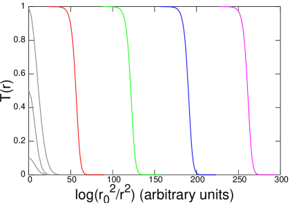
Figure 1: Picture of the evolution of $T(r)$ with rapidity (from left to right). Initially at $Y=0$, $T\sim T_{el}(r,r_{0})$. When rapidity increases, more dipoles populate the typical Fock state configuration, leading to a growing diffusion for $T$. Shortly after the unitarity limit $T=1$ is reached, a traveling wave forms.

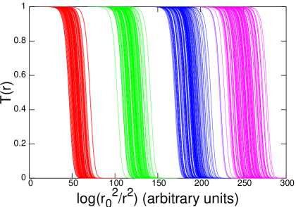
Figure 2: Different evolutions of a given initial condition over the rapidity ranges $Y_{0}$, $2Y_{0}$, $3Y_{0}$, $4Y_{0}$ (the bunches of curves gather 100 different realizations). One sees the dispersion of the front positions, which is of diffusive nature and thus of order $\Delta(\ln r_{0}^{2}Q_{s}^{2}(Y))\sim\sqrt{\bar{\alpha}Y}$.

3 Beyond the mean field: the “high energy QCD/sFKPP” correspondence

The mean field description outlined above is justified when the number of dipoles of a given size is large. However, in regions in which the amplitude $T$ is of order $\alpha_{s}^{2}$, the statistical fluctuations dominate and the mean field approximation breaks down. Both the fact that the number of dipoles of a given size is finite, and that this number fluctuates from event to event resulting in fluctuations $\delta T\sim\alpha_{s}\sqrt{T}$, are neglected in the mean field description (3). Since the tail $T\ll 1$ determines $Q_{s}$, we anticipate that these features have dramatic consequences. An evolution equation corrected for these effects may be written as

$$\partial_{\bar{\alpha}Y}T=\partial_{\rho}^{2}T+T-T^{2}+\alpha_{s}\sqrt{T(1-T)}\,\eta\ ,$$ (6)

where $\eta$ is a Gaussian white noise. With respect to Eq. (3), we have added a noise term that accounts for the statistical fluctuations in the dipole number. Eq. (6) is the stochastic Fisher-Kolmogorov (sFKPP) equation.

Significant progress has been achieved in the last few years in understanding the properties of its solutions [9]. It has been realized that the discreteness of the number of dipoles induces large corrections to the saturation scale, namely [9, 10, 3]

$$\ln r_{0}^{2}Q_{s}^{2}(Y)=\bar{\alpha}\frac{\chi(\gamma_{0})}{\gamma_{0}}Y-\bar{\alpha}\frac{\pi^{2}\gamma_{0}\chi^{\prime\prime}(\gamma_{0})}{2\ln^{2}1/\alpha_{s}^{2}}Y\ .$$ (7)

On the other hand, the fluctuations in the dipole number result in a diffusive wandering of the saturation scale: different events have saturation scales which typically differ by ${\cal O}(\sqrt{\bar{\alpha}Y}$). This is illustrated in Fig. 2 for a reaction-diffusion model that shares the essential properties of the full QCD problem (note that $\alpha_{s}=10^{-5}$, therefore statistical fluctuations in the tail are not distinguishable on the plot). After having averaged over many events to get the physical amplitude (2), the wandering of the saturation scale causes a drastic breaking of geometric scaling.

The variance of the wandering of the front has recently been quantified [9], and this result enables us to derive the scaling law for $A$ [3] that replaces geometric scaling (4):

$$A(Y,r)=A\left(\frac{\ln r^{2}Q_{s}^{2}(Y)}{\sqrt{\bar{\alpha}Y/\ln^{3}1/\alpha_{s}^{2}}}\right)\ .$$ (8)

Very recent work [11] has aimed at matching these ideas with the so-called Balitsky-Jalilian-Marian-Iancu-McLerran-Weigert-Leonidov-Kovner (JIMWLK) formulation of the color glass condensate [1], at the expense of a modification of the latter. We should stress that in any case, the results (7,8) directly stem from the physics of the parton model, and are presumably exact solutions of QCD: they are the leading terms in a large-$Y$ and small-$\alpha_{s}$ expansion.

References

- [1] For recent reviews and references, see e.g. R. Venugopalan, arXiv:hep-ph/0412396; H. Weigert, arXiv:hep-ph/0501087.
- [2] A. H. Mueller, Nucl. Phys. B 415 (1994) 373.
- [3] E. Iancu, A. H. Mueller and S. Munier, arXiv:hep-ph/0410018, Phys. Lett. B (2005).
- [4] I. Balitsky, Nucl. Phys. B 463 (1996) 99; Y.V. Kovchegov, Phys. Rev. D 60 (1999) 034008.
- [5] S. Munier and R. Peschanski, Phys. Rev. Lett. 91 (2003) 232001; Phys. Rev. D 69 (2004) 034008; Phys. Rev. D 70 (2004) 077503.
- [6] A. M. Stasto, K. Golec-Biernat and J. Kwiecinski, Phys. Rev. Lett. 86 (2001) 596.
- [7] L.V. Gribov, E.M. Levin and M. G. Ryskin, Phys. Rep. 100 (1983) 1.
- [8] A.H. Mueller and D. N. Triantafyllopoulos, Nucl. Phys. B 640 (2002) 331.
- [9] E. Brunet and B. Derrida, Phys. Rev. E 56 (1997) 2597; Comp. Phys. Comm. 121-122 (1999) 376; J. Stat. Phys. 103 (2001) 269.
- [10] A. H. Mueller and A. I. Shoshi, Nucl. Phys. B 692 (2004) 175.
- [11] E. Iancu and D. N. Triantafyllopoulos, arXiv:hep-ph/0411405; A. H. Mueller, A. I. Shoshi and S. M. H. Wong, arXiv:hep-ph/0501088.