A NEW OPTIMAL BOUND ON LOGARITHMIC SLOPE OF ELASTIC HADRON-HADRON SCATTERING

Abstract

In this paper we prove a new optimal bound on the logarithmic slope of the elastic slope b when: $\sigma_{el}$ and $\frac{d\sigma}{d\Omega}(1)$ and $\frac{d\sigma}{d\Omega}(-1),$ are known from experimental data. The results on the experimental tests of this new optimal bound are presented in Sect. 3 for the principal meson-nucleon elastic scatterings: ($\pi^{\pm}P\rightarrow\pi^{\pm}P$ and $K^{\pm}P\rightarrow K^{\pm}P)$ at all available energies. Then we show that the saturation of this optimal bound is observed with high accuracy practically at all available energies in meson-nucleon scattering.

1. Introduction

Recently, in Ref. [1], by using reproducing kernel Hilbert space (RKHS} methods [2-4], we described the quantum scattering of the spinless particles by a principle of minimum distance in the space of the scattering quantum states (PMD-SQS). Some preliminary experimental tests of the PMD-SQS, even in the crude form [1], when the complications due to the particle spins are neglected, showed that the actual experimental data for the differential cross sections of all $PP,$ $\overline{P}P,$ $K^{\pm}P,$ $\pi^{\pm}P,$ scatterings at all energies higher than 2 GeV, can be well systematized by PMD-SQS predictions. Moreover, connections between the optimal states [1], the PMD-SQS in the space of quantum states and the maximum entropy principle for the statistics of the scattering channels was also recently established by introducing quantum scattering entropies pl352 -prl83 .

The aim of this paper is to prove a new optimal bound on the logarithmic slope of the elastic hadron-hadron scattering by solving the following optimization problem: to find an lower bound on the logarithmic slope b when: $\sigma_{el}$, $\frac{d\sigma}{d\Omega}(+1)$ and $\frac{d\sigma}{d\Omega}(-1),$ including spin effects, are given. The results on the experimental tests of this new optimal bound are presented for the principal meson-nucleon elastic scatterings: ($\pi^{\pm}P\rightarrow\pi^{\pm}P$ and $K^{\pm}P\rightarrow K^{\pm}P)$ at all available energies. Then it was shown that the saturation of this optimal bound is observed with high accuracy practically at all available energies in meson-nucleon scattering.

2. Optimal helicity amplitudes for spin $(0^{-}1/2^{+}\rightarrow 0^{-}1/2^{+})$ scatterings

First we present some basic definitions and results for the optimal states in the meson-nucleon scattering when the integrated elastic cross section $\sigma_{el}$ and differential cross sections $\frac{d\sigma}{d\Omega}(\pm 1)$ are known from experiments. Therefore, let $f_{++}(x)$ and $f_{+-}(x)$, $x\in[-1,1]$, be the scattering helicity amplitudes of the meson-nucleon scattering process:

$$M(0^{-})+N(1/2^{+})\rightarrow M(0^{-})+N(1/2^{+})$$ (1)

$x=\cos\theta,\theta$ being the c.m. scattering angle. The formalizations of the helicity amplitudes $f_{++}(x)$ and $f_{+-}(x)$ are chosen such that the differential cross section $\frac{d\sigma}{d\Omega}(x)$ is given by

$$\frac{d\sigma}{d\Omega}(x)=\mid f_{++}(x)\mid^{2}+\mid f_{+-}(x)\mid^{2}$$ (2)

Then, the elastic integrated cross section $\sigma_{el}$ is given by

$$\frac{\sigma_{el}}{2\pi}=\int_{-1}^{+1}\frac{d\sigma}{d\Omega}(x)dx=\int_{-1}^{+1}[\mid f_{++}(x)\mid^{2}+\mid f_{+-}(x)\mid^{2}]dx$$ (3)

Since we will work at fixed energy, the dependence of $\sigma_{el}$ and,$\frac{d\sigma}{d\Omega}(x)$ and of $f(x)$, on this variable was suppressed. Hence, the helicities of incoming and outgoing nucleons are denoted by $\mu$, $\mu^{{}^{\prime}}$, and was written as (+),(-), corresponding to $(\frac{1}{2})$ and $(-\frac{1}{2})$, respectively. In terms of the partial waves amplitudes $f_{J+}$ and $f_{J-}$ we have

$$\left\{\begin{tabular}[]{l}$f_{++}(x)=\sum_{J=\frac{1}{2}}^{J_{\max}}(J+\frac{1}{2})(f_{J-}+f_{J+})d_{\frac{1}{2}\frac{1}{2}}^{J}(x)$\\ $f_{+-}(x)=\sum_{J=\frac{1}{2}}^{J_{\max}}(J+\frac{1}{2})(f_{J-}-f_{J+})d_{-\frac{1}{2}\frac{1}{2}}^{J}(x)$\end{tabular}\right\}$$ (4)

where the d${}_{\mu\nu}^{J}(x)$-rotation functions are given by

$$\left\{\begin{tabular}[]{l}$d_{\frac{1}{2}\frac{1}{2}}^{J}(x)=\frac{1}{l+1}\cdot\left[\frac{1+x}{2}\right]^{\frac{1}{2}}\left[P_{l+1}^{,}(x)-P_{l}^{,}(x)\right]$\\ $d_{-\frac{1}{2}\frac{1}{2}}^{J}(x)=\frac{1}{l+1}\cdot\left[\frac{1-x}{2}\right]^{\frac{1}{2}}\left[P_{l+1}^{,}(x)+P_{l}^{,}(x)\right]$\end{tabular}\right\}$$ (5)

and prime indicates differentiation of Legendre polinomials $P_{l}(x)$ with respect to x $\equiv\cos\theta$.

$$\frac{\sigma_{el}}{2\pi}=\sum(2J+1)\left[|f_{J^{+}}|^{2}+[f_{J^{-}}|^{2}\right]$$ (6)

Now, let us consider the optimization problem

$$\left\{\begin{tabular}[]{l}$\min\left[\sum(2J+1)(|f_{J^{+}}|^{2}+|f_{J-}|^{2})\right],$ $\text{subject to: }$\\ $\frac{d\sigma}{d\Omega}(+1)=fixed,$and $\frac{d\sigma}{d\Omega}(-1)=fixed$\end{tabular}\right\}$$ (7)

which will be solved by using Lagrange multiplier method [9] where

$$\left\{\begin{tabular}[]{l}$\pounds=\left[\sum(2J+1)(|f_{J^{+}}|^{2}+|f_{J-}|^{2})\right]$\\ $+\alpha\left[\frac{d\sigma}{d\Omega}(+1)-|\sum(J+1/2)(f_{J-}+f_{J+})|^{2}\right]$\\ $+\beta\left[\frac{d\sigma}{d\Omega}(-1)-|\sum(J+1/2)(f_{J-}-f_{J+})|^{2}\right]$\end{tabular}\right\}$$ (8)

So, we prove that the solution of the problem (7)- (8) is as follows

$$\left\{\begin{tabular}[]{l}$f_{++}^{o}(x)=f_{++}(+1)\cdot\frac{K_{\frac{1}{2}\frac{1}{2}}(x,+1)}{K_{\frac{1}{2}\frac{1}{2}}(+1,+1)}$\\ $f_{+-}^{o}(x)=f_{+-}(-1)\cdot\frac{K_{-\frac{1}{2}\frac{1}{2}}(x,-1)}{K_{-\frac{1}{2}\frac{1}{2}}(-1,-1)}$\end{tabular}\right\}$$ (9)

where the reproducing kernel functions are defined as

$$\left\{\begin{tabular}[]{l}$K_{\frac{1}{2}\frac{1}{2}}(x,y)=\sum_{\frac{1}{2}}^{J_{o}}(J+\frac{1}{2})d_{\frac{1}{2}\frac{1}{2}}^{J}(x)d_{\frac{1}{2}\frac{1}{2}}^{J}(y)$\\ $K_{-\frac{1}{2}\frac{1}{2}}(x,y)=\sum_{\frac{1}{2}}^{J_{o}}(J+\frac{1}{2})d_{-\frac{1}{2}\frac{1}{2}}^{J}(x)d_{-\frac{1}{2}\frac{1}{2}}^{J}(y)$\\ \begin{tabular}[]{l}$2K_{\frac{1}{2}\frac{1}{2}}(+1,+1)=(J_{o}+1)^{2}-1/4$\\ $2K_{-\frac{1}{2}\frac{1}{2}}(-1,-1)=(J_{o}+1)^{2}-1/4$\end{tabular}\\ $(J_{o}+1)^{2}-\frac{1}{4}=\frac{4\pi}{\sigma_{el}}\cdot\left[\frac{d\sigma}{d\Omega}(1)+\frac{d\sigma}{d\Omega}(-1)\right]$\end{tabular}\right\}$$ (10)

Proof: Let us consider the complex partial amplitudes $f_{J^{\pm}}\equiv r_{J^{\pm}}+ia_{J^{\pm}},$where $r_{J^{\pm}}$ and $a_{J^{\pm}}$ are real and imaginary parts, respectively. Then, Eq.(8) can be expressed completely in terms of the variational variables $r_{J^{\pm}}$ and $a_{J^{\pm}}$. Therefore, by calculating the first derivative we obtain

$$\left\{\begin{tabular}[]{l}$\frac{1}{(2J+1)}\frac{\partial\pounds}{\partial r_{J^{\pm}}}=r_{J^{\pm}}-\alpha R^{++}(+1)\pm\beta R^{+-}(-1)=0$\\ $\frac{1}{(2J+1)}\frac{\partial\pounds}{\partial a_{J^{\pm}}}=a_{J^{\pm}}-\alpha A^{++}(+1)\pm\beta A^{+-}(-1)=0$\end{tabular}\right\}$$ (11)

where we have defined $f^{++}(x)\equiv R^{++}(x)+iA^{++}(x),$ and $f^{+-}(x)\equiv R^{+-}(x)+iA^{+-}(x)$, respectively, where

$$R^{++}(+1)=\sum(J+\frac{1}{2})(r_{J^{+}}+r_{J^{-}})$$

(12)

Therefore, from Eqs (11) we get

$$\left\{\begin{tabular}[]{l}$r_{J+}=\alpha R^{++}(+1)-\beta R^{+-}(-1)$\\ $r_{J-}=\alpha R^{++}(+1)+\beta R^{+-}(-1)$\\ $a_{J+}=\alpha A^{++}(+1)-\beta A^{+-}(-1)$\\ $a_{J^{-}}=\alpha A^{++}(+1)+\beta A^{+-}(-1)$\end{tabular}\right\}$$ (13)

Then, using the definitions (2) and (3), we get

$$\alpha^{-1}=\beta^{-1}=(J_{o}+1)^{2}-1/4=\frac{4\pi}{\sigma_{el}}\left[\frac{d\sigma}{d\Omega}(+1)+\frac{d\sigma}{d\Omega}(-1)\right]$$ (14)

and, consequently we obtain that the optimal solution of the problem (7) can be written in the form

$$f_{++}^{o}(x)=\frac{2f_{++}(+1)}{(J_{o}+1)^{2}-1/4}\sum_{1/2}^{J_{o}}(J+\frac{1}{2})d_{\frac{1}{2}\frac{1}{2}}^{J}(x)d_{\frac{1}{2}\frac{1}{2}}^{J}(+1)$$

(15)

Now from Eqs. (14) and (15) we obtain the optimal solution (9) in which the reproducing functions $K_{\frac{1}{2}\frac{1}{2}}(x,y)$ and $K_{-\frac{1}{2}\frac{1}{2}}(x,y)$ are defined by (10).

3. Optimal bound on logarithmic slope

We recall the definition of the elastic slope b, and the relation

$$b\equiv\frac{d}{dt}\left[\ln\frac{d\sigma}{dt}(s,t)\right]|_{t=0}=\frac{\overline{\lambda}^{2}}{2}\frac{d}{dx}\left[\ln\frac{d\sigma}{d\Omega}(x)\right]|_{x=1}$$ (16)

where transfer momentum is defined by : $t=-2q^{2}(1-x),$ $\overline{\lambda}=1/q,$and $q$ is the c.m momentum.

Now, let us assume that $\sigma_{el}$, $\frac{d\sigma}{d\Omega}(+1),$ and $\frac{d\sigma}{d\Omega}(-1)$ are known from the experimental data. Then, taking into account the solution (9)-(10) of the optimization problem (7), it is easy to prove that the elastic slope b defined by (16) must obey the optimal inequality:

$$b\geq b_{o}\equiv\frac{\overline{\lambda}^{2}}{4}\left\{\frac{4\pi}{\sigma_{el}}\cdot\left[\frac{d\sigma}{d\Omega}(+1)+\frac{d\sigma}{d\Omega}(-1)\right]-1\right\}$$ (17)

Proof: Indeed a proof of the optimal inequality (17) can be obtained as singular solution of the following optimization problem

$$\min\left\{b\right\},\text{ subject to: }\sigma_{el}=\text{fixed, }$$

(18)

So, the lower limit of the elastic slope b is just the elastic of the differential cross section given by the result (9)-(10). Consequently, we obtain that the optimal slope $b_{o}$ is given by

$$b_{o}=\overline{\lambda}^{2}\frac{d}{dx}\left[\frac{K_{\frac{1}{2}\frac{1}{2}}(x,+1)}{K_{\frac{1}{2}\frac{1}{2}}(+1,+1)}\right]|_{x=1}=\frac{\overline{\lambda}^{2}}{4}\left\{\left[J_{o}(J_{o}+2)-\frac{1}{4}\right]\right\}$$ (19)

Then, using the second part of (14) we obtain the inequality (17).

An important model independent result obtained Ref. [1], via the description of quantum  scattering by the principle of minimum distance in space of states (PMD-SS), is the following optimal lower bound on logarithmic slope of the forward diffraction peak in hadron-hadron elastic scattering:

$$b\geq b_{o}\geq\frac{\overline{\lambda}^{2}}{4}\left[\frac{4\pi}{\sigma_{el}}\frac{d\sigma}{d\Omega}(1)-1\right]$$ (20)

In is important to remark, the optimal bound (17) improves in a more general and exact form not only the unitarity bounds derived by MacDowell and Martin McDow for the logarithmic slope $b_{A}$ of absorptive contribution $\frac{d\sigma_{A}}{d\Omega}(s,t)$ to the elastic differential cross sections but also the unitarity lower bound derived in Ref. [1] (see also Ref. scf , rjf49 ) for the slope $b$ of the entire $\frac{d\sigma}{d\Omega}(s,t)$ differential cross section. Therefore, it would be important to make an experimental detailed investigation of the saturation of this bond in the hadron-hadron scattering, especially in the low energy region.

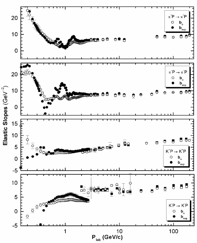
4. Experimental tests of the bound (17)

A comparison of the experimental elastic slopes b with the optimal slope $b_{o}(17)$ is presented in Figs. 1 for ($\pi^{\pm}P$ and $K^{\pm}P)$-scatterings: The values of the $\chi^{2}=\sum_{j}(b_{j}-b_{oj})^{2}/(\epsilon_{bj}^{2}+\epsilon_{b_{o}j}^{2})$, (where $\epsilon_{bj}$ and $\epsilon_{b_{o}j}$ are the experimental errors corresponding to $b$ and $b_{o}$ respectively) are used for the estimation of departure from the optimal PMD-SS-slope $b_{o}$, and then, we obtain the statistical parameters presented in Table 1. For $\pi^{\pm}P$-scattering the experimental data on $b$, $\frac{d\sigma}{d\Omega}(+1),$ $\frac{d\sigma}{d\Omega}(-1),$and $\sigma_{el}$ , for the laboratory momenta in the interval $0.2$ GeV$\leq p_{LAB}\leq 10$ $GeV$ are calculated directly from the phase shifts analysis (PSA) of Hohler et al. hohler . To these data we added some values of $b$ from the linear fit of Lasinski et al. lasinski and also from the original fit of authors quoted in some references in rjf49 . Unfortunately, the values of $b_{o}$ corresponding to the Lasinski’s data lasinski was impossible to be calculated since the values of $\frac{d\sigma}{d\Omega}(1)$ from their original fit are not given. For $K^{\pm}P-$scatterings the experimental data on $b$, $\frac{d\sigma}{d\Omega}(+1),$ $\frac{d\sigma}{d\Omega}(-1)$ and $\sigma_{el}$ , in the case of $K^{-}P$, are calculated from the experimental (PSA) solutions of Arndt et al. arndt . To these data we added those collected from the original fit of data from references of rjf49 which the approximation $\frac{d\sigma}{d\Omega}(-1)=0$. For $K^{+}P$-scattering, we added some values of $b$ from the linear fit of Lasinski et al. lasinski and also those pairs $(b,b_{o})$ calculated directly from the experimental (PSA) solutions of Arndt et al. arndt . All these results can be compared with those presented in Ref. rjf49 .

5. Summary and Conclusion

The main results and conclusions obtained in this paper can be summarized as follows:

(i) In this paper we proved the optimal bound (17) as the singular solution ($\lambda_{0}=0)$ of the optimization problem to find a lower bound on the logarithmic slope b with the constraints imposed when $\sigma_{el}$ and $\frac{d\sigma}{d\Omega}(+1)$ and $\frac{d\sigma}{d\Omega}(-1)$ are fixed from experimental data. This result is similar with that obtained recently in Refs. 1 , rjf49 for the problem to find an upper bound for the scattering entropies when $\sigma_{el}$ and $\frac{d\sigma}{d\Omega}(+1)$ are fixed.

(ii) We find that the optimal bound (17) is verified experimentally with high accuracy at all available energies for all the principal meson-nucleon scatterings.

(iii). From mathematical point of view, the PMD-SQS-optimal states (9)-(10), are functions of minimum constrained norm and consequently can be completely described by reproducing kernel functions (see also Ref. [1,3-4].  So, with this respect the PMD-SQS-optimal states from the reproducing kernel Hilbert space (RKHS) of the scattering amplitudes are analogous to the coherent states from the RKHS of the wave functions.

(iv) The PMD-SQS-optimal state (9)-(10) have not only the property that is the most forward-peaked quantum state but also possesses many other peculiar properties such as maximum Tsallis-like entropies, as well as the scaling and the s-channel helicity conservation properties, etc., that make it a good candidate for the description of the quantum scattering.via an optimum principle. In fact the validity of the principle of least distance in space of states in hadron-hadron scattering is already well illustrated in Fig. 1 and Table 1.

All these important properties of the optimal helicity amplitudes (9)-(10) will be discussed in more detail in a forthcoming paper.

Table 1: $\stackrel{{\scriptstyle\_}}{{\chi^{2}}}-$statistical parameters of the principal hadron-hadron scattering. In these estimations for P${}_{LAB}\leq 2$ GeV/c the errors $\epsilon_{b}^{PSA}(\pi^{\pm}P)=0.1$ $b^{PSA}$ and $\epsilon_{b_{o}}^{PSA}(K^{\pm}P)=0.1b^{PSA}$ are taken into account while for the errors to the optimal slopes b_o calculated from phase shifts analysis and rjf49 .

		For P${}_{LAB}\geq 2GeV/c$		For all P${}_{LAB}\geq 0.2GeV/c$
Statistical parameters	Np	$\quad\,\quad\quad\chi^{2}/$ndof	Np	$\quad\quad\chi^{2}/$ndof
$\quad\pi^{+}P\rightarrow\pi^{+}P$	28	1.02	90	3.37
$\quad\pi^{-}P\rightarrow\pi^{-}P$	31	0.92	93	8.00
$\quad K^{+}P\rightarrow K^{+}P$	37	1.15	73	1.91
$\quad K^{-}P\rightarrow K^{-}P$	37	1.52	73	7.84
$\quad PP\rightarrow PP$	29	5.01	32	5.06
$\quad\bar{P}P\rightarrow\bar{P}P$	27	0.56	45	1.86

Figure 1: The experimental values (black circles) of the logarithmic slope b for the principal meson-nucleon scatterings are compared with the optimal PMD-SQS-predictions $b_{o}$ (white circles). The experimental data for $b$, $\frac{d\sigma}{d\Omega}(+1)$ and $\sigma_{el}$, are taken from Refs. hohler -lasinski . (see the text).

References

• (1) D. B. Ion, Phys. Lett. B 376, 282 (1996), and quoted therein references.
• (2) N. Aronsjain, Proc. Cambridge Philos. Soc. 39 (1943) 133, Trans. Amer. Math. Soc. 68 (1950) 337; A. Meschkowski, Hilbertische Raume mit Kernfunction, Springer Berlin, 1962.
• (3) D.B.Ion and H.Scutaru, International J.Theor.Phys. 24, 355 (1985);
• (4) D.B.Ion, International J.Theor.Phys. 24, 1217 (1985) ; D.B.Ion, International J.Theor.Phys. 25, 1257 (1986).
• (5) D. B. Ion, M. L. Ion, Phys. Lett. B 352, 155 (1995),
• (6) D. B. Ion, M. L. Ion, Phys. Lett. B 379, 225 (1996).
• (7) D. B. Ion, M. L. D. Ion, Phys. Rev. Lett. 81, 5714 (1998).
• (8) M. L. D. Ion, D. B. Ion, Phys. Rev. Lett. 83, 463 (1999); D. B. Ion, M. L. D. Ion, Phys. Rev. E 60, 5261 (1999); M. L. D. Ion, D. B. Ion, Phys. Lett. B 482, 57 (2000); D. B. Ion, M. L. D. Ion, Phys. Lett. B 503, 263 (2001); D. B. Ion, M. L. D. Ion, Phys. Lett. B 519, 63 (2001); D. B. Ion, M. L. D. Ion, Chaos Solitons and Fractals,13, 547 (2002).
• (9) M. B. Einhorn and R. Blankenbecler, Ann. of Phys. (N. Y.), 67, 480 (1971).
• (10) S. W. MacDowell, A. Martin, Phys. Rev. 135B, 960 (1964).
• (11) D. B. Ion, St. Cerc. Fiz. 43, 5 (1991).
• (12) G. Hohler, F. Kaiser, R. Koch, E. Pitarinen, Physics Data, Handbook of Pion Nucleon Scattering, 1979, Nr. 12-1.
• (13) R. A. Arndt and L. D. Roper, Phys. Rev. D31, 2230 (1985).
• (14) T. Lasinski, R. Seti, B. Schwarzschild and P. Ukleja, Nucl. Phys. B37, 1 (1972).
• (15) See the complete list of references in: D. B. Ion, M. L. Ion, Rom. J. Phys. 49, Nr. 7-8 (2004) . e-Print archive hep-ph/0302018.