UH-511-1066-05 Fully differential Higgs boson production and the di-photon signal through next-to-next-to-leading order

Abstract

We describe a calculation of the fully differential cross section for Higgs boson production in the gluon fusion channel through next-to-next-to-leading order (NNLO) in perturbative QCD. The decay of the Higgs boson into two photons is included. Technical aspects of the computation are discussed in detail. The implementation of the calculation into a numerical code, called  FEHiP, is described. The NNLO $K$-factors for completely realistic photon acceptances and isolation cuts, including those employed by the ATLAS and CMS collaborations, are computed. We study various distributions of the photons from Higgs decay through NNLO.

I Introduction

Perturbative calculations in quantum field theory have been performed since the birth of QED in the 1930s. Enormous progress has been made since this early era, and the tools used to obtain these results have improved dramatically. Much of this progress has been spurred by the constantly increasing demands of the high energy experimental program. Future experiments such as the LHC and the Next Linear Collider are now demanding perturbative calculations to next-to-next-to-leading order (NNLO) in the relevant coupling constants. These results must also be directly applicable to experimental measurements, which requires calculational algorithms flexible enough to allow arbitrary constraints on the final state of reactions.

For a long time, virtual corrections hindered the progress of perturbative calculations. With the advent of computer algebra and the realization that loop integrals satisfy simple identities that follow from their generalized hypergeometric nature tkachov , virtual corrections for processes with a small number of kinematic invariants became relatively straightforward loop1 ; loop2 ; loop3 ; laporta . However, physical results require the inclusion of real emission corrections, in which additional massless partons are emitted into the final state. It was recognized early in the history of perturbative calculations, first in QED and then in QCD, that such emissions lead to infrared and collinear singularities when the initial or final state configurations become degenerate. The Bloch-Nordsieck and Kinoshita-Lee-Nauenberg theorems Bloch:1937pw ; Kinoshita:1962ur ; Lee:1964is show that both virtual corrections and real emissions must be included to obtain a physically meaningful result, because divergences only cancel when these components are combined. The methods cited above rely upon special features of loop integrals. They can be used to obtain virtual corrections, or inclusive cross sections related to virtual corrections through the optical theorem, such as the total hadroproduction cross section in $e^{+}e^{-}$ collisions. Recently, these methods have also been extended to phase-space integrals for total cross sections and simple kinematic distributions Anastasiou:2002yz ; Anastasiou:2002wq ; Anastasiou:2002qz ; Anastasiou:2003yy ; Anastasiou:2003ds ; Melnikov:2004bm ; Mitov:2004du . However, observables where the phase space is non-trivially constrained cannot be obtained using these techniques. Unfortunately, these are exactly the quantities required by experiment; because of final-state cuts, inclusive results are of limited use.

Virtual corrections possess a simple mathematical structure, and the extraction of their singularities proceeds in an observable-independent fashion. With real corrections, different kinematic cuts are imposed on the final state for different observables. Since we would like to perform calculations valid for arbitrary cuts, the extraction of singularities from real emission corrections should be performed in the presence of an unspecified “measurement function”. The factorization of soft and collinear emissions renders such an extraction possible. The resulting cancellation of singularities requires that the measurement function allows only “infrared safe” observables that can be computed in perturbation theory sterman .

An efficient algorithm for extracting singularities at NLO in perturbative QCD was constructed in Catani:1996vz ; Catani:2002hc , advancing earlier work on the subject nloreal . This “dipole-subtraction” algorithm identifies universal soft and collinear counterterms, called dipoles, that can be subtracted from the real emission contribution to an arbitrary process to make it finite. The dipoles can then be analytically integrated over the restricted phase space, since the measurement function for infrared safe observables collapses to a measurement function of lower multiplicity in the soft and collinear limits. After integration, the dipoles cancel the infrared divergences in the virtual corrections, leading to a finite result.

For processes where the perturbative corrections are large, or control of the theoretical error is crucial, perturbative calculations must be extended to NNLO. Either an extension of the dipole formalism to NNLO or the development of an alternative approach is needed to enable these computations. Significant effort has been devoted to a generalization of the dipole subtraction method Kosower:2002su ; Kosower:2003cz ; Weinzierl:2003fx ; Weinzierl:2003ra ; Gehrmann-DeRidder:2004tv ; Gehrmann-DeRidder:2003bm ; Gehrmann-DeRidder:2004xe ; Kilgore:2004ty ; Frixione:2004is . This extension has remained elusive. Although the infrared behavior of loop amplitudes catani ; tejeda and the infrared limits of real emission corrections are universal at NNLO amplfactor , it becomes much more difficult to disentangle the singularities of two unresolved emissions, and to construct process-independent counterterms.

We have recently developed an alternative approach to the problem of real radiation at NNLO sector . Our method differs conceptually from the dipole subtraction approach in two important ways: the finding of singular phase-space regions is completely automated; the cancellation of the $1/\epsilon$ poles which describe divergences in dimensional regularization is performed numerically, and no analytic integrations are required. These features guarantee that it can be used to extract and cancel singularities at any order in perturbation theory, at least in principle. The primary complication that occurs at higher orders is the presence of overlapping singularities. These can be disentangled using sector decomposition Binoth:2000ps ; hepp ; Roth:1996pd . Existing symbolic manipulation programs, such as MAPLE or MATHEMATICA, provide a suitable framework in which to program the algorithm. The extraction and cancellation of singularities is thus achieved in a completely automated fashion, with little human intervention.

We have used this approach to perform two fully differential calculations through NNLO in QCD: the ${\cal O}(\alpha_{s}^{2})$ correction to $e^{+}e^{-}\to 2~{}{\rm jets}$ sector ; Anastasiou:2004qd , and the Higgs boson hadroproduction cross section through gluon fusion higgsdiff . Both calculations permit arbitrary cuts on the final states and can easily be extended to include decays of the final state particles. These successful applications demonstrate the vitality of our approach and its potential relevance for other problems of phenomenological importance; we therefore believe it is important to describe it in a simple, pedagogical fashion. We attempt to do so in this manuscript. Our discussion will be centered around the calculation of the Higgs hadroproduction cross section completed recently higgsdiff . We will extend this result to include the decay of the Higgs through the channel $H\rightarrow\gamma\gamma$. We therefore pursue two goals in this paper: a thorough discussion of the analytic aspects of our calculation and its implementation into a numerical code, and a presentation of phenomenological results for $pp\rightarrow H+X\rightarrow\gamma\gamma+X$ through NNLO in QCD.

This paper is organized as follows. In the next Section we describe phenomenological issues relevant for Higgs boson hadroproduction. In Section III we introduce our notation, and describe the basic setup of our calculation. In Section IV we discuss Higgs production in association with up to one parton. Section V is devoted to the calculation of the collinear counterterms. The phase-space parameterization is a crucial element of our approach; we describe details regarding the choice of parameterizations for Higgs hadroproduction in Section VI. We discuss how to handle the various forms of singularities which appear in NNLO computations in the following Section. In Section VIII we discuss how the matrix elements that appear in the double real emission contribution for Higgs hadroproduction are treated in our calculation. We then present phenomenological results for $pp\rightarrow H+X$ and $pp\rightarrow H+X\rightarrow\gamma\gamma+X$ through NNLO in perturbative QCD. We next describe the implementation of our results into the numerical code  FEHiP. We conclude with a discussion of the advantages and disadvantages of our approach, and identify directions for future work.

II Higgs boson production at hadron colliders

We describe here the aspects of Higgs phenomenology at the LHC needed for our calculation. There are several mechanisms for Higgs production at hadron colliders (see Carena:2002es for a review). For most Higgs masses, gluon fusion through a top quark loop, $gg\to H$, is the dominant production mechanism. For Higgs masses in the range preferred by the global fit to the precision electroweak data ewkprecision , $m_{h}\approx 110-130$ GeV, the gluon fusion cross section is approximately $60~{}{\rm pb}$. The Higgs branching fraction into two photons is larger than $10^{-3}$ in this mass range prod ; dec . The search strategy search for the Higgs signal is then to look for events with two isolated photons and reconstruct the mass of the Higgs boson by studying their invariant mass distribution. The photons are required to have transverse momenta $p_{\bot}^{(1)}\geq 40~{}{\rm GeV}$ and $p_{\bot}^{(2)}\geq 25~{}{\rm GeV}$; they must also be produced in the central rapidity region $|\eta|<2.5$ search . The major irreducible background to two photon events is direct (prompt) di-photon production in hadronic collisions diphot ; a $1\%$ photon energy resolution is needed to distinguish the $H\to\gamma\gamma$ signal over the background. Typically, an isolation cut is also imposed upon the photons; this suppresses photons from the decays of large $p_{\bot}$ hadrons, such as $\pi^{0}\to\gamma\gamma$, and from the poorly known fragmentation production of prompt photons. Several possible isolation cuts have been proposed lance1 ; smoothcone ; difox ; search . The simplest possibility is to require that a photon candidate does not have additional transverse energy $E_{\rm T,min}$ deposited within the region $R_{\rm is}=\sqrt{(\eta-\eta_{\gamma})^{2}+(\phi-\phi_{\gamma})^{2}}$ in the $(\eta,\phi)$ plane. Typical values used in previous studies are $E_{\rm T,min}=4-15~{}{\rm GeV}$ and $R_{\rm is}=0.4$.

The Higgs production cross section receives large perturbative corrections and depends strongly on the renormalization and factorization scales. For example, for $m_{h}=100-130~{}{\rm GeV}$, the cross section for $pp\to H+X$ at $\sqrt{s}=14~{}{\rm TeV}$ increases by a factor $1.5-1.7$ when the NLO QCD corrections are included dawson ; spira . The residual scale dependence at NLO is approximately thirty percent. This peculiar behavior of the perturbative series motivated several NNLO calculations of the inclusive Higgs production cross section Harlander:2001is ; Harlander:2002wh ; Catani:2001ic ; Anastasiou:2002yz ; Ravindran:2003um . These studies found no breakdown of the perturbative expansion; while the NNLO effects are sizable, they are smaller than the NLO ones. The NNLO cross section is also much more stable against variations of the renormalization and the factorization scales. These results were confirmed Catani:2003zt in the framework of threshold resummation, which exploits the fact that because of the large value of the gluon density at small Bjorken $x$, the Higgs production cross section at the LHC is dominated by the partonic threshold, i.e., the $z\to 1$ region, where $z=m_{h}^{2}/s_{\rm part}$. The terms that are singular in this limit can be systematically resummed to all orders in $\alpha_{s}$, and the results compared to the complete NNLO calculation. The two approaches agree well, indicating that the uncalculated higher order effects are likely to be within the uncertainty assigned to the NNLO result.

Much is also known about less inclusive quantities for Higgs boson production. The NLO $p_{\bot}$ and rapidity distributions for Higgs boson production at high $p_{\bot}$ are computed in Ravindran:2002dc . In addition, the rapidity distribution of the Higgs boson has been computed through NLO Anastasiou:2002qz ; lance1 . The $p_{\bot}$ distribution of the Higgs boson has been investigated using various resummation formalisms by different groups group1 ; group2 ; group3 ; group4 . Monte Carlo event generators accurate through NLO for the ${\rm Higgs}+{\rm jet}$ process have been published deFlorian:1999zd ; Campbell:2000bg . Higgs production is also included in existing shower Monte Carlo event generators, such as PYTHIA and HERWIG, and in the MC@NLO event generator that correctly combines single hard gluon emissions with the HERWIG parton shower mcatnlo . The di-photon invariant mass distribution in $pp$ collisions, including both the signal $pp\to H+X\to\gamma\gamma+X$ and the prompt photon background $pp\to\gamma\gamma$, can be found in difox ; lance1 ; lance2 . Ref. difox presents the partonic level event generator DIPHOX, where both direct and fragmentation components of the prompt photon production are computed through NLO in perturbative QCD. In lance1 , the QCD corrections to the $gg\to\gamma\gamma$ channel of diphoton production are computed; combined with DIPHOX, this presents the most up-to-date analysis of the two photon background to Higgs production and enables a careful analysis of the signal-to-background ratio as a function of the isolation cuts. In lance2 , the interference between the signal and background is shown to be negligible.

Clearly, a substantial amount is known about Higgs hadroproduction; unfortunately, only the inclusive cross section is known through NNLO. Since the NNLO corrections are large, it is desirable to also know differential quantities to this order. This is necessary to compute the $K$-factor, $K_{\rm NNLO}=\sigma_{\rm NNLO}/\sigma_{\rm LO}$, that corresponds to realistic experimental acceptances with cuts on the photons and jets in the final state. Although the kinematics of the $H\rightarrow\gamma\gamma$ decay is not altered by higher order QCD effects, the QCD corrections to the production process change the kinematics of the produced Higgs boson and lead to modifications in the kinematics of the produced photons. In order to compute the relevant acceptance through NNLO, the Higgs boson production cross section must be known at the differential level. We begin our description of this calculation in the following Section.

III Notation and Setup

We study the production of a Higgs boson with momentum $p_{h}$ in the collision of two hadrons, $h_{1}$, $h_{2}$, carrying momenta $P_{1},P_{2}$:

$$h_{1}(P_{1})+h_{2}(P_{2})\to H(p_{h})+X.$$ (1)

Within the framework of QCD factorization, the cross section for this process can be written as an integral over hard scattering cross sections $\sigma_{ij}$ for the production of the Higgs boson from the quarks and gluons, multiplied by parton densities describing the distribution of these partons inside the colliding hadrons:

$$\sigma=\sum_{ij}\int_{0}^{1}dx_{1}dx_{2}f_{i}^{\left(h_{1}\right)}(x_{1})f_{j}^{\left(h_{2}\right)}(x_{2})\sigma_{ij\to H+X}(x_{1},x_{2}).$$ (2)

The sum is over the parton flavors $i,j$ in the hadrons $h_{1},h_{2}$, and $f_{i}^{(h_{1})},f_{j}^{(h_{2})}$ are the corresponding parton densities. The initial-state partons $i,j$ for the hard scattering partonic process carry momenta $p_{1}=x_{1}P_{1}$ and $p_{2}=x_{2}P_{2}$. The partonic cross sections for the processes $i+j\to H+X$, can be calculated perturbatively; here, we compute them through ${\cal O}(\alpha_{s}^{4})$ in the strong coupling expansion:

$$\sigma_{ij\to H+X}=\alpha_{s}^{2}\left[\sigma_{ij}^{(0)}+\frac{\alpha_{s}}{\pi}\sigma_{ij}^{(1)}+\left(\frac{\alpha_{s}}{\pi}\right)^{2}\sigma_{ij}^{(2)}\right]+{\cal O}(\alpha_{s}^{5}).$$ (3)

The partonic cross sections $\sigma_{ij}$ contain divergences arising from intial-state collinear radiation; these are removed by recasting the parton-densities in the $\overline{\rm MS}$-factorization scheme. The hadronic cross section of Eq. 2 is computed in terms of finite parton densities $\tilde{f}$ and finite partonic cross sections $\hat{\sigma}$,

$$\sigma=\sum_{ij}\int_{0}^{1}dx_{1}dx_{2}\tilde{f}_{i}^{\left(h_{1}\right)}(x_{1})\tilde{f}_{j}^{\left(h_{2}\right)}(x_{2}){\hat{\sigma}}_{ij\to H+X}(x_{1},x_{2}).$$ (4)

The finite and “bare” parton densities are related via

$$\tilde{f}_{i}^{(h)}=\sum_{j}f_{j}^{(h)}\otimes\Gamma_{ij},$$ (5)

where we have introduced the convolution integral

$$(f\otimes g)(x)=\int_{0}^{1}dydzf(y)g(z)\delta(x-yz).$$ (6)

The functions $\Gamma_{ij}$ are given in the $\overline{{\rm MS}}$ scheme by

$$\Gamma_{ij}(x) = \delta_{ij}\delta(1-x)-\frac{\alpha_{s}}{\pi}\frac{P_{ij}^{(0)}}{\epsilon}$$ (7)

$$+\left(\frac{\alpha_{s}}{\pi}\right)^{2}\left\{\frac{1}{2\epsilon^{2}}\left[\sum_{k}\left(P_{ik}^{(0)}\otimes P_{kj}^{(0)}\right)(x)+\beta_{0}P_{ij}^{(0)}\right]-\frac{1}{2\epsilon}P_{ij}^{(1)}(x)\right\}+{\cal O}\left(\alpha_{s}^{3}\right)$$

where the Altarelli-Parisi kernels $P_{ij}^{(n)}$ can be found in splitting1 ; splitting2 . We note that the complete NNLO corrections to these kernels have recently been computed splitting3 . $\epsilon=(4-d)/2$ is the usual dimensional regularization parameter; all calculations in this paper are performed using this regularization scheme. Substituting Eq. (6) into Eq. (4) and comparing with Eq. (2) we find

$$\sigma_{ij}=\sum_{kl}\int_{0}^{1}dy_{1}dy_{2}\Gamma_{ik}(y_{1})\Gamma_{jl}(y_{2})\hat{\sigma}_{kl}(x_{1}y_{1},x_{2}y_{2}).$$ (8)

We compute the finite partonic cross sections $\hat{\sigma}_{ij}$ by expanding

$$\hat{\sigma}_{ij}=\alpha_{s}^{2}\left[\hat{\sigma}_{ij}^{(0)}+\frac{\alpha_{s}}{\pi}\hat{\sigma}_{ij}^{(1)}+\left(\frac{\alpha_{s}}{\pi}\right)^{2}\hat{\sigma}_{ij}^{(2)}\right]+{\cal O}(\alpha_{s}^{5}),$$ (9)

and solving Eq. (8) in terms of the coefficients $\hat{\sigma}_{ij}^{(n)}$ order-by-order in the strong coupling expansion. In this procedure, we need to consider the convolution integrals of the partonic cross sections with the Altarelli-Parisi kernels at each order in the perturbative expansion; this will be discussed in detail in a later Section.

We now discuss the Lagrangian which describes Higgs boson production. As mentioned in the previous Section, we consider the gluon fusion mechanism for Higgs production. The Higgs coupling to two gluons is induced by a top quark loop prod ; if there are other heavy quark doublets that acquire mass from the Higgs mechanism, they might also give a substantial contribution to the effective $Hgg$ coupling. We focus here on a light Standard Model Higgs boson whose mass is smaller than twice the mass of the top quark: $m_{h}\leq 2m_{t}\approx 350~{}{\rm GeV}$. The interaction of the Higgs boson with two gluons can then be described by a point-like vertex prod ; this is formalized by introducing the effective Lagrangian

$${\cal L}=\frac{1}{4v}C_{1}Z_{1}G^{a}_{\mu\nu}G^{a\mu\nu}H,$$ (10)

where $G^{a}_{\mu\nu}$ is the gluon field strength tensor, $H$ is the Higgs field, and $v\simeq 246$ GeV is the Higgs boson vacuum expectation value. The Wilson coefficient $C_{1}$ and the renormalization factor $Z_{1}$, defined in the $\overline{{\rm MS}}$ scheme, are koeffc1

$$C_{1}=-\frac{1}{3\pi}\left\{1+\frac{11}{4}\frac{\alpha_{s}}{\pi}+\left(\frac{\alpha_{s}}{\pi}\right)^{2}\left[\frac{2777}{288}+\frac{19}{16}L_{t}+n_{f}\left(-\frac{67}{96}+\frac{1}{3}L_{t}\right)\right]+{\cal O}\left(\alpha_{s}^{3}\right)\right\},$$

$$Z_{1}=1-\frac{\alpha_{s}}{\pi}\frac{\beta_{0}}{\epsilon}+\left(\frac{\alpha_{s}}{\pi}\right)^{2}\left[\frac{\beta_{0}^{2}}{\epsilon^{2}}-\frac{\beta_{1}}{\epsilon}\right]+{\cal O}\left(\alpha_{s}^{3}\right),$$ (11)

where $\alpha_{s}=\alpha_{s}(\mu)$ is the QCD $\overline{{\rm MS}}$ coupling constant, defined in the theory with $n_{f}=5$ flavors, and

$$L_{t}=\log\left(\frac{\mu^{2}}{m_{top}^{2}}\right),\quad\beta_{0}=\frac{11}{4}-\frac{n_{f}}{6},\quad\beta_{1}=\frac{51}{8}-\frac{19}{24}n_{f}.$$ (12)

The Feynman rules for the $ggH$ vertex follow from the effective Lagrangian in Eq.(10). The Higgs boson couplings to light fermions are neglected. The leading order partonic process is then $gg\to H$; at higher orders in perturbation theory, other partonic processes also contribute.

At the LHC, the energy of hadronic collisions is much larger than the Higgs mass; it is therefore not obvious that the approximation of a point-like Higgs coupling to two gluons is sufficiently accurate. However, Higgs bosons with masses $m_{h}\sim 100~{}{\rm GeV}$ are predominantly produced close to the threshold of the partonic collision, with an average transverse momentum of tens of GeV. The kinematic invariants in the partonic $gg\to H+X$ process never become large enough to resolve the top quark loop, unless the large $p_{\bot}$ region is specifically probed. Since the contribution from this region is negligibly small, the point-like approximation is valid.

We now discuss what partonic contributions are required to compute the differential cross section for Higgs hadroproduction at NNLO. At the partonic level, the leading order process is $gg\to H$. At NLO, three other partonic processes appear: $gg\to Hg$, $qg\to Hq$ and $q\bar{q}\to Hg$. At NNLO, we must compute: i) two-loop virtual corrections to $gg\to H$; ii) one-loop virtual corrections to $gg\to Hg$, $qg\to Hq$ and $q\bar{q}\to Hg$; iii) inelastic processes with two partons in the final state: $gg\to Hgg$, $gg\to Hq\bar{q}$, $qg\to Hqg$, $q\bar{q}\to Hgg$, $q\bar{q}\to Hq\bar{q}$, and $q_{i}q_{j}\to Hq_{i}q_{j}$. Each of these contributions has the generic form

$$\sigma=\int d\Pi_{l}\left|{{\cal M}_{ij\to H+l{\rm partons}}}\right|F_{J}(x_{1},x_{2},p_{1},p_{2},\{q_{l}\}),$$ (13)

where $d\Pi_{l}$ denotes the integration over the Higgs phase-space and the phase-space of $l$ additional partons in the final space, ${\cal M}_{ij}$ includes both the matrix elements and any required loop integrations, and $F_{J}$ describes the observable under consideration.

The loop integrations are universal for all observables, and can be performed with well established methods. We use integration-by-parts identities and recurrence relations tkachov to calculate the virtual corrections to both the LO and NLO processes. The recurrence relations are solved using the algorithm described in laporta and implemented in air . The resulting master integrals are then evaluated directly. This is straightforward for the two-loop virtual corrections, since the $l=0$ phase-space integration just gives $\delta(m_{h}^{2}-(p_{1}+p_{2})^{2})$; for the virtual corrections to the NLO processes, the resulting master integrals have to be integrated over the $l=1$ particle phase space. This can produce additional singularities. Care must be taken to assure that all singularities are extracted properly. However, because the two-particle phase-space is simple, the extraction of singularities is easy and proceeds along the lines discussed in Anastasiou:2003ds . Hence, dealing with either two- or one-loop virtual corrections to Higgs hadroproduction is straightforward; we will discuss these briefly in the following Section.

The situation is drastically different for the double real emission channels. As discussed in the Introduction, efficient extraction of infrared and collinear singularities from this component is still an open issue. It is known how to compute analytically the phase-integrals for the total cross section Harlander:2002wh ; Anastasiou:2002yz ; Ravindran:2003um , where we must set $F_{J}=1$. It is also possible to compute analytically simple kinematic distributions where the measurement function takes a simple form. For example, to compute the rapidity $Y$ distribution of the Higgs boson in the frame of the two hadrons we must insert

$$F_{J}=\delta\left(Y-\frac{1}{2}\log\left[\frac{p_{h}^{0}+p_{h}^{z}}{p_{h}^{0}-p_{h}^{z}}\right]\right)=\delta\left(Y-\frac{1}{2}\log\left[\frac{x_{1}p_{2}\cdot p_{h}}{x_{2}p_{1}\cdot p_{h}}\right]\right),$$ (14)

where the $z$-axis is the beam axis. Phase-space integrations of this type, where the measurement function can be written as a delta-function constraining a covariant quantity, can be mapped to loop integrals and solved using the techniques discussed in the previous paragraph Anastasiou:2003yy ; Anastasiou:2003ds . The rapidity distribution has been computed analytically for electroweak gauge boson production at hadron colliders Anastasiou:2003yy ; Anastasiou:2003ds ; these computations require similar phase-space integrations as for Higgs boson production. However, the measurement function $F_{J}$ can take very complicated forms, which are unsuitable for an analytic evaluation of the cross section, if additional components of the Higgs boson momentum or the final-state partonic momenta are probed, a jet finding algorithm is applied, or the decay of the Higgs boson with all relevant experimental cuts is included.

The difficulties related to the evaluation of the double real emission components can be summarized as follows. Naively, Eq.(13) is finite for these contributions, and the limit $\epsilon\to 0$ can be taken. However, this is only true for non-exceptional momentum configurations. If the momenta of some particles become soft, $q_{i}\to 0$, or collinear, $q_{i}\cdot q_{j}\to 0,~{}q_{i,j}\neq 0$, the matrix element diverges and can not be integrated in four dimensions. Computing the contribution of the real emission graphs to the total cross section amounts to integrating Eq.(13) over the entire phase space ($F_{j}\to 1$), so that the soft and collinear regions are included. However, for the differential cross section such an integration is not allowed, since we want to keep the kinematics of the final state intact. The challenge is then to extract the singularities from Eq.(13) in a way that correctly accommodates both singular and non-singular limits, and does not require any integrations to be performed. This can be done using the approach suggested in sector , which we explain in detail in this paper. We sketch here its outcome. Using this method, we are able to rewrite ${\rm d}\sigma_{\rm real}$ in the following form:

$${\rm d}\sigma_{\rm real}=\sum\limits_{i=4}^{0}\frac{A_{i}[\{q_{l}\},F_{j}]}{\epsilon^{i}},$$ (15)

where $A_{i}$ are functions non-singular everywhere in the phase space. No specific information about the measurement function $F_{J}$ is used in this derivation. The functions $A_{i}$ contain no residual $\epsilon$-dependence, and can therefore be computed numerically in four dimensions. The expression for the double real emission component of Eq.(15) is then combined with similar expressions for the virtual corrections, and the singularities in $\epsilon$ are canceled numerically. After the cancellation of singularities is established, we can drop the singular terms from the expression for the cross section and implement the finite part into a numerical code. This is the basic strategy which we discuss in detail in the remainder of this paper.

IV Production of the Higgs boson in association with up to one parton

We start with the partonic cross sections for producing the Higgs boson and no partons in the final state:

$$g(p_{1})+g(p_{2})\to H(p_{h}).$$ (16)

The $2\to 1$ phase-space is simple, because of momentum conservation. We derive

$$\int d\Pi_{0}=\int d^{d}p_{h}\delta^{d}(p_{h}-p_{1}-p_{2})\delta(p_{h}^{2}-m_{h}^{2})=\delta(m_{h}^{2}-s),$$ (17)

where $s=(p_{1}+p_{2})^{2}$ is the partonic center of mass energy squared.

Figure 1: Examples of diagrams that contribute to the $g+g\to H$ cross section

The most complicated part in computing the partonic channel $\sigma_{gg\to H}$ is the evaluation of the virtual corrections through two-loops (see Fig. 1). Fortunately, these corrections are known from the analytic calculation of the inclusive Higgs boson production cross section through NNLO Harlander:2000mg ; Harlander:2002wh ; Anastasiou:2002yz ; Ravindran:2003um , and we use these results in this paper.

We next study the cross sections for partonic processes with the Higgs boson and a quark or a gluon in the final state: $gg\to Hg,qg\to Hq$, and $q\bar{q}\to Hg$. For these processes, we must compute the corresponding tree-level and one-loop amplitudes. We consider the process $g(p_{1})+g(p_{2})\to H(p_{h})+g(p_{3})$ as an example. Typical diagrams are shown in Fig 2.

Figure 2: Examples of diagrams that contribute to the production of the Higgs boson in association with one parton.

Consider a contribution arising from the interference of two tree-level diagrams to the differential cross section. It can be written as:

$$\frac{{\cal N}(s_{13},s_{23},F_{J})}{s_{13}s_{23}},$$ (18)

where $s_{ij}=(p_{i}-p_{j})^{2}$ and $F_{J}$ is the measurement function which defines the observable we want to compute. The only information we need about the numerator in Eq.(18) is that it is a finite function in the limits $s_{13}\to 0$ and $s_{23}\to 0$. The structure of the infrared and collinear singularities is fully determined by the denominator of Eq.(18). We use this observation to derive an expansion in $\epsilon$ for this denominator in terms of delta functions and plus distributions. Having done that, we treat arbitrary numerators using a numerical subroutine for $F_{J}$, and defining procedures to compute the action of delta functions and plus distributions on integrable functions.

Therefore, the basic integral we have to consider is

$$I_{gg\rightarrow Hg}=\int d^{d}p_{h}d^{d}p_{3}\delta^{+}\left(p_{h}^{2}-m_{h}^{2}\right)\delta^{+}\left(p_{3}^{2}\right)\delta^{d}\left(p_{1}+p_{2}-p_{h}-p_{3}\right)\frac{F_{J}(s_{13},s_{23})}{s_{13}s_{23}}.$$ (19)

This integral is potentially singular for $s_{13},s_{23}=0$. To extract the singularities, we parameterize the phase-space in terms of variables that range from 0 to 1 in such a way that the singularities are mapped to the boundaries of the integration region. A convenient parameterization is in terms of the variables $\lambda_{1},\lambda_{2}$, where

$$s_{13}=-\frac{m_{h}^{2}}{\lambda_{1}}\frac{1+\lambda_{1}}{\lambda_{1}+\lambda_{2}}\left(1-\lambda_{1}\right),~{}~{}~{}~{}s_{23}=-\frac{m_{h}^{2}}{\lambda_{2}}\frac{1+\lambda_{2}}{\lambda_{1}+\lambda_{2}}\left(1-\lambda_{2}\right).$$ (20)

In this parameterization the integral in Eq.(19) becomes

$$I_{gg\rightarrow Hg} = \frac{\Omega_{d-2}}{2s}\int_{0}^{1}d\lambda_{1}d\lambda_{2}\delta\left(\lambda_{1}\lambda_{2}-\frac{m_{h}^{2}}{s}\right)(1-\lambda_{1})^{-1-\epsilon}(1-\lambda_{2})^{-1-\epsilon}$$ (21)

$$\frac{1+\lambda_{1}\lambda_{2}}{(1+\lambda_{1})(1+\lambda_{2})}\left[\frac{m_{h}^{4}(1+\lambda_{1})(1+\lambda_{2})}{\lambda_{1}\lambda_{2}(\lambda_{1}+\lambda_{2})^{2}}\right]^{-\epsilon}F_{J}(s_{13},s_{23}).$$

The delta function appears because of the momentum conservation $s_{12}+s_{13}+s_{23}=m_{h}^{2}$, and prevents $\lambda_{1,2}$ from reaching $0$. The singularities that occur as $\lambda_{1},\lambda_{2}\to 1$ are in a factorized form. To extract them, we rewrite the singular terms $(1-\lambda_{1})^{-1-\epsilon}$, $(1-\lambda_{2})^{-1-\epsilon}$ using

$$\lambda^{-1+\epsilon}=\frac{\delta(\lambda)}{\epsilon}+\sum_{n=0}^{\infty}\frac{\epsilon^{n}}{n!}\left[\frac{\log(\lambda)^{n}}{\lambda}\right]_{+},$$ (22)

and expand in $\epsilon$. The result contains delta functions and plus distributions and can be integrated numerically with the functions $F_{J}$.

Finally, we must discuss the computation of the interference terms of the one-loop and tree-level amplitudes for Higgs boson production in association with a single parton. These terms require the calculation of the one-loop amplitude, and integrations over the $2\to 2$ phase-space variables. Using standard reduction methods, we write the one-loop amplitude in terms of master integrals that are known analytically. The integration over the phase-space then proceeds in a way described above.

V Computation of the collinear subtraction terms

In this Section we discuss the computation of the collinear subtraction terms. We remind the reader that, by comparing the hadroproduction cross section written through “bare” and renormalized quantities, a relation between the bare ($\sigma$) and the renormalized ($\hat{\sigma}$) partonic cross sections can be derived, as shown in Eq.(8). Having computed the bare cross section, we then derive the renormalized partonic cross section $\hat{\sigma}_{ij}$ by solving Eq.(8) order-by-order in the expansion in $\alpha_{s}$. We must consider the convolution integrals of the partonic cross sections with the Altarelli-Parisi kernels at each order in the perturbative expansion. Technical aspects of this computation are discussed in this Section.

Through NNLO, we have to consider two distinct cases when $\hat{\sigma}_{ij}$ is either the leading order or the next-to-leading order cross section discussed in the previous Section. Consider first the leading order cross section. Since $\sigma_{gg}^{(0)}\sim\delta(1-z)$, where $z=m_{h}^{2}/s$, the required convolution integrals are of the form:

$$I=\int_{z}^{1}dy_{1}\int_{\frac{z}{y_{1}}}^{1}dy_{2}\Gamma_{a}(y_{1})\Gamma_{b}(y_{2})\delta(1-\frac{z}{y_{1}y_{2}})=z\left(\Gamma_{a}\otimes\Gamma_{b}\right)(z).$$ (23)

We therefore need to consider convolutions of the splitting functions which appear in the perturbative expansion of $\Gamma_{a},\Gamma_{b}$. The splitting functions generically contain delta-functions, plus-distributions and regular functions. The convolutions that involve delta-functions are straightforward. The convolutions of two regular functions and the convolutions of a plus-distribution with a regular function are performed numerically. The convolution of two plus-distributions requires additional analytic work.

Consider the convolution of two plus-distributions:

$$I_{nm}=\left[\frac{\ln^{n}(1-x)}{1-x}\right]_{+}\otimes\left[\frac{\ln^{m}(1-x)}{1-x}\right]_{+}.$$ (24)

We first apply the definition of plus-distributions in the convolution integral:

$$I_{mn}=\int_{0}^{1}dydz\frac{\ln^{n}(1-y)}{1-y}\frac{\ln^{m}(1-z)}{1-z}\left\{\delta(x-yz)-\delta(x-y)-\delta(x-z)+\delta(x-1)\right\}.$$ (25)

Eq.(25) can not be integrated term by term because of divergences; to make such an integration possible, we introduce auxiliary regularizations:

$$I_{nm} = \lim_{\epsilon\to 0}\lim_{{a,b\to 1}}\frac{\partial^{n}}{\partial^{n}a}\frac{\partial^{m}}{\partial^{m}b}\frac{1}{\epsilon^{n+m}}\int_{0}^{1}dydz(1-y)^{-1+a\epsilon}(1-z)^{-1+b\epsilon}$$ (26)

$$\left\{\delta(x-yz)-\delta(x-y)-\delta(x-z)+\delta(x-1)\right\}.$$

The four integrals in Eq.(26) can now be computed separately. The first term

$$I_{a}=\int_{0}^{1}dydz(1-y)^{-1+a\epsilon}(1-z)^{-1+b\epsilon}\delta(x-zy),$$ (27)

after integrating over $y$ and performing the change of variables $z=x+(1-x)\lambda$, takes the form

$$I_{a}=(1-x)^{-1+(a+b)\epsilon}\int_{0}^{1}d\lambda\left[x+(1-x)\lambda\right]^{-a\epsilon}\lambda^{-1+a\epsilon}(1-\lambda)^{-1+b\epsilon}.$$ (28)

We then rewrite Eq.(28) using Eq.(22). The remaining three terms in Eq.(26) are easy to compute. After differentiating the result with respect to $a,b$ and taking the limit $a,b\to 1$, we expand in $\epsilon$. The leading term in the $\epsilon$ expansion yields the convolution of the required plus distributions. This solves the problem of computing the collinear factorization terms when the leading order cross section $\sigma_{gg}^{(0)}\sim\delta(1-z)$ is involved.

We now proceed to the discussion of the integrals that involve the NLO cross sections for the production of the Higgs boson in association with one additional parton. Inserting Eq.(21) into Eq.(8) we produce integrals of the form

$$\int_{0}^{1}d\lambda_{1}d\lambda_{2}dy_{1}dy_{2}\Gamma_{1}(y_{1})\Gamma_{2}(y_{2})f(\lambda_{1}\lambda_{2})\delta\left(y_{1}y_{2}\lambda_{1}\lambda_{2}-\frac{m_{h}^{2}}{s}\right),$$ (29)

where $f(\lambda_{1},\lambda_{2})$ is the integrand of Eq.(21) without the delta function and after the expansion in $\epsilon$. The parameterization of the phase-space in terms of the variables $\lambda_{1},\lambda_{2}$ is convenient for rewriting the integral Eq.(29) through successive conventional convolutions,

$$\int\limits_{0}^{1}d\lambda_{1}d\lambda_{2}\delta\left(\lambda_{1}\lambda_{2}-\frac{m_{h}^{2}}{s}\right)\int\limits_{0}^{1}d\lambda_{3}dy_{1}\delta(\lambda_{1}-y_{1}\lambda_{3})\Gamma_{1}(y_{1})\int\limits_{0}^{1}d\lambda_{4}dy_{1}\delta(\lambda_{2}-y_{2}\lambda_{4})\Gamma_{1}(y_{2})f(\lambda_{3},\lambda_{4}).$$

We note that since we work through the relative order ${\cal O}(\alpha_{s}^{2})$, one of the two kernels $\Gamma(y_{1,2})$ in Eq.(29) is a delta function, so that the corresponding integration can easily be performed. After that, we are left with a convolution integral that can be treated along the lines described at the beginning of this Section. It can then be directly used in the numerical integration with parton distribution functions.

VI Phase space parameterizations for double real emission processes

We can now study the contributions to the NNLO cross section from processes with double real emissions. These processes appear only at tree-level. However, the integrations over the $2\to 3$ phase-space are involved. Our aim in the following sections is to present a detailed description of their treatment.

The first step in using the method described in sector is to choose a parameterization of the double real emission phase space in which the integration region is the unit hypercube. This is required in order to use an expansion in plus distributions to extract singularities. In principle, any parameterization that accomplishes this is acceptable. In practice, finding a convenient one that reduces the number of sector decompositions is important for the efficiency of the approach. We will discuss here how to choose a parameterization suitable for the topologies which contribute to the Higgs production process.

For the double real emission corrections to Higgs production at NNLO, we must parameterize a $2\rightarrow 3$ particle phase space, with one massive final-state particle. We consider here $g(p_{1})+g(p_{2})\to H(p_{h})+g(p_{3})+g(p_{4})$ as a prototypical partonic process, although the formulae we derive are valid for all such partonic processes. We consider a fixed energy for the partonic collision, $(p_{1}+p_{2})^{2}=s$. The scalar products that appear in the matrix elements are

• $s_{if}=(p_{i}-p_{f})^{2}$, where $i=1,2$ and $f=3,4$;

• $s_{34}=(p_{3}+p_{4})^{2}$;

• $s_{ih}=(p_{i}-p_{h})^{2}$, where $i=1,2$;

• $s_{hf}=(p_{f}+p_{h})^{2}$, where $f=3,4$.

The invariant masses of the form $s_{hf}$ are bounded from below by $s_{hf}\geq m_{h}^{2}$, and therefore do not lead to singularities. The $2\rightarrow 3$ phase space which we must map to the unit hypercube is

$${\rm d\Pi}=\int[dp_{3}][dp_{4}][dp_{h}]\delta^{(d)}(p_{1}+p_{2}-p_{h}-p_{3}-p_{4}).$$ (30)

where $[dq]={\rm d}q^{d-1}/(2q_{0})$. We will set the overall scale $s=1$ in the discussions that follow; it can be restored by dimensional arguments. We also denote a generic invariant mass by $s_{ab}$; the subscripts $i,f,h$ will be used as in the above list. Therefore, $i=1,2$ and $f=3,4$.

We denote the variables that describe the unit hypercube by $\lambda_{i}$; the partonic phase space is spanned by four independent variables, so $i=1,\ldots,4$. The singularity structure is dictated by the invariant masses that appear in the denominator of the matrix elements. In terms of these variables, the invariant masses can take one of the following three generic forms, ordered from most to least desirable:

• a factorized form, in which

  $$\frac{1}{s_{ab}}=\frac{1}{\lambda_{1}\lambda_{2}\ldots};$$ (31)

• an entangled form, in which

  $$\frac{1}{s_{ab}}=\frac{1}{(\lambda_{1}+\lambda_{2})\ldots};$$ (32)

• a “line” singularity, in which

  $$\frac{1}{s_{ab}}=\frac{1}{|\lambda_{1}-\lambda_{2}|\ldots}.$$ (33)

The singularities as $\lambda_{1},\lambda_{2}\rightarrow 0$ in the factorized form can be immediately extracted using the expansion in plus distributions of Eq.(22). We will discuss the remaining two structures in detail later in the text, and we only briefly describe here how they are dealt with. In order to extract the singularity from the entangled form in Eq.(32), we must sector decompose in the variables $\lambda_{1}$ and $\lambda_{2}$; this involves splitting the integration region into two sectors, $\lambda_{1}>\lambda_{2}$ and $\lambda_{2}>\lambda_{1}$, remapping the integration limits to $[0,1]$, and then expanding the resulting expressions in plus distributions. For the line singularity, in which the singular region is along an entire edge of phase space rather than just a point, we must first perform an additional variable change to remap the singular region to a point, and then typically perform a series of sector decompositions. It is advantageous to express as many of the singular structures in a factorized form as possible; this form gives only one sector rather than several, which leads to smaller and typically simpler expressions. It also preserves the kinematics of the parameterization, i.e., there is only one mapping between the $s_{ij}$ and the $\lambda_{i}$. In the other forms, each sector has a different kinematics.

In order to choose a convenient set of parameterizations, we must first study the double real emission diagrams that contribute to Higgs production. There are three generic types that must be considered:

1. Diagrams ($C_{1}$) in which the Higgs is emitted from either an internal or final-state line, and the singular invariant masses that can appear in the denominator are $s_{if}$;

2. Diagrams ($C_{2}$) for which the potential singular denominators are $s_{34}$ and $s_{ih}$;

3. Diagrams ($C_{3}$) in which the Higgs is emitted from an initial-state line, and the singular invariant masses that can appear in the denominator are $s_{if}$ and $s_{ih}$;

The matrix elements consist of interferences between these three classes of diagrams. We can not find a phase-space parameterization in which all of the singular scalar products take a factorized form, so it is useful to consider parameterizations tailored to each structure. We will discuss two different parameterizations of the partonic phase space, which we refer to as the “energy” and “rapidity” parameterizations.

In the energy parameterization, the invariant masses $s_{if}$ take on simple, factorized forms; it is therefore useful for interferences within the first class of diagrams listed above. It is named for the observation that in terms of energies and angles with respect to the initial beam axis, $s_{if}=-2E_{i}E_{f}[1-{\rm cos}\theta_{if}]$; the soft and collinear singularities in these scalar products are therefore factorized. To derive the expression for the phase space in the energy parameterization, we begin with Eq.(30), and use the momentum-conserving $\delta$-function to remove the $[dh]$ integration; we obtain

$$d\Pi_{E}=\frac{1}{4}\int{\rm d}E_{3}{\rm d}E_{4}d\Omega_{3}d\Omega_{4}\,E_{3}^{d-3}E_{4}^{d-3}\delta\left[1-z+s_{13}+s_{14}+s_{23}+s_{24}+s_{34}\right],$$ (34)

where $z=m_{h}^{2}/s$. It is convenient to continue the calculation in the partonic center-of-mass (CM) frame. We introduce the CM frame parameterization

$$p_{1} = \frac{1}{2}\left(1,\vec{0},1\right),~{}~{}~{}~{}~{}p_{2}=\frac{1}{2}\left(1,\vec{0},-1\right),$$

$$p_{3} = E_{3}\left(1,{\rm sin}\theta_{3},0,{\rm cos}\theta_{3}\right),~{}~{}~{}p_{4}=E_{4}\left(1,{\rm sin}\theta_{4}{\rm cos}\phi,{\rm sin}\theta_{4}{\rm sin}\phi,{\rm cos}\theta_{4}\right).$$ (35)

In the expressions for $p_{3}$ and $p_{4}$ we have suppressed the additional $\epsilon$-dimensional components of the momenta; they can be chosen to vanish in this frame. We use the $\delta$-function to remove the $E_{4}$ integration, which sets

$$E_{4}=\frac{1-z-2E_{3}}{2\left[1-E_{3}(1-\vec{n}_{1}\cdot\vec{n}_{2})\right]}$$ (36)

and gives the jacobian $2\left[1-E_{3}(1-\vec{n}_{1}\cdot\vec{n}_{2})\right]$; in these expressions,

$$\vec{n}_{1}\cdot\vec{n}_{2}={\rm cos}\theta_{3}{\rm cos}\theta_{4}+{\rm sin}\theta_{3}{\rm sin}\theta_{4}{\rm cos}\phi.$$ (37)

We must now consider the angular integrations $d\Omega_{3}$ and $d\Omega_{4}$. In terms of the polar angles $\theta_{3}$ and $\theta_{4}$, and the azimuthal angle $\phi$, they become

$$d\Omega_{3} = {\rm d}{\rm cos}\theta_{3}\left[{\rm sin}^{2}\theta_{3}\right]^{-\epsilon}\Omega_{d-2},$$

$$d\Omega_{4} = {\rm d}{\rm cos}\theta_{4}{\rm d}{\rm cos}\phi\left[{\rm sin}^{2}\theta_{4}\right]^{-\epsilon}\left[{\rm sin}^{2}\phi\right]^{-\epsilon-1/2}\Omega_{d-3},$$ (38)

where $\Omega_{d}$ is the solid angle in $d$-dimensions:

$$\Omega_{d}=\frac{2\pi^{d/2}}{\Gamma(d/2)}.$$ (39)

Using these expressions, we can write the phase space in the following form:

$$d\Pi_{E} = \frac{\Omega_{d-2}\Omega_{d-3}}{8}\int{\rm d}E_{3}{\rm d}{\rm cos}\theta_{3}{\rm d}{\rm cos}\theta_{4}{\rm d}{\rm cos}\phi\,E_{3}^{d-3}E_{4}^{d-3}\left[{\rm sin}^{2}(\theta_{3})\right]^{-\epsilon}$$ (40)

$$\times\left[{\rm sin}^{2}\theta_{4}\right]^{-\epsilon}\left[{\rm sin}^{2}\phi\right]^{-\epsilon-1/2}/\left[1-E_{3}(1-\vec{n}_{1}\cdot\vec{n}_{2})\right].$$

The angular integrations clearly range from $[-1,1]$. To derive the limits of the $E_{3}$ integration, we note that $E_{3},E_{4}\geq 0$; using Eq.(36), we find that this implies

$$0\leq E_{3}\leq\frac{1-z}{2}=E_{3}^{+}.$$ (41)

We are now ready to map the integration region into the unit hypercube. Performing the variable changes

$$E_{3} = \lambda_{1}E_{3}^{+},~{}~{}~{}~{}{\rm cos}\theta_{3}=-1+2\lambda_{2},$$

$${\rm cos}\theta_{4} = -1+2\lambda_{3},~{}~{}~{}~{}{\rm cos}\phi=-1+2\lambda_{4},$$ (42)

we derive the final expression for the partonic phase space in the energy parameterization:

$$d\Pi_{E} = N\int\limits_{0}^{1}{\rm d}\lambda_{1}{\rm d}\lambda_{2}{\rm d}\lambda_{3}{\rm d}\lambda_{4}[\lambda_{1}(1-\lambda_{1})]^{1-2\epsilon}[\lambda_{2}(1-\lambda_{2})]^{-\epsilon}[\lambda_{3}(1-\lambda_{3})]^{-\epsilon}$$ (43)

$$\times[\lambda_{4}(1-\lambda_{4})]^{-\epsilon-1/2}D^{2-d},$$

with

$$N = \Omega_{d-2}\Omega_{d-3}(1-z)^{3-4\epsilon}/2^{4+2\epsilon},$$

$$D = 1-(1-z)\lambda_{1}\left(1-\vec{n}_{1}\cdot\vec{n}_{2}\right)/2,$$

$$1-\vec{n}_{1}\cdot\vec{n}_{2} = 2\left[\lambda_{2}+\lambda_{3}-2\lambda_{2}\lambda_{3}+2(1-2\lambda_{4})\sqrt{\lambda_{2}(1-\lambda_{2})\lambda_{3}(1-\lambda_{3})}\right].$$ (44)

We note that the factor $D$ which appears in the phase space is bounded from below by $D\geq z$, and does not contribute to the singularity structure. All limits $\lambda_{i}\rightarrow 0,1$ are separated and regulated by $\epsilon$, as required for the extraction of singularities shown in Eq.(22).

We now discuss the singularity structure of the scalar products in this paramterization. As desired, the invariant masses $s_{if}$ take on simple, factorized forms:

$$s_{13}=-(1-z)\lambda_{1}(1-\lambda_{2}),~{}~{}~{}s_{23}=-(1-z)\lambda_{1}\lambda_{2},$$

$$s_{14}=-(1-z)(1-\lambda_{1})(1-\lambda_{3})/D,~{}~{}~{}s_{24}=-(1-z)(1-\lambda_{1})\lambda_{3}/D.$$ (45)

The other invariant masses have more complex singular structures. We find

$$s_{34} = (1-z)^{2}\lambda_{1}(1-\lambda_{1})\left(1-\vec{n}_{1}\cdot\vec{n}_{2}\right)/2/D,$$

$$s_{1h} = -(1-z)\left\{\lambda_{1}\lambda_{2}+\lambda_{3}(1-\lambda_{1})-(1-z)\lambda_{1}\left[1-\lambda_{1}(1-\lambda_{2})\right]\left(1-\vec{n}_{1}\cdot\vec{n}_{2}\right)/2\right\}/D,$$

$$s_{2h} = -(1-z)\left\{\lambda_{1}(1-\lambda_{2})+(1-\lambda_{3})(1-\lambda_{1})-(1-z)\lambda_{1}\left[1-\lambda_{1}\lambda_{2}\right]\left(1-\vec{n}_{1}\cdot\vec{n}_{2}\right)/2\right\}/D.\;\;\;\;\;\;\;$$ (46)

The $(1-\vec{n}_{1}\cdot\vec{n}_{2})$ factor in the numerator of $s_{34}$ leads to a line singularity along the edge of phase space where $\lambda_{4}=1$ and $\lambda_{2}=\lambda_{3}$; setting $\lambda_{4}=1$ in Eq.(44), we can write

$$\left(1-\vec{n}_{1}\cdot\vec{n}_{2}\right)|_{\lambda_{4}=1}=\left[\sqrt{\lambda_{2}(1-\lambda_{3})}-\sqrt{\lambda_{3}(1-\lambda_{2})}\right]^{2}.$$ (47)

The invariant masses $s_{1h}$ and $s_{2h}$ do not contain line singularities, but do contain several entangled singularities; for example, $s_{1h}$ vanishes at the following phase-space boundaries: (1) $\lambda_{1}=1$ and $\lambda_{2}=0$; (2) $\lambda_{1}=0$ and $\lambda_{3}=0$; (3) $\lambda_{2}=0$ and $\lambda_{3}=0$. These problems indicate that the energy parameterization is not well suited for interferences between diagrams of the second and third classes listed above.

For interferences between diagrams in the second and third classes, it is usually better to use the rapidity parameterization. With this choice, the invariant masses $s_{34}$, $s_{ih}$, and two of the $s_{if}$ take on simple, factorized forms. This parameterization is the fully differential extension of the one used in Anastasiou:2003ds to calculate the NNLO corrections to Drell-Yan production of lepton pairs.

We begin by making explicit what variables we use to describe the phase space. The four independent variables we choose are the invariant masses $s_{34}$, $s_{13}$, $s_{23}$, and the variable $u=p_{1}\cdot p_{h}/p_{2}\cdot p_{h}$. Anticipating the translation of our partonic expressions into hadronic results, we note that $u$ is related to the lab-frame rapidity of the Higgs boson by $u=x_{1}e^{-2Y}/x_{2}$, where $Y$ is the rapidity and $x_{1}$ and $x_{2}$ are the standard Bjorken $x$ variables for each initial-state parton. We rewrite the phase space in Eq.(30) as

$${\rm d\Pi_{R}} = \int{\rm d}s_{34}\,{\rm d}u\,{\rm d}s_{13}\,{\rm d}s_{23}\int[dp_{3}][dp_{4}][dh]\delta(s_{34}-2p_{3}\cdot p_{4})\,\delta(u-p_{1}\cdot p_{h}/p_{2}\cdot p_{h})$$ (48)

$$\times\delta(s_{13}+2p_{1}\cdot p_{3})\,\delta(s_{23}+2p_{2}\cdot p_{3})\,\delta^{(d)}(p_{1}+p_{2}-p_{h}-p_{3}-p_{4}).$$

It is useful to view the production of the final-state particles $p_{3}$, $p_{4}$, and $p_{h}$ as an iterative process; first, $p_{h}$ and the massive “particle” $Q_{34}=p_{3}+p_{4}$ are produced; then, $Q_{34}$ decays into $p_{3}$ and $p_{4}$. This motivates the following nested decomposition of the phase space:

$${\rm d\Pi_{R}}=\int ds_{34}\,du\,ds_{13}\,ds_{23}\,{\rm d\Pi_{1}}{\rm d\Pi_{2}},$$ (49)

with

$${\rm d\Pi_{1}} = \int[dh]{\rm d}^{d}Q_{34}\delta(Q^{2}_{34}-s_{34})\,\delta(u-p_{1}\cdot p_{h}/p_{2}\cdot p_{h})\,\delta^{(d)}(p_{1}+p_{2}-p_{h}-Q_{34}),$$

$${\rm d\Pi_{2}} = \int[dp_{3}][dp_{4}]\delta(s_{13}+2p_{1}\cdot p_{3})\,\delta(s_{23}+2p_{2}\cdot p_{3})\,\delta^{(d)}(Q_{34}-p_{3}-p_{4}).$$ (50)

We evaluate ${\rm d\Pi_{1}}$ in the CM frame of the $p_{1}+p_{2}$ system. The $\delta$-functions remove all integrations except for those describing the azimuthal angles, which give only an overall solid angle factor. We arrive at

$${\rm d\Pi_{1}}=\frac{\Omega_{d-2}(1+z-s{34})}{4(1+u)^{2}}\left[\frac{us_{34}^{2}-2u(1+z)s_{34}+(u-z)(1-uz)}{(1+u)^{2}}\right]^{-\epsilon}.$$ (51)

The $\epsilon$-dependent factor will be needed to regulate singularities in $u$, $z$, and $s_{34}$, as shown in Eq.(22); however, the singular structures of these variables are entangled, and must be separated. To do so, note that the bracketed term in Eq.(51) can be written as

$$\frac{u(s_{34}^{+}-s_{34})(s_{34}^{-}-s_{34})}{(1+u)^{2}},$$ (52)

with $s_{34}^{\pm}=(r\pm t)(1\pm rt)/r$, $r=\sqrt{u}$, and $t=\sqrt{z}$. Eq.(52) is the $p_{\perp}^{2}$ of the Higgs, and must be positive definite. We must therefore demand $0\leq s_{34}\leq s_{34}^{-}$. We set $s_{34}=\lambda_{1}s_{34}^{-}$, where $\lambda_{1}$ is in the range [0,1], and derive

$${\rm d\Pi_{1}}=\frac{\Omega_{d-2}(1+z)}{4(1+u)^{2}}\left\{1-\frac{\lambda_{1}K_{m}}{r(1+z)}\right\}\left[\frac{(u-z)(1-uz)(1-\lambda_{1})(1-\lambda_{1}K_{m}/K_{p})}{(1+u)^{2}}\right]^{-\epsilon},$$ (53)

where $K_{p,m}=(r\pm t)(1\pm rt)$. The factor $K_{m}/K_{p}<1$, and the expression in the curly brackets does not vanish, so the $\lambda_{1}\rightarrow 1$ limit has been separated from $u,z$. However, the limits $u\rightarrow z,1/z$ and $z\rightarrow 1$ have not been separated, as is clear from the $(u-z)$ and $(1-uz)$ factors in Eq.(53); these will appear in the denominator and lead to singularities, so they must be dealt with. We first note that to keep $p_{\perp}^{2}\geq 0$ we must have $z\leq u\leq 1/z$. We then follow ellis ; Anastasiou:2003ds and set

$$y=\frac{u-z}{(1-z)(1+u)},$$ (54)

with $y$ in the range $[0,1]$. The phase space becomes

$${\rm d\Pi_{1}}=\frac{\Omega_{d-2}(1+z)}{4(1+u)^{2}}\left\{1-\frac{\lambda_{1}K_{m}}{r(1+z)}\right\}\left[y(1-y)(1-z)^{2}(1-\lambda_{1})(1-\lambda_{1}K_{m}/K_{p})\right]^{-\epsilon};$$ (55)

the limits $u\rightarrow z,1/z$ have been separated from $z\rightarrow 1$ and moved to $y\rightarrow 0,1$.

Having discussed ${\rm d\Pi_{1}}$, we now consider ${\rm d\Pi_{2}}$. It is again convenient to work in the CM frame of the $p_{1}+p_{2}$ system. The momenta can be written as

$$p_{1} = \frac{1}{2}\left(1,\vec{0},1\right),~{}~{}~{}~{}~{}p_{2}=\frac{1}{2}\left(1,\vec{0},-1\right),$$

$$p_{3} = \left(E,p_{\perp}{\rm sin}\theta,p_{\perp}{\rm cos}\theta,p_{z}\right),$$ (56)

where we have again suppressed the $\epsilon$-dimensional components of the momenta. The $\delta$-functions present in ${\rm d\Pi_{2}}$ constrain $E$, $p_{z}$, $p_{\perp}$, and $\theta$. Using these to remove the integrations, we arrive at

$${\rm d\Pi_{2}}=\frac{\Omega_{d-3}(1+u)}{8\sqrt{u(s^{+}_{34}-s_{34})(s^{-}_{34}-s_{34})}}\left[p_{\perp}^{2}{\rm sin}^{2}\theta\right]^{-\epsilon-1/2}.$$ (57)

To express $p_{\perp}{\rm sin}\theta$ through the variables $s_{34}$, $s_{23}$, $s_{13}$, and $u$, we must first define the auxiliary variables

$$s_{13}^{\pm} = \frac{s_{34}(1+u)[s_{23}(1+u)+s_{34}+u-z]-us_{23}(s^{+}_{34}-s_{34})(s^{-}_{34}-s_{34})\pm\sqrt{D_{2}}}{(s^{-}_{23})^{2}(1+u)^{2}},$$

$$D_{2} = -16u(1+u)^{2}s_{23}s_{34}(s^{+}_{34}-s_{34})(s^{-}_{34}-s_{34})(s_{23}^{-}+s_{23}),$$

$$s^{-}_{23} = y(1-z)\left\{1+\frac{\lambda_{1}(1-rt)}{r(r+t)}\right\}.$$ (58)

In terms of these variables, we have

$$p_{\perp}^{2}{\rm sin}^{2}\theta=\frac{-(s^{-}_{23})^{2}(1+u)^{2}(s^{+}_{13}+s_{13})(s^{-}_{13}+s_{13})}{4u(s^{+}_{34}-s_{34})(s^{-}_{34}-s_{34})}.$$ (59)

There are several consistency conditions that we must apply to these expressions; these will give us the integration limits for $s_{13}$ and $s_{23}$. First, to ensure the reality of $s^{\pm}_{13}$ in Eq.(58), we must demand $D_{2}\geq 0$; this implies $0\geq s_{23}\geq-s^{-}_{23}$. Finally, since $p^{2}_{\perp}{\rm sin}^{2}(\theta)\geq 0$, it is clear from Eq.(59) that we must require $-s^{+}_{13}\geq s_{13}\geq-s^{-}_{13}$. With these limits, we can map the $s_{23}$ and $s_{13}$ integrations to the region [0,1]. We set

$$s_{23}=-\lambda_{2}s^{-}_{23},~{}~{}~{}~{}s_{13}=-\lambda_{4}(s^{+}_{13}-s^{-}_{13})-s^{-}_{13},$$ (60)

and derive the final expression for ${\rm d\Pi_{2}}$ in terms of $\lambda_{1}$, $\lambda_{2}$, $\lambda_{4}$, and $y$:

$${\rm d\Pi_{2}}=\frac{\Omega_{d-3}2^{-4-2\epsilon}}{(1-z)\sqrt{y(1-y)(1-\lambda_{1})(1-\lambda_{1}K_{m}/K_{p})}}\left[\frac{y(1-y)(1-z)^{2}\lambda_{1}\lambda_{2}(1-\lambda_{2})\lambda_{4}(1-\lambda_{4})}{r(r+t)(1+rt)}\right]^{-\epsilon-1/2}.$$ (61)

Finally, we must combine ${\rm d\Pi_{1}}$ and ${\rm d\Pi_{2}}$ as shown in Eq.(49), and include the jacobian for the transformation $\int ds_{34}\,du\,ds_{13}\,ds_{23}\rightarrow\int d\lambda_{1}\,d\lambda_{2}\,d\lambda_{4}\,dy$. This is simply done using the variable changes given above, and we derive the following final expression for the phase space in the rapidity parameterization:

$${\rm d\Pi_{R}}=N\int\limits_{0}^{1}{\rm d}\lambda_{1}{\rm d}\lambda_{2}{\rm d}\lambda_{3}{\rm d}\lambda_{4}\left[(1-\lambda_{1})(1-\lambda_{1}K_{m}/K_{p})\right]^{-\epsilon}\left[\lambda_{1}\lambda_{2}(1-\lambda_{2})\right]^{-\epsilon}$$

$$\times\left[\lambda_{3}(1-\lambda_{3})\right]^{1-2\epsilon}\left[\lambda_{4}(1-\lambda_{4})\right]^{-\epsilon-1/2}\left[K_{p}r/(1+u)^{2}\right]^{-1+\epsilon}\left[1-\frac{\lambda_{1}K_{m}}{r(1+z)}\right].$$ (62)

We have changed $y\rightarrow\lambda_{3}$ in this equation for consistency of notation. All the limits $\lambda_{i}\rightarrow 0,1$ have been separated. The singular scalar products in this parameterization are

$$s_{1h} = -\lambda_{3}(1-z)\left[1-\lambda_{1}r(1-rt)/(r+t)\right],$$

$$s_{2h} = -(1-\lambda_{3})(1-z)\left[1-\lambda_{1}(r-t)/r/(1+rt)\right],$$

$$s_{23} = -\lambda_{2}\lambda_{3}(1-z)\left[1+\lambda_{1}(1-rt)/r/(r+t)\right],$$

$$s_{24} = -(1-\lambda_{2})\lambda_{3}(1-z)\left[1+\lambda_{1}(1-rt)/r/(r+t)\right],$$

$$s_{34} = \lambda_{1}\lambda_{3}(1-\lambda_{3})(1-z)^{2}(1+u)^{2}/K_{p}/r,$$

$$s_{13} = -\frac{(1-\lambda_{3})(1-z)}{K_{p}r\left[1+\lambda_{1}(1-rt)/r/(r+t)\right]}\left[A_{1}+A_{2}+2(2\lambda_{4}-1)\sqrt{A_{1}A_{2}}\right],$$ (63)

where

$$A_{1}=\lambda_{1}(1-\lambda_{2})(1+u)^{2},~{}~{}~{}~{}A_{2}=\lambda_{2}(1-\lambda_{1})r(K_{p}-\lambda_{1}K_{m}).$$ (64)

We have not included $s_{14}$ in this list; it can be derived from the other invariant masses (see Eq.(34)), and we will see later that the parameterization can always be chosen so that it never appears in the denominator. As claimed above, the invariant masses $s_{1h}$, $s_{2h}$, $s_{23}$, $s_{24}$, and $s_{34}$ are all in factorized forms; none of the expressions in square brackets for these invariant masses in Eq.(63) vanish. However, $s_{13}$ clearly has a line singularity when $\lambda_{4}=0$ and $A_{1}=A_{2}$; in terms of the $\lambda_{i}$,

$$A_{1}=A_{2}\Rightarrow\lambda^{s}_{2}=\frac{\lambda_{1}(1+u)^{2}}{\lambda_{1}(1+u)^{2}+(1-\lambda_{1})r(K_{p}-\lambda_{1}K_{m})}\leq 1,$$ (65)

so this singularity occurs in the physical region.

Before concluding our presentation of the phase space parameterizations, and beginning our discussion of how to handle the entangled scalar products and line singularities, we must discuss what happens to the variable $z$ when we use our results to derive the hadronic cross section. When we convolute the partonic cross sections with the parton distribution functions to form the hadronic cross section, the variable $z$ scales as $z\rightarrow m_{h}^{2}/(x_{1}x_{2}s_{had})$, where $s_{had}$ is the hadronic center-of-mass energy squared, and the $x_{i}$ are the fractions of the hadronic momenta carried into the hard scattering process. It is clear from the invariant masses in Eqs.(45,46,63) that the matrix elements will contain singularities as $z\rightarrow 1$. However, it can also be seen from these equations that this singularity is always in a factorized form. The normalization factor $N$ in Eq.(44) contains the factor $(1-z)^{-4\epsilon}$, which regulates this limit for both parameterizations. Singularities in $z$ and $\lambda_{i}$ can therefore be treated identically.

VII Factorizing singularities

After choosing a phase-space parameterization for a given term from the matrix elements, we must extract its singularities without actually integrating over the $\lambda_{i}$. We then have differential distributions in the $\lambda_{i}$  giving us complete control over the kinematics and allowing us to compute arbitrary differential observables. For factorized singularities, this is simple; the expansion in plus distributions shown in Eq.(22) extracts the singularity as a $1/\epsilon$ pole multiplied by a $\delta$-function which restricts the integration to the singular region of phase space. The singularities can be cancelled numerically and then discarded, as shown in sector ; Anastasiou:2004qd ; higgsdiff , leaving a finite, fully differential cross section. Our goal will be to reduce all other singularities to a factorized form.

Before discussing the detailed procedure we use to handle entangled and line singularities, we must first explain sector decomposition Binoth:2000ps ; hepp ; Roth:1996pd . This is our primary technique of separating and factorizing entangled singularities. We can illustrate the main features of sector decomposition with a simple example. Consider the integral

$$I=\int_{0}^{1}{\rm d}x{\rm d}y\frac{x^{\epsilon}y^{\epsilon}}{(x+y)^{2}}.$$ (66)

If we naively apply the expansion of Eq.(22), we would conclude that we can simply Taylor-expand the numerator of the integrand, and would arrive at

$$I_{{\rm naive}}=\int_{0}^{1}{\rm d}x{\rm d}y\frac{1}{(x+y)^{2}}\left\{1+{\cal O}(\epsilon)\right\}.$$ (67)

Integrating the ${\cal O}(\epsilon^{0})$ term over $x$, we obtain

$$I_{{\rm naive}}=\int_{0}^{1}{\rm d}y\frac{1}{y(1+y)}+{\cal O}(\epsilon).$$ (68)

This is divergent as $y\rightarrow 0$; we have clearly missed a singularity. A simple analysis of Eq.(66) shows that the integral diverges logarithmically in the limit $x\sim y\rightarrow 0$; if we attempt to study these limits separately, as we did in $I_{{\rm naive}}$, we miss this singularity. To deal with the singular phase-space region $x\sim y\sim 0$ we use sector decomposition.

To introduce this technique, we will consider the same integral as in Eq.(66), but with an additional function in the integrand: $F_{J}[s_{ab}(x,y)]$, a measurement function, which describes kinematic features of the process such as dependence on the parton distribution functions and phase-space constraints. This will allow us to discuss issues that arise when sector decomposition is used in realistic calculations. Sector decomposition proceeds in a series of simple steps.

1. Split the integration region into two sub-regions; in the first one, $x>y$, and in the second, $y>x$. The integral $I$ is written accordingly as the sum of two terms, $I=I_{1}+I_{2}$. We have

   $$I_{1}=\int_{0}^{1}{\rm d}x\int_{0}^{x}{\rm d}y\frac{x^{\epsilon}y^{\epsilon}}{(x+y)^{2}}F_{J}[s_{ab}(x,y)],~{}~{}~{}~{}I_{2}=\int_{0}^{1}{\rm d}y\int_{0}^{y}{\rm d}x\frac{x^{\epsilon}y^{\epsilon}}{(x+y)^{2}}F_{J}[s_{ab}(x,y)].$$ (69)

2. Remap each integration to the unit hypercube. In $I_{1}$, make the change $y^{{}^{\prime}}=y/x$; in $I_{2}$, set $x^{{}^{\prime}}=x/y$. Performing these changes of variables (and rewriting $x^{{}^{\prime}}\rightarrow x,y^{{}^{\prime}}\rightarrow y$ for notational ease), we obtain

   $$I_{1}=\int_{0}^{1}{\rm d}x{\rm d}y\frac{x^{-1+2\epsilon}y^{\epsilon}}{(1+y)^{2}}F_{J}[s_{ab}(x,xy)],~{}~{}~{}~{}I_{2}=\int_{0}^{1}{\rm d}x{\rm d}y\frac{y^{-1+2\epsilon}x^{\epsilon}}{(1+x)^{2}}F_{J}[s_{ab}(xy,y)].$$ (70)

3. The singularities in $I_{1}$ and $I_{2}$ are now in a factorized form, and can be extracted with an expansion in plus distributions.

4. If a singularity appears in the $x\rightarrow 1$ limit, as in

   $$I=\int_{0}^{1}{\rm d}x{\rm d}y\frac{(1-x)^{\epsilon}y^{\epsilon}}{(1-x+y)^{2}},$$ (71)

   make the variable change $x^{{}^{\prime}}=1-x$ to map the singularity to $x^{{}^{\prime}}=0$, and then apply the same steps as above.

There are several features of this process that should be noted. It is very simple to program a computer to perform this routine. There are three operations that are performed: first, a search for locations of possible singularities of the integrand; second, a variable substitution of the form $y\rightarrow xy$, as in $I_{1}$; third, a factorization such as $(x+xy)^{2}=x^{2}(1+y)^{2}$ in $I_{1}$ in order to find the overall power of $x$. These operations can be simply performed using symbolic manipulation programs such as MAPLE or MATHEMATICA, as can the substitution of Eq.(22) needed for the plus distribution expansion. Another feature to notice is that the mappings between the variables $\lambda_{1}$ and the invariant masses $s_{ab}$ are different in each sector, as denoted by the different measurement functions $F_{J}[s_{ab}(x,xy)]$ and $F_{J}[s_{ab}(xy,y)]$ in Eq.(70). If we build an event generator according to the probability distribution in $\lambda_{i}$, we must account for this different kinematics in each sector. Finally, applying this technique increases the expression size each time a decomposition is performed, so it is best to limit the number of sectors by choosing a phase-space parameterization that factorizes as many singularities as possible.

There are several other features that we include in our computer routine for sector decomposition.

• It is useful to rotate the external momenta in order to change terms in the matrix element to a factorized form. For example, in the partonic channel $g(p_{1})+g(p_{2})\to H(p_{h})+g(p_{3})+g(p_{4})$, we can perform the rotations $p_{1}\leftrightarrow p_{2}$ and $p_{3}\leftrightarrow p_{4}$. Consider a term in the matrix element of the form $F_{J}(p_{1},p_{2},p_{3},p_{4},p_{h})/s_{13}/s_{1h}$, where we have described the measurement function arguments using the external momenta. In the rapidity parameterization, this term has a line singularity arising from $1/s_{13}$, as discussed below Eq.(63). However, under the rotation $p_{1}\leftrightarrow p_{2}$, it becomes $F_{J}(p_{2},p_{1},p_{3},p_{4},p_{h})/s_{23}/s_{2h}$, which is in a factorized form. As long as we account for the rotation in $F_{J}$, which describes the kinematics, this is permissible.

• When an integral requires sector decomposition, and is singular in both limits $\lambda\rightarrow 0,1$, we separate these limits by splitting the integration into the two regions $[0,1/2]$ and $[1/2,1]$. We then remap each region to the range $[0,1]$. We find that this decreases the analytical complexity of the result, and improves the numerical precision. As an example, consider the integral

  $$I=\int_{0}^{1}{\rm d}x{\rm d}y\frac{x^{\epsilon}y^{\epsilon}(1-x)^{-1+\epsilon}}{(x+y)^{2}}.$$ (72)

  We will evaluate this integral in two ways: (1) by splitting the $x$-integration as described above, and (2) by directly applying the algorithm of sector decomposition. For simplicity, we suppress the measurement function in this example. Using the first method, we split the $x$-integration and derive $I=I^{(0)}+I^{(1)}$, with

  $$I^{(0)}=\int_{0}^{1}{\rm d}x{\rm d}y\,2^{1-\epsilon}\frac{x^{\epsilon}y^{\epsilon}(1-\frac{x}{2})^{-1+\epsilon}}{(x+2y)^{2}},~{}~{}~{}~{}I^{(1)}=\int_{0}^{1}{\rm d}x{\rm d}y\,2^{1-\epsilon}\frac{y^{\epsilon}x^{-1+\epsilon}(1-\frac{x}{2})^{\epsilon}}{(2-x+2y)^{2}},$$ (73)

  where we have changed $x\to 1-x$ in $I^{(1)}$. The first integral requires a sector decomposition in the limit $x\rightarrow 0,y\rightarrow 0$, while the second one is already in a factorized form; we obtain $I=I^{(0)}_{x}+I^{(0)}_{y}+I^{(1)}$, with

  $$I^{(0)}_{x}=\int_{0}^{1}{\rm d}x{\rm d}y\,2^{1-\epsilon}\frac{x^{\epsilon}y^{-1+2\epsilon}(1-\frac{xy}{2})^{-1+\epsilon}}{(2+x)^{2}},~{}~{}~{}~{}I^{(0)}_{y}=\int_{0}^{1}{\rm d}x{\rm d}y\,2^{1-\epsilon}\frac{y^{\epsilon}x^{-1+2\epsilon}(1-\frac{x}{2})^{-1+\epsilon}}{(1+2y)^{2}}.$$ (74)

  All singularities have been separated, and the expressions can be expanded in $\epsilon$. The important point to notice is that except for the terms that must be expanded in distributions ($y^{-1+2\epsilon}$ in $I^{(0)}_{x}$, $x^{-1+2\epsilon}$ in $I^{(0)}_{y}$, and $x^{-1+\epsilon}$ in $I^{(1)}$), all other terms in the integrands are finite throughout the entire $(x,y)$ plane. If we instead directly apply the sector decomposition algorithm to $I$ without first splitting the $x$-integration region, we obtain $I=I_{x}+I_{y}$, with

  $$I_{x}=\int_{0}^{1}{\rm d}x{\rm d}y\frac{x^{\epsilon}y^{-1+2\epsilon}(1-xy)^{-1+\epsilon}}{(1+x)^{2}},~{}~{}~{}~{}I_{y}=\int_{0}^{1}{\rm d}x{\rm d}y\frac{y^{\epsilon}x^{-1+2\epsilon}(1-x)^{-1+\epsilon}}{(1+y)^{2}}.$$ (75)

  In addition to the components that must be expanded in distributions, the term $(1-xy)^{-1+\epsilon}$ in $I_{x}$ is singular in the limit $x,y\rightarrow 1$. Although this type of singularity is integrable, we find that it can lead to numerical instabilities when combined with parton distribution functions and phase-space constraints, particularly when this region of the integration contributes strongly to the result. It is best to avoid these terms using the split described above. We note that when we use this split, we can choose to map $x\rightarrow 1$ singularities to $x^{{}^{\prime}}\rightarrow 0$ using the variable change $x^{{}^{\prime}}=2(1-x)$ in the $[1/2,1]$ region.

Now that we have discussed in detail all the elements that enter our sector decomposition routine, we can present our algorithm for factorizing entangled singularities for a given term.

1. First, check to see if the term can be rotated into a factorized form. This can be done by establishing a priority for each denominator structure. In the example given above, $1/s_{23}/s_{2h}$ would be given a high priority, while $1/s_{13}/s_{1h}$ would be given a low priority. Perform all possible rotations on a given term, and check to see if any of them give a high priority integral. If so, then we have a factorized form, and we can expand in distributions as in Eq.(22), and go to the next term.

2. Split each $\lambda_{i}$ integration into the two ranges $[0,1/2]$ and $[1/2,1]$, in order to separate $\lambda_{i}\rightarrow 0,1$ singularities. This can either be done for all $\lambda_{i}$ automatically, or for a given denominator structure we can only split integration regions for those $\lambda_{i}$ that have both $\lambda_{i}\rightarrow 0$ and $\lambda_{i}\rightarrow 1$ singular limits. We will assume in the remainder of the discussion that the first has been done, so that all singularities occur as $\lambda_{i}\rightarrow 0$.

3. Pick two $\lambda$ variables, e.g., $\lambda_{1}$ and $\lambda_{2}$, and check whether the term needs sector decomposition in these two variables. A term needs sector decomposition if the following conditions are met: (1) it doesn’t vanish as $\lambda_{1}\rightarrow 0$; (2) it doesn’t vanish as $\lambda_{2}\rightarrow 0$; (3) it vanishes as both $\lambda_{1},\lambda_{2}\rightarrow 0$. This is a simple check to program in symbolic manipulation packages. It follows from the expressions for the invariant masses given in Section II that we can restrict ourselves to singular regions where two of the $\lambda_{i}$ variables vanish; there is no need to consider triple or quadruple singular limits.

4. If a term doesn’t need sector decomposition, return to step 3 and pick another pair of $\lambda_{i}$. If it does, then apply the technique discussed above. This gives two sectors. Pick the first sector, and begin at step 3 for this term.

5. Eventually, a term will have no pair of variables that requires sector decomposition. This term is then in a factorized form, and we can extract phase-space singularities by expanding in plus distributions.

6. Repeat steps 1-5 for all terms.

We must now discuss how to handle line singularities. These arise when a singularity is mapped to an edge of phase space rather than just a point because of a specific choice of parameterization. Our basic method will be to reduce them to an entangled form, and then apply the method detailed above. These singularities appear in the more complicated topologies, with a larger number of invariant masses in the denominator. In simpler topologies, such as the $1/s_{13}/s_{1h}$ example discussed above, they can be rotated away. It is difficult to automate this reduction as thoroughly as the factorization of entangled singularities. We will therefore discuss in detail the only case needed for Higgs hadroproduction, which is the $1/s_{13}$ line singularity in the rapidity parameterization. We can avoid the $1/s_{34}$ energy parameterization singularity, as we will show in the next section. We will discuss how to handle the topology $1/s_{13}/s_{24}/s_{34}$, which is the simplest topology that can not be rotated away from a line singularity form. For notational simplicity, we will suppress any possible numerator and the measurement function $F_{J}$ for this structure.

We begin by combining the expressions for $s_{13}$, $s_{24}$, and $s_{34}$ in Eq.(63) with the phase space in Eq.(62). We obtain

$$I = \frac{N}{(1-z)^{4}}\int_{0}^{1}{\rm d}\lambda_{i}\,\left[(1-\lambda_{1})(1-\lambda_{1}K_{m}/K_{p})\right]^{-\epsilon}\left[\lambda_{1}(1-\lambda_{2})\right]^{-1-\epsilon}\lambda_{2}^{-\epsilon}\left[\lambda_{3}(1-\lambda_{3})\right]^{-1-2\epsilon}$$ (76)

$$\times\left[\lambda_{4}(1-\lambda_{4})\right]^{-\epsilon-1/2}K_{p}r\left[K_{p}r/(1+u)^{2}\right]^{\epsilon}\left[1-\frac{\lambda_{1}K_{m}}{r(1+z)}\right]\frac{1}{\hat{s}_{13}(\lambda_{4})},$$

with

$$\hat{s}_{13}(\lambda_{4}) = \lambda_{4}(\hat{s}^{+}_{13}-\hat{s}^{-}_{13})+\hat{s}^{-}_{13},$$

$$\hat{s}^{\pm}_{13} = A_{1}+A_{2}+\pm 2\sqrt{A_{1}A_{2}}$$ (77)

and $A_{1},A_{2}$ defined in Eq.(64). We note that the line singularity occurs when $\lambda_{4}=0$ and $A_{1}=A_{2}$. The first step is to separate these two requirements. To do so, we make use of the freedom to map singularities nonlinearly to the unit hypercube; so far, we have only used linear transformations such as the one used for $s_{13}$: $s_{13}=-\lambda_{4}(s^{+}_{13}-s^{-}_{13})-s^{-}_{13}$. The nonlinear mapping is achieved by making the additional variable change

$$\hat{\lambda}_{4}=\frac{\hat{s}^{-}_{13}\times(1-\lambda_{4})}{\hat{s}_{13}(\lambda_{4})}\rightarrow\lambda_{4}=\frac{\hat{s}^{-}_{13}\times(1-\hat{\lambda}_{4})}{\hat{s}_{13}(\hat{\lambda}_{4})}.$$ (78)

The integral becomes

$$I = \frac{N}{(1-z)^{4}}\int_{0}^{1}{\rm d}\lambda_{i}\,\left[(1-\lambda_{1})(1-\lambda_{1}K_{m}/K_{p})\right]^{-\epsilon}\left[\lambda_{1}(1-\lambda_{2})\right]^{-1-\epsilon}\lambda_{2}^{-\epsilon}\left[\lambda_{3}(1-\lambda_{3})\right]^{-1-2\epsilon}$$ (79)

$$\times\left[\lambda_{4}(1-\lambda_{4})\right]^{-\epsilon-1/2}K_{p}r\left[K_{p}r/(1+u)^{2}\right]^{\epsilon}\left[1-\frac{\lambda_{1}K_{m}}{r(1+z)}\right]\left[\hat{s}_{13}(\lambda_{4})\right]^{2\epsilon}$$

$$\times|\lambda_{1}(1-\lambda_{2})(1+u)^{2}-(1-\lambda_{1})\lambda_{2}r(K_{p}-\lambda_{1}K_{m})|^{-1-2\epsilon},$$

where we have relabeled $\hat{\lambda}_{4}\rightarrow\lambda_{4}$ for notational simplicity. The $A_{1}=A_{2}$ line has been made manifest in the absolute value in the last line of this equation. As noted in Eq.(65), we can describe this line by the parameter $\lambda^{s}_{2}$. If we split the $\lambda_{2}$ integration into the two regions $[0,\lambda^{s}_{2}]$ and $[\lambda^{s}_{2},1]$, we can force this singularity to always occur at a point on the boundary of phase space; this will reduce it to an entangled form, amenable to sector decomposition. We denote the integrals over these two regions by $I_{0}$ and $I_{1}$, so that $I=I_{0}+I_{1}$. In $I_{0}$ we perform the variable change $\lambda^{{}^{\prime}}_{2}=\lambda_{2}/\lambda^{s}_{2}$, while in $I_{1}$ we use $\lambda^{{}^{\prime}}_{2}=(\lambda_{2}-\lambda^{s}_{2})/(1-\lambda^{s}_{2})$. We obtain (after relabeling $\lambda^{{}^{\prime}}_{2}\rightarrow\lambda_{2}$)

$$I_{0} = \frac{N}{(1-z)^{4}}\int_{0}^{1}{\rm d}\lambda_{i}\,\left[(1-\lambda_{1})(1-\lambda_{1}K_{m}/K_{p})\right]^{-\epsilon}\left[\lambda_{1}(1-\lambda_{2})\right]^{-1-2\epsilon}\lambda_{2}^{-\epsilon}\left[\lambda_{3}(1-\lambda_{3})\right]^{-1-2\epsilon}$$

$$\times\left[\lambda_{4}(1-\lambda_{4})\right]^{-\epsilon-1/2}K_{p}r\left[K_{p}r/(1+u)^{4}\right]^{\epsilon}\left[1-\frac{\lambda_{1}K_{m}}{r(1+z)}\right]\left[A^{(0)}_{1}\right]^{-1-\epsilon}$$

$$\times\left[A^{(0)}_{1}+A^{(0)}_{2}+2(2\lambda_{4}-1)\sqrt{A^{(0)}_{1}A^{(0)}_{2}}\right]^{2\epsilon},$$

$$I_{1} = \frac{N}{(1-z)^{4}}\int_{0}^{1}{\rm d}\lambda_{i}\,\left[(1-\lambda_{1})(1-\lambda_{1}K_{m}/K_{p})\right]^{-1-2\epsilon}\left[\lambda_{1}(1-\lambda_{2})\right]^{-1-\epsilon}\lambda_{2}^{-1-2\epsilon}\left[\lambda_{3}(1-\lambda_{3})\right]^{-1-2\epsilon}$$

$$\times\left[\lambda_{4}(1-\lambda_{4})\right]^{-\epsilon-1/2}\left[K_{p}r(1+u)^{2}\right]^{-\epsilon}\left[1-\frac{\lambda_{1}K_{m}}{r(1+z)}\right]\left[A^{(1)}_{1}\right]^{-\epsilon}$$

$$\times\left[A^{(1)}_{1}+A^{(1)}_{2}+2(2\lambda_{4}-1)\sqrt{A^{(1)}_{1}A^{(1)}_{2}}\right]^{2\epsilon},$$

$$A^{(0)}_{1} = \lambda_{1}(1-\lambda_{2})(1+u)^{2}+(1-\lambda_{1})r(K_{p}-\lambda_{1}K_{m}),$$

$$A^{(0)}_{2} = (1-\lambda_{1})\lambda_{2}r(K_{p}-\lambda_{1}K_{m}),$$

$$A^{(1)}_{1} = \lambda_{1}(1+u)^{2}+(1-\lambda_{1})\lambda_{2}r(K_{p}-\lambda_{1}K_{m}),$$

$$A^{(1)}_{2} = \lambda_{1}(1-\lambda_{2})(1+u)^{2}.$$ (80)

The terms with $A^{(i)}_{1}$ and $A^{(i)}_{2}$ contain singularities entangled in $\lambda_{1}$ and $\lambda_{2}$ that can be extracted with sector decomposition. Although the above expressions are somewhat complicated, the simple, automated algorithm described above can separate and extract all singularities with minimal human intervention. We note that after splitting $I_{0}$ and $I_{1}$ into the ranges $[0,1/2]$ and $[1/2,1]$ for $\lambda_{1}$, $\lambda_{2}$, $\lambda_{3}$, and factorizing all singularities, we obtain twenty sectors for this topology, each with a different mapping between the $s_{ab}$ and the $\lambda_{i}$. It is clearly advantageous to avoid line singularities by rotating them into entangled or factorized forms when possible.

VIII Topologies for Higgs hadro-production

We have discussed how to extract singularities from all terms that appear in the double real emission corrections to Higgs production at NNLO. We must now explain what singular structures appear in the matrix elements, what parameterizations we use to deal with them, and how the numerator structures are handled. We consider the topologies that appear in $g(p_{1})+g(p_{2})\to H(p_{h})+g(p_{3})+g(p_{4})$; all other partonic channels contain only a subset of these topologies.

There is a certain amount of ambiguity in how to map terms in the matrix elements to different topologies. For example, the matrix elements can contain two sets of terms with denominators $1/s_{2h}/s_{34}$ and $1/s_{1h}/s_{23}/s_{34}$. There are two possible ways of dealing with these terms. We can treat them separately, or we can rotate $p_{1}\leftrightarrow p_{2}$ in the first and combine them over a common denominator. Each approach offers potential advantages. Combining them allows us to extract singularities from only a single structure, $1/s_{1h}/s_{23}/s_{34}$, which reduces both the number of singular regions in $\lambda_{i}$ space, and the expression size. The first term is singular as $\lambda_{3}\rightarrow 1$, while the second is singular as $\lambda_{3}\rightarrow 0$; the combined expression is singular only when $\lambda_{3}\rightarrow 0$. However, combining these terms can complicate numerical cancellations between terms in the matrix elements. As noted, to combine these terms requires rotating $p_{1}\leftrightarrow p_{2}$ in $1/s_{2h}/s_{34}$, which changes the $\lambda_{3}\rightarrow 1$ limit to $\lambda_{3}\rightarrow 0$. Suppose there is a numerical cancellation between the $1/s_{2h}/s_{34}$ term and another component that occurs locally in $\lambda_{i}$-space when $\lambda_{3}\rightarrow 1$. After rotation, this cancellation will only occur globally after integrating over $\lambda_{3}$.

The point of this example is to show the types of possibilities that exist when we map the matrix elements to topologies. It is not clear to us at the moment which way is “better”: which leads to smaller expressions and to more numerically stable results, etc. In the discussion that follows, we focus on the parameterization- independent features of the possible mappings.

• We will note which topologies are necessarily of an entangled or a line-singular form.

• We will indicate which topologies are “soft”, i.e. singular in the $z\rightarrow 1$ limit. These only occur for the partonic channels with a $gg$ initial state: $gg\rightarrow ggH$ and $gg\rightarrow q\bar{q}H$.

• We will discuss the topologies with “quadratic” singularities; we will explain later in detail what this means.

We will also try to explain what techniques we found useful in organizing our calculation, and will attempt to discuss the possible highlights and disadvantages of different methods.

We first discuss how we deal with the numerator structures of each topology. Each term that appears in the matrix elements has the form

$$\frac{{\cal N}[s_{ab}(\lambda_{i})]}{s_{ab}s_{cd}\ldots},$$ (81)

where the numerator ${\cal N}$ contains polynomials of the invariant masses in addition to measurement functions $F_{J}$ with various arguments. The denominator characterizes the topology because it is insensitive to the exact particle content of the theory, and only depends on the global structure of the process under consideration. Identical topologies will appear for all $2\to 3$ processes with one massive particle in the final state. On the contrary, numerators are process specific; for example, in a theory with only scalar particles, all the numerators are equal to one. It is therefore advantageous to treat the numerators and denominators of the matrix elements separately.

One way to deal with the numerators in a numerical program is to explicitly substitute the expressions for the $s_{ab}$ in terms of the $\lambda_{i}$ for each topology, so that everything in our Fortran code is written in terms of $\lambda_{i}$. However, we found that it is better to define auxiliary functions $s_{ab}(\lambda_{i})$ to keep ${\cal N}$ written in terms of the $s_{ab}$ in our numerical routines. We introduce the explicit formulae for the $s_{ab}$ only for the denominators, which is required in order to extract singularities. To show what appears in our numerical code, consider the topology ${\cal N}[s_{ab}(\lambda_{2},\ldots)]/s_{23}$. This is singular as $\lambda_{2}\rightarrow 0$, as is clear from Eq.(63), so we get terms such as ${\cal N}[s_{ab}(\lambda_{2},\ldots)]/[\lambda_{2}]_{+}$. What we write to our code is

$$\frac{{\cal N}[s_{ab}(\lambda_{2},\ldots)]-{\cal N}[s_{ab}(0,\ldots)]}{\lambda_{2}}.$$ (82)

The terms $s_{ab}(\lambda_{2},\ldots)$ and $s_{ab}(0,\ldots)$ are obtained numerically by calls to a Fortran function. This drastically reduces expression sizes; for example, referring to Eq.(63), we see that if a term has $s_{13}$ in the numerator, it is much cleaner to keep it written as $s_{13}(\lambda_{i})$ rather than explicitly introduce the lengthy functional form. Since all topologies depend upon a small set of $s_{ab}$, optimization of the code is appreciable. As mentioned above, the denominator structures are universal; the same ones appear in Higgs hadroproduction, electroweak gauge boson production, $b\bar{b}\rightarrow H$ production in supersymmetric theories, and a host of other phenomenologically interesting $2\rightarrow 1$ processes. Structuring our numerical code by treating the denominators and numerators of the matrix elements differently allows us to study other processes simply.

We are now ready to discuss the topologies that appear in Higgs hadroproduction. We first introduce some notation. We refer to a topology with four invariant masses as a “highest-level” topology, as this is the maximum number of scalar products that can occur in the denominator for the double real emission contributions. When we remove an invariant mass from a topology, we refer to this as a “sub-topology” of the original term. We remind the reader of the three classes of diagrams we introduced in the section on phase-space parameterizations. We will refer to them as $C_{1},C_{2},C_{3}$, and interferences between them as $C_{1}\times C_{2}$, etc. Only topologies independent under rotation will be discussed; for example, if we present $1/s_{13}/s_{24}$, we will not consider $1/s_{14}/s_{23}$.

• The only highest-level topology that necessarily contains a line singularity is $1/s_{13}/s_{24}/s_{34}/s_{1h}$. It occurs in $C_{2}\times C_{3}$. It is also a soft topology, and therefore begins at $1/\epsilon^{4}$. We found it best to map this term into the rapidity parameterization; with this choice, we obtain 20 sectors, as we noted in our discussion in the previous section on line singularities. If we had chosen instead the energy parameterization, more sectors would be required to factorize the singularities present in $s_{1h}$. This is the most difficult topology to evaluate numerically; the singular $z\rightarrow 1$ limit creates a large number of plus distributions at the finite level. It has a subtopology $1/s_{13}/s_{24}/s_{34}$ that also has a line singularity; its remaining subtopologies do not.

• There are several highest-level topologies that necessarily contain entangled singularities. The two most complicated of these are $1/s_{13}/s_{23}/s_{1h}/s_{2h}$ and $1/s_{13}/s_{24}/s_{1h}/s_{2h}$, which appear in $C_{1}\times C_{3}$. They are both soft, and begin at $1/\epsilon^{4}$. If we evaluate them using the energy parameterization, we can avoid line singularities associated with $s_{13}$.

• The other highest-level topology that is necessarily of entangled form is $1/s_{13}/s_{23}/s_{24}/s_{1h}$ (another one that requires a special discussion will be considered later). It is not soft, and so only begins at $1/\epsilon^{3}$. It appears in $C_{1}\times C_{3}$. We can again avoid line singularities by using the energy parameterization.

We must now discuss topologies with “quadratic” singularities. To explain this concept, we will discuss the simplest example where quadratic singularities occur. Consider the sub-topology $1/s_{23}/s_{34}/s_{1h}$ in the rapidity parameterization. When we combine the expressions in Eq.(63) with the phase space in Eq.(62), we find that this topology scales as $\lambda_{3}^{-2-2\epsilon}$; the topology is quadratic in $\lambda_{3}$. Singularities this strong are unphysical. If we were to regulate them with a mass $m$ rather than with $\epsilon$, we would find a $1/m^{2}$ rather than a ${\rm ln}(m^{2})$ singularity, which can not occur. Furthermore, the plus distribution expansion in Eq.(22) is only valid for linear singularities. When we find quadratic singularities, we always have a term in the numerator of the topology that renders the behavior acceptable. In this example, we must find that the numerator scales as $\lambda_{3}$. However, finding this scaling requires introducing the explicit expressions for the invariant masses in terms of the $\lambda_{i}$. We want to do as little of this as possible in order to keep term sizes small. Topologies with quadratic singularities in $\lambda_{3}$ are the simplest to handle. We map all such cases to the rapidity parameterization. Referring to Eq.(63), we observe that all the invariant masses have a simple, overall scaling in $\lambda_{3}$, together with a more complicated term. For example, $s_{1h}\sim\lambda_{3}$, $s_{1h}\sim(1-\lambda_{3})$ $s_{13}\sim(1-\lambda_{3})$, etc. We find that introducing this overall factor is sufficient to cancel quadratic singularities; the terms in brackets that appear in these scalar products never enter the cancellation, and can be kept implicit. This allows us to keep the term sizes small.

The remaining quadratic topologies, i.e., those with a quadratic singularity in a variable other then $\lambda_{3}$, require a slightly more involved procedure. There is typically a combination of invariant masses in the numerator for which we must introduce an explicit parameterization in order to regulate the singularity.

• In the interference $C_{1}\times C_{1}$, we find the topology $1/s^{2}_{13}/s^{2}_{24}$. This is factorizable in the energy parameterization; however, referring to Eq.(45), we observe that it scales as $(1-\lambda_{2})^{-2-\epsilon}\lambda_{3}^{-2-\epsilon}$. The relevant numerator structure that regulates these quadratic singularities is

  $$\left(s_{14}s_{23}-s_{34}\right)^{2}\propto(1-\lambda_{2})\lambda_{3}(1-z)^{4}.$$ (83)

  The $(1-z)^{4}$ factor that appears ensures that this topology is not soft.

• Two other similar quadratic topologies that appear are $1/s_{24}^{2}/s_{1h}^{2}$ and $1/s_{24}^{2}/s_{13}/s_{1h}$. The first comes from $C_{3}\times C_{3}$. It is factorizable in the rapidity parameterization, where we find that it scales as $(1-\lambda_{2})^{-2-\epsilon}$. The second topology comes from $C_{1}\times C_{3}$, and necessarily contains entangled singularities. We can avoid a line singularity in the energy parameterization, where we find that it also scales as $(1-\lambda_{2})^{-2-\epsilon}$. They are both regulated by the same numerator structure as above, $\left(s_{14}s_{23}-s_{34}\right)^{2}$. Neither topology is soft.

• The final two quadratic topologies appear in $C_{2}\times C_{2}$: $1/s_{34}^{2}/s_{1h}^{2}$ and $1/s_{34}^{2}/s_{1h}/s_{2h}$. They are factorizable in the rapidity parameterization, where we find that they scale as $\lambda_{1}^{-2-\epsilon}$. The required numerator structure is

  $$(zs_{23}-s_{13}s_{1h}-s_{23}s_{1h}-s_{23})^{2}\propto\lambda_{1}\lambda_{3}^{2}(1-\lambda_{3})^{2}(1-z)^{4},$$ (84)

  which also ensures that the topology is not soft and that quadratic singularities in $\lambda_{1}$ cancel.

All of the remaining topologies that are needed for Higgs hadroproduction can be mapped directly to a factorized form in either the energy or rapidity parameterization. We find the following highest-level topologies:

• $1/s_{23}/s_{24}/s_{1h}^{2}$ in $C_{3}\times C_{3}$, which we map to the rapidity parameterization;

• $1/s_{23}/s_{34}/s_{1h}^{2}$ in $C_{2}\times C_{3}$, which we map to the rapidity parameterization;

• $1/s_{23}/s_{34}/s_{1h}/s_{2h}$ in $C_{2}\times C_{3}$, which we map to the rapidity parameterization;

• $1/s_{13}/s_{14}/s_{23}/s_{24}$ in $C_{1}\times C_{1}$, which we map to the energy parameterization.

Only the final two topologies in this list are soft. We can directly apply the expansion in Eq.(22) to these terms to extract the phase-space singularities.

IX Results

In this Section we describe phenomenological results obtained using our calculation. Our primary goal is to illustrate the range of observables that can be studied using the approach discussed in this paper, not to perform a comprehensive study of the Higgs boson signal at the LHC. A state-of-the-art phenomenological analysis of the Higgs boson signal is required for two reasons. First, it can be used to optimize cuts, which is important for enhancing the signal-to-background ratio. Second, it is useful for exposing uncertainties in the theoretical prediction for the Higgs boson signal, including truncation of the perturbative expansion at NNLO, choices of the factorization and the renormalization scales, and imprecise knowledge of parton distributions and $\alpha_{s}(M_{z})$. Although such a study is beyond the scope of this paper, we hope that the examples presented below are sufficiently convincing to demonstrate that our approach permits a computation of arbitrary observables related to the reaction $pp\to H+X\to{\rm Higgs\,decay\,products}+X$. In particular, we present below the fully realistic NNLO cross sections for the Higgs boson signal in the di-photon decay channel, where the two photons in the final state satisfy all the selection criteria (cuts on photon pseudorapidities, transverse momenta, and geometric isolation from significant hadronic activity) used by the ATLAS and CMS collaborations.

We remind the reader that we work in the limit of an infinitely heavy top quark, in which the Higgs boson coupling to gluons is point-like. However, all the results presented in this Section are rescaled by a factor

$$F(m_{t})=\frac{\sigma_{\rm LO}(m_{t})}{\sigma_{\rm LO}(m_{t}=\infty)}.$$ (85)

This rescaling accounts for the effects of the finite top mass exactly for LO cross sections, and provides an approximate description of the top mass dependence at higher orders. For NLO calculations, this is known to be an excellent approximation, and we expect it to work well at NNLO also.

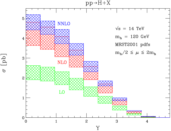
Figure 3: Bin-integrated Higgs boson rapidity distribution at the LHC. The bands indicate the scale choice $m_{h}/2\leq\mu\leq 2m_{h}$.

All the results that we present in this Section can be divided into two categories, depending on whether or not the decay of the Higgs boson into two photons is considered. We first study the simpler case, in which the Higgs boson is treated as a stable particle, and investigate the various kinematic distributions of the Higgs. We then turn to the analysis of the Higgs signal in the di-photon channel, and present the NNLO cross sections and the distributions in the pseudorapidity difference $|\eta^{\gamma,1}-\eta^{\gamma,2}|/2$ and the average transverse momentum $(p_{\bot}^{\gamma,1}+p_{\bot}^{\gamma,2})/2$ of the two photons.

The rapidity distribution of the Higgs boson with mass $m_{h}=120~{}{\rm GeV}$ is shown in Fig. 3 at LO, NLO, and NNLO in QCD perturbation theory. The bands are obtained by equating the factorization and the renormalization scales $\mu_{f}=\mu_{r}=\mu$, and then varying $\mu$ in the range $m_{h}/2\leq\mu\leq 2m_{h}$. We use the parton distribution functions (pdfs) from the MRST2001 set mrst , and employ mode 1 as the default mode for pdf evolution. Higher order QCD corrections to the Higgs rapidity distribution exhibit behavior similar to the corrections to the inclusive cross section; the large increase in ${\rm d}\sigma/{\rm dY}$ from LO to NLO, is not followed by a similar large increase from NLO to NNLO. The NNLO corrections are uniform over the central rapidity interval $|Y|<2$, and can therefore be obtained to good approximation by re-scaling the NLO rapidity distribution by a universal, rapidity-independent factor.

For a Higgs boson heavier than $\sim 140~{}{\rm GeV}$, the decay $H\to W^{+}W^{-}$ becomes the dominant decay mechanism, making the Higgs branching ratio into two photons quite small; consequently, the two photon signal can not be used as the primary trigger for the Higgs. Searching for the Higgs boson in the $W^{+}W^{-}$ decay mode requires the introduction of additional cuts to suppress the background due to the production and subsequent decay of a pair of top quarks. Since the hadronic jets in top pair production have, on average, larger transverse momenta than hadronic jets in Higgs hadroproduction, the significance of the Higgs signal can be enhanced by imposing a jet veto on the recoiling hadronic system veto ; vetoexp . In Fig. 4 we present the rapidity distribution of the Higgs boson with mass $m_{h}=150~{}{\rm GeV}$, when all jets in the final state of the reaction $pp\to H+X$ are required to have transverse momenta smaller than $p^{\rm jet}_{\rm T,veto}=40~{}{\rm GeV}$. The jets are identified with the cone algorithm, using a cone size $R=0.4$.

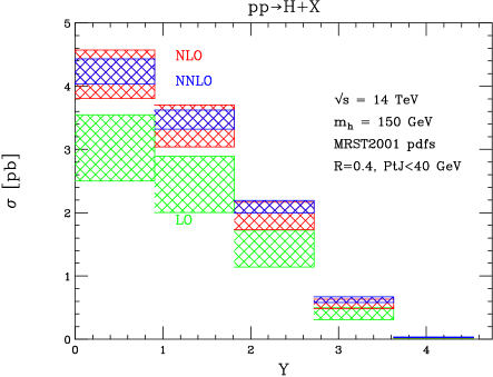
Figure 4: Bin-integrated Higgs boson rapidity distributions at the LHC with a jet veto applied.

It is instructive to compare both the magnitude of the perturbative corrections and the residual scale dependence of the Higgs rapidity distributions with and without the jet veto. Although Figs. 3,4 refer to different masses of the Higgs boson, a qualitative comparison is still possible; as is known from the NNLO computation of the inclusive cross section, the relative magnitude of the NNLO corrections does not depend strongly on the Higgs boson mass. From Figs. 3,4 we observe that the application of the jet veto leads to a better perturbative stability of the rapidity distribution; the perturbative corrections are smaller when the jet veto is applied, and there is a complete overlap of the NNLO scale dependence band with the NLO band, for most rapidities. This comparison shows that large and perturbatively unstable contributions to the Higgs boson hadroproduction cross section are related to kinematic configurations where the Higgs is produced with large transverse momentum. This feature does not imply a breakdown of the perturbative expansion; it merely reflects the fact that for Higgs hadroproduction, the leading order partonic process is $gg\to H$, so that at LO the Higgs boson is produced with zero transverse momentum. Therefore, if Higgs boson production with $p_{\bot}^{\rm higgs}\neq 0$ is considered, our NNLO computation includes just two terms in the perturbative expansion in the strong coupling constant, and is therefore a NLO computation.

The excellent convergence observed for the jet-vetoed rapidity distribution with $p^{\rm jet}_{\rm T,veto}=40~{}{\rm GeV}$ is partly accidental. This can be seen from Fig. 5, where we show the dependence of the Higgs boson production cross section on the value of a veto on the transverse energy of the Higgs, $p_{\rm T,veto}$. While the LO cross section obviously does not depend on $p_{\rm T,veto}$, both the NLO and the NNLO cross sections exhibit a significant dependence on this parameter. It is interesting to observe that the NLO cross section reaches its asymptotic value much faster than the NNLO one; this is related to the fact that the average $p_{\rm T}$ of the Higgs boson increases from NLO to NNLO. For example, for $m_{h}=150~{}{\rm GeV}$, the average transverse momenta of the Higgs boson at NLO and NNLO are $\langle p_{\bot}^{\rm NLO}\rangle=37.5~{}{\rm GeV}$ and $\langle p_{\bot}^{\rm NNLO}\rangle=44.6~{}{\rm GeV}$. It is clear from Fig. 5 that the choice $p_{\rm T,veto}=40~{}{\rm GeV}$ minimizes the NNLO QCD corrections for $m_{h}=150~{}{\rm GeV}$. However, other choices of $p_{\rm T,veto}$ also lead to only small differences between the NLO and the NNLO cross sections, indicating an improved convergence of the perturbative expansion for all veto choices.

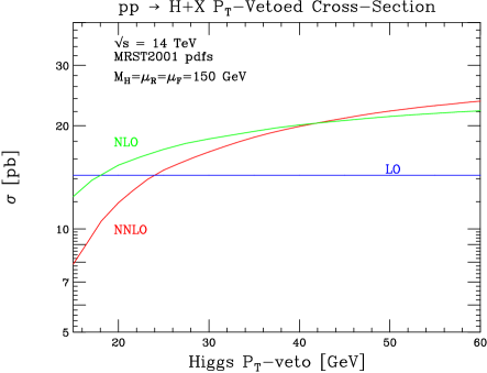
Figure 5: The Higgs boson production cross section at the LHC as a function of $p_{\rm T,veto}$.

Another interesting feature of the NNLO result is the dependence of the jet-vetoed cross section on the cone size $R$. At NLO, every jet is associated with a massless gluon or quark, so there is no cone-size dependence of the cross section. At NNLO, when two partons are close in rapidity and azimuthal angle, they are combined into a single jet. Thus, a cone-dependence of the observable cross section appears. As can be seen from Fig. 6, the cross section decreases when the cone size is increased over a large range of $R$; however, at large values of $R$ the cross section starts to increase again. This is a consequence of the fact that, originally, combining two energetic partons into a single jet increases its transverse momentum. However, after the cone size becomes so large that two partons which are back-to-back in the transverse plane are combined to form a single jet, the momentum of such a jet becomes smaller than the momenta of the individual partons. This effect drives an increase in the cross section for $R\geq 2.5$.

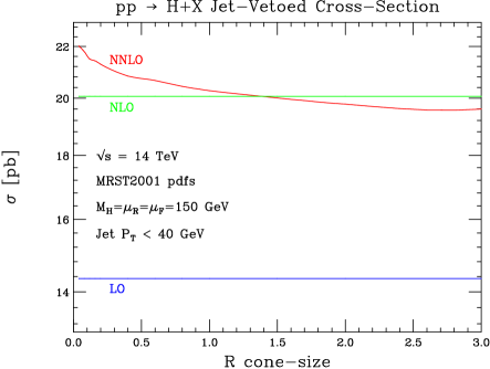
Figure 6: The Higgs boson production cross section at the LHC with a jet-veto of $p_{\rm T,veto}=40~{}{\rm GeV}$, as a function of the cone size $R$.

Since the rapidity of the Higgs boson is not probed, the results of Fig. 6 can also be obtained veto by subtracting the NLO contributions for $H+1\mbox{ jet}$ production deFlorian:1999zd ; Campbell:2000bg from the NNLO total cross section. We have compared our results with those in Refs. deFlorian:1999zd ; Campbell:2000bg , and have found excellent agreement.

We now discuss the Higgs boson signal in $pp\to H+X\to\gamma\gamma+X$. An interesting observable is the total di-photon production cross section, subject to a number of cuts on the kinematic variables of the two photons. These cuts, designed to enhance the signal over the prompt photon background, include restrictions on the photon transverse momenta and the rapidities, as well as isolation cuts. In particular, the photons are required to have transverse momenta $p_{\bot}^{(1)}\geq 40~{}{\rm GeV}$ and $p_{\bot}^{(2)}\geq 25~{}{\rm GeV}$; they must also be produced in the central rapidity region $|\eta|<2.5$ search . The isolation cuts are designed to reduce contamination of the signal by the poorly known fragmentation contributions. We require that a photon candidate does not have an additional transverse energy $E_{\rm T}$ which is greater than $E_{\rm T,min}=15~{}{\rm GeV}$ deposited within a cone around it of radius $R_{\rm is}=\sqrt{(\eta-\eta_{\gamma})^{2}+(\phi-\phi_{\gamma})^{2}}=0.4$. We will refer to this combination of cuts as the “standard photon cuts” in what follows.

$$\begin{array}[]{||c|c|c||c|c||c|c||}\hline\cr&\vrule\lx@intercol\hfil\sigma_{\rm LO}/Br_{\gamma\gamma},~{}{\rm pb}\hfil\lx@intercol\vrule\lx@intercol&\vrule\lx@intercol\hfil\sigma_{\rm NLO}/Br_{\gamma\gamma},~{}{\rm pb}\hfil\lx@intercol\vrule\lx@intercol&\vrule\lx@intercol\hfil\sigma_{\rm NNLO}/Br_{\gamma\gamma},~{}{\rm pb}\hfil\lx@intercol\vrule\lx@intercol\\ \cline{2-7}\cr m_{h},~{}{\rm GeV}&\mu=m_{h}/2&\mu=2m_{h}&\mu=m_{h}/2&\mu=2m_{h}&\mu=m_{h}/2&\mu=2m_{h}\\ \hline\cr\hline\cr 110&16.10&11.67&31.33&23.12&33.53&27.68\\ \cline{2-7}\cr 115&15.59&11.23&29.75&21.97&31.40&26.80\\ \cline{2-7}\cr 120&15.02&10.76&28.30&20.93&29.51&25.67\\ \cline{2-7}\cr 125&14.40&10.27&26.94&19.92&28.58&24.56\\ \cline{2-7}\cr 130&13.79&9.79&25.52&19.03&27.92&23.29\\ \cline{2-7}\cr 135&13.19&9.32&24.31&17.99&26.04&22.05\\ \cline{2-7}\cr\hline\cr\end{array}$$

Table 1: The cross section for $pp\to H+X\to\gamma\gamma+X$, divided by the branching ratio $Br(H\to\gamma\gamma)$, at $\sqrt{s}=14~{}{\rm TeV}$ with the standard cuts applied to the photons, for different values of the Higgs mass.

$$\begin{array}[]{||c|c|c||}\hline\cr m_{h},~{}{\rm GeV}&\sigma^{\rm cut}_{\rm NNLO}/\sigma^{\rm inc}_{\rm NNLO}&K^{(2)}_{\rm cut}/K^{(2)}_{\rm inc}\\ \cline{1-3}\cr 110&0.590&0.981\\ \cline{2-3}\cr 115&0.597&0.968\\ \cline{2-3}\cr 120&0.603&0.953\\ \cline{2-3}\cr 125&0.627&0.970\\ \cline{2-3}\cr 130&0.656&1.00\\ \cline{2-3}\cr 135&0.652&0.98\\ \cline{2-3}\cr\hline\cr\end{array}$$

Table 2: Comparisons between the cut and inclusive cross sections for different Higgs masses. The second column contains the ratio of the NNLO cross section with the standard cuts over the inclusive cross section, while the third column contains the ratio of cut and inclusive results for the $K$-factor $K^{(2)}=\sigma_{\rm NNLO}/\sigma_{\rm NLO}$. We have set $\mu=m_{h}/2$.

In Table 1 we present the cross section for $pp\to H+X\to\gamma\gamma+X$, divided by the branching fraction of $H\to\gamma\gamma$, with the standard cuts imposed on the photons. We give results through LO, NLO and NNLO in perturbation theory, for different Higgs boson masses and for two choices of the renormalization and factorization scales. The NNLO results are accurate to 1%, while the LO and NLO numbers are accurate to 0.1%. The perturbative corrections to the di-photon signal follow the pattern of the corrections to the inclusive Higgs production cross section. We note the apparent convergence of the di-photon signal, with the NNLO corrections increasing the NLO result by up to $\sim 20\%$, depending on the value of $\mu$ and the Higgs boson mass. The NNLO and NLO scale dependence bands overlap significantly, and the NNLO scale dependence is reduced by a factor of two compared to the NLO dependence.

It is interesting that the NNLO corrections are much smaller when the scale $\mu=m_{h}/2$ is chosen. This is in accord with the observation that the typical transverse momentum of the Higgs boson is parametrically smaller than the Higgs mass $m_{h}$; because of the rapid increase of the gluon pdf at low $x$, the Higgs bosons are produced close to threshold. Since the factorization scale should be chosen close to a typical transverse momentum of the Higgs, selecting $\mu=m_{h}/2$ expedites the convergence of the perturbative expansion. Fig. 7 shows the dependence of the Higgs signal on the choice of the scale for $m_{h}=120~{}{\rm GeV}$. As expected, we find that the NNLO perturbative corrections are small for $\mu\sim 40-50~{}{\rm GeV}$. We note that the threshold resummed results for the Higgs hadroproduction cross section Catani:2003zt agree very well with the fixed order results for smaller scale choices such as $\mu\sim m_{h}/2$, while they differ from the fixed order results by up to several percent for larger scale choices. It appears, from the stability of the perturbative series and the agreement with the resummed result, that $\mu\sim m_{h}/2$ is a better scale choice for Higgs hadroproduction.

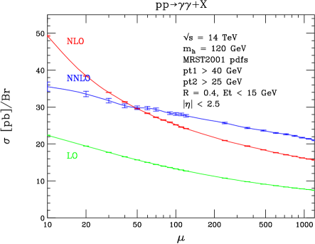
Figure 7: The Higgs channel $pp\to H+X\to\gamma\gamma+X$ with the standard cuts imposed on the photons, as a function of scale choice.

In Table 2 we present several comparisons between the inclusive NNLO cross section, and the NNLO cross section computed with the standard cuts. Our goal in doing this is two-fold: to understand how the cross section is affected by the standard cuts, and to see how well the realistic cut cross section can be approximated if only the inclusive NNLO result is known. We adopt $\mu=m_{h}/2$ for these comparisons. These results are valid to approximately 2%. In the second column of Table 2 we have presented the ratio of the NNLO cross section with the standard cuts over the inclusive NNLO result. The reduction of the cross section caused by the cuts ranges from 40% for $m_{h}<120$ GeV to 30% for $m_{h}>150$ GeV. We note that most of this reduction comes from the $p_{\bot}$ and $\eta$ cuts; the isolation cuts decrease the ratio by less than 3%. This is expected; there is no cross section enhancement when a parton is emitted along the photon direction, so this phase-space region contributes minimally to the total result. We note that the cuts become less effective at larger $m_{h}$, i.e., the ratio increases. For larger Higgs masses, the average photon $p_{\bot}$ increases, and therefore more events pass the cuts.

In the third column of Table 2 we present the ratio of the $K$-factor $K^{(2)}=\sigma_{\rm NNLO}/\sigma_{\rm NLO}$. This is interesting for the following reason. Suppose only the differential NLO cross section and the inclusive NNLO result are known. The best approximation for the exact NNLO differential result would then be $d\sigma^{\rm approx}_{\rm NNLO}=d\sigma_{\rm NLO}\times K^{(2)}_{\rm inc}$, where $K^{(2)}_{\rm inc}$ is defined with the inclusive cross sections. Calculating the cut cross section with this distribution gives $\sigma^{\rm approx,cut}_{\rm NNLO}=\sigma^{\rm cut}_{\rm NLO}\times K^{(2)}_{\rm inc}$. The ratio of this result with the exact NNLO cross section with the standard cuts imposed is $\sigma^{\rm cut}_{\rm NNLO}/\sigma^{\rm approx,cut}_{\rm NNLO}=K^{(2)}_{\rm cut}/K^{(2)}_{\rm inc}$; the deviation of this ratio from unity measures the error made by using $d\sigma^{\rm approx}_{\rm NNLO}$ to approximate the actual differential cross section at NNLO. We see that this deviation is less than about 5%.

In order to optimize the experimental cuts, it is desirable to have a good understanding of the kinematic distributions of the photons, since they can provide good discriminators between the signal and the background. While we do not discuss cut optimization in this paper, we present two differential distributions that illustrate the range of observables that can be studied using our calculation. In Fig. 8, the $p_{\bot}=(p_{\bot}^{\gamma,1}+p_{\bot}^{\gamma,2})/2$ distribution is shown for $m_{h}=120~{}{\rm GeV}$. We observe large perturbative corrections close to the kinematic boundary at leading order, $p_{\bot}<m_{h}/2=60~{}{\rm GeV}$, where resummation of large logarithms is required. However, the presence of a large peak near the LO kinematic boundary appears to be a reliable result, as it appears without drastic modification at both NLO and NNLO. Since the background should not contain any such feature, this is potentially a useful discriminating variable.

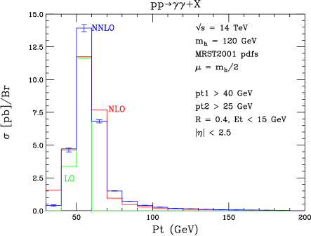
Figure 8: The $p_{\bot}=(p_{\bot}^{\gamma,1}+p_{\bot}^{\gamma,2})/2$ distribution for the di-photon Higgs signal at the LHC.

In Fig. 9, we present the distribution of the pseudorapidity difference $Y_{s}=|\eta^{\gamma,1}-\eta^{\gamma,2}|/2$ between the two photons. This distribution is interesting since a similar distribution from the prompt photon production background is flatter; this information can be used to enhance the statistical significance of the Higgs signal lance1 . From Fig. 9 we see that the peak at $|\eta^{\gamma,1}-\eta^{\gamma,2}|=0$ is also present when the NNLO effects are included.

Figure 9: The distribution in the pesudorapidity difference of the two photons, $Y_{s}=|\eta_{1}^{\gamma}-\eta_{2}^{\gamma}|/2$.

The results presented in this Section are for the di-photon Higgs signal. There are other Higgs decay modes that are of significant interest. In particular, for moderately heavy Higgs bosons, decays into $ZZ\to 4l$ and $W^{+}W^{-}\to l^{+}l^{-}\nu_{l}\bar{\nu}_{l}$ might provide suitable channels for discovery. Since our calculation retains all the information about the Higgs boson kinematics, it is in principle straightforward to include Higgs decays into arbitrary final states. However, in reality, some care must be exercised to generate the final-state decay efficiently, especially for decays with high multiplicities and sophisticated cuts. We plan on adding additional Higgs decay channels to our code in the future.

X Description of the FORTRAN code

In this Section we describe a FORTRAN program, FEHiP, which we have written to obtain the results described in the previous Section. As can be seen from the examples presented there,  FEHiP computes the cross section for Higgs boson production in hadronic collisions through NNLO in perturbative QCD in the presence of an arbitrary measurement function. The decays of the Higgs are treated in the narrow width approximation. At present, only the Higgs decay into two photons is included; other decays can be added. This Section provides instructions for using the code.

X.1 Download and Compile

The code can be downloaded from codeloc . To compile the code, first uncompress the file fehip.tar.gz and run the “make” script:

        \home\user> tar -zxvf fehip.tar.gz
        \home\user> cd FEHIP
        \home\user\FEHIP> make

We have sussesfully compiled the code on Linux systems using the GNU g77 compiler. To compile the code on other platforms the user should modify the file makefile. To run the code, execute the program fehip:

        \home\user\FEHIP> fehip

The program performs multidimensional numerical integrations using the adaptive Monte Carlo algorithm Vegas vegas ; we use its recent implementation in the CUBA library cuba . The current version of this library, Cuba-1.0, is included in the distribution of  FEHiP, and compiles automatically with the above make script. For future updates of the Cuba library, we refer the user to cuba ; the directory FEHiP$\backslash$Cuba-1.0$\backslash$ and the file makefile should be updated appropriately.

X.2 Basic parameters and Usage

The basic parameters that are used by  FEHiP include the mass of the Higgs boson, the type and energy of the hadron collider, the factorization and renormalization scales, and the order in perturbation theory through which the result is to be computed. The code also requires the mass of the top quark and the value of the Fermi constant to compute the normalization of the Higgs boson production cross section (cf. Eq.(85)). This input is provided by the user in the file input.txt.

A prototype input file has the following format:

’Mass of the Higgs boson (GeV) = ’ 120d0
=============================================
’Collider (pp=0, ppbar=1)      = ’ 0
’CMS collision energy (GeV)    = ’ 14000d0
=============================================
’Factorization scale  (GeV)    = ’ 120d0
’Renormalization scale  (GeV)  = ’ 120d0
=============================================
’Top-quark mass (GeV)          = ’ 175d0
’Fermi constant  =             = ’ 0.0000116639d0
=============================================
’Final-state (0=no-decay, 1=diphoton) = ’ 1
’Branching ratio                      = ’ 1d0
=============================================
’Perturb. Order (0=LO, 1=NLO, 2=NNLO) = ’ 1
=============================================
’Output File                   =’  ’result.dat’

The user should provide values for the following variables:

• The mass of the Higgs boson. This is a double precision variable that sets the value of the Higgs boson mass $m_{h}$, in GeV.

• Collider. An integer variable that defines the type of collider. For proton-proton collisions, the value must be set to 0; for proton-antiproton collisions, the value must be set to 1.

• Energy. A double precision variable for the energy of the collider, in GeV.

• Factorization scale. A double precision variable for the value of the factorization scale $\mu_{F}$, in GeV.

• Renormalization scale. A double precision variable for the value of the renormalization scale $\mu_{R}$, in GeV.

• Top-quark mass. A double precision variable for the value of the top-quark mass $m_{t}$, in GeV.

• Fermi-constant. A double precision variable for the value of the Fermi constant $G_{F}$, in $\mbox{\rm GeV}^{-2}$.

• Final-state. An integer variable that determines the decay mode of the Higgs boson. The value 0 corresponds to the “no-decay” option. In this case it is assumed that the Higgs boson four momentum is fully reconstructed and is therefore an observable. With the “no-decay” option, it is possible to impose cuts on the transverse momentum and the rapidity of the Higgs boson, and to study jet-clustering and jet-veto cuts for the additional radiation (of up to $2$ partons) in the final-state. However, no information about the kinematics of the Higgs decay product is provided.

  The value 1 corresponds to the “diphoton decay mode”. In this case, the Higgs decays into two photons in the narrow width approximation, and the kinematics of the two photons in the final state is fully reconstructed. Hence, arbitrary cuts on the photon momenta can be imposed.

  We note that the results for the “no-decay” mode can always be obtained from the “decay” mode. Indeed, if no restrictions on the momenta of the individual photons are imposed, the two options should provide identical results. However, if one is not interested in the kinematics of the Higgs decay product, it is beneficial to declare the “no-decay” option explicitly, since the dimensionality of the numerical integration performed is then lowered.

  Finally, we note that in the future, additional decays of the Higgs boson will be added to the program.

• Branching ratio. A double precision variable for the value of the branching fraction of the Higgs boson decay into the selected final state. The program computes the Higgs production cross section in the narrow-width approximation and multiplies the output by the ‘Branching ratio’. The value of the branching fraction for a particular decay of the Higgs with a certain mass should be supplied by the user as an input. Theoretical predictions for the branching fractions of the Higgs can be obtained with the program HDECAY hdecay .

• Perturbative Order. An integer variable which sets the order through which the perturbative expansion of the Higgs boson production cross section is computed. The values 0, 1, and 2 correspond to the LO, NLO, and NNLO cross sections, respectively.

• Output File. A character string variable for the file name where the results of the calculation are written. The output file has the following format:

   proton-proton collider
   CMS collision Energy =   14000.
   ==================================
   Higgs boson mass =   120.
   Factorization scale =   120.
   Renormalization scale =   120.
   ==================================
   Top-quark mass =   175.
   Fermi constant =   1.16639E-05
   ==================================
   H --> gamma gamma
   Branching Ratio =   1.
   ==================================
   NLO Cross Section
   Strong coupling =   0.114230586
   ==================================
  
   ===========   RESULT    =================
   sigma =  38.4079658  +/-    0.0362102225
   chi square probability =  2.46758092E-05
   =========================================
  

  It contains a description of the input parameters and the result (sigma) for the cross section in picobarns with the corresponding statistical error from the Vegas integration. It also provides the $\chi^{2}-$probability (prob variable from the Vegas routine in CUBA), which is an indicator of the reliability of the Monte-Carlo integration.

A number of other necessary program settings and options are not included in the user controlled input.txt file. Some important settings can be found in the main program file higgs.F; we have set them to values that are reasonable for practical purposes, according to our own experience with the code. In this file, we define the parameters for Vegas, compute the normalization of the cross section, and invoke the integration routine. For example, we require a precision (the epsrel variable) of $1\%$ at NNLO and of $0.1\%$ at lower orders with an absolute error above $[10^{-3}\times Br]\;pb$. We note that  FEHiP  also writes the iteration-by-iteration results produced by Vegas to screen, so the user can track the output; this can easily be redirected to a separate file. This can be suppressed by modifying the appropriate flag in higgs.F; we refer the reader to the CUBA documentation for a discussion of the various output options.

FEHiP uses the MRST 2001 LO, NLO, and NNLO parton distribution functions mrst . These are provided with the distribution of  FEHiP. We note that it is extremely inefficient to directly call the pdf routines. Since the factorization scale and the range of the Bjorken variable $x$ are fixed during each run of the program, we only need a limited amount of information about the pdfs. To optimize the code, we adopt the following strategy. When the code is initialized,  FEHiP first calls the pdf routines for a given value of the factorization scale and computes the pdfs for $1000$ different choices of $x$. The distribution of these points is not uniform; we increase their density for $x$ values where the pdfs change rapidly. We then use interpolation with quadratic polynomials to connect the adjacent points. Consequently, each pdf is described by an array of coefficients of these quadratic polynomials which is kept in memory; this speeds up the execution of  FEHiP enormously. We have tested that the approximate pdf values are accurate to better than $0.05\%$ for all $x$ and $\mu_{F}$ values relevant for Higgs production.

To use a different set of pdfs, the user should replace the mrstpdfs.F file with the appropriate set, and modify the calls to the mrstlo, mrst2001, and mrstnnlo subroutines in the file fitpdf.F. In addition, the user should change the value of $\alpha_{s}\left(M_{Z}\right)$, which is used as an initial condition for the LO ,NLO, and NNLO evolution of the strong coupling, to the value which is consistent with the fitting of the new pdf set. The variables asZlo, asZnlo, and asZnnlo in the file higgs.F correspond to the fitted values for the MRST 2001 LO, NLO, and NNLO pdfs.

X.3 Experimental cuts

The most complicated user input is the definition of the experimental observable; this requires imposing cuts on the phase-space of the final state. We describe here a double precision function, named constraint, in the constraint.F file, which can be used for this purpose.

The constraint function corresponds to the observable function $F_{J}$ for the final state. The NNLO parton multiplicity is assumed:

$$\mbox{parton}_{1}(p_{1})+\mbox{parton}_{2}(p_{2})\to H(p_{h})+\mbox{parton}_{3}(p_{3})+\mbox{parton}_{4}(p_{4}).$$ (86)

All final-state configurations with lower multiplicities have been mapped to this “maximal” final state by introducing additional partons with zero momentum when needed; this allows a uniform introduction of cuts for both real and virtual corrections.

The routine uses the following (local and global) arguments :

• the Vegas-generated variables: var;

• the dimensionality ndim of the Vegas integration;

• the squared mass of the Higgs boson, m2 $=m_{h}^{2}$, and the CMS square energy of the colliding hadrons scm $=s$;

• the Bjorken variables x1, x2 and the ratio z $=\frac{m_{h}^{2}}{sx_{1}x_{2}}$;

• the variables s13,s23,s14,s24 with $s_{if}=-\frac{p_{i}\cdot p_{f}}{p_{1}\cdot p_{2}},\;i=1,2,\;f=3,4$, and the variable s34 $=\frac{p_{3}\cdot p_{4}}{p_{1}\cdot p_{2}}$;

• the variables s1v,s2v with $s_{iv}=\frac{(p_{i}-p_{h})^{2}}{2p_{1}\cdot p_{2}},\;i=1,2$;

• the variables s3v,s4v with $s_{vf}=\frac{(p_{f}+p_{h})^{2}}{2p_{1}\cdot p_{2}},\;f=3,4$.

From these variables we can reconstruct the components of the momenta of all particles in the final state, and impose cuts which define the observable. We can also generate (using the var array) the required additional phase-space variables for the subsequent decay of the Higgs boson.

After the appropriate variable declarations at the beginning of the routine, we proceed by generating phase-space variables for the two photons coming from the decay

$$H(p_{h})\to\gamma_{a}(q_{a})+\gamma_{b}(q_{b}),$$ (87)

using a convenient parameterization in terms of invariant masses formed from the photon momenta $q_{a,b}$ and the initial state partonic momenta $p_{1,2}$. The routine, for each Vegas event, computes the following quantities.

• The transverse energy of: (1) the Higgs boson, pT; (2) parton 3, pt3; (3) parton 4, pt4; (4) $\gamma_{a}$, ptga; (5) $\gamma_{b}$, ptgb.

• The energy of: (1) the Higgs boson, En; (2) parton 3, En3; (3) parton 4, En4; (4) $\gamma_{a}$, Ena; (5) $\gamma_{b}$, Enb.

• The momentum along the beam axis of: (1) the Higgs boson, pZ; (2) parton 3, pz3; (3) parton 4, pz4; (4) $\gamma_{a}$, pza; (5) $\gamma_{b}$, pzb.

The above variables can be defined for all events, including the ones where unresolved (soft/collinear) partons and photons are generated in the final state. However, the pseudorapidity and relative angles of massless particles can be sensibly defined only if they are resolved. To discriminate, we introduce a cutoff for the transverse energy of photons and partons in the final state, ptbuf $=0.01{\rm GeV}$. We then use two flags, topflag and photonflag, to characterize the event according to how many partons and photons have a transverse energy above the cutoff. For every event we define:

• topflag = 0d0: two unresolved partons in the final state, pt3,pt4 < ptbuf.

• topflag = 1d0: one resolved and one unresolved parton in the final state, pt3 < ptbuf, pt4 > ptbuf or pt4 < ptbuf, pt3 > ptbuf. For such an event we compute the additional variables:

  • the transverse energy of the resolved parton: ptr.

  • the rapidity of the resolved parton: etar.

• topflag = 2d0: two resolved partons pt3,pt4 > ptbuf, and the Higgs boson with non-zero transverse energy, pT > 0. For this event we also compute:

  • the pseudo-rapidity of parton 3, eta3, and parton 4, eta4.

  • the azimuthal angle between parton 3 and parton 4: phi34.

• topflag = 3d0: corresponds to the (rare) configuration with two resolved partons, pt3,pt4 > ptbuf, and the Higgs boson with zero transverse energy, pT = 0. For this event we also compute:

  • the pseudo-rapidity of parton 3, eta3, and parton 4, eta4.

We also define:

• photonflag = 0d0: at least one unresolved photon in the final state, ptga < ptbuf or ptgb < ptbuf.

• photonflag = 1d0: corresponds to two resolved photons ptga,ptgb > ptbuf, and the Higgs boson with non-zero transverse energy pT > 0. For this event we also compute:

  • the pseudo-rapidity of $\gamma_{a}$, etaa, and $\gamma_{b}$, etab.

• photonflag = 2d0: two resolved photons pt3,pt4 > ptbuf, and the Higgs boson with zero transverse energy, pT = 0. For this event we also compute:

  • the pseudo-rapidity of $\gamma_{a}$, etaa, and $\gamma_{b}$, etab.

In order to study the isolation of photons, the routine computes the relative azimuthal angles of resolved photons with resolved partons. This can be done for the following combinations of flag values.

• photonflag = 1d0,2d0 and topflag = 2d0: The program computes the azimuthal angles for the pairs

  • $\gamma_{a},\mbox{parton}_{3}$: angle phi3a.

  • $\gamma_{b},\mbox{parton}_{3}$: angle phi3b.

  • $\gamma_{a},\mbox{parton}_{4}$: angle phi4a.

  • $\gamma_{b},\mbox{parton}_{4}$: angle phi4b.

• photonflag = 1d0 and topflag = 1d0: The program computes the azimuthal angles for the pairs

  • $\gamma_{a},\mbox{resolved parton}$: angle phira.

  • $\gamma_{b},\mbox{resolved parton}$: angle phirb.

The above variables completely describe the phase-space for Higgs production and decay into photons through NNLO, and can be used to implement standard experimental cuts. We now describe the structure of constraint.F, and indicate how the reader modify the file to include other cuts.

The section of constraint.F marked as STEP 1 performs the generation of the photon phase-space. STEP 2 computes the variables we have just described. We have placed the cuts required for the numerical results of this paper in the section labeled STEP 3: IMPLEMENTATION OF CUTS. These are:

• the Higgs boson rapidity cut;

• the Higgs boson $p_{T}$ cut;

• the jet-veto;

• cuts on the pseudorapiditiy and $p_{T}$ of each photon;

• an isolation veto on each photon;

• a cut on the average $p_{T}$ of the photons;

• a cut on the pseudorapidity difference of the photons.

An event is accepted if the constraint function returns the value 1d0, and rejected when it returns 0d0. Before any cut is applied, the value of the function is set to 1d0. Cuts are applied successively; each cut could potentially reject the event by setting the function value to 0d0. To control which cuts should be applied to the event, we use two flags: active, inactive. The user can choose combinations of the above cuts by modifying the appropriate flags, as described in constraint.F.

The cuts that are programmed in STEP 3 of the routine serve as guiding examples for the user. When programming a new cut, some care is required for constraints on variables which are only defined when a final state particle is resolved; the user should provide that the constraint function returns an appropriate value for the events where the probed variable is not defined. In the section labeled STEP 4 of the constraint.F file, we have placed a “general” cut to guide the reader through this process. By modifying this section, it is possible to impose any desired constraint on the final state.

X.4 Other information

To summarize, the user input for  FEHiP is a set of parameters in the input.txt file, and the constraint function in the constraint.F file. To run the program, the user should compile using the make script and execute fehip. The make script should be executed every time that the constraint.F file is modified.

We now describe some standard running times for the observables considered in this paper. We measure run times using the number of Vegas evaluations required to reach a given precision; on a 3 GHz PC, $10^{5}$ evaluations takes approximately 1 hour. The required number of evaluations for observables in the “no-decay” mode is typically fairly small. To reach 1% precision on the fully inclusive NNLO cross section at the LHC, about $1.5-2\times 10^{5}$ evaluations are needed. To reach 1% precision on a jet-vetoed cross section, about $8\times 10^{5}$ evaluations are needed. These numbers increase dramatically when the “decay” mode is used, and the standard cuts on the photons are imposed. For 1% precision on the $pp\rightarrow H+X\rightarrow\gamma\gamma+X$ cross section with $p_{T}$, $\eta$, and isolation cuts imposed, $7\times 10^{6}$ evaluations are required. Computing bins for photon distributions to 2% or better precision usually takes over $10^{7}$ evaluations.

Clearly, some observables require long running times. If the program is interrupted, the user can restart it by executing fehip. The CUBA library saves in a file the data of every Vegas iteration; this is used to restart the program from the last completed iteration. To force the program to restart from the first Vegas iteration, the user should type make clean and then execute fehip.

XI Conclusions

We have discussed the calculation of the Higgs boson production cross section in hadronic collisions through NNLO in perturbative QCD. The kinematics of both the Higgs and the QCD radiation is kept exactly. This allows us to consider any decay of the Higgs, and impose arbitrary cuts on the final state. In this paper, we have focused on Higgs decays into two photons. We stress that this calculation provides the first example of a fully realistic NNLO calculation of the Higgs signal in the di-photon channel, where the two photons in the final state satisfy all the selection criteria (cuts on photon pseudorapidities, transverse momenta, and geometric isolation from significant hadronic activity) used by the ATLAS and CMS collaborations.

To perform this calculation, we used the method of handling double real radiation described by us in sector ; Anastasiou:2004qd . We have further developed the approach in this paper, and have described its application to Higgs hadroproduction in detail.

We have given a description of the FORTRAN code  FEHiP which we used to obtain all the numerical results presented in this paper. The code can be obtained from codeloc . We hope that  FEHiP will be used when state-of-the-art knowledge of the Higgs signal at the LHC is required. In particular, since arbitrary cuts on the two photons and accompaning hadronic radiation are allowed, the code can be used to optimize cuts to enhance the signal-to-background ratio.

It was possible to obtain the results reported in this paper by further developing the approach suggested in sector ; Anastasiou:2004qd . Since this computation is far more complex than those considered in sector ; Anastasiou:2004qd , we believe that this is an important milestone for our approach. However, further development of the method is desirable. We give below a discussion from this perspective. We indicate areas where more work is required, and describe possible solutions to the problems of the method. We begin by listing attractive features of this approach.

• Given a convenient parameterization of the phase-space for the real emission contribution to a given process, the singularities are extracted in an automated fashion; the human intervention required to achieve the final result is minimal. No classification of the various singular regions is required. Similarly, the cancellation of singularities is performed completely numerically, without the need for any analytic integrations. In principle, this method therefore provides an algorithm for the extraction and cancellation of singularities through the ${\rm N^{n}LO}$ order in perturbation theory.

• Not only “real” singularities, but also some integrable ones are written in a factorized form. Consider the integral

  $$I_{1}=\int\limits_{0}^{1}\frac{{\rm d}x{\rm d}y~{}x^{\epsilon}}{x+y}.~{}~{}~{}$$ (88)

  Although the singularity at the point $x\sim y\sim 0$ in $I_{1}$ is integrable, we can apply the algorithm described in Section VII to it anyway. $I_{1}$ then becomes

  $$I_{1}=I_{1}^{(a)}+I_{1}^{(b)},~{}~{}~{}~{}I_{1}^{a}=\int\limits_{0}^{1}\frac{{\rm d}x{\rm d}y~{}x^{\epsilon}}{1+y},~{}~{}~{}I_{1}^{b}=\int\limits_{0}^{1}\frac{{\rm d}x{\rm d}y~{}(xy)^{\epsilon}}{1+x}.$$ (89)

  It is clear that the integrals $I_{1}^{(a,b)}$ are now written in forms very convenient for numerical evaluation. In addition to extracting real singularities, our technqiue also smooths integrable singularities, thereby improving the numerical behavior of the integrand.

• The complete kinematic information of the process is preserved. In principle, this enables us to use this result to construct a partonic level Monte-Carlo event generator.

In spite of these attractive features, there are also some problems with this approach.

• The most important drawback of the method is that it produces large expressions, which require long run-times for numerical evaluation and lead to difficulties with optimizing the code. Unfortunately, this is a natural feature of the approach; as we pointed out earlier, each time an entangled or line singularity is extracted, the expression size increases. However, it is useful to think of ways to ameliorate this behavior. It is instructive to recall how a somewhat similar problem was solved for NLO calculations. It was found that squaring matrix elements for unpolarized initial and final states is not a very practical option, since huge expressions are produced. Very compact expressions for scattering amplitudes can be obtained by working in the helicity basis. A similar approach can be attempted here. However, a given helicity amplitude contains terms that belong to different topologies, in the language of this paper. Since the separation into topologies is a crucial element of our approach, it is not clear how to to use helicity amplitudes efficiently.

• By default, this approach might give more information than desired. All possible contributions to the cross section are automatically obtained. For example, in the case of Higgs hadroproduction, we calculate $H+2~{}{\rm jets}$ at LO, $H+1~{}{\rm jet}$ at NLO and $H+0~{}{\rm jets}$ at NNLO. Imagine now that we want just the cross section of $H+1~{}{\rm jet}$ at NLO. Obviously, the number of entangled and line singularities we must deal with should be smaller. However, a blind application of the algorithm in Section VII will automatically handle all singularities, including those needed for $H+0~{}{\rm jets}$ at NNLO. It should be possible to implement additional criteria in the algorithm to prevent this from happening; for example, a check on the Higgs $p_{T}$ could be included, or a counting of the number of jets could be imposed. In the calculation of $e^{+}e^{-}\rightarrow 2$ jets at NNLO described in sector ; Anastasiou:2004qd , the $e^{+}e^{-}\rightarrow 3$ jets cross section at NLO can be obtained efficiently by including a call to the jet algorithm in the routine that handles singularities. However, a better understanding of these restrictions is needed before the approach can be used efficiently for processes with more complicated final states.

• Making a partonic level event generator out of our result is tedious, although possible. Because each sector corresponds to a different mapping of the invariant masses into $\lambda$-variables, each sector must be generated as a separate channel in a multi-channel Monte-Carlo. Our result for the Higgs hadroproduction cross section contains approximately a hundred sectors. In principle, this is not a problem, but it can definitely become an important issue in practice. The only solution to this issue that we can see is a better choice of phase-space parameterization, which leads to a smaller number of sectors.

Acknowledgments. We thank T. Hahn for helpful communications regarding the numerical integration package CUBA. We are grateful to Michael Peskin and Zoltan Kunszt for their help in finding the necessary computing resources, and the SLAC IT group for their technical support. We would like to thank John Campbell and Massimiliano Grazzini for comparisons. We are grateful to Guenther Dissertori and Zoltan Kunszt for useful suggestions and discussions. We would like to thank Michael Dittmar and Lance Dixon for pointing out mistakes in Figs. 7 and 9 in an earlier version of the paper. This work was started when the authors were visiting the Kavli Institute for Theoretical Physics, UC California, Santa Barbara. This research was supported by the US Department of Energy under contract DE-FG03-94ER-40833 and the Outstanding Junior Investigator Award DE-FG03-94ER-40833, and by the National Science Foundation under contracts P420D3620414350, P420D3620434350.

References

-
(1)
F. V. Tkachov, Phys. Lett. B100, 65 (1981);
K.G. Chetyrkin and F.V. Tkachov, Nucl. Phys. B192, 159 (1981). - (2) V. A. Smirnov, Phys. Lett. B 460, 397 (1999); J. B. Tausk, Phys. Lett. B 469, 225 (1999); V. A. Smirnov and O. L. Veretin, Nucl. Phys. B 566, 469 (2000); C. Anastasiou, T. Gehrmann, C. Oleari, E. Remiddi and J.B. Tausk, Nucl. Phys. B580, 577 (2000); T. Gehrmann and E. Remiddi, Nucl. Phys. B580, 485 (2000); T. Gehrmann and E. Remiddi, Nucl. Phys. B601, 248 (2001); Nucl. Phys. B601, 287 (2001); T. Gehrmann and E. Remiddi, Nucl. Phys. B640, 379 (2002).
- (3) Z. Bern, L.J. Dixon and A. Ghinculov, Phys. Rev. D63, 053007 (2001); C. Anastasiou, E.W.N. Glover, C. Oleari and M.E. Tejeda-Yeomans, Nucl. Phys. B601, 318 (2001); Nucl. Phys. B601, 341 (2001); C. Anastasiou, E.W.N. Glover, C. Oleari and M.E. Tejeda-Yeomans, Nucl. Phys. B605, 486 (2001); E.W.N. Glover, C. Oleari and M.E. Tejeda-Yeomans, Nucl. Phys. B605, 467 (2001); Z. Bern, A. De Freitas and L.J. Dixon, JHEP 0109, 037 (2001); Z. Bern, A. De Freitas, L.J. Dixon, A. Ghinculov and H.L. Wong, JHEP 0111, 031 (2001); C. Anastasiou, E.W.N. Glover and M.E. Tejeda-Yeomans, Nucl. Phys. B629, 255 (2002); T. Binoth, E.W.N. Glover, P. Marquard and J.J. van der Bij, JHEP 0205, 060 (2002); Z. Bern, A. De Freitas and L.J. Dixon, JHEP 0306, 028 (2003); E.W.N. Glover and M.E. Tejeda-Yeomans, JHEP 0306, 033 (2003).
- (4) L.W. Garland, T. Gehrmann, E.W.N. Glover, A. Koukoutsakis and E. Remiddi, Nucl. Phys. B627, 107 (2002); L.W. Garland, T. Gehrmann, E.W.N. Glover, A. Koukoutsakis and E. Remiddi, Nucl. Phys. B642, 227 (2002).
- (5) S. Laporta, Int. J. Mod. Phys. A15, 5087 (2000).
- (6) F. Bloch and A. Nordsieck, Phys. Rev. 52, 54 (1937).
- (7) T. Kinoshita, J. Math. Phys. 3, 650 (1962).
- (8) T. D. Lee and M. Nauenberg, Phys. Rev. 133, B1549 (1964).
- (9) C. Anastasiou and K. Melnikov, Nucl. Phys. B 646, 220 (2002) [arXiv:hep-ph/0207004].
- (10) C. Anastasiou and K. Melnikov, Phys. Rev. D 67, 037501 (2003) [arXiv:hep-ph/0208115].
- (11) C. Anastasiou, L. J. Dixon and K. Melnikov, Nucl. Phys. Proc. Suppl. 116, 193 (2003) [arXiv:hep-ph/0211141].
- (12) C. Anastasiou, L. J. Dixon, K. Melnikov and F. Petriello, Phys. Rev. Lett. 91, 182002 (2003) [arXiv:hep-ph/0306192].
- (13) C. Anastasiou, L. Dixon, K. Melnikov and F. Petriello, Phys. Rev. D 69, 094008 (2004) [arXiv:hep-ph/0312266].
- (14) K. Melnikov and A. Mitov, Phys. Rev. D 70, 034027 (2004) [arXiv:hep-ph/0404143].
- (15) A. Mitov, arXiv:hep-ph/0410205.
- (16) G. Sterman and S. Weinberg, Phys. Rev. Lett. 39, 1436 (1977).
- (17) S. Catani and M. H. Seymour, Nucl. Phys. B 485, 291 (1997) [Erratum-ibid. B 510, 503 (1997)] [arXiv:hep-ph/9605323].
- (18) S. Catani, S. Dittmaier, M. H. Seymour and Z. Trocsanyi, Nucl. Phys. B 627, 189 (2002) [arXiv:hep-ph/0201036].
- (19) R. K. Ellis, D. A. Ross and A. E. Terrano, Nucl. Phys. B 178, 421 (1981); W. T. Giele and E. W. N. Glover, Phys. Rev. D 46, 1980 (1992); K. Fabricius, I. Schmitt, G. Schierholz and G. Kramer, Phys. Lett. B 97, 431 (1980); F. Gutbrod, G. Kramer and G. Schierholz, Z. Phys. C 21, 235 (1984); Z. Kunszt, A. Signer and Z. Trocsanyi, Phys. Lett. B 336, 529 (1994); Z. Kunszt and D. E. Soper, Phys. Rev. D 46, 192 (1992); K. Fabricius, I. Schmitt, G. Kramer and G. Schierholz, Z. Phys. C 11, 315 (1981); G. Kramer and B. Lampe, Fortsch. Phys. 37, 161 (1989); A. Bassetto, M. Ciafaloni and G. Marchesini, Phys. Rept. 100, 201 (1983); B. Bailey, J. F. Owens and J. Ohnemus, Phys. Rev. D 46, 2018 (1992); F. Aversa, P. Chiappetta, M. Greco and J. P. Guillet, Nucl. Phys. B 327, 105 (1989); F. Aversa, L. Gonzales, M. Greco, P. Chiappetta and J. P. Guillet, Z. Phys. C 49, 459 (1991); P. Chiappetta, R. Fergani and J. P. Guillet, Z. Phys. C 69, 443 (1996); W. T. Giele, S. Keller and E. Laenen, Phys. Lett. B 372, 141 (1996); S. D. Ellis, Z. Kunszt and D. E. Soper, Phys. Rev. D 40, 2188 (1989); S. D. Ellis, Z. Kunszt and D. E. Soper, Phys. Rev. Lett. 69, 1496 (1992); S. Frixione, Z. Kunszt and A. Signer, Nucl. Phys. B 467, 399 (1996).
- (20) D. A. Kosower, Phys. Rev. D 67, 116003 (2003) [arXiv:hep-ph/0212097].
- (21) D. A. Kosower, Phys. Rev. Lett. 91, 061602 (2003) [arXiv:hep-ph/0301069].
- (22) S. Weinzierl, JHEP 0303, 062 (2003) [arXiv:hep-ph/0302180].
- (23) S. Weinzierl, JHEP 0307, 052 (2003) [arXiv:hep-ph/0306248].
- (24) A. Gehrmann-De Ridder, T. Gehrmann and G. Heinrich, Nucl. Phys. B 682, 265 (2004) [arXiv:hep-ph/0311276].
- (25) A. Gehrmann-De Ridder, T. Gehrmann and E. W. N. Glover, Nucl. Phys. B 691, 195 (2004) [arXiv:hep-ph/0403057].
- (26) A. Gehrmann-De Ridder, T. Gehrmann and E. W. N. Glover, hep-ph/0407023.
- (27) W. B. Kilgore, Phys. Rev. D 70, 031501 (2004) [arXiv:hep-ph/0403128].
- (28) S. Frixione and M. Grazzini, arXiv:hep-ph/0411399.
- (29) S. Catani, Phys. Lett. B 427, 161 (1998) [arXiv:hep-ph/9802439].
- (30) G. Sterman and M. E. Tejeda-Yeomans, Phys. Lett. B 552, 48 (2003) [arXiv:hep-ph/0210130].
- (31) Z. Bern, L. J. Dixon, D. C. Dunbar and D. A. Kosower, Nucl. Phys. B 425, 217 (1994); D. A. Kosower, Nucl. Phys. B 552, 319 (1999); D. A. Kosower and P. Uwer, Nucl. Phys. B 563, 477 (1999); Z. Bern, V. Del Duca and C. R. Schmidt, Phys. Lett. B 445, 168 (1998); Z. Bern, V. Del Duca, W. B. Kilgore and C. R. Schmidt, Phys. Rev. D 60, 116001 (1999); S. Catani and M. Grazzini, Nucl. Phys. B 591, 435 (2000); D. A. Kosower, Phys. Rev. D 57, 5410 (1998); F. A. Berends and W. T. Giele, Nucl. Phys. B 313, 595 (1989); J. M. Campbell and E. W. N. Glover, Nucl. Phys. B 527, 264 (1998); S. Catani and M. Grazzini, Phys. Lett. B 446, 143 (1999); S. Catani and M. Grazzini, Nucl. Phys. B 570, 287 (2000); V. Del Duca, A. Frizzo and F. Maltoni, Nucl. Phys. B 568, 211 (2000).
- (32) C. Anastasiou, K. Melnikov and F. Petriello, Phys. Rev. D 69, 076010 (2004) [arXiv:hep-ph/0311311].
- (33) T. Binoth and G. Heinrich, Nucl. Phys. B 585, 741 (2000).
- (34) K. Hepp, Commun. Math. Phys. 2, 301 (1966).
- (35) M. Roth and A. Denner, Nucl. Phys. B 479, 495 (1996) [arXiv:hep-ph/9605420].
- (36) C. Anastasiou, K. Melnikov and F. Petriello, Phys. Rev. Lett. 93, 032002 (2004) [arXiv:hep-ph/0402280].
- (37) C. Anastasiou, K. Melnikov and F. Petriello, Phys. Rev. Lett., in press [arXiv:hep-ph/0409088].
- (38) M. Carena and H. E. Haber, Prog. Part. Nucl. Phys. 50, 63 (2003) [arXiv:hep-ph/0208209].
- (39) G. Altarelli and M. W. Grunewald, arXiv:hep-ph/0404165.
-
(40)
J.R. Ellis, M.K. Gaillard, D.V. Nanopoulos,
Nucl. Phys. B106, 292 (1976);
M.A. Shifman, A.I. Vainshtein, M.B. Voloshin and V.I. Zakharov, Sov. J. Nucl. Phys. 30, 711 (1979). - (41) J.F. Gunion, P. Kalyniak, M. Soldate and P. Galison, Phys. Rev. D34, 101 (1986); J.F. Gunion, G. L. Kane and J. Wudka, Nucl. Phys. B299, 231 (1988).
-
(42)
ATLAS collaboration, “Atlas detector and physics performance;
technical design report.”, vol. 2, report CERN/LHCC 99-15, ATLAS-TDR-15;
CMS collaboration. “CMS: The electromagnetic calorimeter, technical design report.”, report CERN/LHCC 97-33, CMS-TDR-4;
V. Tisserand, Ph.D. thesis, LAL 97-01. February 1997;
M. Wielers, “Isolation of photons.”, report ATL-PHYS-2002-004;
“Summary of the CMS potential for the Higgs boson discovery”, CMS NOTE 2003/033. - (43) R. K. Ellis, I. HInchliffe, M. Soldate and J.J. van der Biij, Nucl. Phys. B297, 221 (1988).
- (44) S. Frixione, arXiv:hep-ph/9809397.
- (45) T. Binoth, J. P. Guillet, E. Pilon and M. Werlen, Eur. Phys. J. C 16, 311 (2000) [arXiv:hep-ph/9911340].
- (46) Z. Bern, L. J. Dixon and C. Schmidt, Phys. Rev. D 66, 074018 (2002) [arXiv:hep-ph/0206194].
- (47) S. Dawson, Nucl. Phys. B359, 283 (1991).
- (48) A. Djouadi, M. Spira and P.M. Zerwas, Phys. Lett. B264, 440 (1991); D. Graudenz, M. Spira and P.M. Zerwas, Phys. Rev. Lett. 70, 1372 (1993); M. Spira, A. Djouadi, D. Graudenz and P.M. Zerwas, Nucl. Phys. B453, 17 (1995).
- (49) S. Catani, D. de Florian and M. Grazzini, JHEP 0105, 025 (2001) [arXiv:hep-ph/0102227].
- (50) R. V. Harlander and W. B. Kilgore, Phys. Rev. D 64, 013015 (2001) [arXiv:hep-ph/0102241].
- (51) R. V. Harlander and W. B. Kilgore, Phys. Rev. Lett. 88, 201801 (2002) [arXiv:hep-ph/0201206].
- (52) V. Ravindran, J. Smith and W. L. van Neerven, Nucl. Phys. B 665, 325 (2003) [arXiv:hep-ph/0302135].
- (53) S. Catani, D. de Florian, M. Grazzini and P. Nason, JHEP 0307, 028 (2003) [arXiv:hep-ph/0306211].
- (54) V. Ravindran, J. Smith and W. L. Van Neerven, Nucl. Phys. B 634, 247 (2002) [arXiv:hep-ph/0201114].
- (55) C. Balazs and C. P. Yuan, Phys. Lett., B478, 192 (2000).
- (56) G. Bozzi, S. Catani, D. de Florian, and M. Grazzini, Phys. Lett. B564, 65 (2003).
- (57) A. Kulesza, G. Sterman, and W. Vogelsang, Phys. Rev. D69, 014012 (2004).
- (58) E.L. Berger and J. Qiu. Phys. Rev. D67, 034026 (2003).
- (59) D. de Florian, M. Grazzini and Z. Kunszt, Phys. Rev. Lett. 82, 5209 (1999) [arXiv:hep-ph/9902483].
- (60) J. M. Campbell and R. K. Ellis, Phys. Rev. D 62, 114012 (2000) [arXiv:hep-ph/0006304]; http://mcfm.fnal.gov.
-
(61)
S. Frixione and B.R. Webber, JHEP 0206, 029 (2002);
S. Frixione, P. Nason and B.R. Webber, JHEP 0308, 007 (2003). - (62) Lance J. Dixon and M. S. Siu, Phys. Rev. Lett. 90, 252001 (2003) [arXiv:hep-ph/0302233].
- (63) G. Altarelli and G. Parisi, Nucl. Phys. B 126, 298 (1977).
- (64) G. Curci, W. Furmanski and R. Petronzio, Nucl. Phys. B 175, 27 (1980); W. Furmanski and R. Petronzio, Phys. Lett. B 97, 437 (1980); E. G. Floratos, D. A. Ross and C. T. Sachrajda, Nucl. Phys. B 129, 66 (1977) [Erratum-ibid. B 139, 545 (1978)], Nucl. Phys. B 152, 493 (1979).
- (65) S. Moch, J. A. M. Vermaseren and A. Vogt, Nucl. Phys. B 688, 101 (2004) [arXiv:hep-ph/0403192]; A. Vogt, S. Moch and J. A. M. Vermaseren, Nucl. Phys. B 691, 129 (2004) [arXiv:hep-ph/0404111].
- (66) K.G. Chetyrkin, B.A. Kniehl and M. Steinhauser, Phys. Rev. Lett. 79, 353 (1997); Nucl. Phys. B510, 61 (1998); T. Inami, T. Kubota and Y. Okada; Z. Phys. C 18, 69 (1983).
- (67) R. V. Harlander, Phys. Lett. B 492, 74 (2000) [arXiv:hep-ph/0007289].
- (68) C. Anastasiou and A. Lazopoulos, JHEP 0407, 046 (2004) [arXiv:hep-ph/0404258].
- (69) G. Altarelli, R.K. Ellis and G. Martinelli, Nucl. Phys. B157, 461 (1979).
- (70) A.D. Martin, R.G. Roberts, W.J. Stirling and R.S. Thorne, Phys. Lett. B531, 216 (2002).
- (71) S. Catani, D. de Florian and M. Grazzini, JHEP 0201, 015 (2002).
- (72) M. Dittmar and H. K. Dreiner, Phys. Rev. D 55, 167 (1997) [arXiv:hep-ph/9608317]; G. Davatz, G. Dissertori, M. Dittmar, M. Grazzini and F. Pauss, JHEP 0405, 009 (2004) [arXiv:hep-ph/0402218].
-
(73)
http://www.phys.hawaii.edu/~kirill/FEHiP.htm - (74) G. P. Lepage, CLNS-80/447.
- (75) T. Hahn, arXiv:hep-ph/0404043.
- (76) A. Djouadi, J. Kalinowski and M. Spira, Comput. Phys. Commun. 108, 56 (1998) [arXiv:hep-ph/9704448].