Two-Loop Corrections to Bhabha Scattering

Abstract

The two-loop radiative photonic corrections to Bhabha scattering are computed in the leading order of the small electron mass expansion up to the nonlogarithmic term. After including the soft photon bremsstrahlung we obtain the infrared-finite result for the differential cross section, which can directly be applied to a precise luminosity determination of the present and future $e^{+}e^{-}$ colliders.

Electron-positron Bhabha scattering plays a special role in particle phenomenology. It is crucial for extracting physics from experiments at electron-positron colliders since it provides a very efficient tool for luminosity determination. The small angle Bhabha scattering has been particularly effective as a luminosity monitor in the LEP and SLC energy range because its cross section is large and QED dominated Jad . At a future International Linear Collider the luminosity spectrum is not monochromatic due to beam-beam effects. Therefore measuring the cross section of the small angle Bhabha scattering alone is not sufficient, and the angular distribution of the large angle Bhabha scattering has been suggested for disentangling the luminosity spectrum Too . The large angle Bhabha scattering is important also at colliders operating at a center of mass energy $\sqrt{s}$ of a few GeV, such as BABAR, BELLE, BEPC/BES, DA$\Phi$NE, KEKB, PEP-II, and VEPP-2M, where it is used to measure the integrated luminosity Car . Since the accuracy of the theoretical evaluation of the Bhabha cross section directly affects the luminosity determination, remarkable efforts have been devoted to the study of the radiative corrections to this process (see Jad for an extensive list of references). Pure QED contributions are particularly important because they dominate the radiative corrections to the large angle scattering at intermediate energies 1-10 GeV and to the small angle scattering also at higher energies. The calculation of the QED radiative corrections to the Bhabha cross section is among the classical problems of perturbative quantum field theory with a long history. The first order corrections are well known (see Boh and references therein). To match the impressive experimental accuracy the complete second order QED effects have to be included on the theoretical side. The evaluation of the two-loop virtual corrections constitutes the main problem of the second order analysis. The complete two-loop virtual corrections to the scattering amplitudes in the massless electron approximation have been computed in Ref. BDG , where dimensional regularization has been used for infrared divergences. However, this approximation is not sufficient since one has to keep a nonvanishing electron mass to make the result compatible with available Monte Carlo event generators Jad . Recently an important class of the two-loop corrections, which include at least one closed fermion loop, has been obtained for a finite electron mass BFMR including the soft photon bremsstrahlung Bon . A similar evaluation of the purely photonic two-loop corrections is a challenging problem at the limit of present computational techniques HeiSmi . On the other hand in the energy range under consideration only the leading contribution in the small ratio $m_{e}^{2}/s$ is of phenomenological relevance and should be retained in the theoretical estimates. In this approximation all the two-loop corrections enhanced by a power of the large logarithm $\ln(m_{e}^{2}/s)$ are known so far for the small angle Arb and large angle AKS ; GTB Bhabha scattering while the nonlogarithmic contribution is still missing.

In this Letter we complete the calculation of the two-loop radiative corrections in the leading order of the small electron mass expansion. For this purpose we develop the method of infrared subtractions, which simplifies the calculation by fully exploiting the information on the general structure of infrared singularities in QED.

The leading asymptotics of the virtual corrections cannot be obtained simply by putting $m_{e}=0$ because the electron mass regulates the collinear divergences. In addition the virtual corrections are a subject of soft divergences, which can be regulated by giving the photon a small auxiliary mass $\lambda$. The soft divergences are canceled out in the inclusive cross section when one adds the contribution of the soft photon bremsstrahlung KLN . Here we should note that the collinear divergences in the massless approximation are also canceled in a cross section which is inclusive with respect to real photons collinear to the initial or final state fermions SteWei . This means that if an angular cut on the collinear emission is sufficiently large, $\theta_{cut}\gg\sqrt{m_{e}^{2}/s}$, the inclusive cross section is insensitive to the electron mass and can in principle be computed with $m_{e}=0$ by using dimensional regularization of the infrared divergences for both virtual and real radiative corrections like it is done in the theory of QCD jets. However, as it has been mentioned above, all the available Monte Carlo event generators for Bhabha scattering with specific cuts on the photon bremsstrahlung dictated by the experimental setup employ a nonzero electron mass as an infrared regulator, which therefore has to be used also in the calculation of the virtual corrections. Thus we have to compute the two-loop virtual corrections to the four-fermion amplitude ${\cal A}^{(2)}(m_{e},\lambda)$. The general problem of the calculation of the small mass asymptotics of the corrections including the power-suppressed terms can systematically be solved within the expansion by regions approach Smi . To get the leading term in $m_{e}^{2}/s$ we develop the method applied first in Ref. FKPS to the analysis of the two-loop corrections to the fermion form factor in an Abelian gauge model with mass gap, which is briefly outlined below. The main idea is to construct an auxiliary amplitude $\tilde{\cal A}^{(2)}(m_{e},\lambda)$, which has the same structure of the infrared singularities but is simpler to evaluate. Then the difference ${\cal A}^{(2)}-\tilde{\cal A}^{(2)}$ has a finite limit $\delta{\cal A}^{(2)}$ as $m_{e},~{}\lambda\to 0$. This quantity does not depend on the regularization scheme for ${\cal A}^{(2)}$ and $\tilde{\cal A}^{(2)}$ and can be evaluated in dimensional regularization in the limit of four space-time dimensions. In this way we obtain ${\cal A}^{(2)}(m_{e},\lambda)=\tilde{\cal A}^{(2)}(m_{e},\lambda)+\delta{\cal A}^{(2)}+{\cal O}(m_{e},\lambda)$. The singular dependence of the virtual corrections on infrared regulators obeys evolution equations, which imply factorization of the infrared singularities Mue . One can use this property to construct the auxiliary amplitude $\tilde{\cal A}^{(2)}(m_{e},\lambda)$. For example, the collinear divergences are known to factorize into the external line corrections Fre . This means that the singular dependence of the corrections to the four-fermion amplitude on $m_{e}$ is the same as of the corrections to (the square of) the electromagnetic fermion form factor. The remaining singular dependence of the amplitude on $\lambda$ satisfies a linear differential equation Mue and the corresponding soft divergences exponentiate. A careful analysis shows that for pure photonic corrections $\tilde{\cal A}^{(2)}(m_{e},\lambda)$ can be constructed of the two-loop corrections to the form factor and the products of the one-loop contributions. Note that the corrections have matrix structure in the chiral amplitude basis KMPS . We have checked that in dimensional regularization the structure of the infrared divergences of the auxiliary amplitude obtained in this way agrees with the one given in Refs. BDG ; Cat . Thus in our method the infrared divergences, which induce the asymptotic dependence of the virtual corrections on the electron and photon masses, are absorbed into the auxiliary factorized amplitude while the technically most nontrivial calculation of the matching term $\delta{\cal A}^{(2)}$ is performed in the massless approximation. Note that the method does not require a loop-by-loop subtracting of the infrared divergences since only a general information on the infrared structure of the total two-loop correction is necessary to construct $\tilde{\cal A}^{(2)}(m_{e},\lambda)$. Clearly, the method can be adopted to different amplitudes, mass spectra and number of loops. For the calculation of the matching term $\delta{\cal A}^{(2)}$ beside the one-loop result one needs the two-loop corrections to the four-fermion amplitude and to the form factor in massless approximation, which are available BDG ; KraLam . For the calculation of $\tilde{\cal A}^{(2)}(m_{e},\lambda)$ one needs also the two-loop correction to the form factor for $\lambda\ll m_{e}\ll s$ which can be found in Ref. MasRem as a specific limit of the result for an arbitrary momentum transfer. We independently cross-checked it by integrating the dispersion relation with the spectral density computed in Ref. BMR . The closed fermion loop contribution, which is included into the analysis MasRem ; BMR , can be separated by using the result of Ref. Bur . Let us now present our result. We define the perturbative expansion for the Bhabha cross section in the fine structure constant $\alpha$ as follows: $\sigma=\sum_{n=0}^{\infty}\left({\alpha\over\pi}\right)^{n}\sigma^{(n)}$. The leading order differential cross section reads

$${{\rm d}\sigma^{(0)}\over{\rm d}\Omega}={\alpha^{2}\over s}\left({1-x+x^{2}\over x}\right)^{2}\,,$$ (1)

where $x=(1-\cos\theta)/2$ and $\theta$ is the scattering angle. Virtual corrections taken separately are infrared divergent. To get a finite scheme independent result we include the contribution of the soft photon bremsstrahlung into the cross section. Thus the second order corrections can be represented as a sum of three terms $\sigma^{(2)}=\sigma^{(2)}_{vv}+\sigma^{(2)}_{sv}+\sigma^{(2)}_{ss}$, which correspond to the two-loop virtual correction including the interference of the one-loop corrections to the amplitude, one-loop virtual correction to the single soft photon emission, and the double soft photon emission, respectively. When the soft photon energy cut is much less than $m_{e}$, the result for the two last terms in the above equation is known in analytical form and can be found e.g. in Ref. AKS . The second order correction can be decomposed according to the asymptotic dependence on the electron mass

$${{\rm d}\sigma^{(2)}\over{\rm d}\sigma^{(0)}}=\delta^{(2)}_{2}\ln^{2}\left({s\over m_{e}^{2}}\right)+\delta^{(2)}_{1}\ln\left({s\over m_{e}^{2}}\right)+\delta^{(2)}_{0}+{\cal O}(m_{e}^{2}/s)\,,$$ (2)

where the coefficients $\delta_{i}^{(j)}$ are independent on $m_{e}$. The result for the logarithmically enhanced corrections is known (see AKS and references therein). For the nonlogarithmic term we obtain

$$\delta^{(2)}_{0}=8{\cal L}_{\varepsilon}^{2}+\left({1-x+x^{2}}\right)^{-2}\bigg{[}\left({4\over 3}-{8\over 3}x-x^{2}+{10\over 3}x^{3}-{8\over 3}x^{4}\right)\pi^{2}+\left(-12+16x-18x^{2}+6x^{3}\right)\ln(x)$$ (3)

$$+\left(2x+2x^{3}\right)\ln(1-x)+\left(-3x+x^{2}+3x^{3}-4x^{4}\right)\ln^{2}(x)+\left(-8+16x-14x^{2}+4x^{3}\right)\ln(x)\ln(1-x)$$

$$+\left(4-10x+14x^{2}-10x^{3}+4x^{4}\right)\ln^{2}(1-x)+\left({1-x+x^{2}}\right)^{2}(16+8{\rm Li_{2}}(x)-8{\rm Li_{2}}(1-x))\bigg{]}{\cal L}_{\varepsilon}+\left({1-x+x^{2}}\right)^{-2}$$

$$\times\Bigg{(}\!\left(1-x+x^{2}\right)^{2}\left(8+4f_{0}^{(2)}-2{f_{0}^{(1)}}^{2}\right)+\left({4\over 3}-{23\over 24}x-{25\over 8}x^{2}+{121\over 24}x^{3}-{19\over 6}x^{4}\right)\pi^{2}+\left({1\over 18}-{203\over 360}x+{25\over 36}x^{2}-{41\over 180}x^{3}\right.$$

$$\left.+{109\over 1440}x^{4}\right)\pi^{4}+\left({7\over 2}x-7x^{2}+4x^{3}\right)\zeta(3)+\left[-{93\over 8}+{231\over 16}x-{279\over 16}x^{2}+{93\over 16}x^{3}\right.+\left(-{3\over 2}+{13\over 4}x-{7\over 12}x^{2}-{11\over 8}x^{3}\right)\pi^{2}$$

$$+\left(12-12x+8x^{2}-x^{3}\right)\zeta(3)\bigg{]}\ln(x)+\left[{9\over 2}-{43\over 8}x+{17\over 8}x^{2}+{29\over 8}x^{3}-{9\over 2}x^{4}+\left({x\over 4}+{x^{2}\over 2}+{5\over 24}x^{3}+{19\over 48}x^{4}\right)\pi^{2}\right]\ln^{2}(x)$$

$$+\left({67\over 24}x-{5\over 4}x^{2}-{2\over 3}x^{3}\right)\ln^{3}(x)+\left({7\over 48}x+{5\over 96}x^{2}-{x^{3}\over 12}+{43\over 96}x^{4}\right)\ln^{4}(x)+\bigg{\{}3x+3x^{3}+\left({7\over 6}x-{73\over 24}x^{2}+{15\over 8}x^{3}\right)\pi^{2}$$

$$+\left(-6+6x-x^{2}-4x^{3}\right)\zeta(3)+\left[-8+{21\over 2}x-{45\over 4}x^{2}+x^{4}+\left(1-{x\over 6}+{x^{2}\over 12}-{x^{3}\over 3}-{x^{4}\over 8}\right)\pi^{2}\right]\ln(x)+\bigg{(}6-11x$$

$$\left.+{35\over 4}x^{2}-{15\over 8}x^{3}\right)\ln^{2}(x)+\left({2\over 3}+{x\over 12}-{x^{3}\over 3}+{5\over 24}x^{4}\right)\ln^{3}(x)\bigg{\}}\ln(1-x)+\bigg{[}{7\over 2}-6x+{45\over 4}x^{2}-6x^{3}+{7\over 2}x^{4}+\left(-{17\over 24}\right.$$

$$\left.+{7\over 6}x-{25\over 24}x^{2}-{13\over 48}x^{4}\right)\pi^{2}+\left(-3+{23\over 4}x-{23\over 4}x^{2}+{9\over 8}x^{3}\right)\ln(x)+\left({7\over 2}-{41\over 8}x+{31\over 8}x^{2}+{3\over 8}x^{3}-{13\over 16}x^{4}\right)\ln^{2}(x)\bigg{]}$$

$$\times\ln^{2}(1-x)+\left[{3\over 8}x+{1\over 6}x^{2}+{3\over 8}x^{3}+\left(-4+{29\over 6}x-{49\over 12}x^{2}+{5\over 6}x^{3}+{7\over 8}x^{4}\right)\ln(x)\right]\ln^{3}(1-x)+\left({1\over 32}-{3\over 4}x+{71\over 48}x^{2}\right.$$

$$\left.-{29\over 24}x^{3}+{9\over 32}x^{4}\right)\ln^{4}\left(1-x\right)+\bigg{\{}8-16x+24x^{2}-16x^{3}+8x^{4}+\left({7\over 3}-3x+{3\over 4}x^{2}+{5\over 6}x^{3}-{2\over 3}x^{4}\right)\pi^{2}+\left[-6+{11\over 2}x\right.$$

$$\left.-4x^{2}+x^{3}+\left(2-{11\over 4}x+{7\over 4}x^{2}+{x^{3}\over 4}-x^{4}\right)\ln(x)\right]\ln(x)+\left[{3\over 2}x-{x^{2}\over 4}+x^{3}+\bigg{(}-4+9x-{15\over 2}x^{2}+2x^{3}\right)\ln(x)$$

$$+\left(-1-{7\over 2}x+{25\over 4}x^{2}-5x^{3}+2x^{4}\right)\ln(1-x)\bigg{]}\ln(1-x)+\left(2-4x+6x^{2}-4x^{3}+2x^{4}\right){\rm Li}_{2}(x)\bigg{\}}{\rm Li}_{2}\left(x\right)+\bigg{\{}-8$$

$$+16x-24x^{2}+16x^{3}-8x^{4}+\left[-{2\over 3}+{4\over 3}x+{x^{2}\over 2}-{5\over 3}x^{3}+{2\over 3}x^{4}\right]\pi^{2}+\bigg{[}6-8x+9x^{2}-3x^{3}+\left({3\over 2}x-{x^{2}\over 2}-{3\over 2}x^{3}\right.$$

$$\left.+2x^{4}\bigg{)}\ln(x)\right]\ln(x)+\left[-x-{x^{2}\over 4}-{x^{3}\over 2}+\left(10-14x+9x^{2}\right)\ln(x)+\left(-8+11x-{31\over 4}x^{2}+{x^{3}\over 2}+x^{4}\right)\ln(1-x)\right]$$

$$\times\ln(1-x)+\left(-4+8x-12x^{2}+8x^{3}-4x^{4}\right){\rm Li}_{2}(x)+\left(2-4x+6x^{2}-4x^{3}+2x^{4}\right){\rm Li}_{2}(1-x)\bigg{\}}{\rm Li}_{2}\left(1-x\right)+\left[{5\over 2}x\right.$$

$$\left.-5x^{2}+2x^{3}+\left(-4-x+x^{2}+2x^{3}-2x^{4}\right)\ln(x)+\left(6-6x+x^{2}+4x^{3}\right)\ln(1-x)\right]{\rm Li}_{3}\left(x\right)+\left[{x\over 2}-{x^{3}\over 2}+\big{(}-6+5x\right.$$

$$\left.\left.+3x^{2}-5x^{3}\right)\ln(x)+\left(6-10x+10x^{3}-6x^{4}\right)\ln(1-x)\right]{\rm Li}_{3}\left(1-x\right)+\left(-2+{17\over 2}x-{17\over 2}x^{3}+2x^{4}\right){\rm Li}_{4}\left(x\right)$$

$$+\left(7x-{9\over 2}x^{2}-4x^{3}+6x^{4}\right){\rm Li}_{4}\left(1-x\right)+\left(-6+4x+{9\over 2}x^{2}-7x^{3}\right){\rm Li}_{4}\left(-{x\over 1-x}\right)\Bigg{)}\,,$$

where $\zeta(3)=1.202057\ldots$ is the value of the Riemann’s zeta-function, ${\rm Li}_{n}(z)$ is the polylogarithm, ${\cal L}_{\varepsilon}=\left[1-\ln\left(x/(1-x)\right)\right]\ln\left(\varepsilon_{cut}/\varepsilon\right)$, $\varepsilon=\sqrt{s}/2$, and $\varepsilon_{cut}$ is the energy cut on each emitted soft photon. In Eq.(3) $f_{0}^{(n)}$ stands for the $n$-loop nonlogarithmic coefficient in the series for the form factor at Euclidean momentum transfer

$$f_{0}^{(1)} = \pi^{2}/12-1\,,$$

$$f_{0}^{(2)} = {15\over 8}+{43\over 96}\pi^{2}-{59\over 1440}\pi^{4}-{\pi^{2}\ln 2\over 2}-{9\over 4}\zeta(3)\,.$$ (4)

As it follows from the generalized eikonal representation Fad , in the limit of small scattering angles the two-loop corrections to the cross section are completely determined by the corrections to the electron and positron form factors in the $t$-channel amplitude. In the limit $x\to 0$ Eq. (3) agrees with the asymptotic small angle expression given in Arb ; Fad , which is a quite nontrivial check of our result. Note that Eq. (3) is not valid for very small scattering angles corresponding to $x\mbox{\raisebox{-3.0pt}{$\stackrel{{\scriptstyle<}}{{\sim}}$}}m_{e}^{2}/s$ and for almost backward scattering corresponding to $1-x\mbox{\raisebox{-3.0pt}{$\stackrel{{\scriptstyle<}}{{\sim}}$}}m_{e}^{2}/s$, where the power-suppressed terms become important.

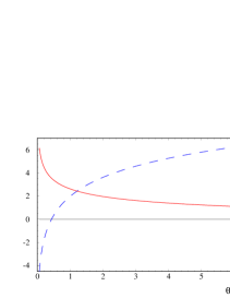
Figure 1: Logarithmically enhanced (dashed line) and nonlogarithmic (solid line) second order corrections to the differential cross section of the small angle Bhabha scattering as functions of the scattering angle for $\sqrt{s}=100$ GeV and $\ln(\varepsilon_{cut}/\varepsilon)=0$, in units of $10^{-3}$.

The second order corrections to the differential cross section $(\alpha/\pi)^{2}{\rm d}\sigma^{(2)}/{\rm d}\sigma^{(0)}$ are plotted as functions of the scattering angle for the small angle Bhabha scattering at $\sqrt{s}=100$ GeV on Fig. (1) and for the large angle Bhabha scattering at $\sqrt{s}=1$ GeV on Fig. (2). We separate the logarithmically enhanced corrections given by the first two terms of Eq. (2) and nonlogarithmic contribution given by the last term of this equation. All the terms involving a power of the logarithm $\ln(\varepsilon_{cut}/\varepsilon)$ are excluded from the numerical estimates because the corresponding contribution critically depends on the event selection algorithm and cannot be unambiguously estimated without imposing specific cuts on the photon bremsstrahlung. We observe that for scattering angles $\theta\mbox{\raisebox{-3.0pt}{$\stackrel{{\scriptstyle<}}{{\sim}}$}}18^{o}$ and $\theta\mbox{\raisebox{-3.0pt}{$\stackrel{{\scriptstyle>}}{{\sim}}$}}166^{o}$ the nonlogarithmic contribution exceeds $0.05\%$, and in the low energy case exceeds the logarithmically enhanced contribution for $\theta\mbox{\raisebox{-3.0pt}{$\stackrel{{\scriptstyle<}}{{\sim}}$}}8^{o}$.

To conclude, we have derived the two-loop radiative photonic corrections to Bhabha scattering in the leading order of the small electron mass expansion up to nonlogarithmic term. The nonlogarithmic contribution has been found numerically important for the practically interesting range of scattering angles. Together with the result of Refs. BFMR ; Bon for the corrections with the closed fermion loop insertions our result gives a complete expression for the two-loop virtual corrections. It should be incorporated into the Monte Carlo event generators to reduce the theoretical error in the luminosity determination at present and future electron-positron colliders below $0.1\%$.

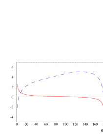
Figure 2: The same as Fig. (1) but for the large angle Bhabha scattering and $\sqrt{s}=1$ GeV.

- (1) S. Jadach et al. in G. Altarelli, T. Sjöstrand and F. Zwirner (eds.), Physics at LEP2, CERN-96-01, hep-ph/9602393; G. Montagna, O. Nicrosini, and F. Piccinini, Riv. Nuovo Cim. 21N9, 1 (1998).
- (2) N. Toomi, J. Fujimoto, S. Kawabata, Y. Kurihara, and T. Watanabe, Phys. Lett. B 429, 162 (1998); R.D. Heuer, D. Miller, F.Richard, and P.M. Zerwas, (eds.), TESLA Technical design report. Pt. 3: Physics at an linear collider, DESY-01-011C.
- (3) C. M. Carloni Calame, C. Lunardini, G. Montagna, O. Nicrosini, and F. Piccinini, Nucl. Phys. B584, 459 (2000).
- (4) M. Bohm, A. Denner, and W. Hollik, Nucl. Phys. B304, 687 (1988).
- (5) Z. Bern, L. Dixon, and A. Ghinculov, Phys. Rev. D 63, 053007 (2001).
- (6) R. Bonciani, A. Ferroglia, P. Mastrolia, and E. Remiddi, Nucl. Phys. B701, 121 (2004).
- (7) R. Bonciani, A. Ferroglia, P. Mastrolia, E. Remiddi, and J.J. van der Bij, Nucl. Phys. B716, 280 (2005).
- (8) V.A. Smirnov, Phys. Lett. B 524, 129 (2002); Nucl. Phys. Proc. Suppl. 135, 252 (2004); G. Heinrich and V.A. Smirnov, Phys. Lett. B 598, 55 (2004); M. Czakon, J. Gluza, and T. Riemann, Nucl. Phys. Proc. Suppl. 135, 83 (2004); Report No. DESY 04-222 and hep-ph/0412164.
- (9) A.B. Arbuzov, V.S. Fadin, E.A. Kuraev, L.N. Lipatov, N.P. Merenkov, and L. Trentadue, Nucl. Phys. B485, 457 (1997).
- (10) A.B. Arbuzov, E.A. Kuraev, and B.G. Shaikhatdenov, Mod. Phys. Lett. A 13, 2305 (1998)
- (11) E.W. Glover, J.B. Tausk, and J.J. van der Bij, Phys. Lett. B 516, 33 (2001).
- (12) T. Kinoshita, J. Math. Phys. 3, 650, (1962); T.D. Lee and M. Nauenberg, Phys. Rev. B 133, 1549 (1964).
- (13) G. Sterman and S. Weinberg, Phys. Rev. Lett. 39, 1436 (1977)
- (14) V.A. Smirnov, Applied Asymptotic Expansions in Momenta and Masses (Springer-Verlag, Heidelberg, 2001).
- (15) B. Feucht, J.H. Kühn, A.A. Penin, and V.A. Smirnov, Phys. Rev. Lett. 93, 101802 (2004).
- (16) D.R. Yennie, S.C. Frautschi, and H. Suura, Ann. Phys. 13, 379 (1961). A.H. Mueller, Phys. Rev. D 20, 2037 (1979); J.C. Collins, Phys. Rev. D 22 (1980) 1478; A. Sen, Phys. Rev. D 24, 3281 (1981); 28, 860 (1983); G. Sterman, Nucl. Phys. B281, 310 (1987); V.S. Fadin, L.N. Lipatov, A.D. Martin and M. Melles, Phys. Rev. D 61, 094002 (2000); J.H. Kühn, A.A. Penin, and V.A. Smirnov, Eur. Phys. J. C 17, 97 (2000); Nucl. Phys. Proc. Suppl. 89, 94 (2000).
- (17) J. Frenkel and J.C. Taylor, Nucl. Phys. B116, 185 (1976).
- (18) J.H. Kühn, S. Moch, A.A. Penin, and V.A. Smirnov, Nucl. Phys. B616, 286 (2001); B648, 455(E) (2003).
- (19) S. Catani, Phys. Lett. B 427, 161 (1998).
- (20) G. Kramer and B. Lampe, Z. Phys. C 34, 497 (1987); 42, 504(E) (1989); T. Matsuura, S.C. van der Marck and W.L. van Neerven, Nucl. Phys. B 319, 570 (1989).
- (21) P. Mastrolia and E. Remiddi, Nucl.Phys. B664, 341 (2003).
- (22) R. Barbieri, J.A. Mignaco, and E. Remiddi, Nuovo Cim. A 11, 824 (1972).
- (23) G.J.H. Burgers, Phys. Lett. B 164, 167 (1985).
- (24) V.S. Fadin, E.A. Kuraev, L.N. Lipatov, N.P. Merenkov, and L. Trentadue, Fhys. Atom. Nucl. 56, 1537 (1993) [Yad. Fiz. 56 145 (1993)].
- (25) R. Bonciani and A. Ferroglia, Report No. FREIBURG-THEP-05-06 and hep-ph/0507047.