$\pi\pi$ scattering, pion form factors and chiral perturbation theory

Abstract

I discuss recent progress in our understanding of the $\pi\pi$ scattering amplitude at low energy thanks to the combined use of chiral perturbation theory and dispersion relations. I also comment on the criticism raised by Peláez and Ynduráin on this work.

1 Introduction

In the previous conference of this series I was invited to present results Colangelo:2002tn concerning the experimental determination of the $\bar{q}q$ condensate in the SU(2) chiral limit Colangelo:2001sp , based on an analysis of the Brookhaven E865 data Pislak:2003sv on the low-energy $\pi\pi$ phase shift as extracted from $K_{e4}$ decays. These experimental results and their analysis closed a long-standing discussion about the size of this order parameter of chiral symmetry breaking in QCD (cf. Descotes-Genon:2001tn and references therein): the scenario in which the SU(2) $\bar{q}q$ condensate is unexpectedly small, or even vanishing, though interesting, is now experimentally excluded. Only the dependence of this condensate on the number of massless flavours still remains an open issue (cf. Descotes-Genon:2002yv and references therein). In the yet earlier conference Colangelo:2000fd , within a general discussion of recent progress in chiral perturbation theory (CHPT), I had already presented our predictions for the two $S$-wave scattering lengths Colangelo:2000jc .

This work on $\pi\pi$ scattering has a few features which are worth stressing:

• the precision reached (at the level of a few percent) is quite unusual for hadronic physics;

• this precision concerns a prediction – experiments have not yet reached the same level of accuracy (“theory is ahead of experiment” as Heiri Leutwyler puts it Leutwyler:2002hk );

• despite a rather heavy machinery which is necessary to obtain this prediction, the latter does follow from QCD, and indeed the experimental tests tell us something about QCD, as the conclusion about the size of the $\bar{q}q$ condensate shows.

The precision obtained in our theoretical understanding of the $\pi\pi$ scattering amplitude at low energy is not only important per se, but has also important consequences for a number of other processes. In almost every low energy hadronic process the interaction among pions plays an important role, and being able to treat this accurately may lead to relevant improvements. An example of this is the anomalous magnetic moment of the muon, where one can make good use of the accurate knowledge of the $\pi\pi$ $P$-wave phase shift Colangelo:2003yw .

An essential role in this improved understanding of the $\pi\pi$ scattering amplitude at low energy has been played by the combined use of CHPT and dispersion relations. In CHPT, even after a two-loop calculation of the $\pi\pi$ scattering amplitude, one finds out that only close to the center of the Mandelstam triangle the series converges rather fast, whereas at threshold the convergence is surprisingly slow: a direct evaluation of the scattering lengths in CHPT would not have reached the same precision level 2lpipi . On the other hand a purely dispersive analysis of $\pi\pi$ scattering, as performed in the seventies (for a review of this early work cf. pennington ) using Roy equations Roy did not lead to precise predictions either, because of lack of information on the subtraction constants. If one uses CHPT to pin down the latter, the scheme becomes predictive and accurate. In our work we first had to redo the Roy equation analysis Ananthanarayan:2000ht and then matched the dispersive representation to the chiral one Colangelo:2001df .

Some of the input used in the Roy equation analysis in Ananthanarayan:2000ht has been criticised by Peláez and Ynduráin Pelaez:2003eh , and doubts have been cast on the level of precision reached in our analysis. This criticism has been immediately answered Caprini:2003ta . Also, the more recent objections raised in Yndurain:2003vk on the dispersive determination of the scalar radius discussed in Colangelo:2001df were shown to be unfounded Ananthanarayan:2004xy .

In the present edition of the conference a session has been devoted to a discussion of these issues. In this contribution I will present my view on these issues and on the ongoing discussion – of course, the current view of Peláez and Ynduráin can also be found in these proceedings Pelaez:2004xx . Rather then concentrating on the reply to the criticism raised by Peláez and Ynduráin, which is rather technical and can anyway be found in the original papers Caprini:2003ta ; Ananthanarayan:2004xy , I will review the work we did on the $\pi\pi$ scattering amplitude and discuss its importance also in view of future experimental tests, as well as tests and comparisons with lattice calculations. I will also briefly discuss the criticism and our reply, but I wish to stress right away that the points raised in Pelaez:2003eh have all been answered in Caprini:2003ta , and that the claimed violation of a “robust lower bound” Yndurain:2003vk in our calculation of the scalar radius has been shown to be a non-issue because this lower bound does not exist Ananthanarayan:2004xy . The discussion on these issues is closed. In a more recent paper Pelaez:2004xy Peláez and Ynduráin claim that our representation for the $\pi\pi$ scattering amplitude fails to satisfy some dispersion relations. We have not yet evaluated these, and I can therefore not comment on this claimed failure. Moreover, in their contribution to these proceedings they criticize our choice of one of the input parameters in our Roy analysis, the value of the $S$-wave isoscalar phase shift at $0.8$ GeV – I will comment on this point below.

2 $\pi\pi$ scattering: Roy equations and CHPT

In SU(2) CHPT the expansion parameter is $\hat{m}/M_{\rho}$ and one expects higher order corrections to be of the order of a few percents. There are many known examples in which this naive expectation is violated and corrections are substantially larger. A well known example is the $\pi\pi$ $S$-wave isoscalar scattering length which has been first evaluated by Weinberg Weinberg:1966xx to leading order in the chiral expansion. Numerically this gives $a_{0}^{0}(\mathrm{LO})=0.16$, but the next-to-leading order corrections, first calculated by Gasser and Leutwyler Gasser:1984xx shift this value by about 25%, $a_{0}^{0}(\mathrm{NLO})=0.20$. The next-to-next-to-leading order corrections have also been evaluated 2lpipi and have been found to be not yet negligible, shifting the value by another 10% up to $a_{0}^{0}(\mathrm{NNLO})=0.22$. The error estimate for this quantity is not trivial: first of all one has to determine a number of low-energy constants (LEC) which appear in the chiral expansion of this quantity and estimate the corresponding error. Second, one has to estimate the size of yet higher order corrections. At first sight going below the 10% level for the total error appears to be difficult. The reason for the large size of the higher order corrections for this quantity, however, is well understood and is due to the strong interaction of the pions in the $I=0$ $S$ wave: the perturbative expansion for these unitarity corrections converges slowly. In a dispersive framework, on the other hand, these unitarity corrections can be treated exactly.

If one combines the dispersive and the chiral approaches one can make a quantum jump in accuracy: the dispersive treatment can be used to evaluate the unitarity corrections which are problematic in the chiral expansion, and CHPT can be used to fix the subtraction constants which represent the only true degrees of freedom in the dispersive treatment at low energy. The crucial point is that if one chooses the subtraction constants properly, the chiral expansion for these does indeed follow the naive expectations about the size of the higher order corrections. Moreover, in the low energy region, the dispersive treatment does lead to very precise results.

I will now illustrate in some more detail this program and first discuss the Roy equations and their numerical solution and then the matching to the chiral representation and the numerical prediction for the scattering lengths.

2.1 Roy equations

In 1971 Roy Roy showed that using crossing one can write a set of dispersion relations for the $\pi\pi$ scattering amplitude which involve only physical region singularities. When projected onto partial waves these equations take the form of an infinite set of integral equations in which the real part of any partial wave is given by an integral over the imaginary parts of all partial waves in the physical region. At low energy (say below 1 GeV) the $S$ and $P$ waves dominate, and it suffices to consider the equations only for these lowest partial waves. For example, the Roy equation for the $S$, $I=0$ wave reads as follows

$$\mbox{Re}\,t_{0}^{0}(s) = k_{0}^{0}(s)+-\int_{4M_{\pi}^{2}}^{E_{0}^{2}}ds^{\prime}K_{0\,0}^{0\,0}(s,s^{\prime})\,\mbox{Im}\,t_{0}^{0}(s^{\prime})+-\int_{4M_{\pi}^{2}}^{E_{0}^{2}}ds^{\prime}K_{0\,1}^{0\,1}(s,s^{\prime})\,\mbox{Im}\,t_{1}^{1}(s^{\prime})$$ (1)

$$+ -\int_{4M_{\pi}^{2}}^{E_{0}^{2}}ds^{\prime}K_{0\,0}^{0\,2}(s,s^{\prime})\,\mbox{Im}\,t_{0}^{2}(s^{\prime})+f_{0}^{0}(s)+d_{0}^{0}(s)\;\;,$$

where $k_{0}^{0}$ is the contribution of the subtraction polynomial, $f_{0}^{0}$ the contribution from the intermediate energy region and $d_{0}^{0}$ the so-called driving term containing both the contribution from the high-energy region as well as that from the higher partial waves:

$$k^{0}_{0}(s) = a_{0}^{0}+\frac{s-4M_{\pi}^{2}}{12M_{\pi}^{2}}\,(2a_{0}^{0}-5a_{0}^{2})$$

$$f_{0}^{0}(s) = \sum_{I^{\prime}=0}^{2}\sum_{\ell^{\prime}=0}^{1}-\int_{E_{0}^{2}}^{E_{1}^{2}}ds^{\prime}K_{0\ell^{\prime}}^{0I^{\prime}}(s,s^{\prime})\,\mbox{Im}\,t_{\ell^{\prime}}^{I^{\prime}}(s^{\prime})$$

$$d_{0}^{0}(s) = \mbox{all the rest}\;\;.$$ (2)

The two energies $E_{0,1}$ were chosen in Ananthanarayan:2000ht to be $E_{0}=0.8$ GeV and $E_{1}=2$ GeV. With this choice of $E_{0}$ the solution has been shown to be unique Gasser:1999hz . The $f_{0}^{0}$ term is evaluated using the imaginary parts Im$t^{I}_{\ell}$ measured in $\pi N\to\pi\pi N$ experiments, whereas the driving terms are evaluated using experimental information on the lowest lying resonances in $D$ and higher partial waves, and Regge representations for the high-energy $\pi\pi$ scattering amplitude. The kernels $K_{II^{\prime}}^{\ell\ell^{\prime}}(s,s^{\prime})$ are all known explicitly Ananthanarayan:2000ht .

The upshot of the analysis in Ananthanarayan:2000ht is that if the input above $E_{0}$ is given, the solution of the equations below $E_{0}$ is uniquely fixed by the two scattering lengths $a_{0}^{0}$ and $a_{0}^{2}$. Actually only one of the two is a true free parameter if the solution has to be physical, i.e. if it has no cusps at $E_{0}$. Since the input above $E_{0}$ is not known with infinite accuracy, this correlation among the two input parameters is not a line, but gets broadened into a band known as the Universal Band. A similar correlation among the two scattering lengths is also given by the Olsson sum rule Olsson .

2.2 Matching the chiral and the dispersive representation

In the early literature on Roy equations the subtraction constants were taken as free parameters – in the region below the matching point $E_{0}$ these were the main sources of uncertainty and it was difficult to turn the Roy equation machinery into a predictive scheme. The best use one could make of Roy equation solutions was to analyze data in the low-energy region, like those from $K_{e4}$ decays, in order to determine the scattering lengths – in much the same way as the E865 collaboration Pislak:2003sv has used our Roy equation solutions Ananthanarayan:2000ht . The point of view has changed drastically once it has become clear that CHPT can provide rather accurate predictions for the scattering lengths Gasser:1984xx .

As mentioned above, however, the scattering lengths are not the quantities that CHPT can most accurately predict. Since the choice of the subtraction point is arbitrary, one can exploit this freedom and subtract below threshold, close to the center of the Mandelstam triangle, in order to be far from the singularities that make the chiral series converge slowly. By doing so one can optimize the accuracy of the whole scheme as is well illustrated by the following breakdown of $a_{0}^{0}$ into various contributions:

$$a^{0}_{0}=\frac{7M_{\pi}^{2}}{32\pi F_{\pi}^{2}}\,C_{0}+M_{\pi}^{4}\,\alpha_{0}+O(M_{\pi}^{8})$$ (3)

where

$$C_{0}=1+\frac{M_{\pi}^{2}}{3}\,\langle r^{2}\rangle\rule[-1.99997pt]{0.0pt}{0.0pt}_{s}-\frac{5\,M_{\pi}^{2}}{224\pi^{2}F_{\pi}^{2}}\left\{\bar{\ell}_{3}-\frac{563}{525}\right\}+O(M_{\pi}^{4})$$ (4)

(here given only at next-to-leading order, for simplicity) is the part of the scattering length which only depends on the quark masses, whereas $\alpha_{0}$ is the part which is due to the momentum dependent part of the amplitude, here evaluated at threshold.

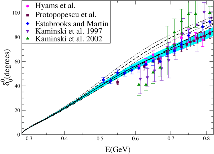
Figure 1: Phase shift for the $I=0$ $S$ wave. The shaded band is the result of the analysis in Colangelo:2001df and the solid line is the Roy equation solution obtained with the input above $1.4$ GeV proposed in Pelaez:2003eh . The dashed curve and the corresponding uncertainty band are the “tentative alternate solution” proposed in Pelaez:2003eh . The dotdashed curve is the Roy solution fit to the Kaminski et al. 1997 KLR data obtained in Kaminski:2002pe . The other data sets shown are from Refs. hyams ; proto ; EM

The constant $C_{0}$ is to be chosen as subtraction constant in the dispersive treatment, because for this the chiral expansion converges fast: the numerical evaluation at the two-loop level gives

$$C_{0}=1.096\pm 0.021$$ (5)

amounting to a 10% shift evaluated with 20% of relative uncertainty. This correction shifts $a_{0}^{0}$ from $0.16$ to $0.17$. The bulk of the correction, however, comes from the momentum dependent part of the amplitude, the $\alpha_{0}$ term which can be accurately evaluated through a dispersive integral. The final result for both $S$-wave scattering lengths reads

$$a_{0}^{0}=0.220\pm 0.005\qquad a_{0}^{2}=-0.0444\pm 0.0010\;\;,$$ (6)

with an accuracy at the level of a few percent for both. Notice that the situation is completely different for $a^{2}_{0}$: here the tree level result is $-0.0454$ and the momentum-dependent part of the correction is not particularly large. As is well known the $\pi\pi$ interaction in the $I=2$ channel is weak.

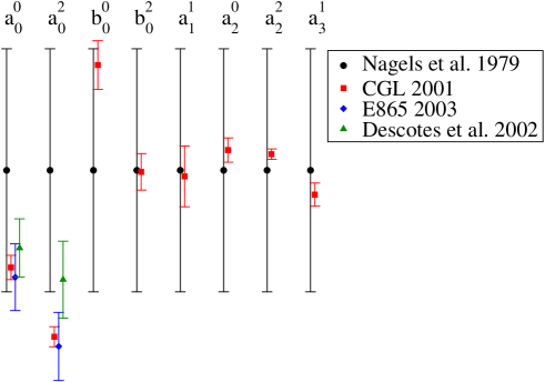
Figure 2: Accuracy improvement in the evaluation of various threshold parameters due to the use of CHPT for the subtraction constants.

If one uses the dispersive representation for the $\pi\pi$ scattering amplitude, this high level of accuracy obtained for the scattering lengths is reflected in the whole energy region below $E_{0}$: having fixed the scattering lengths all other sources of noise generate remarkably little uncertainty as illustrated for the case of the $S0$ wave in Fig. 1. Notice that the band is a prediction which relies on experimental input only at $0.8$ GeV and above – it is not a fit to any of the data sets shown in the same plot. The plot contains various data sets as well as the “tentative alternate solution” proposed by Peláez and Ynduráin in Pelaez:2003eh and the Roy solution fit of Kaminski et al. Kaminski:2002pe . These will be commented upon in the next section. That CHPT is mostly responsible for the improvement in the accuracy in the Roy treatment is well illustrated in Fig. 2, where the values for a number of threshold parameters obtained from Roy equation analyses as reported in the compilation of data Nagels are given in arbitrary units chosen such that all errors are normalized to the same size. The errors obtained after matching the dispersive and the chiral representation are about an order of magnitude smaller.

3 The criticism of Peláez and Ynduráin

In Pelaez:2003eh Peláez and Ynduráin have criticized our work Ananthanarayan:2000ht ; Colangelo:2001df and made the following claims: that the input used in the Roy equation analysis above 1.4 GeV was incorrect and that as a consequence the solutions we obtained below 0.8 GeV were also incorrect. The claim about the incorrectness of the input has two aspects: between 1.4 GeV and 2 GeV we used experimental information and they claim that this is unreliable – above 2 GeV, where we relied on a Regge representation, they claimed that the one we used is not orthodox because it does not respect factorization. According to the latter property, the residues of the Regge poles which appear in the $\pi\pi$ scattering amplitude must be given by the square of the residue for $\pi N$ divided by the $NN$ residue. As explicitly stated in Ananthanarayan:2000ht the Regge representation we used served the purpose of giving us a fair account of the contributions to the dispersive integrals from the regions between 2 and 3 GeV – the contributions from yet higher energies are negligible because the Roy equations are twice subtracted. In fact even the contributions from the region above 1.4 GeV are rather small and play a minor role in the Roy equations. For this reason we have not made our own analysis of this part of the input and took what was available in the literature.

The observation that contributions from above 1.4 GeV do not matter much for the Roy solutions below 0.8 GeV appears to be in contradiction with the second claim made by Peláez and Ynduráin, namely that the solutions we obtained were “spurious” because of the incorrect input used. It is important to stress here that Peláez and Ynduráin made this claim without supporting it with a calculation, but only with indirect arguments. I will come back to these indirect arguments later but I first must say that the Roy equation solutions for the input proposed by Peláez and Ynduráin as the correct one have been calculated in Caprini:2003ta . The outcome is the solid line in Fig. 1 and is indistinguishable from the solution obtained with the input originally used in Ananthanarayan:2000ht . The calculation shows that the second claim of Peláez and Ynduráin is wrong.

This takes us back to the indirect arguments they had used to support their claim. They gave three arguments:

1. a mismatch in the Olsson sum rule;

2. a discrepancy among two different determinations of the $P$-wave effective range;

3. a discrepancy among two different evaluations of the $D$ and $F$ wave threshold parameters.

In Caprini:2003ta we have discussed in detail all these indirect arguments and shown that either the discrepancy is not there (as in the case of the $P$ wave effective range) or that the conclusion that the discrepancy can be cured by changing the Roy solution below 0.8 GeV is incorrect. The interested reader is referred to Caprini:2003ta for a detailed discussion of all these points.

As explicitly stated also in Caprini:2003ta , a better input than the Regge representation that we have used in Ananthanarayan:2000ht is certainly possible and can obtained with a thorough analysis of all the available information (like high-energy total cross section data, sum rules etc.) Caprini-WIP . In this perspective, also the data on total $\pi\pi$ cross sections which Peláez and Ynduráin have pointed out Pelaez:2004xx are useful information which has to be taken into account – the representation used in Ananthanarayan:2000ht does not describe these very well and can be improved. It is however a fact that the influence of improvements in the high-energy input on the scattering lengths and the whole low-energy scattering amplitude will be negligible. Such improvements may be of interest in applications which rely on the $\pi\pi$ scattering amplitude close to $1$ GeV, like the dispersive representation of hadronic contributions to $a_{\mu}$ which relies on the $P$ wave phase shifts Colangelo:2003yw .

3.1 The input phase $\delta_{0}^{0}(0.8\mbox{GeV})$

In the most recent papers Peláez and Ynduráin have moved on to discuss other points and to raise further criticism to our analysis. In particular they have criticized our value and error for $\delta_{0}^{0}(E_{0})$ which, as discussed at length in Ananthanarayan:2000ht , is one of the most important input parameters in the Roy analysis.

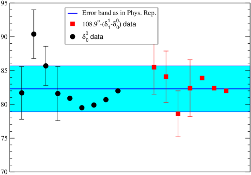
Figure 3: Graphical representation of the data on $\delta_{0}^{0}(0.8\mbox{GeV})$ as given in Table 2, p. 226 of Ref. Ananthanarayan:2000ht : on the left-hand side of the plot the plain data for $\delta_{0}^{0}(0.8\mbox{GeV})$ are shown. On the right-hand side those for the difference $\delta_{0}^{0}(0.8\mbox{GeV})-\delta_{1}^{1}(0.8\mbox{GeV})$ shifted by $108.9^{\circ}$, the value of the $P$ wave phase shift as extracted from form factor data.

In this paper we had observed that if one looks at the data on this particular wave it is difficult to draw any conclusion because different data sets (in fact different analyses of the same $\pi N\to\pi\pi N$ scattering data) are mutually incompatible. The situation improves dramatically if one looks at the difference $\delta_{1}^{1}(E_{0})-\delta_{0}^{0}(E_{0})$, for which different data sets give a coherent picture. The fact that the $\delta_{1}^{1}$ phase is now known much better thanks to the data on the vector form factor then leads to a rather good determination of $\delta_{0}^{0}(E_{0})$ which we estimated to be $82.3^{\circ}\pm 3.4^{\circ}$. This is illustrated in Fig. 3 which compares the direct determinations of $\delta_{0}^{0}(E_{0})$ to those that exploit the phase difference. In their recent discussions Peláez and Ynduráin have given particular emphasis to the recent analyses by Kaminski et al. KLR . This is indeed important new work on $\pi\pi$ scattering because it analyzes a large body of polarized $\pi N\to\pi\pi N$ data, which are certainly very interesting and useful. The data of these two analyses are shown in Fig. 1: around 0.8 GeV these data are substantially higher than those of Hyams et al. or Protopopescu et al. and our band. In that region the “tentative alternate solution” proposed by Peláez and Ynduráin in Pelaez:2003eh is in better agreement with them. Below 0.7 GeV, however, the Kaminski et al. data become lower than the other data sets and also lower than the two bands shown: even the “tentative alternate solution” is now in flat disagreement with these data. The problem is seen also in a recent paper by Kaminski et al. Kaminski:2002pe where they solve Roy equations and fit the data with the solutions: the overall fit is not particularly good precisely because this peculiar shape of the data in this energy region (low between 0.6 and 0.7 GeV, rising steeply at 0.7 GeV and then high until 0.8 GeV) cannot be followed by Roy equation solutions. This best fit to their data is shown in Fig. 1 as dotdashed curve, and is evidently a trade-off between the high and the low data. This curve lies almost everywhere inside our Roy solution band and has $\delta_{0}^{0}(0.8\mbox{GeV})=87^{\circ}$, about 1.5 $\sigma$ higher than the range we had used as input.

This most recent analysis does not clarify the experimental situation concerning the $S0$ wave. Since no information is provided on the phase difference $\delta_{1}^{1}-\delta_{0}^{0}$ we could not make use of these data when we fixed the input for the Roy equations. Moreover the results of the Roy equation analysis of Kaminski et al. Kaminski:2002pe we just discussed show that there is no reason to modify our central value for $\delta_{0}^{0}(0.8\mbox{GeV})$ or to stretch its error.

3.2 Scalar radius

Another point on which criticism has been raised against our analysis concerns the scalar radius $\langle r^{2}\rangle\rule[-1.99997pt]{0.0pt}{0.0pt}_{s}$ which appears in the chiral expansion of both $S$-wave scattering lengths, cf. Eq. (4). The input value we used Colangelo:2001df :

$$\langle r^{2}\rangle\rule[-1.99997pt]{0.0pt}{0.0pt}_{s}=0.61\pm 0.04\mathrm{fm}^{2}$$ (7)

had been determined through a dispersive analysis of the scalar form factor, following Donoghue:1990xh after updating the $\pi\pi$ phase shifts which are used as input. Ynduráin has recently claimed that the outcome of this calculation violates a “robust lower bound” he derives Yndurain:2003vk . The same bound is violated also by other calculations of the same quantity. One of them, performed by Moussallam Moussallam:1999 , makes a thorough analysis of the different phenomenological inputs available in the literature and comes to a conclusion which is in perfect agreement with Eq. (7): the values he finds for the radius lie between $0.58$ and $0.65\,\mbox{fm}^{2}$.

This apparent puzzle has been recently clarified in Ananthanarayan:2004xy : the “robust lower bound” does not exist because its derivation relies on an untenable assumption, namely that the phase of the scalar form factor in the region above $1.1$ GeV must be close to the $S0$ phase shift. The correct conclusion is that above $1.1$ GeV where the elasticity is again close to one, the difference between the phase of the scalar form factor and the phase shift has to be close to a multiple of $\pi$: the various available calculations all agree that this difference is close to $\pi$ rather than to zero. Also this criticism is unjustified.

4 Outlook

The predictions for the $S$ wave $\pi\pi$ scattering lengths (6) discussed here are of unusual precision in hadronic physics. They are derived under the assumption that the quark condensate is the leading order parameter of the spontaneous symmetry breaking in QCD. Experimental tests have confirmed this hypothesis and have put the standard picture of the QCD vacuum on a solid experimental basis. The predictions are however still more precise than the experimental measurements of the same quantities, and there is still room for a more stringent test of QCD at low energy. Experiments aiming at performing these tests are currently underway: the DIRAC experiment at CERN DIRAC is measuring the lifetime of pionic atoms which is proportional to the square of the difference of the two scattering lengths and plans to reach a 5% precision in the measurement of this difference. The NA48II experiment NA48II will gather twice the statistics of $K_{e4}$ decays of the E865 experiment, thus reaching an improvement of a factor $\sqrt{3}$ in the final uncertainty. The phase shift difference measured in these decays is mostly sensitive to $a_{0}^{0}$. The prospects for precision low-energy hadronic physics are at the moment particularly good. We look forward to the experimental results.

References

- (1) G. Colangelo, Proc. of the 5th International Conference on Quark Confinement and the Hadron Spectrum, Gargnano, Italy, 10-14 Sep 2002
- (2) G. Colangelo, J. Gasser and H. Leutwyler, Phys. Rev. Lett. 86 (2001) 5008 [arXiv:hep-ph/0103063].
- (3) S. Pislak et al., Phys. Rev. D 67 (2003) 072004 [arXiv:hep-ex/0301040].
- (4) S. Descotes-Genon, N. H. Fuchs, L. Girlanda and J. Stern, Eur. Phys. J. C 24 (2002) 469 [arXiv:hep-ph/0112088].
- (5) S. Descotes-Genon, L. Girlanda and J. Stern, Eur. Phys. J. C 27 (2003) 115 [arXiv:hep-ph/0207337].
- (6) G. Colangelo, arXiv:hep-ph/0011025.
- (7) G. Colangelo, J. Gasser and H. Leutwyler, Phys. Lett. B 488 (2000) 261 [arXiv:hep-ph/0007112].
- (8) H. Leutwyler, AIP Conf. Proc. 670 (2003) 45 [arXiv:hep-ph/0212323].
- (9) G. Colangelo, arXiv:hep-ph/0312017.
-
(10)
M. Knecht, B. Moussallam, J. Stern and N. H. Fuchs,
Nucl. Phys. B 457 (1995) 513
[arXiv:hep-ph/9507319],
and Nucl. Phys. B 471 (1996) 445
[arXiv:hep-ph/9512404].
J. Bijnens, G. Colangelo, G. Ecker, J. Gasser and M. E. Sainio, Phys. Lett. B 374 (1996) 210 [arXiv:hep-ph/9511397], and Nucl. Phys. B 508 (1997) 263 [Err.-ibid. B 517 (1998) 639] [arXiv:hep-ph/9707291]. - (11) M. R. Pennington, Annals Phys. 92 (1975) 164.
- (12) S. M. Roy, Phys. Lett. B 36 (1971) 353.
- (13) B. Ananthanarayan, G. Colangelo, J. Gasser and H. Leutwyler, Phys. Rept. 353 (2001) 207 [arXiv:hep-ph/0005297].
- (14) G. Colangelo, J. Gasser and H. Leutwyler, Nucl. Phys. B 603 (2001) 125 [arXiv:hep-ph/0103088].
- (15) J. R. Pelaez and F. J. Yndurain, Phys. Rev. D 68 (2003) 074005 [arXiv:hep-ph/0304067].
- (16) I. Caprini, G. Colangelo, J. Gasser and H. Leutwyler, Phys. Rev. D 68 (2003) 074006 [arXiv:hep-ph/0306122].
- (17) F. J. Yndurain, Phys. Lett. B 578 (2004) 99 [Err.-ibid. B 586 (2004) 439] [arXiv:hep-ph/0309039].
- (18) B. Ananthanarayan et al. Phys. Lett. B 602 (2004) 218 [arXiv:hep-ph/0409222].
- (19) J. R. Pelaez and F. J. Yndurain arXiv:hep-ph/0411334.
- (20) J. R. Pelaez and F. J. Yndurain arXiv:hep-ph/0412320, these proceedings.
- (21) S. Weinberg Phys. Rev. Lett. 17 (1966) 616.
- (22) J. Gasser and H. Leutwyler, Phys. Lett. B 125 (1983) 325, and Annals Phys. 158 (1984) 142.
- (23) J. Gasser and G. Wanders, Eur. Phys. J. C 10 (1999) 159 [arXiv:hep-ph/9903443].
- (24) M. G. Olsson, Phys. Lett. B410 (1997) 311 [hep-ph/9703247].
-
(25)
R. Kaminski, L. Lesniak and K. Rybicki,
Z. Phys. C 74 (1997) 79
[arXiv:hep-ph/9606362],
Eur. Phys. J. directC 4 (2002) 4 [arXiv:hep-ph/0109268]. - (26) R. Kaminski, L. Lesniak and B. Loiseau, Phys. Lett. B 551 (2003) 241 [arXiv:hep-ph/0210334].
- (27) B. Hyams et al., Nucl. Phys. B64 (1973) 134.
- (28) S. D. Protopopescu et al., Phys. Rev. D7 (1973) 1279.
- (29) P. Estabrooks and A. D. Martin, Nucl. Phys. B79 (1974) 301.
- (30) M. M. Nagels et al., Nucl. Phys. B 147 (1979) 189.
- (31) I. Caprini, G. Colangelo and H. Leutwyler, work in progress.
- (32) J. F. Donoghue, J. Gasser and H. Leutwyler, Nucl. Phys. B 343 (1990) 341.
- (33) B. Moussallam, Eur. Phys. J. C 14 (2000) 111 [arXiv:hep-ph/9909292].
- (34) Preliminary results can be found at http://dirac.web.cern.ch/DIRAC/.
- (35) See: http://na48.web.cern.ch/NA48/NA48-2/NA48_2.html