Supersymmetry at LHC and ILC

Abstract

The prospects for the discovery and exploration of low-energy Supersymmetry at future colliders, the Large Hadron Collider (LHC) and the future international linear electron positron collider (ILC) are summarized. The focus is on the experimental techniques that will be used to discover superpartners and to measure their properties. Special attention is given to the question how the results from both machines could influence each other, in particular when they have overlapping running time.

I INTRODUCTION

The search for SUSY and, should it be found, measurements of the superpartner properties are among the most important motivations for future high energy particle colliders. A general introduction to TeV-scale Supersymmetry (SUSY) as one of the best motivated extensions of the Standard Model (SM) has been given elsewhere in these proceedings tata . The Large Hadron Collider (LHC) currently under construction at CERN will go into operation in 2007 and has a huge potential for SUSY discovery as well as for first measurements of SUSY particle properties. The planned International Linear electron positron Collider (ILC) is an ideal tool for precision SUSY measurements. Both machines together will be able to give important insight into the mechanism of SUSY breaking and may open a window to GUT/Planck scale physics.

In this article, in Section II the prospects for inclusive SUSY discovery at the LHC are summarized. Furthermore studies for the exclusive reconstruction of superpartners and the measurement of their masses are explained. In Section III the prospects for precision SUSY measurements at the ILC are shown. The different techniques for mass measurements, measurements of polarized cross-sections and quantum numbers of the superpartners are detailed with some explicit examples. Finally, in Section IV the interplay of the anticipated results of both LHC and and ILC in particular when analyzed simultaneously is shown. The extended Higgs-sector of supersymmetric models also is an integral part of future exploration of SUSY. The prospects for Higgs searches and precision measurements at LHC and ILC are summarized elsewhere in these proceedings albert .

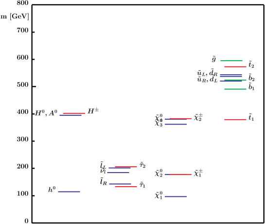
Figure 1: SUSY mass spectrum for the mSUGRA benchmark point SPS1a sps1a .

II SUSY AT THE LHC

II.1 Experimental environment

The LHC will produce proton-proton collisions at a center-of-mass energy of 14 TeV initially at a luminosity of $1\times 10^{33}{\rm cm}^{-2}{\rm s}^{-1}$ (low-luminosity) and later at $1\times 10^{34}{\rm cm}^{-2}{\rm s}^{-1}$ (high luminosity). The high center-of-mass energy makes this machine well suited for the direct discovery of new massive particles beyond the SM. The partonic luminosity is large enough to pair-produce colored new particles (like squarks and gluinos) up to masses of a few TeV at observable rates. The high luminosity and the large total pp cross-section impose strong requirements on the performance of the detectors and in particular on the trigger. The two multi-purpose detectors, ATLAS ATLAS and CMS CMS , will be able to trigger efficiently on high-$p_{T}$ leptons, jets and are due to their hermeticity sensitive to missing transverse energy. Thus they are well suited for the typical experimental signatures of SUSY. The hadronic environment, however makes the exclusive reconstruction of final states as well as precision measurements challenging. This is due to generally huge QCD backgrounds, the presence of pile-up events at high luminosity, and the absence of a longitudinal beam constraint. In the past years several sophisticated analysis techniques for SUSY processes at the LHC have been developed which in spite of the difficult conditions go far beyond inclusive SUSY discovery and will allow for a significant set of first measurements of superpartner masses and some of their properties at least under favorable circumstances.

II.2 Production processes

At the LHC, the predominantly produced superpartners will be the colored gluinos and squarks. If R-parity is conserved, they will be pair-produced at large rates (typically $\cal{O}$(10 pb) at masses around 1 TeV), comparable to the SM jet rates at the same values of $Q^{2}=M^{2}_{SUSY}$. Direct production of sleptons, charginos and neutralinos mainly proceeds via Drell-Yan production and t-channel squark exchange at a much lower rate. However, the color-neutral superpartners often appear in the decay chains of squarks, if kinematically allowed.

If R-parity is conserved, the Lightest Supersymmetric Particle (LSP) is expected to be neutral, stable and only weakly interacting. It escapes detection and leads to the most distinctive SUSY signature: large missing transverse energy since all superpartner decay chains eventually end in the LSP. In mSUGRA and AMSB SUSY breaking models, the LSP is the lightest neutralino, in GMSB it is the gravitino.

In Fig. 1 the superpartner spectrum for typical mSUGRA point, SPS1a sps1a is shown. This particular benchmark scenario has been extensively studied both for the LHC and for the ILC. It provides a very rich phenomenology at both machines since the complete spectrum lies below 600 GeV. For the LHC also a larger set of post-LEP benchmark points corresponding to various SUSY breaking mechanisms and parameter sets has been studied.

If R-parity is broken, the missing energy signature gets lost. Depending on the R-parity violating model multi-jet and/or multi-lepton signatures arise. They have also been studied ATLAS but will not be further discussed here.

II.3 Inclusive discovery

Due to the large production cross-sections, the SUSY particles can be inclusively observed over the SM background in the LHC data with very simple cuts. The generic signatures are large missing transverse energy ($\not\!{E_{T}}$) and multiple hadronic jets and/or leptons. A typical example of this signature is the distribution of the so-called effective mass,

$$M_{\rm{eff}} = \not\!{E_{T}}+\sum_{i=1}^{4}p_{T,i},$$

i.e., the sum of the missing transverse energy and the transverse energy of the four hardest jets. Its distribution is shown in Fig. 2 together with the expected SM background for a mSUGRA model with squark masses of approximately 700 GeV after requiring at least four high-$P_{T}$ jets and significant missing transverse energy. The simulated data correspond to an integrated luminosity of 10 fb^-1. It can be seen that for large values of $M_{\rm{eff}}$ SUSY events can be selected with negligible SM background.

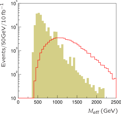
Figure 2: $M_{\rm eff}$ distribution for a typical mSUGRA point and SM backgrounds after cuts.

In Fig. 3(left) the 5$\sigma$ discovery reach in the plane of the mSUGRA parameters $m_{0}$ and $m_{1/2}$ is shown for integrated luminosities of 1,10,100,300 fb^-1 (red lines). The remaining parameters $A_{0}$ and $\tan\beta$ are fixed to 0 and 35, respectively, and sgn($\mu$) is chosen positive. The discovery reach depends only weakly on these parameters. Also shown are lines of constant squark and gluino masses. For (1,10,300) fb^-1 the mass reach for squarks and gluinos is approximately (1,2,2.5-3) TeV thus covering a very large part of the mSUGRA parameter space. The same applies qualitatively as well for a large part of the general MSSM with neutralino LSP.

Under the assumption of GUT unification of the gaugino mass parameters $M_{1},M_{2},M_{3}$ and sfermion mass parameters, the gluinos and squarks are heavier than the color-neutral superpartners due to renormalization group effects. Hence, the heavier charginos and neutralinos often appear in the decay chains of squarks. Their electro-weak decays often give rise to high-$p_{T}$ leptons whose efficient detectability provides an additional inclusive SUSY signature in many cases. In Fig. 3(right) the reach of the different lepton signatures (1 lepton, 2 like-sign (SS), 2 opposite-sign (OS), 3 leptons) plus $\not\!{E_{T}}$ is shown for 10 fb^-1.

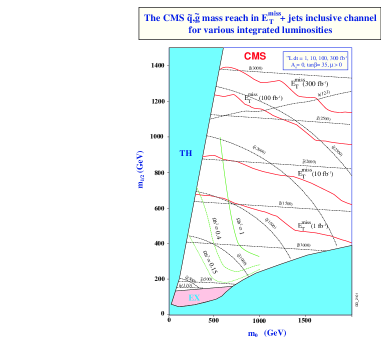
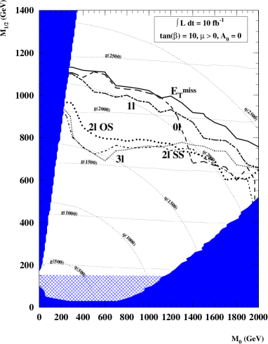
Figure 3: Left: LHC reach in the $m_{0}-m_{1/2}$ plane for inclusive discovery of SUSY in the missing transverse energy signature for the CMS experiment for an mSUGRA scenario with $\tan\beta=35$. Right: LHC reach for various inclusive SUSY signatures involving 0-3 leptons for 10 fb^-1.

II.4 Measurement of SUSY particle masses

While inclusive detection of SUSY processes is quite straight-forward at the LHC, the reconstruction of exclusive decay chains and the reconstruction of superpartner masses is quite involved due to various reasons: 1. the long decay chains of gluinos and squarks lead to signatures with many jets and leptons with huge combinatorics. 2. Due to the unknown longitudinal boost of the colliding partons of the initial state no kinematic constraints from the beam particles can be applied. 3. The event-by-event reconstruction of superpartner invariant masses is not possible due to the undetected LSP’s. The reconstruction of superpartner masses has therefore to rely on the detection of kinematic endpoints in the invariant masses of the detectable final state partons (jets and leptons) as well as on some knowledge about the involved decay chains.

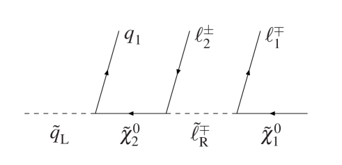
Figure 4: Typical decay cascade of a left-chiral squark

II.4.1 The $\tilde{q}_{L}\to q\ell^{+}\ell^{-}{\tilde{\chi}}^{0}_{1}$ decay chain

A frequently occurring and rather well reconstructible decay chain of a left-chiral squark via the second-lightest neutralino $\tilde{\chi}^{0}_{2}$ and a right-chiral slepton $\tilde{\ell}_{R}$ is shown in Fig. 4. The invariant mass distribution of the two opposite-sign same-flavor (OS-SF) leptons has a characteristic triangular shape which exhibits a distinct kinematic endpoint (’edge’) which involves the unknown masses of the three involved SUSY particles:

$$M_{\ell\ell}^{edge}=\sqrt{(M_{{\tilde{\chi}}_{2}^{0}}^{2}-M_{{\tilde{\ell}}}^{2})(M_{{\tilde{\ell}}}^{2}-M_{\tilde{\chi}_{1}^{0}}^{2})}/M_{\tilde{\ell}}\,.$$

In Fig. 5(left) the (OS-SF) di-lepton signal from $\chi^{0}_{2}$ decay is shown is shown together with the background from other SUSY decays and the (negligible) SM background. The SUSY background results mainly from wrongly combined and thus uncorrelated leptons from independent neutralino or chargino decays. It can be efficiently determined from the rate of OS-OF di-leptons in the data and then subtracted, as shown in the right part of Fig. 5. If the sleptons are heavier than ${\tilde{\chi}}_{2}^{0}$, the three-body decay ${\tilde{\chi}}^{0}_{2}\to\ell^{+}\ell^{-}{\tilde{\chi}}^{0}_{1}$ dominates which is different in shape and has an endpoint at the neutralino mass difference, $M_{{\tilde{\chi}}^{0}_{2}}-M_{{\tilde{\chi}}^{0}_{1}}$.

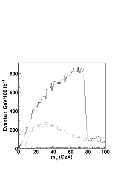
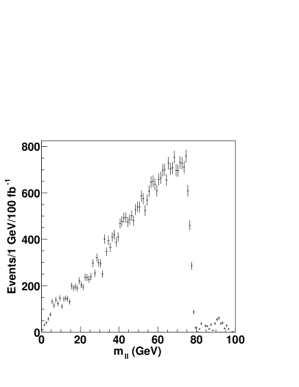
Figure 5: Left: opposite sign same flavor (OS-SF) di-lepton mass spectrum. The upper curve is from ${\tilde{\chi}}^{0}_{2}$ decays, the next curve is SUSY background, the lowest curve is SM background. Right: same after subtraction of the OS-OF rate which reduces the background from final states with uncorrelated lepton flavour.

While from the di-lepton endpoint alone no absolute superpartner masses can be extracted, further information can be obtained from the squark decay chain shown in Fig. 4 from various combinations of the leptons with a jet lester ; gjelsten . In particular, the following additional mass relations for kinematic edges can be exploited:

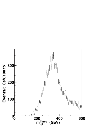
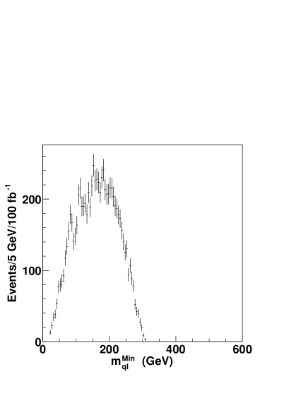
Figure 6: Various mass spectra which exhibit kinematic endpoints in squark decay cascades.

$$\bigl{(}m_{qll}^{2}\bigr{)}^{edge} = \frac{\bigl{(}m_{\tilde{q}_{L}}^{2}-m_{\tilde{\chi}_{2}^{0}}^{2}\bigr{)}\bigl{(}m_{\tilde{\chi}_{2}^{0}}^{2}-m_{\tilde{\chi}_{1}^{0}}^{2}\bigr{)}}{m_{\tilde{\chi}_{2}^{0}}^{2}}$$

$$\bigl{(}m_{ql}^{2}\bigr{)}^{edge}_{\rm min} = \frac{\bigl{(}m_{\tilde{q}_{L}}^{2}-m_{\tilde{\chi}_{2}^{0}}^{2}\bigr{)}\bigl{(}m_{\tilde{\chi}_{2}^{0}}^{2}-m_{\tilde{l}_{R}}^{2}\bigr{)}}{m_{\tilde{\chi}_{2}^{0}}^{2}}$$

$$\bigl{(}m_{ql}^{2}\bigr{)}^{edge}_{\rm max} = \frac{\bigl{(}m_{\tilde{q}_{L}}^{2}-m_{\tilde{\chi}_{2}^{0}}^{2}\bigr{)}\bigl{(}m_{\tilde{l}_{R}}^{2}-m_{\tilde{\chi}_{1}^{0}}^{2}\bigr{)}}{m_{\tilde{l}_{R}}^{2}}$$

$$\bigl{(}m_{qll}^{2}\bigr{)}^{\rm thres} = [(m_{\tilde{q}_{L}}^{2}+m_{\tilde{\chi}_{2}^{0}}^{2})(m_{\tilde{\chi}_{2}^{0}}^{2}-m_{\tilde{l}_{R}}^{2})(m_{\tilde{l}_{R}}^{2}-m_{\tilde{\chi}_{1}^{0}}^{2})$$

$$-(m_{\tilde{q}_{L}}^{2}-m_{\tilde{\chi}_{2}^{0}}^{2})\sqrt{(m_{\tilde{\chi}_{2}^{0}}^{2}+m_{\tilde{l}_{R}}^{2})^{2}(m_{\tilde{l}_{R}}^{2}+m_{\tilde{\chi}_{1}^{0}}^{2})^{2}-16m_{\tilde{\chi}_{2}^{0}}^{2}m_{\tilde{l}_{R}}^{4}m_{\tilde{\chi}_{1}^{0}}^{2}}$$

$$+2m_{\tilde{l}_{R}}^{2}(m_{\tilde{q}_{L}}^{2}-m_{\tilde{\chi}_{2}^{0}}^{2})(m_{\tilde{\chi}_{2}^{0}}^{2}-m_{\tilde{\chi}_{1}^{0}}^{2})]/(4m_{\tilde{l}_{R}}^{2}m_{\tilde{\chi}_{2}^{0}}^{2})$$

The labels “min” and “max” refer to the distribution constructed from the smaller and the larger of the two $q\ell$ masses. Furthermore “thres” refers to the threshold in the subset of the $m_{qll}$ distribution for which the angle between the two lepton momenta (in the slepton rest frame) exceeds $\pi/2$, which corresponds to $m_{ll}^{\rm edge}/\sqrt{2}<m_{ll}<m_{ll}^{\rm edge}$. The corresponding mass distributions are shown in Fig. 6. The position of the di-lepton edge can be measured to a statistical precision of better than 100 MeV and the edges involving jets can be measured to few GeV precision with 100 fb^-1 of data. In the case of the latter a systematic uncertainty from jet energy scale of approximately 1% has to be accounted for as well. Since the number of measurable edges in this scenario is larger than the number of involved superpartner masses, the absolute masses can be extracted from a simultaneous fit. The achievable precisions are listed in the first column of Table 2.

II.4.2 Gluino and third generation squarks

Knowing the masses of ${\tilde{\chi}}^{0}_{1},{\tilde{\chi}}^{0}_{2},{\tilde{\ell}}_{R}$, and ${\tilde{q}}_{L}$, gluinos can be reconstructed by adding another quark jet to the $q\ell\ell$ system. In particular when the decay proceeds through a $\tilde{b}$ squark, the tagging of two b-jets reduces combinatorial background. Knowing the mass of the LSP (from the joint fit to the kinematic edges described above), the momentum of the ${\tilde{\chi}}^{0}_{2}$ can be approximated by

$$\vec{p}({\tilde{\chi}}^{0}_{2})=\left(1-\frac{m({\tilde{\chi}_{1}^{0}})}{m(\ell\ell)}\right)\vec{p}_{\ell\ell}$$

if the ${\tilde{\chi}}^{0}_{1}$ carries negligible momentum in the ${\tilde{\chi}}^{0}_{2}$ rest frame, which in the SPS1a scenario is the case for events close to kinematic endpoint of the di-lepton mass spectrum. Knowing the ${\tilde{\chi}}^{0}_{2}$ momentum and mass, the sbottom mass can be subsequently reconstructed as the $b{\tilde{\chi}}^{0}_{2}$ invariant mass and the gluino mass as the $b\bar{b}{\tilde{\chi}}^{0}_{2}$ invariant mass. The reconstructed mass distributions in CMS for sbottom and gluino are shown for 300 fb^-1 are shown in Fig. 7 (left, middle). The mass difference between gluino and sbottom can be reconstructed without assumptions on the ${\tilde{\chi}}^{0}_{1}$ mass (Fig. 7, right) glusbot .

The reconstruction of $\tilde{t}$ squarks is more challenging. Initial studies are available stoplhc .

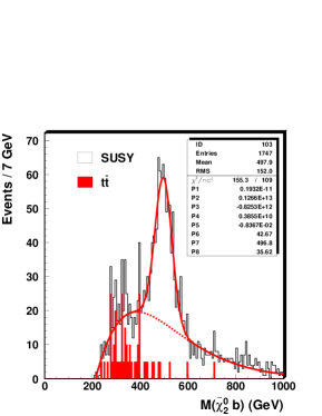
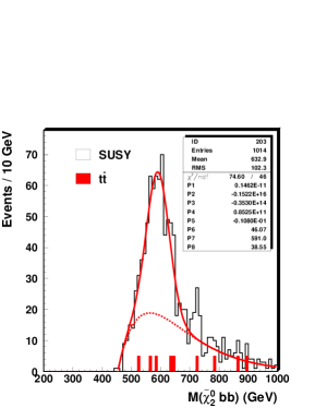
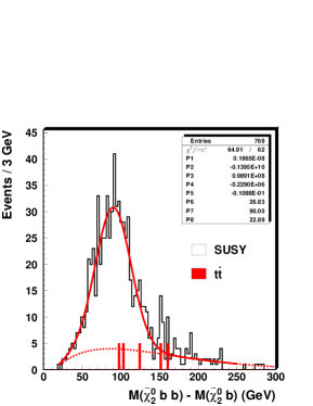
Figure 7: Reconstructed mass distribution for sbottom (left), gluino (middle), and for the gluino-sbottom mass difference (right) (from glusbot ).

II.4.3 Mass relation method

An alternative approach to mass reconstruction in the presence of long decay chains at the LHC, the mass relation method has recently been proposed massrelation . If one considers e.g. the decay chain $\tilde{g}\to\tilde{b}b_{2}\to{\tilde{\chi}}^{0}_{2}b_{1}b_{2}\to\tilde{\ell}b_{1}b_{2}\ell_{2}\to{\tilde{\chi}}^{0}_{1}b_{1}b_{2}\ell_{1}\ell_{2}$, the five superpartner mass $m_{{\tilde{\chi}}^{0}_{1}},m_{\tilde{\ell}},m_{{\tilde{\chi}}^{0}_{2}},m_{\tilde{b}},m_{\tilde{g}}$ can be calculated from the 5 4-momenta of the final state particles all of which except for $p_{{\tilde{\chi}}^{0}_{1}}$ are measured. Thus, the set of superpartner masses compatible with a single observed event corresponds to a 4-dimensional hypersurface in the 5-dimensional mass space. Since the exact location of the hypersurface is different for each event, the ensemble of hyper-surfaces from all events will have intersections at the true values of the five unknown masses. This method has been applied in a simplified version to the reconstruction of sbottom and gluino mass under the assumption that the other masses are known, in which case the hypersurface reduces to a line in ($m_{\tilde{g}},m_{\tilde{b}}$) space, i.e. for each pair of events a solution for ($m_{\tilde{g}},m_{\tilde{b}}$) is obtained up to a two-fold ambiguity. The advantages of the method are that it is based on exact kinematics without any approximation and that all events, not only the ones close to the kinematic endpoint, can be used. Furthermore, mass peaks are reconstructed rather than kinematic edges.

II.4.4 Sleptons

If sleptons are sufficiently light, they are produced at a decent rate in pp collisions through Drell-Yan pair production. For the SPS1a benchmark, the masses of the left- and righthanded selectrons and smuons are 143 GeV and 202 GeV, respectively. The total cross-section for smuon/selectron pair production is 91 fb. The signature are two opposite sign same flavor leptons, missing transverse energy and no jets. After subtraction of the opposite flavor background only a few events remain for 100 fb^-1. However, from a transverse mass estimator, the slepton mass can be estimated to a few GeV precision under favorable circumstances lytken .

Staus may frequently occur in the decays of ${\tilde{\chi}}^{0}_{2}$ if the $\tilde{\tau}_{1}$ is lighter than ${\tilde{\chi}}^{0}_{2}$, which is the case in SPS1a and in generally in mSUGRA models with significant $\tilde{\tau}$ mixing at large $\tan\beta$. Hadronic $\tau$ decays can be tagged typically at an efficiency of 50% for a QCD jet rejection factor of 100 at low luminosity. Selecting di-$\tau$ events with $\not\!{E_{T}}$ and large $M_{\rm eff}$ and again subtracting the same sign contribution, the invariant mass of the $\tau\tau$ decay products carries information about the $\tilde{\tau}$ mass in its endpoint. A mass estimate with a couple of GeV precision seems feasible but further study is needed.

II.4.5 Charginos

Recently a method has been proposed to observe the lighter chargino, ${\tilde{\chi}}^{\pm}_{1}$, frequently appearing in the decay chain of a left squark, $\tilde{q}_{L}\to{\tilde{\chi}}^{\pm}_{1}q$ via its decay ${\tilde{\chi}}^{\pm}\to W^{\pm}{\tilde{\chi}}^{0}_{1}\to q\bar{q}^{\prime}{\tilde{\chi}}^{0}_{1}$. The methods uses di-lepton events where the two leptons arise from the decay of the initial squark decaying into ${\tilde{\chi}}^{0}_{2}$ as described above. Assuming known masses for ${\tilde{\chi}}^{0}_{1},{\tilde{\chi}}^{0}_{2},\tilde{\ell}_{R},$ and $\tilde{q}_{L}$, the momentum of the ${\tilde{\chi}}^{0}_{1}$ from the ${\tilde{\chi}}^{0}_{2}$ can be reconstructed up to a two-fold ambiguity. After identification of hadronic $W$ bosons, the mass of the chargino can be reconstructed from the $W$ momentum, the reconstructed opposite-side ${\tilde{\chi}}^{0}_{1}$ and the total $\not\!{E_{T}}$ up to another two-fold ambiguity. After background subtraction of events in the side-bands of the reconstructed $W$ mass, a peak becomes visible in the reconstructed ${\tilde{\chi}}^{\pm}_{1}$ mass distribution. For a mSUGRA scenario with $m_{0}=100$ GeV, $m_{1/2}=300$ GeV, $A_{0}=-300$ GeV, $\tan\beta=6$, and sgn$(\mu)=+$, a 3$\sigma$ excess is achievable for 100 fb^-1 and a mass estimation with approximately 10% error seems feasible chargino .

II.4.6 Heavy gauginos

The left squarks predominantly decay via the gaugino-like neutralinos and charginos, i.e. usually ${\tilde{\chi}}^{0}_{2}$ and ${\tilde{\chi}}^{\pm}_{1}$ in mSUGRA models. While ${\tilde{\chi}}^{0}_{3}$ often is pure Higgsino, the heaviest neutralino ${\tilde{\chi}}^{0}_{4}$ and the heavy chargino ${\tilde{\chi}}^{\pm}_{2}$ have some gaugino admixture leading to a production of ${\tilde{\chi}}^{0}_{4}$ and ${\tilde{\chi}}^{\pm}_{2}$ in the $\tilde{q}_{L}$ decays with a branching ratio of a few percent. Four different decay chains via left and right sleptons (for the neutralino) and via a sneutrino (for the chargino) lead to di-lepton signatures of correlated flavor and charge with di-lepton masses significantly larger than for the ${\tilde{\chi}}^{0}_{2}$ decay described above. While it seems very hard to disentangle the four corresponding kinematic end-points, the observation of heavy gaugino production is possible with a dedicated analysis in a part of the mSUGRA parameter space, if $m_{0}$ is not too large. In particular, the highest mass end-point can be measured to a precision of approximately 4 GeV for the SPS1a scenario with 100 fb^-1 of data. Its unambiguous identification needs additional information, however heavygauginos .

II.5 Measurement of the ${\tilde{\chi}}^{0}_{2}$ Spin

The reconstruction of the superpartner spins is together with the determination of the their gauge quantum numbers the crucial test of SUSY. Spin information is carried by the scattering angle distribution of the primary pair of superpartners in their rest-frame. In hadron collisions, it is however hard to determine this frame due to the unknown longitudinal boost of the partonic initial state and due to the unobserved LSP’s in the final state. It is however possible to exploit angular distributions of the superpartner decay products in decay chains to obtain spin information. A particular example for a measurement of the ${\tilde{\chi}}^{0}_{2}$ spin has been worked out, again exploiting the $\tilde{q}_{L}\to q\ell^{+}\ell^{-}{\tilde{\chi}}^{0}_{1}$ cascade (see Fig. 4). Since the left squark always decays into a left-handed quark, the ${\tilde{\chi}}^{0}_{2}$ becomes polarized. Since in its decay the ${\tilde{\chi}}^{0}_{2}$ emits a scalar right slepton, the corresponding so-called near lepton will carry the polarization information of the ${\tilde{\chi}}^{0}_{2}$. Therefore one expects a charge asymmetry in invariant mass distribution of the quark and the near lepton, $m(\ell_{near}q)$. For $\ell^{+}q$ and $\ell^{-}\bar{q}$, the tree-level differential form the $m(\ell_{near}q)$ spectrum is $dP/dm\propto 4m^{3}$ while for $\ell^{-}q$ and $\ell^{+}\bar{q}$ it is $dP/dm\propto 4m(1-m^{2})$. These tree level distributions are not experimentally observable since anti-quarks cannot be distinguished from quarks and the near lepton cannot be distinguished from the far lepton. If the original (anti)-squarks are (at least partially) produced by the $qg\to\tilde{q}\tilde{g}$ and $\bar{q}g\to\tilde{\bar{q}}\tilde{g}$, the p.d.f. asymmetry due to the valence quarks in the protons can be exploited and more squarks than anti-squarks will be produced. The charge asymmetry from the far lepton is expected to be very small. Thus, forming both the invariant mass with the near and the far lepton dilutes the charge asymmetry but does not remove it. In Fig. 8(left) the reconstructed lepton-jet invariant mass distribution is shown for positive (squares) and negative (triangles) lepton charge. On the right, the resulting charge asymmetry is shown for 150 fb^-1 lhcspin .

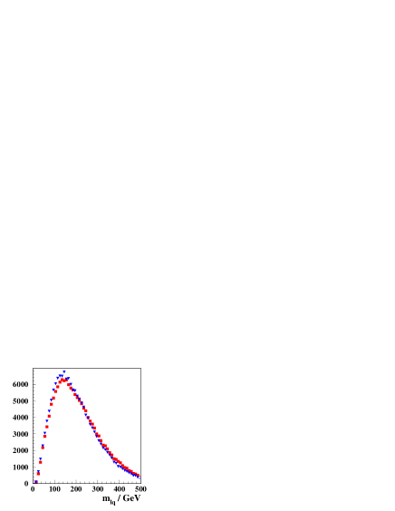
Figure 8: Left: Distribution of the charged lepton - jet invariant mass distribution for positive and negative leptons after detector simulation. Right: Observable charge asymmetry in the charged-lepton mass spectrum after detector simulation for 150 fb^-1 (from lhcspin ).

III SUSY AT THE LINEAR COLLIDER

III.1 Experimental environment

The International Linear Collider (ILC) is a projected electron positron collider at 500-1000 GeV center-of-mass energy with a luminosity of several $10^{34}{\rm cm}^{-2}{\rm s}^{-1}$ TESLA ; NLCreport ; acfareport . The energy will be tunable from the Z-pole up to the highest energy. Both beams can be polarized ($e^{-}$: 90%, $e^{+}$: 50-60%). The advantage of $e^{+}e^{-}$ collisions are the known, electro-weakly interacting initial state, the low level of instrumental and physics backgrounds and as a consequence the comparably low event rate which allows to record all collisions without any trigger requirements. Due to the high luminosity, unlike previous $e^{+}e^{-}$ machines, the ILC will have significant beam-beam interactions. These lead to a production of approximately 6$\times 10^{10}$ low-energetic photons per bunch-crossing at 500 GeV. About 10% of the events will have center-of-mass energies below 95% of the nominal energy. Therefore the beam-strahlung spectrum has to be monitored continously with data (e.g. acollinearity of Bhabha events) and corrected for. Backgrounds from collisions of beam-strahlung photons have been studied and were found to be small except for the very forward region for which dedicated highly-granular calorimeters have to be build.

III.2 Mass measurements

At the ILC the masses of the color-neutral superpartners can be measured in two different ways. First in continuum production, kinematic end-points and energy spectra can be used to extract simultaneously the involved masses. Second, the measurement of the shape of the production cross-section for various processes near threshold allows for a very precise extraction of the sum of the produced superpartner masses.

III.2.1 Sleptons

Sleptons are pair-produced in the reactions

$$e^{+}e^{-} \to \tilde{\ell}^{+}_{i}\tilde{\ell}^{-}_{j},\,\tilde{\nu}_{\ell}\,\bar{\tilde{\nu}_{\ell}}\hfill\qquad\qquad\qquad\ell=e,\,\mu,\,\tau\ {\rm\ and\ }\ [i,j=L,R\ {\rm\ or\ }\ 1,2]$$

via $s$-channel $\gamma/Z$ exchange and $t$-channel $\tilde{\chi}$ exchange for the first generation.

As an example, in Fig. 9(left) the measurable energy spectrum of the muons from the process $e^{+}_{L}e^{-}_{R}\to\tilde{\mu}_{R}^{+}\tilde{\mu}_{R}^{-}\to\mu^{+}{\tilde{\chi}}^{0}_{1}\mu^{-}\chi^{0}_{1}$ is shown sleptons . Events can be selected with negligible SM background. In particular background from W-pair production can be efficiently suppressed by choosing right-handed electrons in the initial state. SUSY backgrounds in this final state are generally small and can be suppressed in part by topological cuts. Due to the scalar nature of the smuons, the energy spectrum has a box shape. For the upper and lower end-points $E_{+/-}$, the slepton and LSP masses can be determined as

$$m_{\tilde{\ell}}=\frac{\sqrt{s}}{E_{-}+E_{+}}\,\sqrt{E_{-}\,E_{+}} m_{{\tilde{\chi}}^{0}_{1}}=m_{\tilde{\ell}}\,\sqrt{1-\frac{E_{-}+E_{+}}{\sqrt{s}/2}}.$$

The situation is more complicated in the case of $\tilde{\tau}$ sleptons due to the escaping neutrinos from $\tau$ decay leading to a depletion of the of the upper end-point and to elimination of the lower endpoint. However, if the mass of ${\tilde{\chi}}^{0}_{1}$ is known e.g. from smuon production, the shape and the upper end-point of the energy of the $\tau$ decay products can still be used to extract a precise mass value for $\tilde{\tau}_{1}$ as shown for the $\tau\to 3\pi\nu_{\tau}$ spectrum in Fig. 9(right).

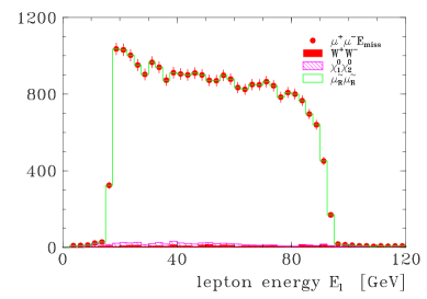
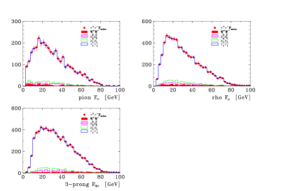
Figure 9: Left: Muon energy spectrum from the process $e^{+}_{L}e^{-}_{R}\to\tilde{\tau}_{1}\tilde{\tau}_{1}\to\mu^{+}\tilde{\chi}^{0}_{1}\mu^{-}\tilde{\chi}^{0}_{1}$ Right: Hadron energy spectrum of the decay $\tau\to 3\pi\nu_{\tau}$ from the process $e^{+}_{L}e^{-}_{R}\to\tilde{\tau}_{1}\tilde{\tau}_{1}$

Alternatively, the slepton masses can be extracted from a threshold scan as shown in Fig. 10 for right selectron production both in $e^{+}e^{-}$ and $e^{-}e^{-}$ collisions and for right smuon production. With measurements at five center-of-mass energies with only 10 fb^-1 per point a precision of $\cal O$(100 MeV) can be achieved. With this precision higher-order corrections and final width corrections have to be taken into account freitas .

Figure 10: cross-section for selectron and smuon pair production at threshold: $e^{+}_{L}e^{-}_{R}\to\tilde{e}_{R}\tilde{e}_{R}$ (left), $e^{-}_{L}e^{-}_{R}\to\tilde{e}_{R}\tilde{e}_{R}$ (middle), $e^{+}_{L}e^{-}_{R}\to\tilde{\mu}_{R}\tilde{\mu}_{R}$ (right). The error bars correspond to 10 fb^-1 per point.

III.2.2 Charginos and Neutralinos

Charginos and neutralinos are pair-produced

$$e^{+}e^{-} \to {\tilde{\chi}}^{\pm}_{i}{\tilde{\chi}}^{\mp}_{j}\qquad\qquad\qquad[i,j=1,2]$$ (1)

$$e^{+}e^{-} \to {\tilde{\chi}}^{0}_{i}{\tilde{\chi}}^{0}_{j}\qquad\qquad\qquad[i,j=1,\ldots,4]$$ (2)

via $s$-channel $\gamma/Z$ exchange and $t$-channel selectron or sneutrino exchange. The lightest chargino decays according to ${\tilde{\chi}}^{\pm}_{1}\to\ell^{\pm}\nu_{\ell}{\tilde{\chi}}^{0}_{1}$ either via an intermediate virtual or real $W^{\pm}$ boson or if kinematically possible via a real slepton. The second lightest neutralino decays according to ${\tilde{\chi}}^{0}_{2}\to\ell^{+}\ell^{-}{\tilde{\chi}}^{0}_{1}$ either via a virtual or real $Z$ boson or via a real slepton. In particular, if $m_{\tilde{\nu}}<m_{{\tilde{\chi}}^{0}_{2}}$, invisible $\tilde{\nu}$ decays may occur. For large mixing in the stau sector and for large values of $\tan\beta$ the $\tilde{\tau}_{1}$ slepton is often much lighter than the other sleptons which can lead to a significant enhancement of $\tau$ leptons in the chargino and neutralino final states. The production processes for $\tilde{\tau}$, $\chi^{0}_{2}$ and $\chi^{\pm}_{1}$ may therefore all lead to the same $\tau^{+}\tau^{-}+$ missing energy signature. Topological cuts and the use of polarized beams can help to disentangle the contributing SUSY processes. As in the case of sleptons, the chargino and neutralino masses can be measured from the lepton energy and mass spectra as well as from threshold scans. In the more difficult case of exclusive decays into $\tau$ final states, a mass precision of a few GeV can be achieved in the continuum and 0.5 GeV from a threshold scan. Significantly better precision can be achieved if electron and muon final states are produced with sufficient rate charneu .

III.2.3 Light Stop

Although squarks are often too heavy to be produced at a 1 TeV LC, the light scalar top quark may be lighter than the other squarks and therefore accessible in the reaction $e^{+}e^{-}\to\tilde{t}_{1}\tilde{t}_{1}\to b{\tilde{\chi}}^{+}_{1}\,\bar{b}{\tilde{\chi}}^{-}_{1}\to b\tau^{+}\nu{\tilde{\chi}}^{0}_{1}\,\bar{b}\tau^{-}\nu{\tilde{\chi}}^{0}_{1}$. The final state consists of two $b$-jets, two $\tau$’s and missing energy. The energy spectrum of the $b$-jets can be used to reconstruct the stop mass provided the neutralino and chargino masses are known feng . With a luminosity of 1000 fb^-1 the rate will be sufficient to achieve a mass resolution of 2 GeV. For a light scalar top quark, the decay chain $e^{+}e^{-}\to\tilde{t}_{1}\tilde{t}_{1}\to\to c{\tilde{\chi}}^{0}_{1}\,\bar{c}{\tilde{\chi}}^{0}_{1}$ has also been studied. From a measurement of the production cross-section with opposite beam polarizations, a measurement of both mass and mixing angle can be inferred finch .

III.2.4 Masses: Summary

The achievable superpartner mass precision of the ILC for the SPS1a scenario is summarized in Table 1 taken from lhclc .

Table 1: Sparticle masses and their expected precisions in Linear Collider experiments, SPS 1a mSUGRA scenario (from lhclc ).

	$m~{}[\mathrm{GeV}]$	$\Delta m~{}[\mathrm{GeV}]$	Comments
$\tilde{\chi}^{\pm}_{1}$	176.4	0.55	simulation threshold scan , 100 fb-1
$\tilde{\chi}^{\pm}_{2}$	378.2	3	estimate ${\tilde{\chi}}^{\pm}_{1}{\tilde{\chi}}^{\mp}_{2}$, spectra ${\tilde{\chi}}^{\pm}_{2}\to Z{\tilde{\chi}}^{\pm}_{1},\,W{\tilde{\chi}}^{0}_{1}$
$\tilde{\chi}^{0}_{1}$	96.1	0.05	combination of all methods
$\tilde{\chi}^{0}_{2}$	176.8	1.2	simulation threshold scan $\tilde{\chi}^{0}_{2}\tilde{\chi}^{0}_{2}$, 100 fb-1
$\tilde{\chi}^{0}_{3}$	358.8	3 – 5	spectra ${\tilde{\chi}}^{0}_{3}\to Z{\tilde{\chi}}^{0}_{1,2}$,  ${\tilde{\chi}}^{0}_{2}{\tilde{\chi}}^{0}_{3},{\tilde{\chi}}^{0}_{3}{\tilde{\chi}}^{0}_{4}$, 750 GeV, $>1000~{}\mathrm{fb}^{-1}$
$\tilde{\chi}^{0}_{4}$	377.8	3 – 5	spectra ${\tilde{\chi}}^{0}_{4}\to W{\tilde{\chi}}^{\pm}_{1}$,   ${\tilde{\chi}}^{0}_{2}{\tilde{\chi}}^{0}_{4},{\tilde{\chi}}^{0}_{3}{\tilde{\chi}}^{0}_{4}$, 750 GeV, $>1000~{}\mathrm{fb}^{-1}$
$\tilde{e}_{R}$	143.0	0.05	$e^{-}e^{-}$ threshold scan, 10 fb-1
$\tilde{e}_{L}$	202.1	0.2	$e^{-}e^{-}$ threshold scan 20 fb-1
$\tilde{\nu}_{e}$	186.0	1.2	simulation energy spectrum, 500 GeV, 500 fb-1
$\tilde{\mu}_{R}$	143.0	0.2	simulation energy spectrum, 400 GeV, 200 fb-1
$\tilde{\mu}_{L}$	202.1	0.5	estimate threshold scan, 100 fb-1 grannis
$\tilde{\tau}_{1}$	133.2	0.3	simulation energy spectra, 400 GeV, 200 fb-1
$\tilde{\tau}_{2}$	206.1	1.1	estimate threshold scan, 60 fb-1 grannis
$\tilde{t}_{1}$	379.1	2	estimate $b$-jet spectrum, $m_{\rm min}(\tilde{t})$, 1TeV, 1000 fb-1

III.3 Quantum numbers, couplings and mixings

Besides the precise measurement of the largest possible set of superpartner masses the measurement of quantum numbers, couplings, and mixings plays an important role in deciphering the supersymmetric model. In $e^{+}e^{-}$ collisions, due to the low background and the known initial state, various possibilities to extract quantum numbers and couplings exist. These range from the measurement of inclusive rates to the measurement of angular distributions in production and decay.

III.3.1 Spin determination

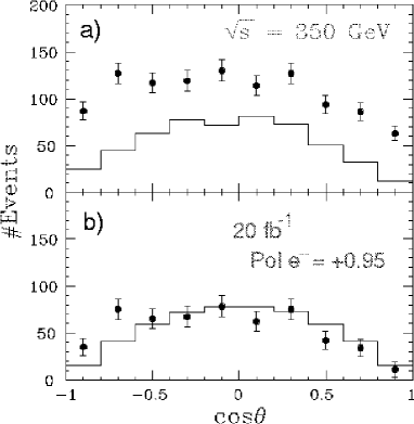
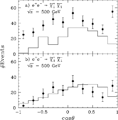
Figure 11: Distribution of the superpartner production angle for smuon (left) and charginos (right). The upper plots show both reconstructed solutions per event as points and the correct solution as full line; in the lower plots the combinatoric background is subtracted (from acfareport ).

The fundaments of SUSY rely on the superpartners’ spin differing by $\frac{1}{2}$ from their SM partners. It was shown in Sec. II.5 that at the LHC a unique spin determination is quite involved. At the LC, the spins of the superpartners can be determined directly from the production angle distributions. The scalar leptons exhibit a $\sin^{2}\theta$ distribution which can be reconstructed up to a twofold ambiguity in smuon pair-production. After subtraction of the combinatorial background the angular distribution is very clean (Fig. 11, left) acfareport . The situation is more complicated for charginos and neutralinos which exhibit a forward-backward asymmetry in the production angle due to their mixed U(1) and SU(2) couplings and the additional t-channel contribution. An example for chargino pair production is shown in Fig. 11, right). The forward-backward asymmetry and in particular the left-right polarization asymmetry provide sensitive observables in order to disentangle the chargino and neutralino mixing matrices gudiafb .

III.3.2 Chiral quantum numbers

In SUSY, the chiral (anti-)fermions are associated in an unambiguous way to scalars, i.e. $e^{-}_{L,R}\leftrightarrow\tilde{e}^{-}_{L,R}$ and $e^{+}_{L,R}\leftrightarrow\tilde{e}^{+}_{R,L}$. The four pair-production processes for left and right selectrons, $e^{+}e^{-}\to\tilde{e}^{+}_{R}\tilde{e}^{-}_{R}$, $e^{+}e^{-}\to\tilde{e}^{+}_{L}\tilde{e}^{-}_{L}$, $e^{+}e^{-}\to\tilde{e}^{+}_{R}\tilde{e}^{-}_{L}$, $e^{+}e^{-}\to\tilde{e}^{+}_{L}\tilde{e}^{-}_{R}$ can be disentangled from their different dependence of the cross-section to polarized electron and positron beams. From Fig. 12, it can be seen that e.g. $e^{+}e^{-}\to\tilde{e}^{+}_{R}\tilde{e}^{-}_{R}$ and $e^{+}e^{-}\to\tilde{e}^{+}_{L}\tilde{e}^{-}_{R}$ have practically identical behavior of the cross-section as a function of the electron polarization but differ completely as a function of the positron polarization gudipol . The t-channel contribution to the production cross-sections is sensitive to the SUSY Yukawa coupling $\hat{g}(e\tilde{e}{\tilde{\chi}}^{0})$ which is fundamentally related to the SM gauge couplings. The SU(2) and U(1) SUSY Yukawa couplings can be determined to a precision of 0.7% and 0.2%, respectively with 500 fb^-1 at 500 GeV in a SPS1a scenario sleptons .

Figure 12: Separation of the selectron pair $\tilde{e}_{L}^{-}\tilde{e}^{+}_{R}$ in $e^{+}e^{-}\to\tilde{e}^{+}_{L,R}\tilde{e}^{-}_{L,R}$ may not be possible with electron polarization only (left); if, however, both beams are polarized, the $RR$ configuration separates the pairs and the association of the selectrons to the chiral quantum numbers can be experimentally tested (from gudipol ).

III.3.3 Stau mixing angle

In the third generation large mixing effects are expected. Again, beam polarization is vital to measure the stau mixing angle from measuring the cross-section for $e^{+}e^{-}\to\tilde{\tau}_{1}\tilde{\tau}_{1}$ with polarized beams. This allows for a measurement of $\cos{2\theta_{\tilde{\tau}}}=-0.84\pm 0.04$ in an SPS1a scenario for 500 fb^-1 staumix . Further, independent information can be obtained from the measurement of the $\tau$ lepton polarization in $\tilde{\tau}_{1}\to\tau{\tilde{\chi}}^{0}_{1}\to\pi^{\pm}\nu_{\tau}{\tilde{\chi}}^{0}_{1}$. For known $\tilde{\tau}$ mixing angle, this information can be used to gain sensitivity to $\tan\beta$.

III.3.4 CP-violation in SUSY decays

Many studies of SUSY at LHC and LC have focused on a (often constrained) MSSM with real parameters. The general MSSM Lagrangian however allows for CP-violating complex parameters. As an example, the U(1) gaugino mass parameter $M_{1}$ and the Higgsino mixing parameter $\mu$ may have complex phases $\phi_{M_{1}},\phi_{\mu}$. These phases may be accessed in angular correlations of the decay products in neutralino decay bartl . An experimental study of how well these correlations can be measured is still lacking.

Similarly, CP-violating phases of the tri-linear couplings $A_{\tau},A_{b},A_{t}$ may be accessed in studying the branching fractions of the third generation sfermions an analyze them together with their masses and production cross sections in a global fit hesselbach .

III.4 Constraining Dark Matter

The SUSY LSP provides an excellent candidate for dark matter. Recent measurements of temperature fluctuations of the cosmic microwave background by the WMAP satellite wmap strongly constrain the SUSY LSP properties and therefore point to certain regions in the MSSM parameter space. Of particular interest for experimental studies at colliders is the co-annihilation region in which the neutralino annihilation is enhanced by the t-channel process ${\tilde{\chi}}\tilde{\tau}\to\tau\gamma$ which contributes significantly only if the mass difference $\Delta m=m(\tilde{\tau})-m({\tilde{\chi}}^{0}_{1})$ is small. The relic dark matter density depends critically on this mass difference. With the next generation of CMB experiments, in particular Planck, the DM density can be measured at the 2-3% level. It is therefore imperative to match this precision at colliders.

If $\Delta m$ is small (typically below 10 GeV), the staus decay with small visible energy and the signature is only a few soft charged tracks accompanied by large missing energy. Two-photon background is becoming severe unless it can be efficiently vetoed by the detection of very forward scattered electrons. In the very forward region significant energy induced by beam-beam-interactions is deposited. This energy deposition in the most forward calorimeter, is shown in Fig. 13 for two interaction region designs without (left) and with (right) a crossing-angle of the two incoming beams. The detection of energetic electrons is possible down to angles of 3.5 (5.7) mrad without (with) crossing angle if the calorimeter is finely segmented.

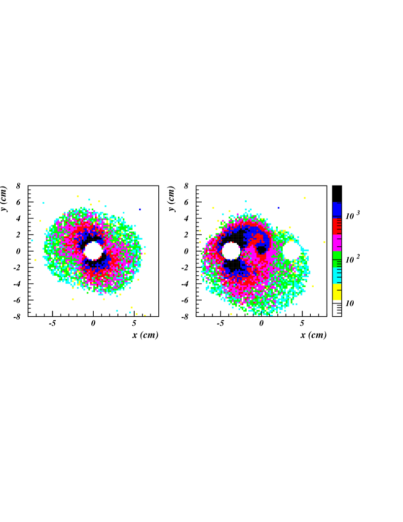
Figure 13: Energy deposition from beam-strahlung (in GeV) in the forward detector region (3.7m from the interaction point) without (left) and with (right) a 10 mrad half-angle crossing angle.

The pair production of staus in the small-$\Delta m$ region has been studied in martyn-smalldm and bambade for various MSSM parameter sets. With appropriate cuts, detection and a precise measurement of the $\tilde{\tau}$ mass is possible down to $\Delta m$ $\sim$3 GeV. The resulting precision on the prediction for the dark matter density ranges from 2 to 6%, depending on the $\tilde{\tau}$ mass and on $\Delta m$. This precision matches the anticipated precision of the Planck satellite of 2%. As an example the hadronic energy spectra for $\tau$ decays from the process $e^{+}_{L}e^{-}_{R}\to{\tilde{\tau}}_{1}\,{\tilde{\tau}}_{1}\to\tau^{+}{\tilde{\chi}}^{0}_{1}\,\,\tau^{-}{\tilde{\chi}}^{0}_{1}$ as shown after detector simulation and cuts together with the two-photon background for $\Delta m=5$ GeV (Model Point D^′ from battagliabench ).

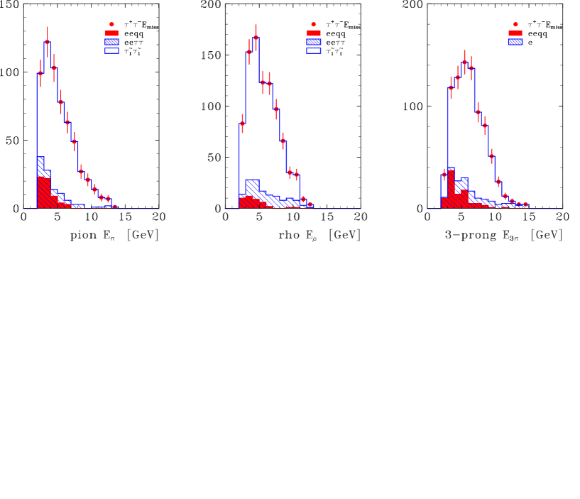
Figure 14: Hadron energy spectra $E_{\pi}$ of $\tau\to\pi\nu_{\tau}$, $E_{\rho}$ of $\tau\to\rho\nu_{\tau}$ and $E_{3\pi}$ of $\tau\to 3\pi\nu_{\tau}$ decays from the reaction $e^{+}_{L}e^{-}_{R}\to{\tilde{\tau}}_{1}\,{\tilde{\tau}}_{1}\to\tau^{+}{\tilde{\chi}}^{0}_{1}\,\,\tau^{-}{\tilde{\chi}}^{0}_{1}$ and two-photon production assuming head-on collision. Model D’, $m_{{\tilde{\tau}}_{1}}=217.5\;\mathrm{GeV},\ \Delta m=5.1\;\mathrm{GeV}$, $\sqrt{s}=600\;\mathrm{GeV}$ and ${\cal L}=300\;\mathrm{fb}^{-1}$

IV LHC/LC INTERPLAY

The ultimate goal of measurements of the properties of superpartners at LHC and LC will be the extraction of the complete set of parameters of the low energy MSSM Lagrangian. The previous sections have already indicated the complementarity of the possibilities at the LHC (large mass reach for squarks and gluinos) and the LC (precision measurements of color-neutral part of spectrum). In this section, we will discuss the additional benefit of simultaneous interpretation and possibly simultaneous data analysis if both machines run concurrently. This aspect has recently been studied in the international LHC/LC working group lhclc . Without aiming for completeness, a few examples of this interplay will be given in the following.

IV.1 Joint analysis of superpartner masses

It has been shown in Section II that mass reconstruction of squarks and gluinos at the LHC suffers from the unknown masses of the lighter states, in particular the LSP and the sleptons. Under favourable circumstances, they can be reconstructed from a joint fit of various kinematic endpoints to moderate accuracy. However a strong correlation of e.g. the squark mass and the LSP neutralino mass remains (see Fig. 15). A precise measurement of slepton, chargino, and neutralino masses at the LC removes these correlations and improves the precision of squark and gluino masses considerably even in a situation where the latter are not directly accessible at the LC. The expected precisions on some of the masses in a SPS1a scenario are shown Tab. 2. It should be noted that the precision on squark and gluino masses in the combined analysis is dominated by uncertainties on the hadronic energy scale of the LHC experiments, assumed to be 1%.

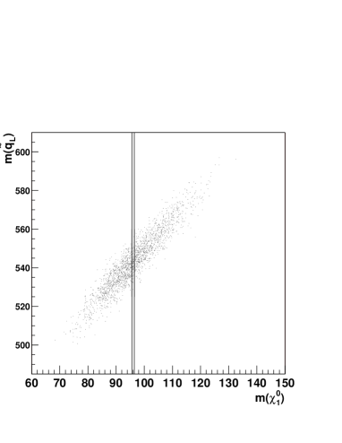
Figure 15: Correlation between left squark (left) and lighter sbottom (right) and the LSP mass at the LHC.

Table 2: The RMS values of the mass distribution in the case of the LHC alone, and together with the ILC measurement of $m_{\tilde{\chi}_{1}^{0}}$. Only the masses resulting from the edge analyses are given. All numbers in GeV.

	LHC	LHC+ILC
$\Delta m_{\tilde{\chi}_{1}^{0}}$	4.8	0.19
$\Delta m_{\tilde{l}_{R}}$	4.8	0.34
$\Delta m_{\tilde{\chi}_{2}^{0}}$	4.7	0.24
$\Delta m_{\tilde{q}_{L}}$	8.7	4.9
$\Delta m_{\tilde{b}_{1}}$	13.2	10.5

IV.2 ILC mass predictions for LHC searches

At the ILC, the SUSY parameters which govern the chargino-neutralino sector, i.e. the U(1) and SU(2) gaugino mass parameters $M_{1},M_{2}$, the Higgsino mixing parameter $\mu$ and $\tan\beta$ can be uniquely and precisely extracted from the measurements of masses and polarized cross-sections of the lightest gauginos, ${\tilde{\chi}}^{0}_{1},{\tilde{\chi}}^{0}_{2},$ and ${\tilde{\chi}}^{\pm}_{1}$. These parameters can in turn be used to predict the masses of the heavier members ${\tilde{\chi}}^{0}_{3},{\tilde{\chi}}^{0}_{4}$ and ${\tilde{\chi}}^{\pm}_{2}$ within the framework of the general MSSM. With such a mass prediction, the search for the (often small) signals of the heavy gauginos can be substantially facilitated. The search for an edge in the di-lepton mass spectrum becomes transformed into a single hypothesis test, thus inceasing the statistical power of the LHC data for this specific hypothesis.

Should in turn the predicted state be observed at the LHC, its measured mass can be fed back into the SUSY parameter analysis and considerably improve the achieavble precision.

Furthermore, the comparison of the predicted ${\tilde{\chi}}^{0}_{4}$ mass from LC measurements and the measured mass at the LHC allows to test for models beyond the MSSM. This has recently been shown gudinmssm for a NMSSM, where in contrast to the MSSM five neutralinos are predicted with a mass spectrum not satisfying the MSSM relations.

IV.3 Global MSSM fits and reconstruction of the theory

Ultimately, the goal is to measure the complete set of electro-weak scale parameters of the SUSY Lagrangian. At tree level, the parameter determination can proceed sector by sector, e.g. the chargino sector is completely determined by the three parameters $M_{2},\mu,\tan\beta$. However, with the anticipated precision of ILC measurements, higher order corrections to masses, cross-sections, and branching ratios are not negligible. At loop-level in principle every observable depends on the full set of SUSY parameters. An analytic procedure to extract the Lagrangian parameters from data is no longer possible. Instead, a global fit of the Lagrangian parameters to the complete set of SUSY observabales at LHC and LC will be necessary.

Two programs, SFITTER sfitter and Fittino fittino have been developed to achieve this goal. As an example, a recent result from Fittino is explained here. A MSSM with 19 free parameters has been chosen as the theoretical basis. It is derived from the full MSSM but assuming real couplings, flavour diagonal sfermion mass matrices and universality of the soft SUSY breaking parameters of the first two generations. For the theoretical predictions for the observables as a function of the parameters the SPHENO spheno program has been used. This code includes higher-order corrections whereever they have been calculated. The program is interfaced via the ’SUSY Les Houches Accord’ (SLHA) slha , a convention to exchange SUSY parameter information between various programs in a coherent way. Therefore it is possible to replace the actual SUSY code behind Fittino in order to perform comparisons. As simulated measurements, the masses measureable at LHC and LC as explained in the previous sections have been used. In addition polarized cross-section measurements at 500 and 1000 GeV LC have been input with accuracies based on estimates from the expected statistical errors, but including systematic errors of 1% in each case. For the true values of the parameters, the SPS1a scenario has been chosen but nowhere in the fit any assumptions on the particular SUSY breaking mechanism have been made. Special care was given to a fitting strategy which does not make use of any a-priori knowledge of the parameters. In particular, suitable start values for the parameters have been estimated from the measurements using tree-level relations between various observable and parameters sector by sector. In order to yield a correctly converging fit an iterative procedure has to be applied which does not leave free all parameters from the beginning. Only after this preparatory phase the full fit can be performed with all parameters left free. The example result for SPS1a is shown in Table 3. The importance of higher-order corrections can be seen from comparing the tree-level parameter estimates with their final values. It has been verified that the obtained fit errors are consistent with the fluctation of the fitted parameters in many repeated measurements. It should be noted that neither LHC nor LC input alone can constrain the assumed model enough to yield a converging fit. It was also shown, that due to the mutual influence of many parameters in determining a single observable, wrong assumptions of un-fitted parameters lead to wrong central values for the fit parameters. The lesson from this excercise are: first, it is possible, at least for a favourable scenario like SPS1a, to extract the complete electro-weak scale Lagrangian from the future measurements of LHC and LC without strong assumptions on the particular SUSY breaking scenario. Second, the fact that results from both LHC and LC are necessary to obtain this result nicely shows the strong interplay between both machines. Third, the achievable experimental precision clearly requires the knowledge of theoretical predictions beyond leading order. The definition of a clear scheme to extract well-defined parameters at higher orders is currently being worked out in the Supersymmetry Parameter Analysis (SPA) project spa .

The extracted parameters of the electro-weak scale MSSM Lagrangian can then be extrapolated to high (GUT, Planck) scales (Fig. 16 in order to determine distinct patterns of unification and reconstruct the underlying fundamental theory of SUSY breaking porod .

Table 3: The Fittino SPS1a fit result. The left column shows the assumed SPS1a values, the middle column represents the result of the intermediate fit without $m_{\mathrm{top}}$, and the right column shows the result of the final fit. All SPS1a input values of the parameters are reconstructed.

Parameter	SPS1a value	Tree-level	Final fit result
		estimate
$\tan\beta$	10.0	9.97	$10.0\pm 0.3$
$\mu$	358.64 GeV	354.4 GeV	$358.6\pm 1.1$ GeV
$X_{\tau}$	-3837.23 GeV	-3533.0 GeV	$-3837.2\pm 131.0$ GeV
$M_{\tilde{e}_{R}}$	135.76 GeV	150.2 GeV	$135.76\pm 0.39$ GeV
$M_{\tilde{\tau}_{R}}$	133.33 GeV	141.0 GeV	$133.33\pm 0.75$ GeV
$M_{\tilde{e}_{L}}$	195.21 GeV	202.7 GeV	$195.21\pm 0.18$ GeV
$M_{\tilde{\tau}_{L}}$	194.39 GeV	206.6 GeV	$194.4\pm 1.18$ GeV
$X_{\mathrm{top}}$	-506.388 GeV	-43.5 GeV	$-506.4\pm 29.5$ GeV
$X_{\mathrm{bottom}}$	-4441.0 GeV	-3533.0 GeV	$-4441.1\pm 1765$ GeV
$M_{\tilde{d}_{R}}$	528.14 GeV	567.3 GeV	$528.2\pm 17.6$ GeV
$M_{\tilde{b}_{R}}$	524.718 GeV	566.0 GeV	$524.7\pm 7.7$ GeV
$M_{\tilde{u}_{R}}$	530.253 GeV	566.9 GeV	$530.2\pm 19.1$ GeV
$M_{\tilde{t}_{R}}$	424.382 GeV	373.7 GeV	$424.4\pm 8.54$ GeV
$M_{\tilde{u}_{L}}$	548.705 GeV	581.3 GeV	$548.7\pm 5.2$ GeV
$M_{\tilde{t}_{L}}$	499.972 GeV	575.4 GeV	$500.0\pm 8.1$ GeV
$M_{1}$	101.809 GeV	99.07 GeV	$101.81\pm 0.06$ GeV
$M_{2}$	191.7556 GeV	195.08 GeV	$191.76\pm 0.10$ GeV
$M_{3}$	588.797 GeV	630.5 GeV	$588.8\pm 7.9$ GeV
$m_{A}$	399.767 GeV	399.8 GeV	$399.8\pm 0.71$ GeV
$m_{\mathrm{top}}$	174.3 GeV	174.3 GeV	$174.3\pm 0.34$ GeV

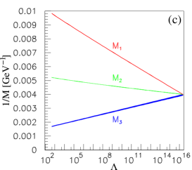
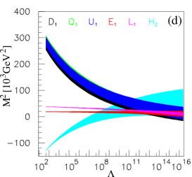
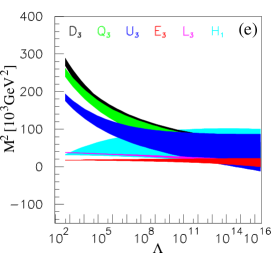
Figure 16: Renormalization group evolution of the MSSM parameters determined from LHC and LC measurements to the GUT scale.