Non-Linear Effects in High Energy Hadronic Interactions

Abstract

The influence of non-linear interaction effects on the characteristics of hadronic collisions and on the development of extensive air showers (EAS) is investigated. Hadronic interactions are treated phenomenologically in the framework of Gribov’s Reggeon approach with non-linear corrections being described by enhanced (Pomeron-Pomeron interaction) diagrams. A re-summation algorithm for higher order enhanced graphs is proposed. The approach is applied to develop a new hadronic interaction model QGSJET-II, treating non-linear effects explicitely in individual hadronic and nuclear collisions. The model is applied to EAS modelization and the obtained results are compared to the original QGSJET predictions. Possible consequences for EAS data interpretation are discussed.

1 Introduction

Currently the physics of hadronic interactions remains one of the most intriguing fields both for experimental and for theoretical research. Being the subject of investigations in collider experiments, it has a different role in high energy cosmic ray (CR) studies. There, a proper understanding of hadronic interaction mechanisms is of vital importance for a correct interpretation of CR data, for a reconstruction of energy spectra and of particle composition of the primary cosmic radiation, and finally, for inferring informations on the sources of CR particles, whose energies extend to ZeV region, exceeding by far those attainable at man-made machines.

Despite a significant progress in QCD over the past two decades, only phenomenological treatment is generally possible for minimum-bias hadron-hadron (hadron-nucleus, nucleus-nucleus) collisions. In particular, Gribov’s Reggeon scheme[1] proved to be a suitable framework for developing successful model approaches, like Quark-Gluon String or Dual Parton models,[2] which in turn provided a basis for a number of Monte Carlo (MC) generators of hadronic and nuclear collisions, extensively used in accelerator or CR fields, e.g., DPMJET,[3] VENUS,[4] or QGSJET.[5, 6]

Still, all the mentioned MC models are based on a linear picture, the elastic scattering amplitude being defined by (quasi-)eikonal contributions of independent Pomeron exchanges. Meanwhile, in the limit of very high energies one expects a significant increase of parton density in colliding hadrons (nuclei), which gives rise to essential non-linear interaction effects.[7] On the other hand, in Gribov’s scheme the latter are traditionally described as Pomeron-Pomeron interactions.[8, 9] Here we propose a re-summation procedure both for enhanced contributions to the elastic scattering amplitude and for various unitarity cuts of the corresponding diagrams. This gives us a possibility to account for non-linear corrections when calculating hadron-hadron cross sections and to develop a new MC model, QGSJET-II,[10] which treats non-linear effects explicitely in individual hadronic and nuclear collisions. The model is applied to simulate extensive air showers (EAS), induced by CR particles in the atmosphere, which allows to investigate the influence of non-linear corrections on the air shower characteristics and to draw possible consequences for EAS data interpretation.

2 Linear Scheme

Gribov’s Reggeon approach[1] describes a high energy hadron-hadron collision as a multiple scattering process, where elementary re-scatterings are treated phenomenologically as Pomeron exchanges – Fig. 1.

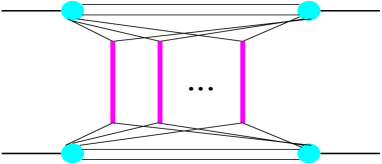
Figure 1: A general multi-Pomeron contribution to hadron-hadron scattering amplitude. Elementary scattering processes (vertical thick lines) are described as Pomeron exchanges; thin lines correspond to constituent partons, to which Pomerons are coupled.

Thus, hadron $a$ – hadron $d$ elastic amplitude can be obtained summing over multi-Pomeron exchange contributions[2, 11] (see also Ref. dre01):

$$f_{ad}(s,b) = i\sum_{j,k}C_{j}^{a}\,C_{k}^{d}\,\sum_{n=1}^{\infty}\frac{1}{n!}\int\!\left[\prod_{l=1}^{n}dx_{l}^{+}dx_{l}^{-}\,\lambda_{j}^{a}\,\lambda_{k}^{d}\,G_{ad}^{\mathbb{P}}(x_{l}^{+}x_{l}^{-}s,b)\right]$$ (1)

$$\times N_{a}^{(n)}(x_{1}^{+},...,x_{n}^{+})\;N_{d}^{(n)}(x_{1}^{-},...,x_{n}^{-}),$$

where $s$ and $b$ are the c.m. energy squared and the impact parameter of the interaction, $G_{ad}^{\mathbb{P}}(x^{+}x^{-}s,b)$ is the unintegrated Pomeron exchange eikonal (for fixed values of Pomeron light cone momentum shares $x^{\pm}$), and $N_{a}^{(n)}(x_{1},...,x_{n})$ is the light cone momentum distribution of constituent partons – “Pomeron ends” (here, quark-antiquark pairs). $C_{j}^{a}$, $\lambda_{j}^{a}$ are the relative weights and strengths of diffractive eigenstates of hadron $a$ in the Good-Walker formalism;[13] $\sum_{j}C_{j}^{a}=1$, $\sum_{j}C_{j}^{a}\,\lambda_{j}^{a}=1$. In particular, a two-component model ($j=1,2$) with one passive component, $\lambda_{2}^{a}\equiv 0$, corresponds to the quasi-eikonal approach, where $\lambda_{1}^{a}\equiv 1/C_{1}^{a}$ is the shower enhancement coefficient.[2]

Eq. (1) can be greatly simplified assuming that the integral over light cone momenta can be factorized:

$$\int\left[\prod_{l=1}^{n}dx_{l}^{+}dx_{l}^{-}\;G_{ad}^{\mathbb{P}}(x_{l}^{+}x_{l}^{-}s,b)\right]\,N_{a}^{(n)}(x_{1}^{+},...,x_{n}^{+})\;N_{d}^{(n)}(x_{1}^{-},...,x_{n}^{-})$$

$$=\left[\int dx^{+}dx^{-}\,G_{ad}^{\mathbb{P}}(x^{+}x^{-}s,b)\,N_{a}^{(1)}(x^{+})\;N_{d}^{(1)}(x^{-})\right]^{n}$$ (2)

This leads to traditional eikonal formulas:

$$f_{ad}(s,b) = i\sum_{j,k}C_{j}^{a}\,C_{k}^{d}\,\left[1-e^{-\lambda_{j}^{a}\,\lambda_{k}^{d}\,\chi_{ad}^{\mathbb{P}}(s,b)}\right]$$ (3)

$$\chi_{ad}^{\mathbb{P}}(s,b) \equiv \int dx^{+}dx^{-}\,G_{ad}^{\mathbb{P}}(x^{+}x^{-}s,b)\;N_{a}^{(1)}(x^{+})\;N_{d}^{(1)}(x^{-})$$ (4)

In this scheme the Pomeron is an effective description of a microscopic parton cascade which mediates the interaction between the projectile and the target hadrons. It is convenient to divide the latter into two parts:“soft” cascade of partons of small virtualities $|q^{2}|<Q_{0}^{2}$, and a perturbative parton evolution at $|q^{2}|>Q_{0}^{2}$, where $Q_{0}^{2}$ is some cutoff for pQCD being applicable. Correspondingly, a “general Pomeron” will consist of two contributions: “soft” Pomeron for a pure non-perturbative process (all $|q^{2}|<Q_{0}^{2}$) and a “semi-hard Pomeron” for a cascade which at least partly develops in the high virtuality region (some $|q^{2}|>Q_{0}^{2}$)[6, 12, 15] – Fig. 2:

$$G_{ad}^{\mathbb{P}}(\hat{s},b)=G_{ad}^{{\mathbb{P}}_{\rm soft}}(\hat{s},b)+G_{ad}^{{\mathbb{P}}_{\rm sh}}(\hat{s},b)$$ (5)

The advantage of such a procedure is that in very high energy limit the “general Pomeron” is dominated by its semi-hard component and the energy dependence of the eikonal $G_{ad}^{\mathbb{P}}(\hat{s},b)$ is governed asymptotically by the perturbative QCD evolution.

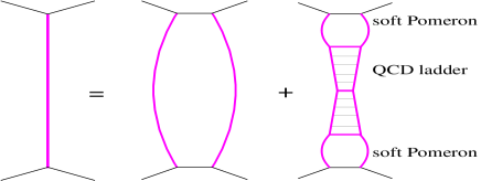
Figure 2: A “general Pomeron” (l.h.s.) consists of the “soft” and the “semi-hard” Pomerons – correspondingly the 1st and the 2nd contributions on the r.h.s.

The soft Pomeron eikonal can chosen in the usual form:[2]

$$G_{ad}^{{\mathbb{P}}_{\rm soft}}(\hat{s},b)=\frac{\gamma_{a}\,\gamma_{d}\,(\hat{s}/s_{0})^{\alpha_{{\mathbb{P}}}(0)-1}}{R_{a}^{2}+R_{d}^{2}+\alpha_{{\mathbb{P}}}^{\prime}(0)\,\ln\!\frac{\hat{s}}{s_{0}}}e^{-\frac{b^{2}}{4\left(R_{a}^{2}+R_{d}^{2}+\alpha_{{\mathbb{P}}}^{\prime}(0)\,\ln\!\frac{\hat{s}}{s_{0}}\right)}},$$ (6)

where $s_{0}\simeq 1$ GeV² is the hadronic mass scale, $\alpha_{{\mathbb{P}}}(0)$ and $\alpha_{{\mathbb{P}}}^{\prime}(0)$ are the intercept and the slope of the Pomeron Regge trajectory, and $\gamma_{a}$, $R_{a}^{2}$ are the coupling and the slope of Pomeron-hadron $a$ interaction vertex.

The dominant contribution to the semi-hard Pomeron comes from hard scattering of gluons and sea quarks and can be represented by a piece of QCD ladder sandwiched between two soft Pomerons – Fig. 2; the corresponding eikonal may be written as[6, 12, 15]

$$G_{ad}^{{\mathbb{P}}_{\rm sh}}(\hat{s},b) = \frac{1}{2}\sum_{I,J=g,\bar{q}}\int\!d^{2}b^{\prime}\int\!\frac{dx_{h}^{+}}{x_{h}^{+}}\frac{dx_{h}^{-}}{dx_{h}^{-}}\;\sigma_{IJ}^{\rm QCD}(x_{h}^{+}x_{h}^{-}\hat{s},Q_{0}^{2})$$ (7)

$$\times G_{aI}^{{\mathbb{P}}_{\rm soft}}(s_{0}/x_{h}^{+},b^{\prime})\;G_{dJ}^{{\mathbb{P}}_{\rm soft}}(s_{0}/x_{h}^{-},|\vec{b}-\vec{b}^{\prime}|)$$

Here $\sigma_{IJ}^{\rm QCD}(x_{h}^{+}x_{h}^{-}\hat{s},Q_{0}^{2})$ is the contribution of the parton ladder with the virtuality cutoff $|q^{2}|>Q_{0}^{2}$; $I,J$ and $x_{h}^{+},x_{h}^{-}$ are the types and the relative light cone momentum shares of the ladder leg partons. The eikonal $G_{aI}^{{\mathbb{P}}_{\rm soft}}(\hat{s},b^{\prime})$, describing parton $I$ momentum and impact parameter distribution in the soft Pomeron at virtuality scale $Q_{0}^{2}$, is defined by Eq. (6), neglecting the small slope of Pomeron-parton coupling $R_{I}^{2}\sim 1/Q_{0}^{2}\sim 0$ and using a parameterized Pomeron-parton $I$ vertex $\gamma_{I}(x_{h})$, $x_{h}=s_{0}/\hat{s}$. Usual hadronic parton momentum distribution functions (PDFs) can be obtained convoluting $G_{aI}^{{\mathbb{P}}_{\rm soft}}$ with the constituent parton distribution $N_{a}^{(1)}$ and integrating over the parton impact parameter $b^{\prime}$:

$$x\,f_{I/a}(x,Q_{0}^{2})=\int\!d^{2}b^{\prime}\int_{x}^{1}\!dx^{+}\;N_{a}^{(1)}(x^{+})\;G_{aI}^{{\mathbb{P}}_{\rm soft}}(s_{0}\,x^{+}/x,b^{\prime})$$ (8)

Thus, the contribution of semi-hard processes to the integrated eikonal (4), integrated over the impact parameter $b$, can be written[12, 15] as a convolution of hadronic PDFs $f_{I/a(J/d)}(x,Q^{2})$ (obtained by evolving the input PDFs (8) from $Q_{0}^{2}$ to $Q^{2}$) with the parton scatter cross section $d\sigma_{ij}^{2\rightarrow 2}/dp_{t}^{2}$:

$$\int\!d^{2}b\,\chi_{ad}^{{\mathbb{P}}_{\rm sh}}(s,b) = \frac{1}{2}\int\!dx_{h}^{+}\,dx_{h}^{-}\int\!dp_{t}^{2}\left\{K\right.\sum_{I,J}\frac{d\sigma_{ij}^{2\rightarrow 2}(x_{h}^{+}x_{h}^{-}s,p_{t}^{2})}{dp_{t}^{2}}$$ (9)

$$\left.\times f_{I/a}(x_{h}^{+},M_{F}^{2})\>f_{J/d}(x_{h}^{-},M_{F}^{2})\>\Theta(M_{F}^{2}-Q_{0}^{2})\right\},$$

with $p_{t}$ being parton transverse momentum in the hard process, $M_{F}^{2}$ – the factorization scale (here $M_{F}^{2}=p_{t}^{2}/4$), and with the factor $K$ accounting for higher order corrections. Clearly, the integrand in the curly brackets on the r.h.s. of Eq. (9) defines inclusive jet production cross section.

Knowing the elastic scattering amplitude, Eq. (3), one can calculate total and elastic cross sections, elastic scattering slope for the interaction, etc. Moreover, cutting the corresponding diagrams of Fig. 1 according to the Abramovskii-Gribov-Kancheli (AGK) cutting rules[17] and collecting contributions of cuts of certain topologies, one can obtain relative weights for various configurations of the interaction.[2] The latter gives a possibility to develop MC generation procedures for hadron-hadron, hadron-nucleus, and nucleus-nucleus collisions.[5, 6, 15]

3 Pomeron-Pomeron Interactions

The above-described linear picture cease to be valid in the “dense” regime, i.e. in the limit of high energies and small impact parameters of the interaction. There, a large number of elementary scattering processes occurs and corresponding underlying parton cascades largely overlap and interact with each other. Such effects are traditionally described by enhanced diagrams.[8, 9] To develop a dynamic scheme it is assumed that Pomeron-Pomeron interactions are dominated by partonic processes at comparatively low virtualities,[10, 12] $|q^{2}|<Q_{0}^{2}$, and that Pomeron-Pomeron coupling at larger virtualities becomes important only after reaching the saturation regime for parton densities at the scale $Q_{0}^{2}$. Thus, we develop a scheme where multi-Pomeron vertexes involve only interactions between soft Pomerons or between “soft ends” of semi-hard Pomerons – Fig. 3.

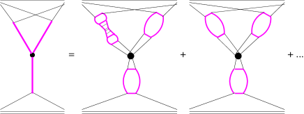
Figure 3: Contributions to the triple-Pomeron vertex from interactions between soft and semi-hard Pomerons.

Basically we shall stay close to the $\pi$-meson dominance picture,[9] where all the vertexes $g_{mn}$ for the transition of $m$ into $n$ Pomerons have been expressed via a single additional constant $r_{3{\mathbb{P}}}$ and where an asymptotic re-summation procedure has been proposed.[18] In particular, for the lowest in $r_{3{\mathbb{P}}}$ contribution with only one multi-Pomeron vertex (Fig. 4)

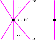
Figure 4: Lowest order enhanced graphs; constituent partons not shown explicitely.

one can obtain, summing over $m,n\geq 1$ and subtracting the term with $m=n=1$ (Pomeron self-coupling):[18]

$$\Delta\chi_{ad}^{(1)(j,k)}(s,b) = \frac{r_{3{\mathbb{P}}}}{\lambda_{j}^{a}\,\lambda_{k}^{d}\,\gamma_{\mathbb{P}}^{3}}\int_{\frac{s_{0}}{s}}^{1}\!\frac{dx_{{\mathbb{P}}}}{x_{{\mathbb{P}}}}\int\!d^{2}b^{\prime}\,\left\{\left[1-e^{-\lambda_{j}^{a}\,\chi_{a{\mathbb{P}}}^{\mathbb{P}}(s_{0}/x_{{\mathbb{P}}},b^{\prime})}\right]\right.$$ (10)

$$\times\left[1-e^{-\lambda_{k}^{d}\,\chi_{d{\mathbb{P}}}^{\mathbb{P}}(x_{{\mathbb{P}}}s,|\vec{b}-\vec{b}^{\prime}|)}\right]$$

$$\left.-\lambda_{j}^{a}\,\lambda_{k}^{d}\;\chi_{a{\mathbb{P}}}^{\mathbb{P}}(s_{0}/x_{{\mathbb{P}}},b^{\prime})\;\chi_{d{\mathbb{P}}}^{\mathbb{P}}(x_{{\mathbb{P}}}s,|\vec{b}-\vec{b}^{\prime}|)\right\},$$

with $\chi_{a{\mathbb{P}}}^{\mathbb{P}}(\hat{s},b^{\prime})\equiv\chi_{a\pi}^{\mathbb{P}}(\hat{s},b^{\prime})$, $\gamma_{\mathbb{P}}=\gamma_{\pi}$; here and below the indexes $j,k$ refer to the diffractive eigenstates of hadrons $a,d$ correspondingly. It is easy to see that in the large $s$, small $b$ limit $\Delta\chi_{ad}^{(1)(j,k)}(s,b)$ is dominated by the last term in the integrand, i.e. by the subtracted self-coupling contribution. Therefore, asymptotically it was sufficient to consider a small sub-set of enhanced graphs, which can be obtained from the one in Fig. 4 iterating multi-Pomeron vertex in $t$-channel. In the “dense” limit re-summation of those diagrams reduces to the sum over subtracted Pomeron self-couplings and, after neglecting the slope of the multi-Pomeron vertex, $R_{\mathbb{P}}^{2}\sim 0$, results in a re-normalization of the Pomeron intercept,[18] $\tilde{\alpha}_{{\mathbb{P}}}(0)=\alpha_{{\mathbb{P}}}(0)-4\pi\,r_{3{\mathbb{P}}}/\gamma_{\mathbb{P}}$.

In this work we also assume an eikonal structure of the multi-Pomeron vertexes, $\gamma_{{\mathbb{P}}-{\mathbb{P}}}^{(m,n)}=r_{3{\mathbb{P}}}\,\gamma_{\mathbb{P}}^{m+n-3}$, but treat $\gamma_{\mathbb{P}}$ as a free parameter and neglect the vertex slope, $R_{\mathbb{P}}^{2}\sim 0$. On the other hand, we neglect a momentum spread of “Pomeron ends” in the vertexes and define the eikonal $\chi_{a{\mathbb{P}}}^{\mathbb{P}}$ as

$$\chi_{a{\mathbb{P}}}^{\mathbb{P}}(\hat{s},b^{\prime})=\int_{s_{0}/\hat{s}}^{1}\!dx^{+}\;N_{a}^{(1)}(x^{+})\;G_{a{\mathbb{P}}}^{\mathbb{P}}(x^{+}\hat{s},b^{\prime}),$$ (11)

where $G_{a{\mathbb{P}}}^{\mathbb{P}}$ is given by Eqs. (5-7), with $d\rightarrow\mathbb{P}$. Correspondingly, for a Pomeron exchanged between two internal vertexes, e.g., in Fig. 5, we just use $G_{{\mathbb{P}}{\mathbb{P}}}^{\mathbb{P}}(s_{0}\,x_{{\mathbb{P}}_{k}}/x_{{\mathbb{P}}_{k+1}},|\vec{b}_{k}-\vec{b}_{k+1}|)$, the latter being defined by Eqs. (5-7) with $ad\rightarrow\mathbb{P}\mathbb{P}$.

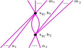
Figure 5: An example of a “loop” graph.

Our goal is to develop a re-summation procedure which assures a smooth transition between the “dilute” (small $s$, large $b$) and “dense” limits and accounts for all essential contributions in both cases. Thus, we shall only neglect “loop” diagrams (Fig. 5) and “chess-board” graphs with more than three vertexes in a horizontal row – Fig. 6.

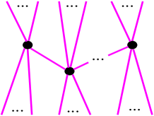
Figure 6: An example of a “chess-board” graph; only three vertexes are shown explicitely.

The neglected diagrams give small contribution at low energies and/or large impact parameters, being proportional to large powers ($\geq 2$) of $r_{3{\mathbb{P}}}$. On the other hand, in the “dense” limit they are strongly suppressed by exponential factors.[18] For the example of Fig. 5, summing over any number $n_{1}$ of Pomerons exchanged between the target and the upper multi-Pomeron vertex (for the other vertex the procedure is similar), we can obtain a factor

$$\sum_{n_{1}=0}^{\infty}\frac{\left[-\lambda_{k}^{d}\,\chi_{d{\mathbb{P}}}^{\mathbb{P}}(x_{{\mathbb{P}}_{1}}s,|\vec{b}-\vec{b}_{1}|)\right]^{n_{1}}}{n_{1}!}=e^{-\lambda_{k}^{d}\,\chi_{d{\mathbb{P}}}^{\mathbb{P}}(x_{{\mathbb{P}}_{1}}s,|\vec{b}-\vec{b}_{1}|)}$$ (12)

We start with obtaining a “fan” diagram contribution $\chi_{a}^{{\rm fan}(j)}$ via a recursive equation – Fig. 7:

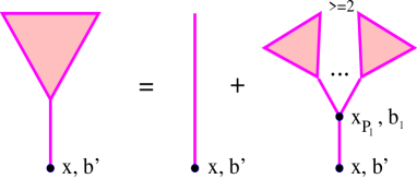
Figure 7: Recursive equation for a “fan” diagram contribution $\chi_{a}^{{\rm fan}(j)}(\hat{s},b^{\prime})$, $\hat{s}=s_{0}/x$.

$$\chi_{a}^{{\rm fan}(j)}\!(\hat{s},b^{\prime}) = \chi_{a{\mathbb{P}}}^{\mathbb{P}}(\hat{s},b^{\prime})-\frac{r_{3{\mathbb{P}}}}{\lambda_{j}^{a}\,\gamma_{\mathbb{P}}^{3}}\int_{\frac{s_{0}}{\hat{s}}}^{1}\!\frac{dx_{{\mathbb{P}}_{1}}}{x_{{\mathbb{P}}_{1}}}\int\!d^{2}b_{1}\,G_{{\mathbb{P}}{\mathbb{P}}}^{\mathbb{P}}(x_{{\mathbb{P}}_{1}}\hat{s},|\vec{b}^{\prime}-\vec{b}_{1}|)$$ (13)

$$\times\sum_{m=2}^{\infty}\,\frac{\left[-\lambda_{j}^{a}\>\chi_{a}^{{\rm fan}(j)}\!(s_{0}/x_{{\mathbb{P}}_{1}},b_{1})\right]^{m}}{m!}$$

$$= \chi_{a{\mathbb{P}}}^{\mathbb{P}}(\hat{s},b^{\prime})+\frac{r_{3{\mathbb{P}}}}{\lambda_{j}^{a}\,\gamma_{\mathbb{P}}^{3}}\int_{\frac{s_{0}}{\hat{s}}}^{1}\!\frac{dx_{{\mathbb{P}}_{1}}}{x_{{\mathbb{P}}_{1}}}\int\!d^{2}b_{1}\;G_{{\mathbb{P}}{\mathbb{P}}}^{\mathbb{P}}(x_{{\mathbb{P}}_{1}}\hat{s},|\vec{b}^{\prime}-\vec{b}_{1}|)$$

$$\times\left[1-e^{-\lambda_{j}^{a}\,\chi_{a}^{{\rm fan}(j)}\!(s_{0}/x_{{\mathbb{P}}_{1}},b_{1})}-\lambda_{j}^{a}\,\chi_{a}^{{\rm fan}(j)}\!(s_{0}/x_{{\mathbb{P}}_{1}},b_{1})\right]$$

Also we introduce a “generalized fan” contribution $\chi_{ad}^{{\rm G-fan}(j,k)}$ via a recursive equation – Fig. 8:

$$\chi_{ad}^{{\rm G-fan}(j,k)}\!(\hat{s},\vec{b}^{\prime},s,\vec{b}) = \chi_{a{\mathbb{P}}}^{\mathbb{P}}(\hat{s},b^{\prime})+\frac{r_{3{\mathbb{P}}}}{\lambda_{j}^{a}\,\gamma_{\mathbb{P}}^{3}}\int_{\frac{s_{0}}{\hat{s}}}^{1}\!\frac{dx_{{\mathbb{P}}_{1}}}{x_{{\mathbb{P}}_{1}}}\int\!d^{2}b_{1}$$ (14)

$$\times G_{{\mathbb{P}}{\mathbb{P}}}^{\mathbb{P}}(x_{{\mathbb{P}}_{1}}\hat{s},|\vec{b}^{\prime}-\vec{b}_{1}|)\,\left\{e^{-\lambda_{k}^{d}\,\chi_{d}^{{\rm fan}(k)}\!(x_{{\mathbb{P}}_{1}}s,|\vec{b}-\vec{b}_{1}|)}\right.$$

$$\times\left[1-e^{-\lambda_{j}^{a}\,\chi_{ad}^{{\rm G-fan}(j,k)}\!(s_{0}/x_{{\mathbb{P}}_{1}},\vec{b}_{1},s,\vec{b})}\right]$$

$$\left.-\lambda_{j}^{a}\>\chi_{ad}^{{\rm G-fan}(j,k)}\!(s_{0}/x_{{\mathbb{P}}_{1}},\vec{b}_{1},s,\vec{b})\right\}$$

The difference between $\chi_{ad}^{{\rm G-fan}(j,k)}$ and $\chi_{a}^{{\rm fan}(j)}$ (Fig. 9) is due to vertexes with both “fans” connected to the projectile and ones connected to the target.

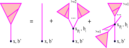
Figure 8: Recursive equation for a “generalized fan” $\chi_{ad}^{{\rm G-fan}(j,k)}(\hat{s},\vec{b}^{\prime},s,\vec{b})$, $\hat{s}=s_{0}/x$.

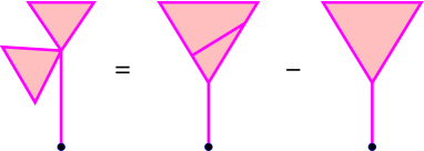
Figure 9: Symbolic notation for the difference between the “generalized fan” and “fan” contributions, $\chi_{ad}^{{\rm G-fan}(j,k)}-\chi_{a}^{{\rm fan}(j)}$.

Now we can obtain total eikonal for an “elementary scattering” process, including all essential enhanced diagram contributions[10] – Fig. 10:

$$\chi_{ad}^{{\rm tot}(j,k)}\!(s,b) = \chi_{ad}^{\mathbb{P}}(s,b)+\frac{r_{3{\mathbb{P}}}}{\lambda_{j}^{a}\,\lambda_{k}^{d}\,\gamma_{\mathbb{P}}^{3}}\int_{\frac{s_{0}}{s}}^{1}\!\!\frac{dx_{{\mathbb{P}}}}{x_{{\mathbb{P}}}}\int\!\!d^{2}b^{\prime}\left\{\left(1-e^{-\lambda_{j}^{a}\,\chi_{ad}^{{\rm G-fan}(j,k)}}\right)\right.$$ (15)

$$\times\left(1-e^{-\lambda_{k}^{d}\,\chi_{da}^{{\rm G-fan}(k,j)}}\right)-\lambda_{j}^{a}\,\lambda_{k}^{d}\>\chi_{ad}^{{\rm G-fan}(j,k)}\,\chi_{da}^{{\rm G-fan}(k,j)}$$

$$-\left[\frac{\lambda_{k}^{d}}{2}\left(\chi_{da}^{{\rm G-fan}(k,j)}-\chi_{d}^{{\rm fan}(k)}\right)\,\left(\left(1-e^{-\lambda_{j}^{a}\,\chi_{ad}^{{\rm G-fan}(j,k)}}\right)\right.\right.$$

$$\left.\times e^{-\lambda_{k}^{d}\,\chi_{d}^{{\rm fan}(k)}}-\lambda_{j}^{a}\,\chi_{ad}^{{\rm G-fan}(j,k)}\right)+\frac{\lambda_{k}^{d}}{2}\left(\chi_{da}^{{\rm G-fan}(k,j)}-\chi_{d{\mathbb{P}}}^{\mathbb{P}}\right)$$

$$\left.\left.\times\left(1-e^{-\lambda_{j}^{a}\,\chi_{a}^{{\rm fan}(j)}}-\lambda_{j}^{a}\,\chi_{a}^{{\rm fan}(j)}\right)\right]-\left[a,j\leftrightarrow d,k\right]\right\}\!,$$

where $\chi_{ad}^{{\rm G-fan}(j,k)}=\chi_{ad}^{{\rm G-fan}(j,k)}(s_{0}/x_{{\mathbb{P}}},\vec{b}^{\prime},s,\vec{b})$, $\chi_{a}^{{\rm fan}(j)}=\chi_{a}^{{\rm fan}(j)}(s_{0}/x_{{\mathbb{P}}},b^{\prime})$, $\chi_{a{\mathbb{P}}}^{\mathbb{P}}=\chi_{a{\mathbb{P}}}^{\mathbb{P}}(s_{0}/x_{{\mathbb{P}}},b^{\prime})$, $\chi_{da}^{{\rm G-fan}(k,j)}=\chi_{da}^{{\rm G-fan}(k,j)}(x_{{\mathbb{P}}}\,s,\vec{b}-\vec{b}^{\prime},s,\vec{b})$, $\chi_{d}^{{\rm fan}(k)}=\chi_{d}^{{\rm fan}(k)}(x_{{\mathbb{P}}}\,s,|\vec{b}-\vec{b}^{\prime}|)$, $\chi_{d{\mathbb{P}}}^{\mathbb{P}}=\chi_{d{\mathbb{P}}}^{\mathbb{P}}(x_{{\mathbb{P}}}\,s,|\vec{b}-\vec{b}^{\prime}|)$.

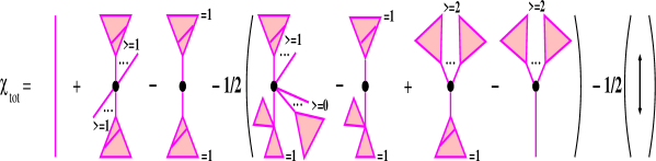
Figure 10: Total hadron-hadron eikonal, including enhanced diagram contributions.

The first term on the r.h.s. in Fig. 10 is a simple Pomeron exchange ($\chi_{ad}^{\mathbb{P}}$); the second graph contains a multi-Pomeron vertex which couples together any number ($\geq 1$) of “generalized fans” connected to the projectile hadron and any number ($\geq 1$) of those connected to the target; the third graph subtracts Pomeron self-coupling contribution; the other terms on the r.h.s. in Fig. 10 correct for double counts of the same diagrams in the second graph. The latter can be verified using Figs. 7–9.

Thus, hadron-hadron elastic scattering amplitude $f_{ad}(s,b)$ can be calculated using Eq. (3), with the simple Pomeron eikonal $\chi_{ad}^{\mathbb{P}}(s,b)$ being replaced by $\chi_{ad}^{\rm{tot}(j,k)}(s,b)$, corresponding to the full set of graphs of Fig. 10. To describe particle production one has to consider unitarity cuts of the amplitude $f_{ad}(s,b)$. Applying AGK cutting rules,[17] one can obtain a set of all cuts of diagrams of Fig. 10, with the eikonal $\chi_{ad}^{\rm{tot-cut}(j,k)}(s,b)\simeq\chi_{ad}^{\rm{tot}(j,k)}(s,b)$, in a similar form, i.e. as a contribution of one cut Pomeron exchange, the latter containing all relevant screening corrections (any number of multi-Pomeron vertexes along the same cut Pomeron line, each vertex having any number but at least one uncut “fan” connected to the projectile or to the target); plus a graph with a multi-Pomeron vertex, which couples together any number ($\geq 1$) of cut “generalized fans” (including diffractive cuts) connected to the projectile hadron and any number ($\geq 1$) of those connected to the target, with all cut Pomeron lines being “dressed” with screening corrections in a similar way; minus double counting contributions.[10] This allows to obtain positively defined probabilities for various configurations of the interaction and to generate the latter via a MC method: starting from sampling (at a given impact parameter $b$ and for given diffractive eigenstates $j,k$) a number of “elementary” particle production processes – according to the eikonal $\chi_{ad}^{\rm{tot-cut}(j,k)}(s,b)$, and choosing a particular sub-configuration for the latter – just one cut Pomeron exchange or a number of cut “generalized fans” emerging from the same multi-Pomeron vertex; in the latter case for each cut “fan” one generates further multi-Pomeron vertexes in an iterative fashion, according to the corresponding probabilities, until the process is terminated. Finally, like in the original linear scheme,[5, 6, 15] one performs energy-momentum sharing between constituent partons of the projectile and of the target, to which cut Pomerons are connected, and finishes with the treatment of particle production from all cut Pomerons. The described scheme easily generalizes to hadron-nucleus and nucleus-nucleus collisions, without introducing any additional parameters. There, screening effects are enhanced by $A$-factors, as different Pomerons belonging to the same enhanced graph may couple to different nucleons of the projectile (target).

4 Cross Sections and Structure Functions

We can also calculate screening corrections to sea quark and gluon PDFs at the initial virtuality scale $Q^{2}_{0}$, which come only from “fan”-type diagrams (neglecting Pomeron “loops”). Thus, parton momentum distributions, being defined in the linear scheme by Eq. (8), are now described by the diagrams of Fig. 7, with the corresponding contributions (Eq. (13)) being summed over hadron $a$ diffractive eigenstates $j$ (with weights $C_{j}^{a}\,\lambda_{j}^{a}$), integrated over $b^{\prime}$, and with the down-most vertex being replaced by the Pomeron-parton coupling:

$$x\,f^{\rm tot}_{I/a}(x,Q_{0}^{2}) = \int\!\!d^{2}b^{\prime}\left\{\int_{x}^{1}\!\!dx^{+}\;N_{a}^{(1)}(x^{+})\;G_{aI}^{{\mathbb{P}}_{\rm soft}}(s_{0}\,x^{+}/x,b^{\prime})\right.$$ (16)

$$+\frac{r_{3{\mathbb{P}}}}{\gamma_{\mathbb{P}}^{3}}\sum_{j}C_{j}^{a}\int_{x}^{1}\!\frac{dx_{{\mathbb{P}}_{1}}}{x_{{\mathbb{P}}_{1}}}\int\!d^{2}b_{1}\>G_{{\mathbb{P}}I}^{{\mathbb{P}}_{\rm soft}}(s_{0}\,x_{{\mathbb{P}}_{1}}/x,|\vec{b}^{\prime}-\vec{b}_{1}|)$$

$$\left.\times\left[1-e^{-\lambda_{j}^{a}\chi_{a}^{{\rm fan}(j)}\!(s_{0}/x_{{\mathbb{P}}_{1}},b_{1})}-\lambda_{j}^{a}\chi_{a}^{{\rm fan}(j)}\!(s_{0}/x_{{\mathbb{P}}_{1}},b_{1})\right]\right\}$$

Similarly one can express diffractive PDFs $f^{\rm DD}_{I/a}(x,x_{{\mathbb{P}}},Q_{0}^{2})$ for a large rapidity gap process in deep inelastic scattering (with $y_{\rm gap}=-\ln x_{{\mathbb{P}}}$) via the contribution of diffractive cuts of “fan” diagrams $\chi_{a}^{{\rm DD}(j)}(\hat{s},x_{{\mathbb{P}}},b^{\prime})$. The latter is obtained cutting the diagrams of Fig. 7 according to the AGK rules and keeping contributions of cuts with the given rapidity gap, which yields again a recursive equation – Fig. 11:

$$\chi_{a}^{{\rm DD}(j)}\!(\hat{s},x_{{\mathbb{P}}},b^{\prime}) = \frac{r_{3{\mathbb{P}}}}{\lambda_{j}^{a}\,\gamma_{\mathbb{P}}^{3}}\int\!d^{2}b_{1}\left\{\frac{1}{2}\left[1-e^{-\lambda_{j}^{a}\,\chi_{a}^{{\rm fan}(j)}\!(s_{0}/x_{{\mathbb{P}}},b_{1})}\right]^{2}\right.$$ (17)

$$\times G_{{\mathbb{P}}{\mathbb{P}}}^{\mathbb{P}}(x_{{\mathbb{P}}}\,\hat{s},|\vec{b}^{\prime}-\vec{b}_{1}|)+\int_{x}^{x_{{\mathbb{P}}}}\!\frac{dx_{{\mathbb{P}}_{1}}}{x_{{\mathbb{P}}_{1}}}\,G_{{\mathbb{P}}{\mathbb{P}}}^{\mathbb{P}}(x_{{\mathbb{P}}_{1}}\hat{s},|\vec{b}^{\prime}-\vec{b}_{1}|)$$

$$\times\lambda_{j}^{a}\,\chi_{a}^{{\rm DD}(j)}\!\left(\frac{s_{0}}{x_{{\mathbb{P}}_{1}}},x_{{\mathbb{P}}},b_{1}\right)\,\left[\exp\left(-\lambda_{j}^{a}\,\chi_{a}^{{\rm fan}(j)}\!\left(\frac{s_{0}}{x_{{\mathbb{P}}_{1}}},b_{1}\right)\right.\right.$$

$$+\int_{x_{{\mathbb{P}}_{1}}}^{x_{{\mathbb{P}}}}\!\frac{dx_{{\mathbb{P}}_{2}}}{x_{{\mathbb{P}}_{2}}}\!\left.\left.\left.\lambda_{j}^{a}\,\chi_{a}^{{\rm DD}(j)}\!\left(\frac{s_{0}}{x_{{\mathbb{P}}_{1}}},x_{{\mathbb{P}}_{2}},b_{1}\right)\right)-1\right]\right\}$$

Correspondingly, the diffractive PDFs $f^{\rm DD}_{I/a}(x,x_{{\mathbb{P}}},Q_{0}^{2})$ are described by the diagrams of Fig. 11, with the corresponding contributions

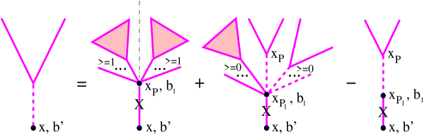
Figure 11: Recursive equation for the diffractive cut $\chi_{a}^{{\rm DD}(j)}\!(\hat{s},x_{{\mathbb{P}}},b^{\prime})$ of “fan” diagrams, $\hat{s}=s_{0}/x$. Cut Pomerons are marked by crosses.

(Eq. (17)) being summed over hadron $a$ diffractive eigenstates, integrated over $b^{\prime}$, and with the down-most vertex being replaced by the Pomeron-parton $I$ coupling, i.e. with the eikonal $G_{{\mathbb{P}}{\mathbb{P}}}^{\mathbb{P}}$ being replaced by $G_{{\mathbb{P}}I}^{{\mathbb{P}}_{\rm soft}}$ (cf. Eqs. (13), (16)).

The obtained parton momentum distributions can be used to calculate total and diffractive structure functions (SFs) $F_{2}$, $F_{2}^{\rm D(3)}$ as

$$F_{2}(x,Q^{2}) = \sum_{I=q,\bar{q}}e_{I}^{2}\,x\,f_{I/p}(x,Q^{2})$$ (18)

$$F_{2}^{\rm D(3)}(x_{{\mathbb{P}}},\beta,Q^{2}) = \sum_{I=q,\bar{q}}e_{I}^{2}\,x\,f^{\rm DD}_{I/p}(x,x_{{\mathbb{P}}},Q^{2}),$$ (19)

where $\beta=x/x_{\mathbb{P}}$ and $f_{I/p}(x,Q^{2})$, $f^{\rm DD}_{I/p}(x,x_{{\mathbb{P}}},Q^{2})$ are obtained evolving the input distributions $f_{I/p}(x,Q_{0}^{2})$, $f^{\rm DD}_{I/p}(x,x_{{\mathbb{P}}},Q_{0}^{2})$ from $Q^{2}_{0}$ to $Q^{2}$ (for valence quark PDFs $q_{v}(x,Q^{2}_{0})$ a parameterized input (GRV94)[20] has been used).

For the cutoff value $Q^{2}_{0}=2$ GeV² the Pomeron parameters have been finally fixed on the basis of experimental data on total hadron-hadron cross sections, elastic scattering slopes, and proton SFs $F_{2}$, $F_{2}^{\rm D(3)}$, in particular, we had $\alpha_{{\mathbb{P}}}(0)=0.205$, $\alpha_{{\mathbb{P}}}^{\prime}(0)=0.09$ GeV^-2, $r_{3{\mathbb{P}}}=0.026$ GeV^-1, $\gamma_{\mathbb{P}}=0.5$ GeV^-1. The obtained behavior of $\sigma_{pp}^{{\rm tot}}(s)$, $F_{2}(x,Q^{2})$, and $F_{2}^{\rm D(3)}(x_{{\mathbb{P}}},\beta,Q^{2})$ is shown in Figs. 12–14.

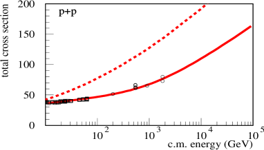
Figure 12: Total $pp$ cross section calculated with and without enhanced diagram contributions – full and dashed curves correspondingly. The compilation of data is from Ref. 21.

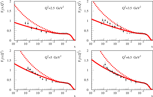
Figure 13: Proton SF $F_{2}(x,Q^{2})$ calculated with and without enhanced graph corrections – full and dashed curves correspondingly. The data are from Refs. 22–24.

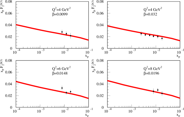
Figure 14: Diffractive proton SF $F_{2}^{D(3)}(x_{{\mathbb{P}}},\beta,Q^{2})$ in low $\beta$ bins compared to preliminary data of ZEUS collaboration (Ref. 25).

In Figs. 12–13 we plot also $\sigma_{pp}^{{\rm tot}}(s)$ and $F_{2}(x,Q^{2})$ as calculated without enhanced diagram contributions, i.e. setting $r_{3{\mathbb{P}}}=0$.

It is noteworthy that in the described scheme the contribution of semi-hard processes to the interaction eikonal can no longer be expressed in the usual factorized form, Eqs. (7), (9). Significant non-factorizable corrections come from graphs where at least one Pomeron is exchanged in parallel to the parton hard process, with the simplest example given by the 1st diagram on the r.h.s. in Fig. 3. In fact, such contributions are of importance to get a consistent description of hadron-hadron cross sections and hadron structure functions. At the same moment, due to the AGK cancellations[17] the above-mentioned non-factorizable graphs do not contribute to inclusive high-$p_{t}$ jet spectra. Single inclusive particle cross sections are defined by diagrams of Fig. 15.

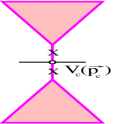
Figure 15: Diagrams contributing to single inclusive cross sections; cut Pomerons are marked by crosses. $V_{c}(\vec{p}_{c})$ is the particle $c$ emission vertex from a cut Pomeron.

In particular, parton jet spectra are thus obtained in the usual factorized form, being defined by the integrand in curly brackets in Eq. (9), with the corresponding PDFs $f^{\rm tot}_{I/a}(x,Q^{2})$ containing “fan” diagram screening corrections.

5 Results for Extensive Air Showers

In general, various features of hadronic interactions contribute to air shower development in a rather non-trivial way. Nevertheless, basic EAS observables are grossly defined by a limited number of macroscopic characteristics of hadron-air collisions: inelastic cross sections $\sigma_{h-\rm{air}}^{\rm{inel}}$ , so-called inelasticities $K_{h-\rm{air}}^{\rm{inel}}$ (relative energy differences between the lab. energies of the initial and the most energetic final particles), and charged particle multiplicities $N_{h-\rm{air}}^{\rm{ch}}$. Indeed, the most fundamental EAS parameter, the position of the shower maximum $X_{\max}$ (atmospheric depth $X$, where the number of charged particles $N_{e^{\pm}}(X)$ reaches its maximal value), is mainly determined by $\sigma_{h-\rm{air}}^{\rm{inel}}$ and $K_{h-\rm{air}}^{\rm{inel}}$. In turn, the number of charged particles $N_{e^{\pm}}$, measured at a given observation level, is strongly correlated with $X_{\max}$. On the other hand, measured muon number $N_{\mu}$ has a much smaller correlation with the shower maximum but depends significantly on $N_{h-\rm{air}}^{\rm{ch}}$.

In Figs. 16–18

Figure 16: Inelastic hadron-air cross sections calculated using QGSJET-II and QGSJET models – full and dashed curves correspondingly.

Figure 17: Inelasticities of hadron-air interactions for QGSJET-II and QGSJET models – full and dashed curves correspondingly.

Figure 18: Multiplicities of charged particles in hadron-air interactions for QGSJET-II and QGSJET models - full and dashed curves.

the predictions of the new model for $\sigma_{h-\rm{air}}^{\rm{inel}}$, $K_{h-\rm{air}}^{\rm{inel}}$, and $N_{h-\rm{air}}^{\rm{ch}}$ are plotted in comparison with the results of the original QGSJET model. The observed different behavior results from a competition of two effects. First of all, non-linear screening corrections reduce the interaction eikonal, slow down the energy increase of hadron-air cross section, compared to the linear scheme with the same Pomeron parameters, and suppress secondary particle production. On the other hand, larger Pomeron intercept and steeper PDFs in QGSJET-II lead to a faster energy increase of the latter quantities. At not too high energies the first effect dominates, resulting in smaller inelasticities and multiplicities. Nevertheless, in very high energy limit the influence of parton distributions prevails and the new model predicts larger values of $K_{h-\rm{air}}^{\rm{inel}}$ and $N_{h-\rm{air}}^{\rm{ch}}$.

Sizably smaller inelasticities of the new model lead to a somewhat deeper position of the shower maximum, compared to the original QGSJET – Fig. 19. As the relative strength of non-linear

Figure 19: Average position of the shower maximum for vertical proton- and iron-induced EAS as calculated with QGSJET-II and QGSJET models – full and dashed curves correspondingly, compared to the data of HIRES collaboration (points) – Ref. 26.

effects is larger for nucleus-nucleus collisions, the difference in $X_{\max}$ is stronger for nucleus-induced air showers. Although the effect is rather moderate at highest energies it changes drastically the interpretation of EAS data: while the predictions of the original QGSJET, being compared to, e.g., HIRES data,[26] are marginally consistent with the assumption of ultra high energy cosmic rays being only protons, this is no longer the case with the new model.

The relative difference between QGSJET-II and QGSJET models for predicted muon number ($E_{\mu}>1$ GeV) at sea level for vertical proton- and iron-induced showers is shown in Fig. 20. In the new model $N_{\mu}$ is significantly smaller, by as much as 30% at highest energies, due to the substantial reduction of $N_{h-\rm{air}}^{\rm{ch}}$ over a wide energy range (see Fig. 18).

Figure 20: Relative $N_{\mu}$-difference ($E_{\mu}>1$ GeV) at sea level between QGSJET-II and QGSJET models for vertical proton- and iron-induced EAS – full and dashed curves.

In general, applying the new model to EAS data reconstruction will change present conclusions concerning cosmic ray composition towards heavier primaries. At the energies in the region of the “knee” of the CR spectrum ($E_{0}\sim 10^{15}-10^{16}$ eV) the obtained changes seem to go in the right direction to improve the agreement with experimental data.[27, 28] However, at highest energies the existing conflict between the composition results obtained with fluorescence light-based measurements and with ground arrays[29] (much heavier composition in the latter case) will aggravate using the new model. Indeed, the first method is mainly based on the measured shower maximum position, whereas in the second case the composition results are obtained from studies of lateral muon densities at ground level. As the predicted reduction of $N_{\mu}$ is much stronger compared to the corresponding effect for $X_{\max}$, the mismatch between the corresponding results is expected to increase.

6 Discussion

The approach presented here offers a possibility to treat non-linear interaction effects explicitely in individual high energy hadron-hadron (hadron-nucleus, nucleus-nucleus) interactions. The latter are described phenomenologically by means of enhanced (Pomeron-Pomeron interaction) diagrams. A re-summation procedure has been worked out which allowed to take into account all essential enhanced graphs, both cut and uncut ones, to obtain positively defined probabilities for various configurations of inelastic interactions, generally, of complicated topology, and to sample such configurations explicitely via a MC method. As an important feature of the proposed scheme, the contribution of semi-hard processes to the interaction eikonal contains an essential non-factorizable part. On the other hand, by virtue of the AGK cancellations,[17] the corresponding diagrams do not contribute to inclusive parton jet spectra. The latter are defined by the usual QCD factorization ansatz, with screening corrections contained in parton momentum distributions.

Compared to other approaches,[7, 30] the described scheme does not require high parton densities to be reached; essential non-linear corrections to the interaction dynamics are consistently taken into account, providing a smooth transition between “dilute” (small energies, large impact parameters) and “dense” regimes and approaching the saturation limit for “soft” ($|q^{2}|<Q^{2}_{0}$) particle production in the latter case. On the other hand, the basic assumption of the scheme – “soft” process dominance of multi-Pomeron vertexes, poses restrictions on its application in the region of high parton densities. Indeed, after reaching parton density saturation at the chosen cutoff scale $Q^{2}_{0}$, one has to account for corresponding effects in the perturbative ($|q^{2}|>Q^{2}_{0}$) parton dynamics, i.e. to take into account “hard” Pomeron-Pomeron coupling. Such a treatment is missing here.

Still, parton saturation is not observed in proton structure functions – Fig. 13. However, in our scheme the continuing increase of PDFs in the low $x$ limit is partly due to the non-zero Pomeron slope, which leads to increasing contribution of proton periphery at small $x$. To investigate the problem in more detail we plot in Fig. 21 gluon momentum distribution for a given impact parameter $x\,G(x,b^{\prime},Q^{2}_{0})$, the latter being defined by the integrand in curly brackets in Eq. (16). As seen from the Figure, at small $b^{\prime}$ the gluon density is indeed close to the saturation at the scale $Q^{2}_{0}$ in the small $x$ limit, signalizing the need for perturbative non-linear corrections.

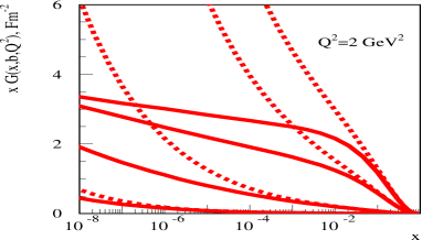
Figure 21: Gluon PDF $x\,G(x,b,Q^{2})$ for a given impact parameter $b$ (from up to bottom $b=0,0.5,1,1.5$ Fm) calculated with and without enhanced graph corrections – full and dashed curves correspondingly.

Applying the approach to air shower simulations we obtained a sizable effect for the calculated EAS characteristics, with the shower maximum getting deeper and with the EAS muon content being significantly reduced. Accounting for perturbative screening corrections (“hard” Pomeron-Pomeron coupling) may enhance corresponding effects. On the other hand, the latter are only significant in the region of high parton densities, i.e. in the “black” region of small impact parameters. Thus, the likely outcome is a further reduction of the interaction multiplicity, without a significant effect on the cross sections and inelasticities, correspondingly, on the predicted shower maximum position. Moreover, a possible loss of coherence in the leading hadron system,[31] which will only affect particle production in the fragmentation region, may have an opposite effect: increasing the inelasticity but having the multiplicity essentially unchanged. Thus, the two effects will lead to further reduction of EAS muon number while having $X_{\max}$ essentially unchanged, or even shifted upwards. Unfortunately, this will worsen the existing contradiction between fluorescence light-based and ground-based results on the cosmic ray composition.[29] There is a hope to clarify the situation with the data of Pierre Auger collaboration,[32] where both experimental techniques are available. The latter can provide an indirect model consistency check at the highest CR energies.

References

- [1] V. N. Gribov, Sov. Phys. JETP 26, 414 (1968); 29, 483 (1969).
- [2] A. B. Kaidalov and K. A. Ter-Martirosian, Phys. Lett. B117, 247 (1982); A. Capella et al., Phys. Rep. 236, 225 (1994).
- [3] J. Ranft, Phys. Rev. D51, 64 (1995).
- [4] K. Werner, Phys. Rep. 232, 87 (1993).
- [5] N. N. Kalmykov and S. S. Ostapchenko, Phys. Atom. Nucl. 56, 346 (1993).
- [6] N. N. Kalmykov, S. S. Ostapchenko, and A. I. Pavlov, Bull. Russ. Acad. Sci. Phys. 58, 1966 (1994); Nucl. Phys. Proc. Suppl. 52B, 17 (1997).
- [7] L. Gribov, E. Levin, and M. Ryskin, Phys. Rep. 100, 1 (1983).
- [8] O. Kancheli, JETP Lett. 18, 465 (1973).
- [9] J. L. Cardy, Nucl. Phys. B75, 413 (1974).
- [10] S. Ostapchenko, In the Proc. of 13th Int. Symp. on Very High Energy Cosmic Ray Interactions, Pylos, Greece, 2004, hep-ph/0412332; article in preparation.
- [11] M. Baker and K. A. Ter-Martirosian, Phys. Rep. 28, 1 (1976).
- [12] H. J. Drescher et al., Phys. Rep. 350, 93 (2001).
- [13] M. L. Good and W. D. Walker, Phys. Rev. 120, 1857 (1960).
- [14] M. Hladik et al., Phys. Rev. Lett. 86, 3506 (2001).
- [15] H. J. Drescher et al., J. Phys. G: Nucl. Part. Phys. 25, L91 (1999); S. Ostapchenko et al., J. Phys. G: Nucl. Part. Phys. 28, 2597 (2002).
- [16] E. Levin and C. I. Tan, hep-ph/9302308.
- [17] V. A. Abramovskii, V. N. Gribov, and O. Kancheli, Sov. J. Nucl. Phys. 18, 308 (1974).
- [18] A. B. Kaidalov, L. A. Ponomarev, and K. A. Ter-Martirosyan, Sov. J. Nucl. Phys. 44, 468 (1986).
- [19] N. N. Nikolaev and B. G. Zakharov, Phys. Lett. B260, 414 (1991).
- [20] M. Gluck, E. Reya, and A. Vogt, Z. Phys. C67, 433 (1995).
- [21] C. Caso et al., Eur. Phys. J. C3, 1 (1998).
- [22] S. Aid et al., H1 Collaboration, Nucl. Phys. B470, 3 (1996).
- [23] M. Derrick et al., ZEUS Collaboration, Z. Phys. C72, 399 (1996).
- [24] M. Arneodo et al., NMC Collaboration, Phys. Lett. B364, 107 (1995).
- [25] F. Goebel, “Measurement of the diffractive contribution to the DIS cross-section using the ZEUS forward plug calorimeter”, DESY-THESIS-2001-049.
- [26] R. U. Abbasi et al., HIRES Collaboration, astro-ph/0407622.
- [27] J. Horandel et al., KASCADE Collaboration, Nucl. Phys. Proc. Suppl. 110, 453 (2002).
- [28] H. Ulrich et al., KASCADE Collaboration, Eur. Phys. J. C33, s944 (2004).
- [29] A. A. Watson, astro-ph/0410514.
- [30] L. D. McLerran and R. Venugopalan, Phys. Rev. D49, 2233 (1994).
- [31] H. J. Drescher, A. Dumitru, and M. Strikman, hep-ph/0408073.
- [32] J. Abraham et al., Pierre Auger Collaboration, Nucl. Instr. Meth. A523, 50 (2004).