Excited Baryons in Large $N_{c}$ QCD

Abstract

This talk reviews recent developments in the use of large $N_{c}$ QCD in the description of baryonic resonances. The emphasis is on the model-independent nature of the approach. Key issues discussed include the spin-flavor symmetry which emerges at large $N_{c}$ and the direct use of scattering observables. The connection to quark model approaches is stressed.

1 Introduction

This talk discusses some recent developments in the description of excited baryons via large $N_{c}$ QCD[1, 4, 2, 3, 5, 6]. The work discussed was principally done in collaboration with Rich Lebed of ASU; two students of mine, Abhi Nellore and Dan Dakin also made substantial contributions and Dan Martin, a student of Rich Lebed’s, also contributed. This talk will be very light on the technical details. I refer you to the original papers for a more detailed description.

To begin with let me motivate why one should look at large $N_{c}$ QCD in this context. The answer is quite simple. Consider the three great lies:

• The check is in the mail.

• Of course, darling, I will respect you in the morning.

• My model is based on QCD.

The perspective of this talk is that the third one of these lies should be lumped with the first two. Let us recall that the good book, a.k.a the Particle Data Book [7], contains an immense amount of information about baryons. But there is no simple systematic way to compute the properties of these states directly from QCD. Virtually all workers in the field use models and the constituent quark model is clearly the standard tool out there. However, as will be discussed below, the constituent quark model has many serious difficulties. Thus it is very important to develop model-independent ways to learn what we can about these states even if these model-independent methods are highly limited. Large $N_{c}$ QCD is such a model-independent tool.

1.1 The Quark Model

The word “quark” has three meanings.

• A nonsense word from James Joyce’s Finnegan’s Wake : “Three quarks for Muster Mark.”

• A fundamental degree of freedom in QCD.

• An effective degree of freedom in the quark model (aliases: the constituent quark model, the naive quark model…)

In many ways the last two are no more closely related than the first two.

The constituent quark model has many problems. In the first place as given it yields stable excited states. To give resonance widths, additional and totally ad hoc dynamics are needed to describe coupling to mesons or quark-antiquark pairs. Thus structure and dynamics are not treated on the same footing. This is highly problematic for descriptions of excited baryons which, after all, are resonances seen in scattering experiments. Secondly, the connection to QCD is totally obscure. The QCD quarks are simply different beasts then constituent quarks. A QCD quark has a mass of $\approx$ 5 MeV; a quark model quark has a mass $\approx$ 300 MeV. Indeed, the role of the quark model in the history of physics is quite ironic. It played a truly essential role in the development of QCD but once QCD was discovered there was no know way to derive the quark model.

Despite these conceptual problems the naive quark model remains the standard picture with which most hadronic physicists think about states, particularly excited states. The reasons for this are clear: The quark model is easy to think about—it is patterned after well-understood atomic physics. Direct QCD calculations for excited states using lattice techniques are extremely difficult and it will be a long while before reliable lattice studies are available. Finally, the quark model works…sort of. Not all states are well described and some predicted states have not been observed.

1.2 Introduction to Large $N_{c}$ QCD

The problem with QCD at low momentum QCD is the absence of a natural expansion parameter. In 1973, just a year after the formalization of QCD, ‘t Hooft proposed that QCD could be generalized from $SU(3)$ to $SU(N_{c})$ and that $1/N_{c}$ can then serve as an expansion parameter[8]. He developed a clever double line diagrammatic method following the color flow and showed that a formal limit exists in which $N_{c}\rightarrow\infty$, $g\rightarrow 0$ with $g^{2}N_{c}$ held fixed. In this expansion planar diagrams of gluons dominate with each nonplanar gluon costing a factor of $N_{c}^{-2}$ and each quark loop counting a factor of $N_{c}^{-1}$. These diagrammatic rules have important implications for correlation functions for operators with the quantum numbers of mesons or glueballs and from these, $N_{c}$ scaling rules can be deduced. Witten generalized the approach to include baryons by arguing that a mean-field picture becomes increasing well justified as $N_{c}\rightarrow\infty$ [9]. Formally this analysis yields, among other rules, the following $N_{c}$ scaling rules:

$$m_{\rm meson} \sim N_{c}^{0}\;\;\;M_{\rm baryon}\sim N_{c}^{1}$$

$$\Gamma_{n-\rm meson} \sim N_{c}^{1-n/2}\;\;\;\;{\rm thus}\;\;\;\Gamma_{3\rm-meson}\sim N_{c}^{-1/2}$$

$$g_{\rm meson-baryon} \sim N_{c}^{1/2}\;\;g_{2\,\rm meson-baryon}\sim N_{c}^{0}$$ (1)

where $\Gamma_{n-\rm meson}$ is an n-meson vertex and $g_{\rm meson-baryon}$ is a coupling constant of a meson to a baryon.

There are important phenomenological consequences from these generic scaling rules which give a cartoon-like description of the real world:

• Baryons are heavy compared to mesons.

• Mesons are weakly interacting among themselves.

• Baryons are strongly coupled to mesons but baryon-meson scattering is order unity.

• OZI rule is qualitatively understood (it becomes exact as $N_{c}\rightarrow\infty$).

• Dominance of two-meson decays when possible,

• Explains non-existence of $qq\overline{q}\overline{q}$ exotics. (They cannot bind at large $N_{c}$).

• Domination of meson and glueball tree graphs in effective theory; helps justify Regge picture.

• Requires the existence of hybrid mesons (e.g., states with quantum numbers of a quark-antiquark and valence glue). [10]

1.3 Spin-Flavor Symmetry For Large $N_{c}$ Baryons

The large $N_{c}$ analysis discussed so far has been generic in the sense that the specific spin and flavor quantum numbers played no special role. As will be seen, for the case of baryons spin and flavor play an exceptionally important role. In particular, a contracted $SU(2N_{f})$ (where $N_{f}$ is the number of degenerate light flavors) emerges for baryons at large $N_{c}$. This symmetry is closely related to the $SU(2N_{f})$ symmetry of the simplest version of the quark model.

The key idea in the derivation of the symmetry is large $N_{c}$ consistency[11, 12]. Suppose one were studying pion-nucleon scattering. The contribution from the direct and crossed Born graphs are proportional to $g_{piNN}^{2}\sim N_{c}$. All non-Born graphs (including the sum of iterated pion exchange) according to Witten’s counting rules scales as $N_{c}^{0}$, apparently yielding a scattering amplitude which scales as $N_{c}^{1}$. However, this violates unitarity. The only way to make the counting consistent is if the Born terms are canceled by other baryons (e.g., the $\Delta$) which are degenerate with the nucleon (for $N_{c}\rightarrow\infty$) and for which there is a conspiracy in the coupling constants.

Such a structure is possible only if the vertices satisfy a set of commutation relations. It turns out that this set of commutation relations is the Lie algebra of contracted $SU(2N_{f})$. Thus, this algebra, and its associated group, becomes exact in the large $N_{c}$ limit. In this write-up, I will spare you details and refer you to the original papers. The key things I would like to stress, however, is that this group structure captures considerable dynamical information. The low-lying baryon states must fall into nearly degenerate multiplets corresponding to representations of the group. Moreover, within the subspace of the states in a representation there is a Wigner-Eckert theorem at work so that all operators can be expressed as c-numbers (i.e. reduced matrix elements) times matrix elements of generators which can be determined entirely from group theoretic considerations. Corrections to this must be of relative order $1/N_{c}$ or smaller.

Now as it happens all the representations of this contracted group are infinite dimensional. The lowest-lying members of the representation are physical and the higher lying states are seen as large $N_{c}$ artifacts. The usual nucleon and $\Delta$ are assumed to be in the lowest representation of the group—this is the only model dependence of the approach. Now it turns out this representation “looks like” states in a naive quark model (for large $N_{c}$) with all quarks in identical s-wave orbitals[13]. They look like the quark model states in the sense that there is a one-to-one mapping between the states in the representation and states in the quark model with the same quantum numbers.

This lowest-lying representation is composed of states which have $I=J$ (where $I$ is the isospin). The lowest two states are identified as the nucleon and $\Delta$. Higher-lying states are seen as $1/N_{c}$ artifacts; the nucleon-$\Delta$ mass splitting goes like $N_{c}^{-1}$. The ratio of matrix elements of operators between different states in the representation are fixed by Clebsch-Gordan coefficients for the group up to corrections which vanish at large $N_{c}$. For example, at large $N_{c}$, $g_{\pi N\Delta}=\frac{3}{2}g_{\pi NN}$. In nature, this relation holds to a few percent so the approach has real predictive power. (In fact this particular comparison works as well as it does in part because this particular relation is “gold-plated” in that it does not acquire any correction correction at order $1/N_{c}$[12, 13].

There is a technical trick introduced by Dashen, Jenkins and Manohar to do the group theory simply[13]. One can map the generators onto a quark model with all quarks in a single s-wave orbital with the generators given by:

$$X_{ia}=\frac{1}{N_{c}}q^{+}\sigma_{i}\tau_{a}q\;\;\;\;\;\;J_{i}=q^{+}\sigma_{i}q\;\;\;\;\;\;T_{a}=q^{+}\tau_{a}q\;;$$ (2)

in the limit $N_{c}\rightarrow\infty$ these generators reproduce the commutation relations of the algebra. Thus, to calculate all of the relevant Clebsches it is sufficient to compute the matrix elements in the quark model. It should be noted here that this does not mean the dynamics is that quark model—this is merely a “poor man’s” way to do group theory.

One key result of the group theory which will play a crucial role for the excited states is the $I=J$ rule. This rule states that all operators which contribute in leading order carry quantum numbers with $I=J$. This rule was originally seen in the Skyrme model[14] but was subsequently derived directly from the group theory of large $N_{c}$ QCD[15]. Operators violating this rule are suppressed by a factor of $N_{c}^{-|I-J|}$.

2 Large $N_{c}$ and Excited Baryons

At first sight it may seem straightforward to simply extend this analysis directly to excited baryons. If the states are fixed by symmetry and the symmetry can be simply encoded in a quark model basis it seems that one can simply create a large $N_{c}$ quark model and automatically get the large $N_{c}$ results. In fact, a number of papers have done just that[16, 17, 18, 19, 20, 21, 22, 23, 24]. There are two conceptual problems associated with this, however. The first is that the derivation of the group theoretic result was only for the space states degenerate with the nucleon at large $N_{c}$ and these excited states are split from the nucleon by order $N_{c}^{0}$. Thus, a priori there is no direct justification for the group structure without redoing the large $N_{c}$ consistency argument. Now as it happens Pirjol and Yan in a technical tour de force did precisely this and showed that a contracted $SU(2N_{f})$ structure arises for the excited states [16].

Despite the beautiful mathematics of ref. [16] it has an underlying conceptual problem: it is based on the scattering of pions off of asymptotic baryon states. However, the excited baryons are not generically stable asymptotic states even at large $N_{c}$. As shown originally by Witten the characteristic width of an excited baryon is $N_{c}^{0}$—they do not become stable at large $N_{c}$[9]. Thus, it is not legitimate to do an analysis based on the assumption that the scattering amplitudes of a pion off of an excited baryon is well defined. This problem could be evaded at least for some class of states if there existed a class of states which for symmetry reasons has a width which goes like $N_{c}^{-1}$. Now as it happens, in reference [16] it is shown that in the context of a simple large $N_{c}$ quark model there are states with a width $\sim N_{c}^{-1}$. However, as discussed in ref. [2], this is only an artifact of the simple quark model and is not a generic large $N_{c}$ result. Thus the straightforward extension of the techniques for the ground band are not justified for excited states.

2.1 Scattering Amplitudes

The key idea that Rich Lebed and I pursued to evade the difficulty that a straightforward extension of the techniques used for the ground band to excited states was to focus directly on physical observables rather than on particular baryon “states”. Recall, that difficulty with focusing on particular excited baryon states is that they are resonances rather than stable states. Moreover, as a practical experimental matter, the only way we know about these state is through scattering experiments. Thus, our first goal is to use large $N_{c}$ methods to understand scattering. As a matter of principle we do not know directly from large $N_{c}$ methods whether QCD has any baryon resonances (or more to the point, any baryon resonances which are narrow enough to observe even if we lived in a truly large $N_{c}$ world). However, if we are able to relate scattering amplitudes in different channels to each other at large $N_{c}$, then we can conclude that if there is a pole in the scattering amplitude at complex energy—i.e., a resonance—in one channel it will have a nearby partner in another.

To see how this works consider for simplicity the case of two-flavored QCD and focus on pion-baryon scattering where the baryon is a ground state baryon (nucleon, $\Delta$). A generic scattering amplitude can be labeled $S_{LL^{\prime}RR^{\prime}IJ}^{\pi}$, where $L$ ($L^{\prime}$) is the initial (final) pion orbital angular momentum, $R$ ($R^{\prime}$) is the initial (final) spin and angular momentum of the baryon, and $I_{s}$, $J_{s}$ is the total isospin and angular momentum in the s-channel. The key thing is that this amplitude is an operator in the space of baryons and, hence, at leading order satisfies the $I=J$ rule (which as a scattering process is a t-channel variable). Since general isospin and angular momentum allows more t-channel amplitudes than the $I=J$ rule does, at large $N_{c}$ QCD the various amplitudes are related. Using standard recoupling identities to go from the t-channel to s-channel [1] yields the following large $N_{c}$ result:

$$S_{LL^{\prime}RR^{\prime}IJ}^{\pi} = \sum_{K}(-1)^{R^{\prime}-R}\sqrt{(2R+1)(2R^{\prime}+1)}$$ (7)

$$(2K+1)\left\{\begin{array}[]{ccc}K&I&J\\ R^{\prime}&L^{\prime}&1\end{array}\right\}\left\{\begin{array}[]{ccc}K&I&J\\ R&L&1\end{array}\right\}s_{KL^{\prime}L}^{\pi},$$

An analogous result can be derived for $\eta$ nucleon scattering.

$$S_{LRJ}^{\eta}=\sum_{K}\sqrt{(2R+1)(2R^{\prime}+1)}(2K+1)\delta_{KL}\,\delta(LRJ)\,s_{K}^{\eta}.$$ (8)

The reason that various scattering amplitudes are linearly related is clear from the structure of eqs. (7) and (8): There are more amplitudes $S_{LL^{\prime}RR^{\prime}IJ}^{\pi}$ than there are $s_{KL^{\prime}L}^{\pi}$ amplitudes, and thus there are linear constraints between them that hold to leading order in the $1/N_{c}$ expansion; similarly, there are more $S_{LRJ}^{\eta}$ amplitudes than $s_{K}^{\eta}$ amplitudes.

Note that in both the $\pi$ and $\eta$ scattering cases there are “reduced” scattering amplitudes $s_{KL^{\prime}L}^{\pi}$ and $s_{K}^{\eta}$. Both of these depend on a variable $K$ which is summed over in the final expression. As will be seen, this $K$ quantum can be used to distinguish resonances.

While these formulae are not new—they were previously derived in the context of the Skyrme model[25]—the present model-independent derivation is. One can algebraically eliminate the reduced matrix elements to obtain relations directly between the physical amplitudes which hold to leading order in $1/N_{c}$. I will refer you to the original papers for an enumeration of all such relations and a test of how well they work. Here for concreteness I focus on one particularly illuminating case of $\pi$-N scattering ($R=R^{\prime}=1/2$) with $L=L^{\prime}=5$ (f-waves). The scattering amplitudes can be denoted in the form $S_{F,2(I+1),2(J+1)}$

$$S_{f,3,7}=\frac{9}{14}S_{f,1,5}+\frac{5)}{14}S_{f,1,7}\;$$ (9)

In fig. 1 the left and right sides of eq. (9) are plotted for both the real and the imaginary parts of amplitudes extracted from the scattering data. It is easy to envision how the two sides can overlap exactly as $N_{c}\rightarrow\infty$.

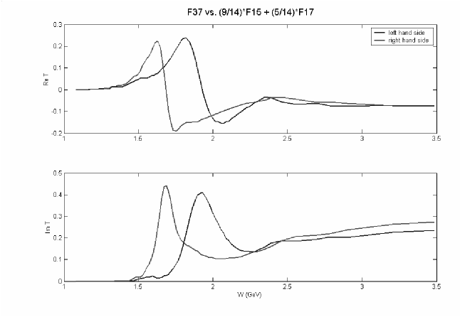
Figure 1: Comparisons of the scattering amplitudes of the right-hand side of eq. (9) with the left-hand side. The upper curve represents the real part while the lower curve represents the imaginary. The amplitudes are extracted from a partial wave extraction of the fit to scattering data [26].

Apart from the fact that they demonstrate the predictive power of the method, the data in fig. 1 also show how resonances are related. Clearly there is a resonance in the F37 channel, since the left-hand side must equal the right-hand side up to $1/N_{c}$ corrections there clearly must also be a resonance in at least one of the channels on the right-hand side and that is exactly what we see. Thus, although I have not shown from first principles that either channel needs to have a resonance, I have demonstrated that if there is a resonance in one channel there will be resonances in other channels which are degenerate up to $1/N_{c}$ corrections.

Before completing a discussion of the degeneracy of resonances and the symmetries that it entails, it is useful to mention at this stage that the method can be generalized and extended. For example one can work at next to leading order (which only has additional predictive power in the reaction $\pi{\rm N}\rightarrow\pi\Delta$)[2] or study $\eta$N scattering, photoprodction reactions[6] or scattering in exotic (pentaquark) channels[4].

2.2 Baryon Resonances

A resonance is a pole in the scattering amplitude at unphysical kinematics. Suppose for the sake of argument that eq. (7) was exact ($1/N_{c}$ corrections were negligible) and that there was a resonance in a particular channel and, hence, a pole in the scattering amplitude at some unphysical point. Such a divergence is only possible if one of the reduced amplitudes itself diverges. Therefore, the existence of a resonance implies a pole in a reduced amplitude. However, a single reduced amplitude contributes to many physical amplitudes. Thus the existence of a resonance in one channel in large $N_{c}$ QCD predicts the existence of a resonance in other channels. Note that not only does this imply the existence of a resonance in the other channels but the existence of a resonance at the same unphysical value for the energy. This means that the resonances are degenerate: large $N_{c}$ QCD predicts the existence of degenerate multiplets of resonances.

A few comments are in order about such multiplets. The first is that position of the resonances for these multiplets are degenerate in the complex plane: thus they are degenerate in both mass and width. This result needs to be taken with a grain of salt, however, due to $1/N_{c}$ corrections. While it is formally true at large $N_{c}$ that the widths and masses will be degenerate, one might expect that for the lowest-lying resonances of physical interest that there might be large $1/N_{c}$ corrections to the widths. The reason for this is simply that for low-lying states the widths are highly sensitive to the available phase space, and small variations in the mass of state due to $1/N_{c}$ corrections can yield large differences in the widths. It is probably better to characterize the widths and coupling constants as being nearly degenerate at large but finite $N_{c}$ rather than the masses and the widths.

Note that these multiplets share a common $L$, $L^{\prime}$ and $K$. The $L$ and $L^{\prime}$ are important in characterizing the incoming and outgoing channels while the $K$ quantum number really characterizes the intrinsic properties of the resonances. Note the existence of degenerate multiplets of states is exactly what one expects if the states fall into representations of some group. In this sense the analysis above implies the existence of an emergent $SU(2N_{f})$ symmetry for the excited states at large $N_{c}$ as well as the ground states. This provides some a posteriori justification for the treatments of refs. [16, 17, 18, 19, 20, 21, 22, 23, 24].

It is important to understand the connection between this approach and the quark model based approach of refs. [17, 18, 19, 20, 21, 22, 23, 24]. On the one hand, as noted above, there is no real a priori justification for the approach. Unlike the analysis of the ground band baryons, for excited baryons the quark model approach is more than just “poor man’s group theory”; it makes real dynamical assumptions including the assumption that the states are stable (or at least narrow at large $N_{c}$ and that some fixed number of quarks are in excited orbitals). Despite this, there is a strong connection between this approach and the model-independent method described above. In particular, the underlying group structure of the quark model implies that if one only includes the leading order operators in the $1/N_{c}$ expansion then the excitation energies in the quark model fall neatly into degenerate multiplets[17, 18, 19, 20, 21, 22, 23, 24]. This fact is not manifestly clear in the treatments of [18, 19, 20, 21, 22, 23, 24] since subleading operators were included at the outset. Moreover, the spin-flavor quantum numbers of these multiplets are in a one-to-one correspondence with those allowed for a particular $K$ multiplets resonant analysis above[1]. Thus, the quark model captures the multiplet structure of the underlying $1/N_{c}$ dynamics.

2.3 Phenomenological Consequence

In the best of all possible worlds, one would see clear evidence for the large $N_{c}$ multiplet structure in the hadronic data with small splittings due to $1/N_{c}$ effects. Alas, in this world things are not so nice. The difficulty is that splittings between multiplets are small compared to the splitting within each multiplet. The reason for this is unclear but is not connected with $1/N_{c}$ physics in any obvious way. To make sense of this situation more analysis is required. A better understanding of how higher-order effects enter is clearly needed and work along this direction is being pursued. Another possible way to see effects is to broaden the analysis to three flavors and see if the effects of the multiplet structure are more apparent there. Again, to do this, systematic higher-order corrections are necessary (this time in $SU(3)$ flavor breaking). Analysis of the $SU(3)$ generalization has begun[5].

There is, however, one place where the large $N_{c}$ analysis has already borne phenomenological fruit and that is the study of decays of negative parity nucleon states. One puzzling aspect of these states is the fact that the N(1520) decays very strongly to the $\eta$N channel and comparatively weakly to the $\pi$N channel (they have very similar branching fractions even though the phase space for $\pi N$ is a factor of  3 greater) while the N(1650) decays very strongly to the $\pi$N channel and very weakly to the $\eta$N channel. This can be easily understood from large $N_{c}$. If one assumes that the states to good approximation fall into $K$ multiplets with small admixtures due to $1/N_{c}$ effects, then this behavior is quite natural. It is easy to see by tracking through the quantum numbers that a pure $K=1$ negative parity nucleon cannot decay into $\eta N$ and a pure $K=0$ negative parity nucleon cannot decay into $\pi N$. Thus if one identifies the N(1520) as (predominantly) a $K=0$ state and the N(1650) as (predominantly) a $K=0$ state, the decay patterns are easily understood.

References

- [1] T.D. Cohen and R.F. Lebed, Phys. Rev. Lett. 91, 012001 (2003); Phys. Rev. D 67, 096008 (2003); Phys. Rev. D 68, 056003 (2003).
- [2] T.D. Cohen, D.C. Dakin, R.F. Lebed, and A. Nellore, Phys. Rev. D 69, 056001 (2004).
- [3] T.D. Cohen, D.C. Dakin, R.F. Lebed, and A. Nellore, Phys. Rev. D 70, 056004 (2004).
- [4] T.D. Cohen and R.F. Lebed, Phys. Lett. B 578, 150 (2004).
- [5] T.D. Cohen, R.F. Lebed Phys. Rev. D 70, 096015 (2004).
- [6] T.D. Cohen, D.C. Dakin, R.F. Lebed, and D.R. Martin, hep-ph/0412294.
- [7] Particle Data Group, Phys. Lett. B 592, 1 (2004).
- [8] G. ’t Hooft Nucl. Phys. B72, 461 (1974).
- [9] E. Witten, Nucl. Phys. B160, 57 (1979).
- [10] T.D. Cohen, Phys. Lett. B 427, 348 (1998).
- [11] J.-L. Gervais and B. Sakita, Phys. Rev. Lett. 52, 87 (1984); Phys. Rev. D 30, 1795 (1984).
- [12] R.F. Dashen and A.V. Manohar, Phys. Lett. B 315, 425 (1993); 315, 438 (1993).
- [13] R.F. Dashen, E. Jenkins, and A.V. Manohar, Phys. Rev. D 49, 4713 (1994).
- [14] M.P. Mattis and M. Mukerjee, Phys. Rev. Lett. 61, 1344 (1988).
- [15] D.B. Kaplan and A.V. Manohar, Phys. Rev. C 56, 76 (1997).
- [16] D. Pirjol and T.-M. Yan, Phys. Rev. D 57, 1449 (1998); Phys. Rev. D 57, 5434 (1998);
- [17] C.D. Carone, H. Georgi, and S. Osofsky, Phys. Lett. B 322, 227 (1994).
- [18] C.E. Carlson, C.D. Carone, J.L. Goity, and R.F. Lebed, Phys. Rev. D 59, 114008 (1999).
- [19] C.E. Carlson, C.D. Carone, J.L. Goity, and R.F. Lebed, Phys. Lett. B 438, 327 (1998).
- [20] C.D. Carone, H. Georgi, L. Kaplan, and D. Morin, Phys. Rev. D 50, 5793 (1994).
- [21] J.L. Goity, Phys. Lett. B 414, 140 (1997).
- [22] C.L. Schat, J.L. Goity, and N.N. Scoccola, Phys. Rev. Lett. 88, 102002 (2002); J.L. Goity, C.L. Schat, and N.N. Scoccola, Phys. Rev. D 66, 114014 (2002).
- [23] C.E. Carlson and C.D. Carone, Phys. Lett. B441, 363 (1998); Phys. Rev. D 58, 053005 (1998).
- [24] C.E. Carlson and C.D. Carone, Phys. Lett. B484, 260 (2000).
- [25] A. Hayashi, G. Eckart, G. Holzwarth, and H. Walliser, Phys. Lett. B147, 5 (1984); M.P. Mattis and M. Karliner, Phys. Rev. D 31, 2833 (1985);M.P. Mattis and M.E. Peskin, Phys. Rev. D 32, 58 (1985);M.P. Mattis, Phys. Rev. Lett. 56, 1103 (1986); Phys. Rev. D 39, 994 (1989); Phys. Rev. Lett. 63, 1455 (1989).
- [26] The data is from SAID and is available at George Washington University’s Center for Nuclear Studies website: http://gwdac.phys.gwu.edu.