Photons in gapless color-flavor-locked quark matter

We calculate the Debye and Meissner masses of a gauge boson in a material consisting of two species of massless fermions that form a condensate of Cooper pairs. We perform the calculation as a function of temperature, for the cases of neutral Cooper pairs and charged Cooper pairs, and for a range of parameters including gapped quasiparticles, and ungapped quasiparticles with both quadratic and linear dispersion relations at low energy.

Our results are relevant to the behavior of photons and gluons in the gapless color-flavor-locked phase of quark matter. We find that the photon’s Meissner mass vanishes, and the Debye mass shows a non-monotonic temperature dependence, and at temperatures of order the pairing gap it drops to a minimum value of order $\sqrt{\alpha}$ times the quark chemical potential. We confirm previous claims that at zero temperature an imaginary Meissner mass can arise from a charged gapless condensate, and we find that at finite temperature this can also occur for a gapped condensate.

1 Introduction

In this paper we calculate the Debye and Meissner masses of a gauge boson propagating through a material consisting of two species of massless charged spin-${\textstyle\frac{1}{2}}$ fermions. We assume that, via an unspecified pointlike attractive interaction, these form an $s$-wave (rotationally invariant) condensate of Cooper pairs, which may be neutral or charged depending on the charges of the fermions. We allow the two species to have chemical potentials ${\bar{\mu}}\pm\delta\mu$, and pairing gap parameter $\Delta$, which is momentum-independent because the interaction is pointlike. As one varies the chemical potential splitting $\delta\mu$ of the two species, the spectrum of fermionic excitations (quasiparticles) changes dramatically:

$$\begin{array}[]{l@{\qquad}l@{\qquad}l}\Delta>\delta\mu&\mbox{Gapped spectrum}&\mbox{e.g.: Fig.~{}\ref{fig:disprel}, dotted line}\\ \Delta=\delta\mu&\mbox{Ungapped quadratic spectrum}&\mbox{e.g.: Fig.~{}\ref{fig:disprel}, solid line}\\ \Delta<\delta\mu&\mbox{Ungapped linear spectrum}&\mbox{e.g.: Fig.~{}\ref{fig:disprel}, dashed line}\\ \end{array}$$ (1.1)

We calculate the zero-momentum current-current correlation function (i.e. the Meissner and Debye masses of the corresponding gauge boson) for all these cases, for both a charged and a neutral condensate, as a function of temperature.

To explain the motivation for this calculation, we give in section 2 a summary of the properties of ultra-dense quark matter, focussing in particular on the gapless color-flavor-locked (gCFL) phase [1], in which all these different cases occur. Our calculation is described in sections 3 and 4, with technical details in an appendix. The results are presented and discussed in sections 5 and 6, with concluding remarks in section 7.

2 Gapless color-flavor-locked quark matter

2.1 Overview of the gCFL phase

The behavior of matter at ultra-high density has been the subject of much theoretical work, and is gradually being constrained by experiments. It is generally agreed that at sufficiently high density, matter will be in a color-flavor-locked (CFL) color-superconducting quark matter phase [2] (for reviews, see Ref. [3]). However, there are major questions about the next phase down in density. Recent work [1] suggests that when the density drops low enough so that the mass of the strange quark can no longer be neglected, there is a continuous phase transition from the CFL phase to a new gapless CFL (gCFL) phase. The two are very different: CFL quark matter is a transparent insulator, with no electrons [4]. Its only light mode is a neutral superfluid mode associated with the breaking of baryon number. In contrast, gCFL quark matter is more like a metal: it has gapless quark modes, and electrons, as well as the superfluid mode.

There are many unanswered theoretical questions about gCFL quark matter. It may be modified by condensation of “kaons” [5]. Also, initial calculations indicate that some of the gluons have imaginary Meissner masses, indicating an instability towards the development of color currents [6, 7, 8]. Our results (section 6) confirm that imaginary Meissner masses are associated with gapless charged condensates. If the gCFL phase turns out to be stable after all, then an experimental question will arise: how could one detect gCFL quark matter in nature. The best opportunity for this is in the core of a neutron star, which achieves densities well above nuclear density, at low temperatures that permit color superconductivity. As we will discuss below, the most characteristic properties of gCFL quark matter are its transport properties. For example, the presence of a gCFL region will have a strong effect on the cooling of a neutron star [9]. Further progress will require the calculation of the interactions among the lightest excitations, and in this paper we will lay the groundwork for such investigations by performing a very general calculation of the behavior of zero-momentum gauge bosons coupled to both neutral and charged Cooper pair condensates.

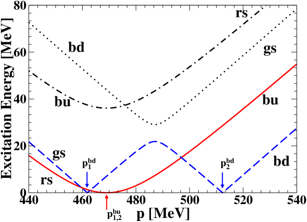
Figure 1: Dispersion relations for some of the quasiquarks in the gapless CFL phase. Note that there is a gapless mode with an approximately quadratic dispersion relation (solid line) as well as two gapless modes with more conventional linear dispersion relations (dashed line), and gapped modes. The labels give the color ($r,g,b$) and flavor ($u,d,s$) content of the quasiparticles.

2.2 Quasiparticle dispersion relations in the gCFL phase

In the gCFL phase, there is a condensate of Cooper pairs of quarks in the color-antisymmetric, flavor-antisymmetric, and Dirac-antisymmetric channel (there is also a insignificant color-symmetric flavor-symmetric component, which we neglect)

$$\langle\psi^{\alpha}_{a}C\gamma_{5}\psi^{\beta}_{b}\rangle\sim\Delta_{1}\epsilon^{\alpha\beta 1}\epsilon_{ab1}\!+\!\Delta_{2}\epsilon^{\alpha\beta 2}\epsilon_{ab2}\!+\!\Delta_{3}\epsilon^{\alpha\beta 3}\epsilon_{ab3}\ .$$ (2.2)

Here $\psi^{\alpha}_{a}$ is a quark of color $\alpha=(r,g,b)$ and flavor $a=(u,d,s)$. The gap parameters $\Delta_{1}$, $\Delta_{2}$ and $\Delta_{3}$ describe down-strange, up-strange and up-down Cooper pairs, respectively.

The gCFL phase is named after its most striking characteristic: the presence of gapless modes in the spectrum of quark excitations above the color-superconducting ground state (3.3). These “gapless quasiquarks” were discussed in Ref. [1], and a sample dispersion relation plot is shown in Fig. 1. This was calculated using a Nambu-Jona-Lasinio model of the strong quark-quark interaction, with a quark chemical potential ${\bar{\mu}}=500~{}{\rm MeV}$, strange quark mass $m_{s}=200~{}{\rm MeV}$ and pairing strength chosen such that at $m_{s}=0$ the CFL gap would be $\Delta_{0}=25~{}{\rm MeV}$ [1]. There are also gapped quasiquarks whose dispersion relations are not shown.

The surprising feature of the gCFL phase is that there is a gapless mode with an approximately quadratic dispersion relation $E(p)\propto(p-p_{F})^{2}$, as well as gapless modes with the more typical linear dispersion relation $E(p)\propto|p-p_{F}|$, and fully gapped modes. The quasiquark spectrum therefore includes all the cases listed in (1.1). The presence of the quadratic gapless mode means that there is a lot of phase space at low energy, in fact the density of states for the quadratic mode diverges as $E\to 0$. We expect this to have dramatic effects on the transport properties, and it has already been pointed out that gCFL quark matter has an unusually large specific heat, which varies as $c_{V}\propto\sqrt{T}$ rather than the usual $c_{V}\propto T$ that is associated with linear gapless dispersion relations. This will alter the late-time cooling of a neutron star in an observable way [9]. To make further progress in studying the transport properties, it will be necessary to understand the dominant (electromagnetic) interactions of the lightest quasiparticles. For this we need the in-medium properties of the photon, which is why calculations of the Debye and Meissner mass of the photon are important.

2.3 Relating our two-species calculation to the gCFL phase

Our calculation explores the case of two species of fermions. This might seem to be a drastic simplification of the gCFL phase, in which there are nine species, but actually the gCFL pairing pattern decomposes into three sectors of two-species pairing and one of three-species pairing. Once pairing has occurred, the dominant interaction between the quasiparticles is mediated by the gauge boson of the remaining unbroken $U(1)_{\tilde{Q}}$ gauge symmetry, whose gauge boson is mostly the original photon, with a small admixture of one of the gluons. The relevant quality of the quasiquark excitations is therefore their ${\tilde{Q}}$ charge, given by ${\tilde{Q}}={\rm diag}({\textstyle\frac{2}{3}},-{\textstyle\frac{1}{3}},-{\textstyle\frac{1}{3}})_{\rm flavor}-{\rm diag}({\textstyle\frac{2}{3}},-{\textstyle\frac{1}{3}},-{\textstyle\frac{1}{3}})_{\rm color}$, not their electromagnetic charge. The pairing pattern and ${\tilde{Q}}$-charges of the quasiparticles are given in Table 1. Each two-species sector has an average chemical potential ${\bar{\mu}}$ and a splitting $\delta\mu$ that arises from the constraint of electrical neutrality and an approximate treatment of the strange quark mass, in which it is treated as a contribution $-M_{s}^{2}/(2{\bar{\mu}})$ to the chemical potential for strangeness. This is known to be a good approximation [10, 11].

species	$ru$	$gd$	$bs$	$gu$	$rd$	$rs$	$bu$	$gs$	$bd$
${\tilde{Q}}$-charge	0	0	0	$+1$	$-1$	$-1$	$+1$	0	0
gap parameter	$\Delta_{1},\Delta_{2},\Delta_{3}$			$\Delta_{3}$		$\Delta_{2}$		$\Delta_{1}$
quasiparticles	gapped			gapped		gapless (quadratic)		gapless (linear)

Table 1: The structure of the gCFL pairing pattern, which decomposes into one sector of three mutually paired species, and three sectors of two species that pair with each other. The ${\tilde{Q}}$ charges of the quarks determine their electromagnetic interactions. Our two-species calculation can be applied to the $gu$-$rd$, $rs$-$bu$, and $gs$-$bd$ sectors.

From Table 1 we see that the transport properties will be dominated by the only electromagnetically interacting light degrees of freedom, namely the $bu$/$rs$ quasiquarks (all the others are either gapped or ${\tilde{Q}}$-neutral) and the electrons. At any nonzero temperature there will be a nonzero density of these ${\tilde{Q}}$-charged particles which may lead to screening of the ${\tilde{Q}}$-electromagnetic fields. Because of their divergent density of states at low energy, we expect the $bu$-$rs$ quasiparticles to dominate this screening. The most direct application of the calculations in this paper is therefore to determine the in-medium properties of the photon in gCFL matter, taking into account the effect of the $bu$/$rs$ quasiquarks. Since the $bu$ and $rs$ quarks have opposite charge, the relevant results are those for a neutral condensate, presented in section 5.

We should note, however, that our calculations of Debye and Meissner masses for charged condensates are also relevant: they can shed light on the behavior of the gauge bosons associated with the broken $SU(3)_{\rm color}$ generators, the gluons. The diagonal color generators can be treated as $U(1)$ gauge fields with their own charge assignments to the quarks, different from the ${\tilde{Q}}$ charges. The fact that they are broken corresponds to the fact that some of the condensates have a net charge. Our two-species calculations show that, as one would expect, when the pairing species have charges that do not cancel each other there is a non-zero Meissner mass for the gauge boson. When the pairing becomes gapless, we find that this Meissner mass becomes imaginary. This confirms existing zero-temperature calculations for the full two-flavor three-color (2SC/g2SC) and three-flavor three-color (CFL/gCFL) pairing patterns [6, 7, 8]. We find that even in the gapped case, turning on a temperature in the appropriate range can cause the Meissner mass to change from real to imaginary.

3 Two-species pairing formalism

In our analysis, we will treat two massless species of fermions (we will refer to them as “quarks”) that pair to yield a condensate

$$\langle\psi_{a}C\gamma_{5}\psi_{b}\rangle=\Delta\epsilon_{ab}\ .$$ (3.3)

By comparison with Eq. (2.2) and table 1 we can see that the $rd$-$gu$, $ru$-$bs$, and $gs$-$bd$ sectors of the CFL or gCFL quark condensate have this structure.

Note that the Dirac charge conjugation matrix $C$ does not connect left-handed with right-handed quarks: the pairing pattern is $\langle\psi_{L}\psi_{L}\rangle$ and $\langle\psi_{R}\psi_{R}\rangle$. Similarly the gauge interactions preserve chiral symmetry, and do not couple left-handed quarks to right-handed quarks. A fermion mass term would couple left-handed to right-handed, but most existing treatments of the gCFL phase work to lowest order in the strange quark mass $M_{s}$, including it via a chemical potential for strangeness $\delta\mu_{s}=-M_{s}^{2}/{\bar{\mu}}$, which also does not couple left-handed quarks to right-handed quarks. To this level of approximation, then, we can treat the left-handed and right-handed quarks as completely decoupled from each other. We can therefore reduce the 4-dimensional Dirac space to a 2-dimensional Weyl space. To treat the quark-quark condensation, which violates fermion number and allows quarks to turn into antiquarks, we need to use Nambu-Gor’kov spinors, which incorporate particles and antiparticles into the same spinor, which doubles the size of our space. So we will work with 8-dimensional chiral spinors $\chi$, which arise from a tensor product of the 2-dimensional Weyl space, the 2-dimensional flavor space, and the Nambu-Gor’kov doubling.

Ignoring electromagnetism, the Lagrangian for our quarks is

$${\cal L}_{0}=\frac{1}{2}\int\chi(p)^{\dagger}S^{-1}(p)\chi(p)\,dp\ ,$$ (3.4)

where the inverse propagator is

$$S^{-1}(p)=\left(\begin{array}[]{c@{\hspace{-2em}}c}(p^{0}+\bar{\mu})\,\bm{1}\otimes\bm{1}+{\vec{p}}\cdot{\vec{\sigma}}\otimes\bm{1}+\delta\mu\,\bm{1}\otimes\sigma_{3}&i\Delta\,\sigma_{2}\otimes\sigma_{1}\\ -i\Delta\,\sigma_{2}^{T}\otimes\sigma_{1}&(p^{0}-\bar{\mu})\,\bm{1}\otimes\bm{1}+{\vec{p}}\cdot{\vec{\sigma}^{T}}\otimes\bm{1}-\delta\mu\bm{1}\otimes\sigma_{3}\end{array}\right)$$ (3.5)

The Nambu-Gor’kov space is shown explicitly in the $2\times 2$ structure of the matrix. In each entry, the first factor in the tensor product lives in the 2-dimensional Weyl (spin) space, and the second factor lives in the 2-dimensional flavor space. The only parameters are the average chemical potential $\bar{\mu}$, the chemical potential splitting $\delta\mu$, and the pairing gap parameter $\Delta$. The off-diagonal terms correspond to the quark pairing: they are proportional to $\Delta$, with a Weyl factor of $\sigma_{2}$ because the Dirac matrix $C={\rm diag}(\sigma_{2},\sigma_{2})$ in the chiral basis, and a flavor factor of $\sigma_{1}$, indicating that the two flavors pair with each other, not with themselves. The on-diagonal terms are standard free fermion terms.

The eight eigenvalues of $S^{-1}$ are

$$p^{0}\pm\sqrt{(|{\vec{p}}|\pm\bar{\mu})^{2}+\Delta^{2}}\pm\delta\mu.$$ (3.6)

The dispersion relations of the quasiquarks are given by the poles in the propagator, i.e. the zeros of $\det(S^{-1})$. With the usual convention that negative energy states are filled, so that all excitations have positive energy, we find

$$E(p)=\left|\sqrt{(|{\vec{p}}|\pm\bar{\mu})^{2}+\Delta^{2}}\pm\delta\mu\right|\ .$$ (3.7)

We see immediately how the relative sizes of $\Delta$ and $\delta\mu$ determine the form of the quasiparticle spectrum,

$$\begin{array}[]{l@{\qquad}l@{\qquad}l}\Delta>\delta\mu&\mbox{Gapped spectrum}&\mbox{($rd$/$gu$ quarks in gCFL)}\\ \Delta=\delta\mu&\mbox{Ungapped quadratic spectrum}&\mbox{($bu$/$rs$ quarks in gCFL)}\\ \Delta<\delta\mu&\mbox{Ungapped linear spectrum}&\mbox{($gs$/$bd$ quarks in gCFL)}\\ \end{array}$$ (3.8)

Actually, in gCFL the $bu$/$rs$ is not precisely gapless, but it is very close: $\delta\mu$ is slightly bigger than $\Delta$,

$$0<\delta\mu-\Delta\ll\delta\mu,\Delta\ll\bar{\mu}\ ,$$ (3.9)

and we will study how the Debye and Meissner masses vary as the temperature is scanned across the full range from $T\ll\delta\mu-\Delta$ to $T\gg{\bar{\mu}}$. Note, however, that because we do not include the physics that leads to the Cooper pairing, $\Delta$ is just a numerical parameter and it does not have the correct $T$-dependence that would send it to zero at $T_{c}\approx 0.57\Delta$. This means that our treatment of pairing is only valid for $T\ll\Delta$ (which is in any case the relevant regime for quark matter in neutron stars) so insofar as our results depend on $\Delta$, they are only valid for $T\ll\Delta$.

4 Gauge boson self-energy

We now discuss the in-medium properties of a gauge boson. These depend on the charges of the two quark species. In general their charges could be $(q_{1},q_{2})=\bar{q}\pm\delta q$, and it turns out that these contributions decouple from one another, so that for both the Debye and Meissner masses we find

$$M^{2}={\bar{q}}^{2}M_{\rm charged}^{2}+(\delta q)^{2}M_{\rm neutral}^{2}$$ (4.10)

Where $M_{\rm charged}$ is the result for a charged condensate in which both flavors have the same charge, and $M_{\rm neutral}$ is the result for a neutral condensate in which the two flavors have opposite charges. Because of this decoupling, we will consider separately the case of a neutral condensate with $(q_{1},q_{2})=(1,-1)$ and a charged condensate with $(q_{1},q_{2})=(1,1)$.

In the Nambu-Gor’kov formalism, the covariant coupling of the fermions to the gauge boson takes the form

$$\frac{1}{2}\,e\,\chi^{T}\Gamma^{\mu}\chi$$ (4.11)

where the gauge coupling is $e$ and $\Gamma^{\mu}$ depends on the charges of the fermions:

$$\begin{array}[]{rcl}\Gamma^{\mu}_{\rm neutral}&=&\left(\begin{array}[]{cc}\sigma^{\mu}\otimes\sigma_{3}&0\\ 0&-{\sigma^{\mu}}^{T}\otimes\sigma_{3}\end{array}\right),\\[8.61108pt] \Gamma^{\mu}_{\rm charged}&=&\left(\begin{array}[]{cc}\sigma^{\mu}\otimes\bm{1}&0\\ 0&-{\sigma^{\mu}}^{T}\otimes\bm{1}\end{array}\right),\\ \sigma^{\mu}&=&\left(\bm{1},{\vec{\sigma}}\right).\end{array}$$ (4.12)

To lowest order in the gauge coupling, the gauge boson self-energy at external momentum $q$ is

$$\Pi_{\rm bare}^{\mu\nu}(q)=e^{2}\int\frac{d^{4}k}{(2\pi)^{4}}{\rm Tr}[\Gamma^{\mu}S(k)\Gamma^{\nu}S(k\!-\!q)].$$ (4.13)

This corresponds to the Feynman diagram shown in Fig. 2. It is to be evaluated using the fermion propagators $S$ obtained by inverting (3.5). The technical details are given in the appendix. Note that our expression (4.13) lacks a factor of ${\textstyle\frac{1}{2}}$ when compared with Eq. (20) of Ref. [12] or Eq. (35) of Ref. [6]. This is because we only include one chirality of fermion in our formalism, so we multiply our result by 2 to obtain the value of $\Pi_{\rm bare}$ for a Dirac fermion with both chiralities.

Figure 2: The Feynman diagram for the lowest-order contribution to the photon self-energy. The internal lines are fermion propagators, obtained by inverting (3.5).

For the transport properties of gCFL quark matter, we are interested in low momentum properties, corresponding to the limit $q\to 0$. For applications to neutron stars we are interested in low temperatures $T\to 0$. We also expect singular behavior as the quark spectrum goes quadratically gapless ($\delta\mu\to\Delta$) as seen in the $bu$/$rs$ modes in gCFL. We have to be careful about the ordering of all these limits. We will take $q\to 0$ first, and then study a range of $T$, both above and below $|\delta\mu-\Delta|$. Our calculations of $\Pi_{\rm bare}$ will yield divergent integrals such as (A.17). To obtain physical results we require a regularization and renormalization prescription. We use a momentum cutoff, and subtract off the vacuum contribution, so that our renormalized results contain only the parts that depend on ${\bar{\mu}}$, $\delta\mu$, and $T$,

$$\Pi(T,\bar{\mu},\delta\mu,\Delta)=\Pi_{\rm bare}(T,\bar{\mu},\delta\mu,\Delta)-\Pi_{\rm bare}(0,0,0,\Delta)\ .$$ (4.14)

The renormalization subtraction term uses the same gap parameter $\Delta$ as the bare contribution. Ultimately, the justification for this is that we then get the correct value for the Meissner mass in the presence of a neutral condensate, namely zero. Other calculations in the literature [12, 6] use a different prescription, $\Pi(T,\bar{\mu},\delta\mu,\Delta)=\Pi_{\rm bare}(T,\bar{\mu},\delta\mu,\Delta)-\Pi_{\rm bare}(0,0,0,0)$, which in our calculation would yield a spurious contribution of order $e^{2}\Delta^{2}$ to the Meissner mass. Such a contribution can be seen in Rischke’s result for the $\lambda_{3}$ gluon mass in two-flavor quark matter (Eq. (115) of Ref. [12]). Rischke guessed that this contribution would be cancelled by other contributions that had been neglected in his calculation. However we do not make any approximations (unlike Rischke we do not try to combine a realistic pairing mechanism with our gauge boson mass calculation, so our computations are simpler than his) and we can see that this term is not cancelled. We think that our prescription is the correct one for the situation that we study, but we do not claim to have provided an a priori justification for it.

5 Debye and Meissner mass for a neutral condensate

5.1 Results

The Debye and Meissner masses are defined by the static long-distance limit of the self energy $\Pi^{\mu\nu}(q)$. (Analysis of the self energy for non-zero $q$ yields interesting information about how the photons resolve the Cooper pairs [13], but we do not attempt such an analysis here.) Taking $q\to 0$ in equations (A.15) and (A.17) and using (4.14), we obtain

$$\lim_{q\to 0}\Pi^{00}(q)=\frac{e^{2}}{\pi^{2}}\int_{0}^{\infty}dk\,k^{2}\Biggl{\{}\frac{d}{dE_{+}}\left[n_{+}(E_{+})+n_{-}(E_{+})\right]+\frac{d}{dE_{-}}\left[n_{+}(E_{-})+n_{-}(E_{-})\right]\Biggr{\}},$$ (5.15)

and

$$\begin{array}[]{rcl}\displaystyle\lim_{q\to 0}\Pi^{ij}(q)&=&\displaystyle 2e^{2}\int\frac{d^{3}k}{(2\pi)^{3}}\Biggl{\{}\hat{k}^{i}\hat{k}^{j}\left[\Delta^{2}\left(\frac{n_{+}(E_{+})+n_{-}(E_{+})}{E_{+}^{3}}+\frac{n_{+}(E_{-})+n_{-}(E_{-})}{E_{-}^{3}}\right)\right.\\ &&\left.\quad\displaystyle+\frac{(k+\bar{\mu})^{2}}{E_{+}^{2}}\frac{d}{dE_{+}}\left[n_{+}(E_{+})+n_{-}(E_{+})\right]+\frac{(k-\bar{\mu})^{2}}{E_{-}^{2}}\frac{d}{dE_{-}}\left[n_{+}(E_{-})+n_{-}(E_{-})\right]\right]\\ &&\displaystyle+(\delta^{ij}-\hat{k}^{i}\hat{k}^{j})\left[\left(1-\frac{k^{2}-\bar{\mu}^{2}+\Delta^{2}}{E_{+}E_{-}}\right)\frac{n_{+}(E_{+})+n_{-}(E_{+})-n_{+}(E_{-})-n_{-}(E_{-})}{E_{+}-E_{-}}\right.\\ &&\displaystyle\left.\quad+\left(1+\frac{k^{2}-\bar{\mu}^{2}+\Delta^{2}}{E_{+}E_{-}}\right)\frac{n_{+}(E_{+})+n_{-}(E_{+})+n_{+}(E_{-})+n_{-}(E_{-})}{E_{+}+E_{-}}\right]\Biggr{\}}\ ,\end{array}$$ (5.16)

where

$$E_{\pm}(k) \equiv \sqrt{(k\pm\bar{\mu})^{2}+\Delta^{2}}\ ,$$ (5.17)

$$n_{\pm}(E) \equiv \displaystyle\left(\exp\Bigl{(}\frac{E\mp\delta\mu}{T}\Bigr{)}+1\right)^{-1}\ .$$ (5.18)

The integral (5.16) evaluates to zero as one would expect: a neutral condensate does not break gauge symmetries, so the Meissner mass is zero,

$$M_{M}^{2}=\frac{1}{2}\lim_{q\to 0}\left(\delta_{ij}-\hat{q}_{i}\hat{q}_{j}\right)\Pi^{ij}(q)=0\ .$$ (5.19)

Note that in obtaining this result it was crucial that we used the correct renormalization subtraction (4.14).

The integral in (5.15) can be evaluated numerically, and also analytically in certain limits. For the Debye mass $M_{D}$, defined by $M_{D}^{2}=-\lim_{q\to 0}\Pi^{00}(q)$, we find

$$M_{D}^{2}=\frac{e^{2}\bar{\mu}^{2}}{\pi^{2}}\left\{\begin{array}[]{ll@{\quad}l}\displaystyle 2\left(1+\frac{\pi^{2}T^{2}}{3\bar{\mu}^{2}}\right),&\delta\mu,\Delta\ll T,\bar{\mu}&\mbox{(a)}\\[8.61108pt] \displaystyle\zeta\sqrt{\frac{2\Delta}{T}},&|\delta\mu-\Delta|\ll T\ll\Delta,\delta\mu\ll\bar{\mu}&\mbox{(b)}\\[8.61108pt] \displaystyle 2\left(1+\frac{\delta\mu^{2}\!-\!\Delta^{2}}{\bar{\mu}^{2}}\right)\frac{\delta\mu}{\sqrt{\delta\mu^{2}\!-\!\Delta^{2}}},&T\ll|\delta\mu-\Delta|,\ \Delta<\delta\mu\ll\bar{\mu}&\mbox{(c)}\\[8.61108pt] \displaystyle\sqrt{\frac{2\pi\Delta}{T}}{\rm e}^{-\frac{\Delta-\delta\mu}{T}},&T\ll|\delta\mu-\Delta|,\ \delta\mu<\Delta\ll\bar{\mu}&\mbox{(d)}\end{array}\right.$$ (5.20)

where the numerical constant $\zeta$ is

$$\zeta=\int_{-\infty}^{\infty}dx\frac{{\rm e}^{-x^{2}}}{\left({\rm e}^{-x^{2}}+1\right)^{2}}\approx 0.673718\ .$$ (5.21)

In the zero temperature limit this becomes

$$M_{D}^{2}(T=0)=\frac{2e^{2}}{\pi^{2}}(\bar{\mu}^{2}+\delta\mu^{2}-\Delta^{2})\frac{\delta\mu}{\sqrt{\delta\mu^{2}-\Delta^{2}}}\theta(\delta\mu-\Delta)\ .$$ (5.22)

5.2 Discussion

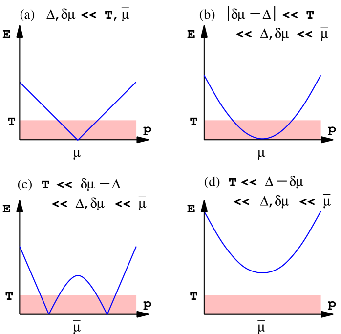
Figure 3: How the dispersion relations of the quasiparticles look at energies of the same order as the temperature, for temperatures coresponding to the cases distinguished in Eq. (5.20). The temperature decreases from (a) to (b) to (c)/(d), and the energy scale stretches accordingly. In each case the shaded region indicates energies $E<T$.

Our result for the Debye mass of a photon passing through a neutral condensate of charged quarks shows a subtle interplay of the limits of small $T$ and small $|\delta\mu-\Delta|$. To understand why the various limits behave so differently, it is useful to recall how the dispersion relations look at energy of order $T$ for the different ranges of temperature distinguished in Eq. (5.20). These are shown in Fig. 3. We will discuss each of the four regimes, bearing in mind that the physical application of our result is to a photon in gCFL quark matter, in which the photon’s in-medium properties are dominated by the $bu$/$rs$ quarks with their near-quadratic gapless dispersion relation.

• corresponds to high temperatures, where the structure in the dispersion relations at scales of order $\Delta,\delta\mu$ is invisible, so the system behaves like free particles with chemical potential $\bar{\mu}$. As noted in section 4, our treatment of the pairing is not valid in this range, but the result turns out to be independent of pairing (i.e. of $\Delta$). Because we have two species we get double the standard one-species result, which is $M_{D}^{2}=e^{2}(\bar{\mu}^{2}/\pi^{2}+T^{2}/3)$ (Ref. [14] Eq. (6.103), in which $m_{D}^{2}=2m^{2}$, see Eq. (7.125)).

• corresponds to temperatures much less than $\delta\mu$ and $\Delta$, but much greater than their difference. This is the typical situation for the $bu$/$rs$ quasiparticles of gCFL matter in a neutron star that is not very old. At energies of the order of $T$ the dispersion relation looks as if it barely touches the momentum axis at a double zero (compare the $bu$/$rs$ line in Fig. 1). This gives the unusual behavior $M_{D}^{2}\propto 1/\sqrt{T}$: the Debye mass increases as $T$ decreases.

• is for temperatures far below the splitting, in the case where $\delta\mu>\Delta$. This corresponds to the $bu$/$rs$ quasiparticles of gCFL quark matter in a very old, cold neutron star. Now a typical thermal fluctuation can resolve the apparent double zero into two separate zeroes. The Debye mass levels out at a constant value as it would for free particles. If $\Delta\ll\delta\mu\ll\bar{\mu}$ then this constant value is the same as in case (a).

• is at a similar temperature to case (c), but for a system where $\delta\mu<\Delta$, so the dispersion relation never actually drops to zero. Relative to a typical thermal fluctuation the quasiparticle gap is a large energy barrier, and $M_{D}$ drops to zero very rapidly with decreasing $T$.

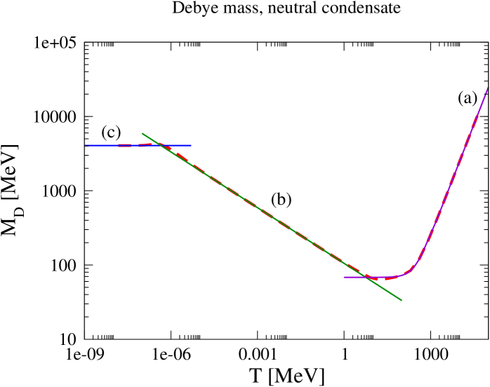
Figure 4: The Debye mass as a function of temperature, for $\bar{\mu}=500~{}{\rm MeV}$, $\delta\mu\approx\Delta=25~{}{\rm MeV}$, $\delta\mu-\Delta=10^{-6}~{}{\rm MeV}$. The heavy dashed line is the numerical result (5.15). The solid lines show the analytic approximations in various regimes of Eq. (5.20), (a), (b), (c). The temperature of a neutron star varies from $\sim 10~{}{\rm MeV}$ in the first seconds after the supernova to $\sim{\rm eV}$ after hundreds of millions of years.

This gives us the temperature dependence for $M_{D}$ shown in Fig. 4. We have chosen values for the parameters that are appropriate for gCFL matter in a neutron star: $e^{2}/(4\pi)=1/137$, $\bar{\mu}=500~{}{\rm MeV}$, $\delta\mu\approx\Delta=25~{}{\rm MeV}$, $\delta\mu-\Delta=10^{-6}~{}{\rm MeV}$ [1]. We evaluate the integral (5.15) numerically, and compare with the analytic approximations of (5.20). Note that $M_{D}$ reaches a very large value at $T=0$. This is because at $T=0$, $M_{D}$ diverges as $\delta\mu/\sqrt{\delta\mu^{2}-\Delta^{2}}$ when $\Delta\to\delta\mu^{-}$ (5.22).

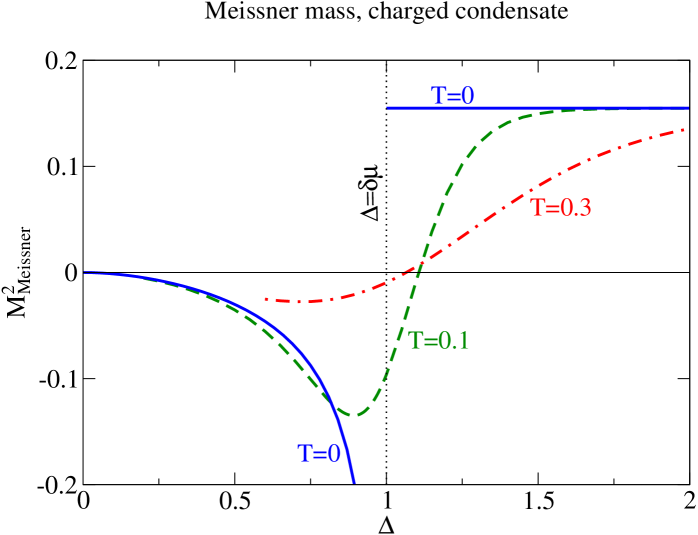
Figure 5: The square of the Meissner mass mass as a function of the gap parameter $\Delta$ at various temperatures, for $\bar{\mu}=5$, $\delta\mu=1$ in arbitrary units. Note how the zero-temperature discontinuity is smoothed out at $T>0$. This means that in the gapped case ($\Delta>\delta\mu$) turning on a temperature in the appropriate range can cause the the Meissner mass to become imaginary.

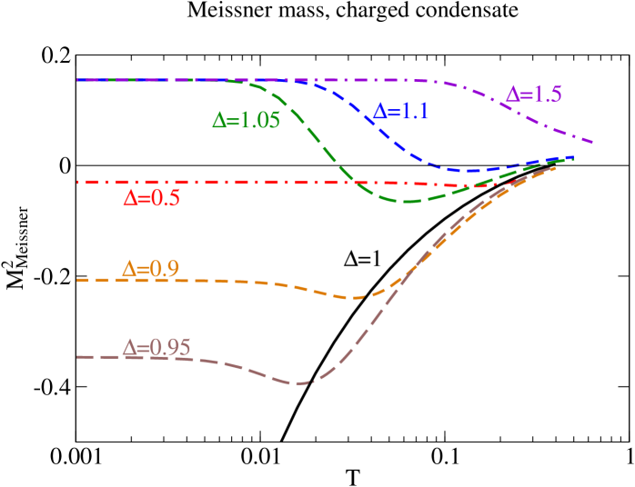
Figure 6: The square of the Meissner mass mass as a function of temperature for various values of the gap parameter, with $\bar{\mu}=5$, $\delta\mu=1$ in arbitrary units. As in Fig. 5, we find that for the gapped case ($\Delta>\delta\mu$), $M_{M}^{2}$ can go from a positive value at $T=0$ to a negative value when $T\gtrsim\Delta-\delta\mu$. The curves stop when $T$ reaches $0.5\Delta$, at which point the temperature-dependence of $\Delta$ can no longer be neglected.

6 Debye and Meissner mass for a charged condensate

6.1 Results

From (A.21) and (A.22), using (4.14), we get

$$\begin{array}[]{rcl}\displaystyle\lim_{q\to 0}\Pi^{00}(q)&=&\displaystyle-\frac{2e^{2}\bar{\mu}^{2}}{\pi^{2}}+\frac{e^{2}}{\pi^{2}}\int_{0}^{\infty}dk\,k^{2}\Biggl{\{}\Delta^{2}\left[\frac{n_{+}(E_{+})+n_{-}(E_{+})}{E_{+}^{3}}+\frac{n_{+}(E_{-})+n_{-}(E_{-})}{E_{-}^{3}}\right]\\ &&\displaystyle+\frac{(k+\bar{\mu})^{2}}{E_{+}^{2}}\frac{d}{dE_{+}}\left[n_{+}(E_{+})+n_{-}(E_{+})\right]+\frac{(k-\bar{\mu})^{2}}{E_{-}^{2}}\frac{d}{dE_{-}}\left[n_{+}(E_{-})+n_{-}(E_{-})\right]\Biggr{\}},\end{array}$$ (6.23)

and

$$\lim_{q\to 0}\Pi^{ij}(q) = \frac{2e^{2}\bar{\mu}^{2}\delta^{ij}}{3\pi^{2}}+2e^{2}\int\frac{d^{3}k}{(2\pi)^{3}}\Biggl{\{}\hat{k}^{i}\hat{k}^{j}\left[\frac{d}{dE_{+}}\left[n_{+}(E_{+})+n_{-}(E_{+})\right]+\frac{d}{dE_{-}}\left[n_{+}(E_{-})+n_{-}(E_{-})\right]\right]$$ (6.24)

$$\quad+(\delta^{ij}-\hat{k}^{i}\hat{k}^{j})\left[\left(1-\frac{k^{2}-\bar{\mu}^{2}-\Delta^{2}}{E_{+}E_{-}}\right)\frac{n_{+}(E_{+})+n_{-}(E_{+})-n_{+}(E_{-})-n_{-}(E_{-})}{E_{+}-E_{-}}\right.$$

$$\qquad\left.+\left(1+\frac{k^{2}-\bar{\mu}^{2}-\Delta^{2}}{E_{+}E_{-}}\right)\frac{n_{+}(E_{+})+n_{-}(E_{+})+n_{+}(E_{-})+n_{-}(E_{-})}{E_{+}+E_{-}}\right]\Biggr{\}}.$$

At arbitrary temperature these integrals can be evaluated numerically. In the zero temperature limit they reduce to

$$\begin{array}[]{rcl}M_{D}^{2}(T=0)&=&\displaystyle\frac{2e^{2}}{\pi^{2}}\Biggl{\{}\bar{\mu}^{2}+\theta(\delta\mu-\Delta)\biggl{(}\delta\mu\sqrt{\delta\mu^{2}-\Delta^{2}}+\Delta^{2}\log\Bigl{(}\frac{\delta\mu-\sqrt{\delta\mu^{2}-\Delta^{2}}}{\Delta}\Bigr{)}\biggr{)}\Biggr{\}}\\[4.30554pt] M_{M}^{2}(T=0)&=&\displaystyle\frac{2e^{2}}{3\pi^{2}}\Biggl{\{}\bar{\mu}^{2}-\theta(\delta\mu-\Delta)\biggl{(}\bar{\mu}^{2}\frac{\delta\mu}{\sqrt{\delta\mu^{2}-\Delta^{2}}}-3\Delta^{2}\log\Bigl{(}\frac{\delta\mu-\sqrt{\delta\mu^{2}-\Delta^{2}}}{\Delta}\Bigr{)}\biggr{)}\Biggr{\}}.\end{array}$$ (6.25)

When $\delta\mu<\Delta$ we recover the well-known result for gluons in the CFL phase, $M_{M}^{2}/M_{D}^{2}=1/3$ [15, 16].

6.2 Discussion

For a given $\delta\mu$, we can calculate the Debye and Meissner masses as a function of temperature $T$ and the gap parameter $\Delta$. The Debye mass is large, $M_{D}\gtrsim\bar{\mu}\gg\Delta$, so we do not discuss it in detail. In the case of the Meissner mass, we can see that at $T=0$ we get an imaginary value when $\delta\mu>\Delta$, i.e. when the system is gapless. This is reminiscent of results found by Shovkovy and Huang and others for gluons in the more complicated cases of g2SC and gCFL quark matter [6, 7, 8]. The square of the Meissner mass as a function of temperature is shown in Figs. 5 and 6. To make these plots we set $\bar{\mu}=5,\ \delta\mu=1$, in arbitrary energy units, and used $e^{2}/(4\pi)=1/137$ as in section 5. The solid “$T=0$” curve in Fig. 5 shows the result of Eq. (6.25): the Meissner mass $M_{M}$ is zero when there is no pairing ($\Delta=0$) . When $\Delta<\delta\mu$, $M_{M}^{2}$ is negative, and diverges to $-\infty$ as $\Delta\to\delta\mu^{-}$. At $\Delta=\delta\mu$, $M_{M}^{2}$ jumps discontinuously to the positive value $2e^{2}\bar{\mu}^{2}/(3\pi^{2})$ that is characteristic of the spontaneous breaking of a gauged symmetry by a charged condensate. It is clear that the limit $\Delta\to\delta\mu$ is singular, with very different behavior according to whether it is taken from above or below. This is quite natural, since for $\Delta>\delta\mu$ the system is always gapped, whereas for $\Delta\leqslant\delta\mu$ it is gapless. We expect that this singular behavior will be smoothed out at any finite nonzero temperature, and this is indeed the case. The curves for $T=0.1$ and $T=0.3$ in Fig. 5 show a smooth transition, over a range $\delta\Delta\sim T$, from the gapless behavior to the gapped behavior.

Essentially the same information is presented in a different way in Fig. 6, where we show the dependence on $T$ for a range of different values of $\Delta$. Again, we fix $\bar{\mu}=5,\ \delta\mu=1$. For $\Delta>\delta\mu$ (gapped system) we see $M_{M}^{2}$ tends to a positive constant as $T\to 0$, whereas for $\Delta<\delta\mu$ we find that $M_{M}^{2}$ tends to a negative value that is large for $\Delta$ just below $\delta\mu$, but tends to zero as $\Delta\to 0$. It is also apparent that the smoothing effect of the non-zero temperature can change a positive $M_{M}^{2}$ into a negative one. This effect is also visible in Fig. 5, and is quite reasonable, given the picture outlined in Fig. 3. If $\Delta>\delta\mu$ then the dispersion relations are gapped, with positive $M_{M}^{2}$ at $T=0$; but if $T>|\delta\mu-\Delta|$ then to within the natural energy resolution ($T$, approximately) the dispersion relation looks quadratically gapless and the Meissner mass will become imaginary. It should be remembered that we have not included any of the pairing dynamics in this calculation, so our gap parameters are independent of temperature. The curves in Figs. 5 and 6 stop when $T$ reaches $0.5\Delta$, at which point the temperature-dependence of $\Delta$ can no longer be neglected.

7 Conclusions

We have calculated the Debye and Meissner masses of a gauge boson in the presence of a condensate of Cooper pairs that involve two species of massless charged spin-${\textstyle\frac{1}{2}}$ fermions. We did not specify any particular pairing mechanism, but simply parameterized the dispersion relations of the quasiparticles using a momentum-independent gap parameter $\Delta$, and individual chemical potentials ${\bar{\mu}}\pm\delta\mu$ for the two species. We allowed the fermions to have arbitrary charge in their coupling to the gauge boson, but found that this reduced to two elementary cases: a neutral condensate (charges $(+1,-1)$), and a charged condensate (charges $(+1,+1)$). Our results for the neutral condensate are presented in section 5 and our results for the charged condensate in section 6.

For the neutral condensate, our results give the in-medium behavior of a very low energy photon (technically, it is the massless ${\tilde{Q}}$ gauge boson that is predominantly the photon with a small admixture of gluon) in the gCFL phase of quark matter. This is dominated by the gapless charged excitations, the $bu$/$rs$ quasiquarks, which form a two-species system of the type that we studied, where the strange quark mass has been treated in lowest order as a contribution to the chemical potential for strangeness. Because the photon coupling is weak, our calculation, which includes only the leading order diagram (Fig. 2), gives the dominant contribution. We find that the Debye mass shows a non-monotonic temperature dependence, dropping to a minimum value of order $\sqrt{\alpha}{\bar{\mu}}$ at temperatures somewhat below the pairing gap. We find that the Meissner mass is zero, as expected for a condensate that does not break the gauge symmetry, and we note that to obtain this result it was necessary to use the renormalization subtraction (4.14), which differs from the one used in the existing literature on quark matter.

For the charged condensate, our results give some insight into the in-medium behavior of gluons in color-superconducting phases. The color-diagonal gluons can be treated as photons with appropriate charge assignments to the various quarks so that the condensates in all three $2\times 2$ sectors of the color-flavor-locked pairing pattern (Table 1) carry net color charge, except that the $rd$-$gu$ condensate is neutral to the $\lambda_{3}$ gluon. We find that there is always a large Debye mass, of order ${\bar{\mu}}^{2}$ or greater. At zero temperature, the square of the Meissner mass is negative for $0<\Delta\leqslant\delta\mu$, diverging to $-\infty$ as $\Delta\to\delta\mu^{-}$, but then jumps discontinuously to a positive value for $\Delta>\delta\mu$. The Meissner mass is therefore imaginary whenever the quasiquark spectrum is gapless, and positive when the spectrum is gapped. At $T>0$ this discontinuity is smoothed out, with interesting consequences. For gapped systems ($\Delta>\delta\mu$) the Meissner mass is real at $T=0$, but it becomes imaginary when $T\gtrsim\Delta-\delta\mu$, as the temperature-smeared dispersion relation is then indistinguishable from a gapless one.

Our charged-condensate results confirm the essential conclusion of Refs. [6] and [7], that charged condensates with gapless excitations are associated with imaginary Meissner mass. In particular, our results for the Meissner mass agree well with those obtained for the diagonal “$\tilde{8}$ gluon” (the combination of a gluon and a photon that is orthogonal to ${\tilde{Q}}$) in Ref. [6]. It is interesting to note that Ref. [6] also finds imaginary Meissner masses for the off-diagonal gluons in the g2SC phase, even in situations where no quasiquark modes are gapless. We cannot offer any insight into this because we only treat diagonal gauge bosons. Also, it is curious that Ref. [7], which treats the gCFL phase, only finds an imaginary Meissner mass for the off-diagonal ($\lambda_{1}$ and $\lambda_{2}$) gluons. Although our 2-species calculation is not directly applicable to the gCFL case, which has multiple pairing sectors (table 1) coupled together by neutrality constraints, our results would lead us to expect that they should have found imaginary Meissner masses for the diagonal $\lambda_{3}$ and $\tilde{8}$ gluons, which both couple to the gapless $bu$-$rs$ and $gs$-$bd$ condensates.

Although we have couched our discussion in terms of gauge boson masses, the quantity that we calculated, the low-momentum current-current two-point function, also has physical meaning if the currents in question are not coupled to gauge fields. In this case $M_{M}^{2}/(e^{2}\Delta^{2})$ is the coefficient of the gradient term in the effective theory of small fluctuations around the ground-state condensate. The fact that we find a negative value when the quasiparticles are gapless indicates an instability towards spontaneous breaking of translational invariance. The nature of the true ground state in gapless color superconductors remains unknown: it could be a mixed phase [18] or a crystalline (LOFF) phase [8]. Since the two-species system shows this instability, it may provide a convenient toy model for investigating the nature of the true ground state.

Acknowledgements

We are grateful to M. Mannarelli for drawing our attention to the temperature-induced imaginary Meissner mass. We have benefitted from discussions with M. Forbes, K. Fukushima, D. Hong, K. Rajagopal, D. Rischke, A. Schmitt, and I. Shovkovy. This research was supported by the Department of Energy under grant number DE-FG02-91ER40628.

Appendix A Calculational details

A.1 Fermion propagator

We calculate the fermion propagator by inverting $S^{-1}$ in (3.5). To doing so, let us write $S$ as a $2\!\times\!2$ matrix

$$S=\left(\begin{array}[]{cc}S_{11}&S_{12}\\ S_{21}&S_{22}\end{array}\right).$$ (A.1)

Since $S$ is Hermitian, we have

$$S_{12}=S_{21}^{{\dagger}}.$$ (A.2)

We may expand each matrix element in $S$ as

$$S_{11} = \alpha^{\prime}(p)\bm{1}\otimes\bm{1}+\beta^{\prime}(p)\bm{1}\otimes\sigma_{3}+\gamma^{\prime}(p){\hat{p}}\cdot{\vec{\sigma}}\otimes\bm{1}+\eta^{\prime}(p){\hat{p}}\cdot{\vec{\sigma}}\otimes\sigma_{3};$$

$$S_{12} = -i\Delta\left[a(p)\bm{1}\otimes\bm{1}+b(p)\bm{1}\otimes\sigma_{3}+c(p){\hat{p}}\cdot{\vec{\sigma}}\otimes\bm{1}+d(p){\hat{p}}\cdot{\vec{\sigma}}\otimes\sigma_{3}\right]\left(\sigma_{2}\otimes\sigma_{1}\right);$$

$$S_{22} = \alpha(p)\bm{1}\otimes\bm{1}+\beta(p)\bm{1}\otimes\sigma_{3}+\gamma(p){\hat{p}}\cdot{\vec{\sigma}^{T}}\otimes\bm{1}+\eta(p){\hat{p}}\cdot{\vec{\sigma}^{T}}\otimes\sigma_{3}.$$ (A.3)

After a lengthy calculation, we have

$$a(p) = \frac{1}{4D_{1}(p)}+\frac{1}{4D_{2}(p)}+\frac{1}{4D_{3}(p)}+\frac{1}{4D_{4}(p)}$$

$$b(p) = \frac{1}{4D_{1}(p)}+\frac{1}{4D_{2}(p)}-\frac{1}{4D_{3}(p)}-\frac{1}{4D_{4}(p)}$$

$$c(p) = \frac{1}{4D_{1}(p)}-\frac{1}{4D_{2}(p)}+\frac{1}{4D_{3}(p)}-\frac{1}{4D_{4}(p)}$$

$$d(p) = \frac{1}{4D_{1}(p)}-\frac{1}{4D_{2}(p)}-\frac{1}{4D_{3}(p)}+\frac{1}{4D_{4}(p)},$$ (A.4)

$$\alpha(p) = \frac{p^{0}+\delta\mu+|{\vec{p}}|+\bar{\mu}}{4D_{1}(p)}+\frac{p^{0}+\delta\mu-|{\vec{p}}|+\bar{\mu}}{4D_{2}(p)}+\frac{p^{0}-\delta\mu+|{\vec{p}}|+\bar{\mu}}{4D_{3}(p)}+\frac{p^{0}-\delta\mu-|{\vec{p}}|+\bar{\mu}}{4D_{4}(p)}$$

$$\beta(p) = -\frac{p^{0}+\delta\mu+|{\vec{p}}|+\bar{\mu}}{4D_{1}(p)}-\frac{p^{0}+\delta\mu-|{\vec{p}}|+\bar{\mu}}{4D_{2}(p)}+\frac{p^{0}-\delta\mu+|{\vec{p}}|+\bar{\mu}}{4D_{3}(p)}+\frac{p^{0}-\delta\mu-|{\vec{p}}|+\bar{\mu}}{4D_{4}(p)}$$

$$\gamma(p) = -\frac{p^{0}+\delta\mu+|{\vec{p}}|+\bar{\mu}}{4D_{1}(p)}+\frac{p^{0}+\delta\mu-|{\vec{p}}|+\bar{\mu}}{4D_{2}(p)}-\frac{p^{0}-\delta\mu+|{\vec{p}}|+\bar{\mu}}{4D_{3}(p)}+\frac{p^{0}-\delta\mu-|{\vec{p}}|+\bar{\mu}}{4D_{4}(p)}$$

$$\eta(p) = \frac{p^{0}+\delta\mu+|{\vec{p}}|+\bar{\mu}}{4D_{1}(p)}-\frac{p^{0}+\delta\mu-|{\vec{p}}|+\bar{\mu}}{4D_{2}(p)}-\frac{p^{0}-\delta\mu+|{\vec{p}}|+\bar{\mu}}{4D_{3}(p)}+\frac{p^{0}-\delta\mu-|{\vec{p}}|+\bar{\mu}}{4D_{4}(p)},$$

and

$$\alpha^{\prime}(p) = \frac{p^{0}+\delta\mu-|{\vec{p}}|-\bar{\mu}}{4D_{1}(p)}+\frac{p^{0}+\delta\mu+|{\vec{p}}|-\bar{\mu}}{4D_{2}(p)}+\frac{p^{0}-\delta\mu-|{\vec{p}}|-\bar{\mu}}{4D_{3}(p)}+\frac{p^{0}-\delta\mu+|{\vec{p}}|-\bar{\mu}}{4D_{4}(p)}$$

$$\beta^{\prime}(p) = \frac{p^{0}+\delta\mu-|{\vec{p}}|-\bar{\mu}}{4D_{1}(p)}+\frac{p^{0}+\delta\mu+|{\vec{p}}|-\bar{\mu}}{4D_{2}(p)}-\frac{p^{0}-\delta\mu-|{\vec{p}}|-\bar{\mu}}{4D_{3}(p)}-\frac{p^{0}-\delta\mu+|{\vec{p}}|-\bar{\mu}}{4D_{4}(p)}$$

$$\gamma^{\prime}(p) = \frac{p^{0}+\delta\mu-|{\vec{p}}|-\bar{\mu}}{4D_{1}(p)}-\frac{p^{0}+\delta\mu+|{\vec{p}}|-\bar{\mu}}{4D_{2}(p)}+\frac{p^{0}-\delta\mu-|{\vec{p}}|-\bar{\mu}}{4D_{3}(p)}-\frac{p^{0}-\delta\mu+|{\vec{p}}|-\bar{\mu}}{4D_{4}(p)}$$

$$\eta^{\prime}(p) = \frac{p^{0}+\delta\mu-|{\vec{p}}|-\bar{\mu}}{4D_{1}(p)}-\frac{p^{0}+\delta\mu+|{\vec{p}}|-\bar{\mu}}{4D_{2}(p)}-\frac{p^{0}-\delta\mu-|{\vec{p}}|-\bar{\mu}}{4D_{3}(p)}+\frac{p^{0}-\delta\mu+|{\vec{p}}|-\bar{\mu}}{4D_{4}(p)},$$

where

$$D_{1}(p) = (p^{0}+\delta\mu)^{2}-(|{\vec{p}}|+\bar{\mu})^{2}-\Delta^{2}$$

$$D_{2}(p) = (p^{0}+\delta\mu)^{2}-(|{\vec{p}}|-\bar{\mu})^{2}-\Delta^{2}$$

$$D_{3}(p) = (p^{0}-\delta\mu)^{2}-(|{\vec{p}}|+\bar{\mu})^{2}-\Delta^{2}$$

$$D_{4}(p) = (p^{0}-\delta\mu)^{2}-(|{\vec{p}}|-\bar{\mu})^{2}-\Delta^{2}.$$ (A.7)

A.2 Matsubara frequency sums

To compute $\Pi_{\rm bare}^{\mu\nu}$, we need do evaluate the 4-dimensional momentum-space integral. At finite temperature, the $k_{0}$ integral becomes a Matsubara frequency sum, in which we replace $k^{0}$ by $i\omega_{n}$, and $\int dk^{0}$ by $2\pi T\sum_{\omega_{n}}$. Because quarks are fermions, they obey antiperiodic temporal boundary conditions, and the Matsubara frequencies are

$$\omega_{n}=\frac{1}{T}(2n+1)\pi,\qquad n\in\mathbb{Z}.$$ (A.8)

To evaluate the frequency sums, we use the following result (Eq. (5.77) in Ref. [14]):

$$T\sum_{\omega_{n}}\frac{1}{(i\omega_{n}+\delta\mu)^{2}+E_{1}^{2}}\,\frac{1}{(i\omega_{n}-i\omega+\delta\mu)^{2}+E_{2}^{2}}$$ (A.9)

$$= \frac{1}{4E_{1}E_{2}}\left[\frac{f_{-}(E_{1})-f_{-}(E_{2})}{i\omega+E_{1}-E_{2}}-\frac{f_{+}(E_{1})-f_{+}(E_{2})}{i\omega-E_{1}+E_{2}}\right.$$

$$\qquad\left.+\frac{1-f_{-}(E_{1})-f_{+}(E_{2})}{i\omega+E_{1}+E_{2}}-\frac{1-f_{+}(E_{1})-f_{-}(E_{2})}{i\omega-E_{1}-E_{2}}\right],$$

where with positive $E$, the functions $f_{\pm}$ are defined as

$$f_{\pm}(sE)\equiv\frac{1}{{\rm e}^{\frac{sE\mp\delta\mu}{T}}+1},\qquad s=\pm 1.$$ (A.10)

From Eq. (5.76) in Ref. [14], we obtain another useful formula

$$T\sum_{\omega_{n}}\frac{1}{i\omega_{n}+\delta\mu+s_{1}E_{1}}\frac{1}{i(\omega_{n}-\omega)+\delta\mu+s_{2}E_{2}}=\frac{f_{-}(s_{1}E_{1})-f_{-}(s_{2}E_{2})}{i\omega+s_{1}E_{1}-s_{2}E_{2}},\quad s_{1},s_{2}=\pm 1.$$ (A.11)

To apply these formulas directly, we need to use the method of partial fractions to convert expressions with $k^{0}$ in the numerator to expressions with $k^{0}$ appearing only in the denominator. A typical example is

$$\frac{(k^{0}+\delta\mu)(k^{0}-q^{0}+\delta\mu)}{D_{1}(k)D_{1}(k\!-\!q)}$$ (A.12)

$$= \frac{1}{4D_{1}(k)D_{1}(k\!-\!q)}\left\{\left[k^{0}+\delta\mu+\sqrt{(|\vec{k}|+\bar{\mu})^{2}+\Delta^{2}}\right]+\left[k^{0}+\delta\mu-\sqrt{(|\vec{k}|+\bar{\mu})^{2}+\Delta^{2}}\right]\right\}$$

$$\quad\times\left\{\left[k^{0}-q^{0}+\delta\mu+\sqrt{(|\vec{k}-\vec{q}|+\bar{\mu})^{2}+\Delta^{2}}\right]+\left[k^{0}-q^{0}+\delta\mu-\sqrt{(|\vec{k}-\vec{q}|+\bar{\mu})^{2}+\Delta^{2}}\right]\right\}$$

$$= \frac{1}{4}\Biggl{[}\frac{1}{k^{0}+\delta\mu+\sqrt{(|\vec{k}|+\bar{\mu})^{2}+\Delta^{2}}}\frac{1}{k^{0}-q^{0}+\delta\mu+\sqrt{(|\vec{k}-\vec{q}|+\bar{\mu})^{2}+\Delta^{2}}}$$

$$\quad+\frac{1}{k^{0}+\delta\mu+\sqrt{(|\vec{k}|+\bar{\mu})^{2}+\Delta^{2}}}\frac{1}{k^{0}-q^{0}+\delta\mu-\sqrt{(|\vec{k}-\vec{q}|+\bar{\mu})^{2}+\Delta^{2}}}$$

$$\quad+\frac{1}{k^{0}+\delta\mu-\sqrt{(|\vec{k}|+\bar{\mu})^{2}+\Delta^{2}}}\frac{1}{k^{0}-q^{0}+\delta\mu+\sqrt{(|\vec{k}-\vec{q}|+\bar{\mu})^{2}+\Delta^{2}}}$$

$$\quad+\frac{1}{k^{0}+\delta\mu-\sqrt{(|\vec{k}|+\bar{\mu})^{2}+\Delta^{2}}}\frac{1}{k^{0}-q^{0}+\delta\mu-\sqrt{(|\vec{k}-\vec{q}|+\bar{\mu})^{2}+\Delta^{2}}}\Biggr{]}.$$

With the integrand in this form, the frequency sum can be evaluated.

A.3 Neutral condensate

We substitute the fermion propagator into the expression for the photon self-energy (4.13) with $\Gamma^{\mu}_{\rm neutral}$ in (4.12). The zero-zero component is

$$\Pi_{\rm bare}^{00} = e^{2}\int\frac{d^{4}k}{(2\pi)^{4}}\Biggl{\{}\left[1+{\hat{k}}\cdot(\widehat{k\!-\!q})\right]\frac{(k^{0}+\delta\mu)(k^{0}-q^{0}+\delta\mu)+\left(|{\vec{k}}|+\bar{\mu}\right)\left(|{\vec{k}}-{\vec{q}}|+\bar{\mu}\right)+\Delta^{2}}{D_{1}(k)D_{1}(k\!-\!q)}$$ (A.13)

$$\qquad+\left[1-{\hat{k}}\cdot(\widehat{k\!-\!q})\right]\frac{(k^{0}+\delta\mu)(k^{0}-q^{0}+\delta\mu)-\left(|{\vec{k}}|+\bar{\mu}\right)\left(|{\vec{k}}-{\vec{q}}|-\bar{\mu}\right)+\Delta^{2}}{D_{1}(k)D_{2}(k\!-\!q)}$$

$$\qquad+(\delta\mu\to\delta\mu)(\bar{\mu}\to-\bar{\mu})+(\delta\mu\to-\delta\mu)(\bar{\mu}\to\bar{\mu})+(\delta\mu\to-\delta\mu)(\bar{\mu}\to-\bar{\mu})\Biggr{\}},$$

where $(\delta\mu\to\pm\delta\mu)(\bar{\mu}\to\pm\bar{\mu})$ means terms as the first two terms with $\delta\mu$ replaced by $\pm\delta\mu$ and $\bar{\mu}$ replaced by $\pm\bar{\mu}$.

The spatial components of the photon self-energy are

$$\Pi_{\rm bare}^{ij} = e^{2}\int\frac{d^{4}k}{(2\pi)^{4}}\Biggl{\{}$$ (A.14)

$$\quad\delta^{ij}\left[\left(1-{\hat{k}}\cdot(\widehat{k\!-\!q})\right)\frac{(k^{0}+\delta\mu)(k^{0}-q^{0}+\delta\mu)+\left(|{\vec{k}}|+\bar{\mu}\right)\left(|{\vec{k}}-{\vec{q}}|+\bar{\mu}\right)-\Delta^{2}}{D_{1}(k)D_{1}(k\!-\!q)}\right.$$

$$\qquad\left.+\left(1+{\hat{k}}\cdot(\widehat{k\!-\!q})\right)\frac{(k^{0}+\delta\mu)(k^{0}-q^{0}+\delta\mu)-\left(|{\vec{k}}|+\bar{\mu}\right)\left(|{\vec{k}}-{\vec{q}}|-\bar{\mu}\right)-\Delta^{2}}{D_{1}(k)D_{2}(k\!-\!q)}\right]$$

$$\quad+\left[{\hat{k}}^{i}(\widehat{k\!-\!q})^{j}+(\widehat{k\!-\!q})^{i}{\hat{k}}^{j}\right]\left[\frac{(k^{0}+\delta\mu)(k^{0}-q^{0}+\delta\mu)+\left(|{\vec{k}}|+\bar{\mu}\right)\left(|{\vec{k}}-{\vec{q}}|+\bar{\mu}\right)-\Delta^{2}}{D_{1}(k)D_{1}(k\!-\!q)}\right.$$

$$\qquad\left.-\frac{(k^{0}+\delta\mu)(k^{0}-q^{0}+\delta\mu)-\left(|{\vec{k}}|+\bar{\mu}\right)\left(|{\vec{k}}-{\vec{q}}|-\bar{\mu}\right)-\Delta^{2}}{D_{1}(k)D_{2}(k\!-\!q)}\right]$$

$$\quad+(\bar{\mu}\to-\bar{\mu})$$

$$\quad+i\epsilon^{ijl}\Biggl{[}\left({\hat{k}}_{l}-(\widehat{k\!-\!q})_{l}\right)\left(-\frac{(k^{0}+\delta\mu)(k^{0}-q^{0}+\delta\mu)+\left(|{\vec{k}}|+\bar{\mu}\right)\left(|{\vec{k}}-{\vec{q}}|+\bar{\mu}\right)-\Delta^{2}}{D_{1}(k)D_{1}(k\!-\!q)}\right.$$

$$\qquad\quad\left.+\frac{(k^{0}+\delta\mu)(k^{0}-q^{0}+\delta\mu)+\left(|{\vec{k}}|-\bar{\mu}\right)\left(|{\vec{k}}-{\vec{q}}|-\bar{\mu}\right)-\Delta^{2}}{D_{2}(k)D_{2}(k\!-\!q)}\right)$$

$$\qquad+\left({\hat{k}}_{l}+(\widehat{k\!-\!q})_{l}\right)\left(-\frac{(k^{0}+\delta\mu)(k^{0}-q^{0}+\delta\mu)-\left(|{\vec{k}}|+\bar{\mu}\right)\left(|{\vec{k}}-{\vec{q}}|+\bar{\mu}\right)-\Delta^{2}}{D_{1}(k)D_{2}(k\!-\!q)}\right.$$

$$\qquad\quad\left.+\frac{(k^{0}+\delta\mu)(k^{0}-q^{0}+\delta\mu)-\left(|{\vec{k}}|-\bar{\mu}\right)\left(|{\vec{k}}-{\vec{q}}|-\bar{\mu}\right)-\Delta^{2}}{D_{2}(k)D_{1}(k\!-\!q)}\right)\Biggr{]}$$

$$\quad+(\delta\mu\to-\delta\mu)\Biggr{\}},$$

where $(\bar{\mu}\to-\bar{\mu})$ and $(\delta\mu\to-\delta\mu)$ means a duplication of all previous terms with $\bar{\mu}$ replaced by $-\bar{\mu}$ or $\delta\mu$ replaced by $-\delta\mu$.

Performing the frequency sums using (A.9) and (A.11), we obtain the zero-zero component of the photon self-energy:

$$\begin{array}[]{rl}\displaystyle\Pi_{\rm bare}^{00}=\frac{e^{2}}{4}\int\frac{d^{3}k}{(2\pi)^{3}}\Bigl{\{}&\left[1+{\hat{k}}\cdot(\widehat{k\!-\!q})\right]\left[1+f_{+,+}^{(1)}(k,p)\right]u_{+,+}(k,p)\\[4.30554pt] +&\left[1+{\hat{k}}\cdot(\widehat{k\!-\!q})\right]\left[1-f_{+,+}^{(1)}(k,p)\right]v_{+,+}(k,p)\\[4.30554pt] +&\left[1-{\hat{k}}\cdot(\widehat{k\!-\!q})\right]\left[1+f_{+,-}^{(1)}(k,p)\right]u_{+,-}(k,p)\\[4.30554pt] +&\left[1-{\hat{k}}\cdot(\widehat{k\!-\!q})\right]\left[1-f_{+,-}^{(1)}(k,p)\right]v_{+,-}(k,p)\\ +&(\delta\mu\to\delta\mu)(\bar{\mu}\to-\bar{\mu})+(\delta\mu\to-\delta\mu)(\bar{\mu}\to\bar{\mu})\\ +&(\delta\mu\to-\delta\mu)(\bar{\mu}\to-\bar{\mu})\Bigr{\}},\end{array}$$ (A.15)

where

$$\begin{array}[]{rcl}f_{r,s}^{(1)}(k,q)&\equiv&\displaystyle\frac{\left(r|{\vec{k}}|+\bar{\mu}\right)\left(s|{\vec{k}}-{\vec{q}}|+\bar{\mu}\right)+\Delta^{2}}{E_{r}(k)E_{s}(k\!-\!q)},\\[8.61108pt] u_{r,s}(k,q)&\equiv&\displaystyle\frac{n_{-}[E_{r}(k)]-n_{-}[E_{s}(k\!-\!q)]}{q^{0}+E_{r}(k)-E_{s}(k\!-\!q)}-\frac{n_{+}[E_{r}(k)]-n_{+}[E_{s}(k\!-\!q)]}{q^{0}-E_{r}(k)+E_{s}(k\!-\!q)},\\[8.61108pt] v_{r,s}(k,q)&\equiv&\displaystyle\frac{1-n_{+}[E_{r}(k)]-n_{-}[E_{s}(k\!-\!q)]}{q^{0}-E_{r}(k)-E_{s}(k\!-\!q)}-\frac{1-n_{-}[E_{r}(k)]-n_{+}[E_{s}(k\!-\!q)]}{q^{0}+E_{r}(k)+E_{s}(k\!-\!q)},\\[8.61108pt] &\lx@intercol(r=\pm 1,\quad s=\pm 1)\hfil\lx@intercol\end{array}$$ (A.16)

For the spatial components, we obtain

$$\Pi_{\rm bare}^{ij} = \frac{e^{2}}{4}\int\frac{d^{3}k}{(2\pi)^{3}}\Bigl{(}$$ (A.17)

$$\left\{\delta^{ij}\left[1-{\hat{k}}\cdot(\widehat{k\!-\!q})\right]+\left[{\hat{k}}^{i}(\widehat{k\!-\!q})^{j}+(\widehat{k\!-\!q})^{i}{\hat{k}}^{j}\right]-i\epsilon^{ijl}\left[{\hat{k}}_{l}-(\widehat{k\!-\!q})_{l}\right]\right\}$$

$$\qquad\times\Bigl{\{}\left[1+f_{+,+}^{(2)}(k,q)\right]u_{+,+}(k,q)+\left[1-f_{+,+}^{(2)}(k,q)\right]v_{+,+}(k,q)\Bigr{\}}$$

$$+\left\{\delta^{ij}\left[1-{\hat{k}}\cdot(\widehat{k\!-\!q})\right]+\left[{\hat{k}}^{i}(\widehat{k\!-\!q})^{j}+(\widehat{k\!-\!q})^{i}{\hat{k}}^{j}\right]+i\epsilon^{ijl}\left[{\hat{k}}_{l}-(\widehat{k\!-\!q})_{l}\right]\right\}$$

$$\qquad\times\Bigl{\{}\left[1+f_{-,-}^{(2)}(k,q)\right]u_{-,-}(k,q)+\left[1-f_{-,-}^{(2)}(k,q)\right]v_{-,-}(k,q)\Bigr{\}}$$

$$+\left\{\delta^{ij}\left[1+{\hat{k}}\cdot(\widehat{k\!-\!q})\right]-\left[{\hat{k}}^{i}(\widehat{k\!-\!q})^{j}+(\widehat{k\!-\!q})^{i}{\hat{k}}^{j}\right]-i\epsilon^{ijl}\left[{\hat{k}}_{l}+(\widehat{k\!-\!q})_{l}\right]\right\}$$

$$\qquad\times\Bigl{\{}\left[1+f_{+,-}^{(2)}(k,q)\right]u_{+,-}(k,q)+\left[1-f_{+,-}^{(2)}(k,q)\right]v_{+,-}(k,q)\Bigr{\}}$$

$$+\left\{\delta^{ij}\left[1+{\hat{k}}\cdot(\widehat{k\!-\!q})\right]-\left[{\hat{k}}^{i}(\widehat{k\!-\!q})^{j}+(\widehat{k\!-\!q})^{i}{\hat{k}}^{j}\right]+i\epsilon^{ijl}\left[{\hat{k}}_{l}+(\widehat{k\!-\!q})_{l}\right]\right\}$$

$$\qquad\times\Bigl{\{}\left[1+f_{-,+}^{(2)}(k,q)\right]u_{-,+}(k,q)+\left[1-f_{-,+}^{(2)}(k,q)\right]v_{-,+}(k,q)\Bigr{\}}$$

$$+(\delta\mu\to-\delta\mu)\Bigr{)},$$

where

$$f_{r,s}^{(2)}(k,q)\equiv\frac{\left(r|{\vec{k}}|+{\bar{\mu}}\right)\left(s|{\vec{k}}-{\vec{q}}|+{\bar{\mu}}\right)-\Delta^{2}}{E_{r}(k)E_{s}(k\!-\!q)}.$$ (A.18)

Now we can send the external momentum $q\to 0$, to obtain integral expressions for the Debye and Meissner masses (see section 5).

A.4 Charged condensate

In the formalism we are using here, the only difference between the neutral case and charged case is the sign in front of $\Delta^{2}$ in the numerators. If we change all the signs of $\Delta^{2}$ in the numerators in the previous subsection and leave the denominators unchanged, we will obtain the correct formulas for the photon self energy in the presence of a charged condensate.

The zero-zero component of the photon self-energy is

$$\Pi_{\rm bare}^{00} = e^{2}\int\frac{d^{4}k}{(2\pi)^{4}}\Biggl{\{}\left[1+{\hat{k}}\cdot(\widehat{k\!-\!q})\right]\frac{(k^{0}+\delta\mu)(k^{0}-q^{0}+\delta\mu)+\left(|{\vec{k}}|+\bar{\mu}\right)\left(|{\vec{k}}-{\vec{q}}|+\bar{\mu}\right)-\Delta^{2}}{D_{1}(k)D_{1}(k\!-\!q)}$$ (A.19)

$$\qquad+\left[1-{\hat{k}}\cdot(\widehat{k\!-\!q})\right]\frac{(k^{0}+\delta\mu)(k^{0}-q^{0}+\delta\mu)-\left(|{\vec{k}}|+\bar{\mu}\right)\left(|{\vec{k}}-{\vec{q}}|-\bar{\mu}\right)-\Delta^{2}}{D_{1}(k)D_{2}(k\!-\!q)}$$

$$\qquad+(\delta\mu\to\delta\mu)(\bar{\mu}\to-\bar{\mu})+(\delta\mu\to-\delta\mu)(\bar{\mu}\to\bar{\mu})+(\delta\mu\to-\delta\mu)(\bar{\mu}\to-\bar{\mu})\Biggr{\}}.$$

The spatial components of the photon self-energy are

$$\Pi_{\rm bare}^{ij} = e^{2}\int\frac{d^{4}k}{(2\pi)^{4}}\Biggl{\{}$$ (A.20)

$$\quad\delta^{ij}\left[\left(1-{\hat{k}}\cdot(\widehat{k\!-\!q})\right)\frac{(k^{0}+\delta\mu)(k^{0}-q^{0}+\delta\mu)+\left(|{\vec{k}}|+\bar{\mu}\right)\left(|{\vec{k}}-{\vec{q}}|+\bar{\mu}\right)+\Delta^{2}}{D_{1}(k)D_{1}(k\!-\!q)}\right.$$

$$\qquad\left.+\left(1+{\hat{k}}\cdot(\widehat{k\!-\!q})\right)\frac{(k^{0}+\delta\mu)(k^{0}-q^{0}+\delta\mu)-\left(|{\vec{k}}|+\bar{\mu}\right)\left(|{\vec{k}}-{\vec{q}}|-\bar{\mu}\right)+\Delta^{2}}{D_{1}(k)D_{2}(k\!-\!q)}\right]$$

$$\quad+\left[{\hat{k}}^{i}(\widehat{k\!-\!q})^{j}+(\widehat{k\!-\!q})^{i}{\hat{k}}^{j}\right]\left[\frac{(k^{0}+\delta\mu)(k^{0}-q^{0}+\delta\mu)+\left(|{\vec{k}}|+\bar{\mu}\right)\left(|{\vec{k}}-{\vec{q}}|+\bar{\mu}\right)+\Delta^{2}}{D_{1}(k)D_{1}(k\!-\!q)}\right.$$

$$\qquad\left.-\frac{(k^{0}+\delta\mu)(k^{0}-q^{0}+\delta\mu)-\left(|{\vec{k}}|+\bar{\mu}\right)\left(|{\vec{k}}-{\vec{q}}|-\bar{\mu}\right)+\Delta^{2}}{D_{1}(k)D_{2}(k\!-\!q)}\right]$$

$$\quad+(\bar{\mu}\to-\bar{\mu})$$

$$\quad+i\epsilon^{ijl}\Biggl{[}\left({\hat{k}}_{l}-(\widehat{k\!-\!q})_{l}\right)\left(-\frac{(k^{0}+\delta\mu)(k^{0}-q^{0}+\delta\mu)+\left(|{\vec{k}}|+\bar{\mu}\right)\left(|{\vec{k}}-{\vec{q}}|+\bar{\mu}\right)+\Delta^{2}}{D_{1}(k)D_{1}(k\!-\!q)}\right.$$

$$\qquad\quad\left.+\frac{(k^{0}+\delta\mu)(k^{0}-q^{0}+\delta\mu)+\left(|{\vec{k}}|-\bar{\mu}\right)\left(|{\vec{k}}-{\vec{q}}|-\bar{\mu}\right)+\Delta^{2}}{D_{2}(k)D_{2}(k\!-\!q)}\right)$$

$$\qquad+\left({\hat{k}}_{l}+(\widehat{k\!-\!q})_{l}\right)\left(-\frac{(k^{0}+\delta\mu)(k^{0}-q^{0}+\delta\mu)-\left(|{\vec{k}}|+\bar{\mu}\right)\left(|{\vec{k}}-{\vec{q}}|+\bar{\mu}\right)+\Delta^{2}}{D_{1}(k)D_{2}(k\!-\!q)}\right.$$

$$\qquad\quad\left.+\frac{(k^{0}+\delta\mu)(k^{0}-q^{0}+\delta\mu)-\left(|{\vec{k}}|-\bar{\mu}\right)\left(|{\vec{k}}-{\vec{q}}|-\bar{\mu}\right)+\Delta^{2}}{D_{2}(k)D_{1}(k\!-\!q)}\right)\Biggr{]}$$

$$\quad+(\delta\mu\to-\delta\mu)\Biggr{\}}.$$

To perform the frequency sum we can take the neutral-condensate results and interchange $f_{r,s}^{(1)}(k,p)$ and $f_{r,s}^{(2)}(k,p)$. Thus we obtain

$$\begin{array}[]{rl}\displaystyle\Pi_{\rm bare}^{00}=\frac{e^{2}}{4}\int\frac{d^{3}k}{(2\pi)^{3}}\Bigl{\{}&\left[1+{\hat{k}}\cdot(\widehat{k\!-\!q})\right]\left[1+f_{+,+}^{(2)}(k,p)\right]u_{+,+}(k,p)\\[4.30554pt] +&\left[1+{\hat{k}}\cdot(\widehat{k\!-\!q})\right]\left[1-f_{+,+}^{(2)}(k,p)\right]v_{+,+}(k,p)\\[4.30554pt] +&\left[1-{\hat{k}}\cdot(\widehat{k\!-\!q})\right]\left[1+f_{+,-}^{(2)}(k,p)\right]u_{+,-}(k,p)\\[4.30554pt] +&\left[1-{\hat{k}}\cdot(\widehat{k\!-\!q})\right]\left[1-f_{+,-}^{(2)}(k,p)\right]v_{+,-}(k,p)\\ +&(\delta\mu\to\delta\mu)(\bar{\mu}\to-\bar{\mu})+(\delta\mu\to-\delta\mu)(\bar{\mu}\to\bar{\mu})\\ +&(\delta\mu\to-\delta\mu)(\bar{\mu}\to-\bar{\mu})\Bigr{\}},\end{array}$$ (A.21)

and

$$\Pi_{\rm bare}^{ij} = \frac{e^{2}}{4}\int\frac{d^{3}k}{(2\pi)^{3}}\Bigl{(}$$ (A.22)

$$\left\{\delta^{ij}\left[1-{\hat{k}}\cdot(\widehat{k\!-\!q})\right]+\left[{\hat{k}}^{i}(\widehat{k\!-\!q})^{j}+(\widehat{k\!-\!q})^{i}{\hat{k}}^{j}\right]-i\epsilon^{ijl}\left[{\hat{k}}_{l}-(\widehat{k\!-\!q})_{l}\right]\right\}$$

$$\qquad\times\Bigl{\{}\left[1+f_{+,+}^{(1)}(k,q)\right]u_{+,+}(k,q)+\left[1-f_{+,+}^{(1)}(k,q)\right]v_{+,+}(k,q)\Bigr{\}}$$

$$+\left\{\delta^{ij}\left[1-{\hat{k}}\cdot(\widehat{k\!-\!q})\right]+\left[{\hat{k}}^{i}(\widehat{k\!-\!q})^{j}+(\widehat{k\!-\!q})^{i}{\hat{k}}^{j}\right]+i\epsilon^{ijl}\left[{\hat{k}}_{l}-(\widehat{k\!-\!q})_{l}\right]\right\}$$

$$\qquad\times\Bigl{\{}\left[1+f_{-,-}^{(1)}(k,q)\right]u_{-,-}(k,q)+\left[1-f_{-,-}^{(1)}(k,q)\right]v_{-,-}(k,q)\Bigr{\}}$$

$$+\left\{\delta^{ij}\left[1+{\hat{k}}\cdot(\widehat{k\!-\!q})\right]-\left[{\hat{k}}^{i}(\widehat{k\!-\!q})^{j}+(\widehat{k\!-\!q})^{i}{\hat{k}}^{j}\right]-i\epsilon^{ijl}\left[{\hat{k}}_{l}+(\widehat{k\!-\!q})_{l}\right]\right\}$$

$$\qquad\times\Bigl{\{}\left[1+f_{+,-}^{(1)}(k,q)\right]u_{+,-}(k,q)+\left[1-f_{+,-}^{(1)}(k,q)\right]v_{+,-}(k,q)\Bigr{\}}$$

$$+\left\{\delta^{ij}\left[1+{\hat{k}}\cdot(\widehat{k\!-\!q})\right]-\left[{\hat{k}}^{i}(\widehat{k\!-\!q})^{j}+(\widehat{k\!-\!q})^{i}{\hat{k}}^{j}\right]+i\epsilon^{ijl}\left[{\hat{k}}_{l}+(\widehat{k\!-\!q})_{l}\right]\right\}$$

$$\qquad\times\Bigl{\{}\left[1+f_{-,+}^{(1)}(k,q)\right]u_{-,+}(k,q)+\left[1-f_{-,+}^{(1)}(k,q)\right]v_{-,+}(k,q)\Bigr{\}}$$

$$+(\delta\mu\to-\delta\mu)\Bigr{)}.$$

Now we can send the external momentum $q\to 0$, to obtain integral expressions for the Debye and Meissner masses (see section 6).

References

- [1] M. Alford, C. Kouvaris and K. Rajagopal, Phys. Rev. Lett. 92, 222001 (2004) [arXiv:hep-ph/0311286]; M. Alford, C. Kouvaris and K. Rajagopal, arXiv:hep-ph/0406137.
- [2] M. Alford, K. Rajagopal and F. Wilczek, Nucl. Phys. B537, 443 (1999) [hep-ph/9804403].
- [3] K. Rajagopal and F. Wilczek, hep-ph/0011333. M. G. Alford, Ann. Rev. Nucl. Part. Sci. 51 (2001) 131 [hep-ph/0102047]. D. H. Rischke, Prog. Part. Nucl. Phys. 52, 197 (2004) [nucl-th/0305030]. T. Schäfer, hep-ph/0304281. S. Reddy, Acta Phys. Polon. B 33, 4101 (2002) [arXiv:nucl-th/0211045].
- [4] K. Rajagopal and F. Wilczek, Phys. Rev. Lett. 86, 3492 (2001) [hep-ph/0012039].
- [5] A. Kryjevski and D. Yamada, arXiv:hep-ph/0407350; A. Kryjevski and T. Schafer, arXiv:hep-ph/0407329.
- [6] M. Huang and I. A. Shovkovy, arXiv:hep-ph/0408268.
- [7] R. Casalbuoni, R. Gatto, M. Mannarelli, G. Nardulli and M. Ruggieri, arXiv:hep-ph/0410401.
- [8] I. Giannakis and H. C. Ren, arXiv:hep-ph/0412015.
- [9] M. Alford, P. Jotwani, C. Kouvaris, J. Kundu and K. Rajagopal, arXiv:astro-ph/0411560.
- [10] K. Fukushima, C. Kouvaris and K. Rajagopal, arXiv:hep-ph/0408322.
- [11] I. A. Shovkovy, S. B. Ruester and D. H. Rischke, arXiv:nucl-th/0411040.
- [12] D. H. Rischke, Phys. Rev. D 62, 034007 (2000) [arXiv:nucl-th/0001040].
- [13] D. F. Litim and C. Manuel, Phys. Rev. D 64, 094013 (2001) [arXiv:hep-ph/0105165].
- [14] M. Le Bellac, Thermal Field Theory, Cambridge, 1996.
- [15] D. H. Rischke, Phys. Rev. D 62, 054017 (2000) [arXiv:nucl-th/0003063].
- [16] A. Schmitt, Q. Wang and D. H. Rischke, Phys. Rev. D 69, 094017 (2004) [arXiv:nucl-th/0311006].
- [17] A. Schmitt, personal communication.
- [18] S. Reddy and G. Rupak, arXiv:nucl-th/0405054.