Non-Gaussianity from Instant and Tachyonic Preheating

Abstract:

We study non-Gaussianity in two distinct models of preheating: instant and tachyonic. In instant preheating non-Gaussianity is sourced by the local terms generated through the coupled perturbations of the two scalar fields. We find that the non-Gaussianity parameter is given by $f_{NL}^{\phi}\sim 2g<{\cal O}(1)$, where $g$ is a coupling constant, so that instant preheating is unlikely to be constrained by WMAP or Planck. In the case of tachyonic preheating non-Gaussianity arises solely from the instability of the tachyon matter and is found to be large. We find that for single field inflation the present WMAP data implies a bound $V_{0}^{1/4}/M_{P}\leq 10^{-4}$ on the scale of tachyonic instability. We argue that the tachyonic preheating limits are useful also for string-motivated inflationary models.

1 Introduction

Preheating, first realized in [1] and worked out in detail in Refs. [2, 3, 4], is an interesting possibility for obtaining a thermal Universe after the end of inflation. Preheating is a non-perturbative phenomenon and perhaps the most efficient way of transferring the inflaton energy density into other degrees of freedom. Without preheating the inflaton would have to decay perturbatively and slowly, thereby requiring a long time scale for the thermalization of the inflaton decay products (for recent discussions, see [5]).

The simplest realization of preheating is obtained if the inflaton condensate has a coupling $g^{2}\varphi^{2}\sigma^{2}$, where $\varphi$ is the inflaton and $\sigma$ is another scalar field. Then during the coherent oscillations of $\varphi$ a resonant production of $\sigma$ quanta can take place due to a temporary vacuum instability. The occupation number of $\sigma$ field increases gradually while the fluctuations in $\sigma$ increase exponentially. An important observation is that during this phase gravitational (metric) fluctuations also get amplified at super-Hubble scales [6, 7] (for a general treatment of first order linear perturbation theory, see [8])

The growth of metric fluctuations is of great interest because of the potential observational consequences. In particular, during inflation the growth of the second order metric fluctuations leads to an enhancement of the non-Gaussianity parameter $f_{NL}^{\phi}$ of the CMB (for a review of non-Gaussianity, see [9]). In our recent paper [10] we considered a particular preheating scenario where in comparison with the inflaton, the dynamics of $\sigma$ was assumed to have negligible impact on metric fluctuations. We estimated the second order metric fluctuations following [11, 12] and found that $f_{NL}^{\phi}$ grows exponentially with a rate that depends on the number of inflaton oscillations. (This is a generic result and applies also to the case of supersymmetric flat directions, which could provide an alternative scenario for reheating the Universe [13]). The result suggests that non-Gaussianity may provide an important test of preheating scenario, and in the present paper we shall demonstrate that this is indeed so.

Non-Gaussianities can also arise after inflation [14] when the energy in the inflaton condensate is transferred to other degrees of freedom. Such a situation arises during preheating as we shall now argue. Let us focus on two different cases. First, let us note that the inflaton could decay non-perturbatively during just one oscillation only. This is simple to understand for example in a chaotic type model with $V\sim m^{2}\varphi^{2}/2$. There inflation ends at $\varphi\sim M_{P}$ and the field rolls down towards its global minimum. However, by virtue of the coupling, $g^{2}\varphi^{2}\sigma^{2}$, the $\sigma$ field obtains an effective mass $m_{\sigma}^{2}=g^{2}\varphi^{2}$. Initially, as long as $|\dot{m}_{\sigma}|\ll m_{\sigma}^{2}$, the fluctuations in $\sigma$ evolve smoothly. Eventually the adiabatic condition is violated, and particle production occurs when $|\dot{m}_{\sigma}|\sim g\dot{\varphi}\geq g^{2}\varphi^{2}$. During the first oscillation the Hubble expansion rate can be neglected, i.e. $m_{\varphi}>H(t)$. Hence the field velocity near the minimum of the potential is given by $|\dot{\varphi}|\approx m_{\varphi}\varphi_{e}$, where $\varphi_{e}\sim 0.1M_{P}$ is the amplitude of the first oscillation after the end of inflation. In this situation non-adiabatic condition is violated when $-\varphi_{\ast}\leq\varphi\leq\varphi_{\ast}$, where $\varphi_{\ast}\sim\sqrt{m_{\varphi}\varphi_{e}/g}$ [3, 15]. For a sufficiently large coupling, $g\gg 10^{-4}$, which is required for an efficient reheating, the interval of non-adiabatic violation is very short. This situation is known as instant preheating and has many interesting cosmological consequences (for a discussion, see [15]).

The second case is obtained in models where the scalar field undergoes instability due to the appearance of a tachyonic mass term $-m^{2}\chi^{2}/2$ in the effective potential [16] which thus induces symmetry breaking, where we assume $\chi$ is another scalar field besides inflaton $\varphi$. In our case we may assume that the symmetry breaking occurs smoothly and the tachyonic mass lasts for a very short period much smaller than the phase transition time scale and the Hubble rate. During this period the long wavelength fluctuations with momentum $k<m$ grow exponentially with $\delta\chi_{k}$ $\sim\exp(\sqrt{m^{2}-k^{2}}~{}t)$. This situation is known as tachyonic preheating.

Our main aim is to estimate the second order metric fluctuations during these short periods of particle creation occurring in the two preheating mechanisms. Enhancement of non-Gaussianity is expected to take place because of the presence of second order terms sourced by the first order matter perturbations. For instant and tachyonic preheating we need to adopt the multi-field formalism developed in Refs. [12, 10] in order to account for non-Gaussianity due to the growth of perturbations in $\sigma$ and $\chi$. However as we shall see in that tachyonic case we can simplify the analysis by assuming that the inflaton VEV vanishes after inflation, which allows the metric fluctuations to be mainly seeded by the tachyonic instability.

2 Basic equations

Let us first recapitulate the basic equations required for both instant and tachyonic preheating. Following Ref. [11] the metric decomposition is given by,

$$g_{00} = -a(\eta)^{2}\left(1+2\phi^{(1)}+\phi^{(2)}\right)\,,$$ (1)

$$g_{0i} = 0\,,$$ (2)

$$g_{ij} = a(\eta)^{2}\left(1-2\psi^{(1)}-\psi^{(2)}\right)\delta_{ij}\,,$$ (3)

where the generalized longitudinal gauge is used and the vector and tensor perturbations are neglected. Here $\eta$ denotes the conformal time and $a(\eta)$ the scale factor.

In the case of instant preheating we need to study the background equations of motion for the two fields $\varphi,\sigma$. For simplicity and for the sake of clarity we assume that the VEV of $\sigma$ vanishes, $\langle\sigma\rangle=0$, which makes it possible to obtain analytic approximations from the second order perturbation equations, as we have shown earlier [10]. Such a situation occurs if $\sigma$ is driven to the minimum of its potential right after the end of inflation due to a positive Hubble-induced mass correction, which arises very naturally in many supersymmetric theories (for a review, see [17]). For our purposes it is the background motion of $\varphi$ rather than that of $\sigma$ that is important in the instant preheating case. However, it is interesting to investigate the fluctuations $\delta\sigma$ generated via the coupling to $\varphi$.

In the tachyonic case for simplicity we will assume an opposite scenario, where after inflation the inflaton VEV vanishes, $\langle\varphi\rangle=0$, while the tachyon field $\chi$ is rolling down the potential. This will allows us to estimate the second order metric perturbations [10]. Therefore while describing tachyonic instability the same equations apply if we replace in the inflaton with the tachyon in the inflaton equations, $\varphi\rightarrow\chi$, and the second field with the inflaton in the equations for the second field, $\sigma\rightarrow\varphi$.

The fields can be divided into the background and perturbation:

$$\varphi = \varphi_{b}(\eta)+\delta^{(1)}\varphi(\eta,{\bf x})+\frac{1}{2}\delta^{(2)}\varphi(\eta,{\bf x})\,,$$ (4)

$$\sigma = \delta^{(1)}\sigma(\eta,{\bf x})+\frac{1}{2}\delta^{(2)}\sigma(\eta,{\bf x})\,,$$ (5)

where the background value for $\sigma$ is assumed to vanish. The background equations of motion during preheating are then found [11, 12] to be

$$3{\cal H}^{2} = \frac{\kappa^{2}}{2}\varphi_{b}^{\prime\,2}+\frac{1}{2}\kappa^{2}a^{2}V(\varphi_{b})\,,$$ (6)

$$0 = \varphi_{b}^{\prime\prime}+2{\cal H}\varphi_{b}^{\prime}+a^{2}V^{\prime}(\varphi_{b})\,,$$ (7)

while the $\sigma_{b}$-equation is trivial. Here $\cal H$ denotes the Hubble expansion rate expressed in conformal time.

The relevant first order perturbation equations can be written in the form [12]

$$\phi^{(1)\,^{\prime\prime}}-\partial_{i}\partial^{i}\phi^{(1)}+2\left({\cal H}-\frac{\varphi_{b}^{\prime\prime}}{\varphi_{b}^{\prime}}\right)\phi^{(1)\,^{\prime}}+2\left({\cal H}^{\prime}-\frac{\varphi_{b}^{\prime\prime}}{\varphi_{b}^{\prime}}{\cal H}\right)\phi^{(1)} = 0\,,$$ (8)

$$\delta^{(1)}\sigma^{\prime\prime}+2{\cal H}\delta^{(1)}\sigma^{\prime}-\partial_{i}\partial^{i}\delta^{(1)}\sigma+g^{2}\varphi_{0}^{2}\,\delta^{(1)}\sigma = 0\,.$$ (9)

All the information regarding $\delta^{(1)}\varphi$ is contained in Eq. (8), whose right hand side is zero by virtue of $\langle\sigma\rangle=0$. Further note that there are no metric perturbations in Eq. (9). This is due to assuming a vanishing VEV for $\sigma$. Now the $\sigma$ part can be solved separately and for the rest the usual single-field results [11] apply.

At the second order we are only interested in the gravitational perturbation, whose equation can be written in an expanding background as [12]

$${\phi^{(2)^{\prime\prime}}}+2\left({\cal H}-\frac{\varphi^{\prime\prime}_{b}}{\varphi^{\prime}_{b}}\right){\phi^{(2)^{\prime}}}+2\left({\cal H}^{\prime}-\frac{\varphi^{\prime\prime}_{b}}{\varphi^{\prime}_{b}}{\cal H}\right){\phi^{(2)}}-\partial_{i}\partial^{i}{\phi^{(2)}}=$$

$${\cal J}_{\varphi,~{}\textrm{local}}+{\cal J}_{\sigma,~{}\textrm{local}}+{\cal J}_{\textrm{non-local}}\,,$$ (10)

where the source terms $\cal J$ are quadratic combinations of first order perturbations

$${\cal J}_{\varphi,\textrm{local}} = \kappa^{2}\left[-2(\delta^{(1)}\varphi^{\prime})^{2}-8(\varphi^{\prime}_{b})^{2}(\phi^{(1)})^{2}+8\varphi^{\prime}_{b}\phi^{(1)}\delta^{(1)}\varphi^{\prime}+a^{2}\frac{\partial^{2}V}{\partial\varphi^{2}}(\delta^{(1)}\varphi)^{2}\right]$$ (11)

$$-24{\cal H}^{\prime}(\phi^{(1)})^{2}-24{\cal H}\phi^{(1)}\phi^{(1)\,^{\prime}}$$

$${\cal J}_{\sigma,\textrm{local}} = -2\kappa^{2}(\delta^{(1)}\sigma^{\prime})^{2}+\kappa^{2}a^{2}\frac{\partial^{2}V}{\partial\sigma^{2}}(\delta^{(1)}\sigma)^{2}~{}\,,$$ (12)

$${\cal J}_{\textrm{non-local}} = \triangle^{-1}f(\delta^{(1)}\varphi,\delta^{(1)}\sigma,\phi^{(1)})\,,$$ (13)

where $f$ is a quadratic function of the first order fluctuations and the coefficients depend on background quantities. Because of the inverse Laplacian the last source term is non-local. Typically such term contains: $\triangle^{-1}(\phi^{(1)\,^{\prime}}\triangle\phi^{(1)})$, $\triangle^{-1}(\partial_{i}\delta^{(1)}\varphi\partial^{i}\delta^{(1)}\varphi),\ldots$ Note that the left hand side of Eq. (10) is identical to the first order equation, see Eq. (8).

3 $f_{NL}^{\phi}$ for Instant Preheating

Let us now consider a two-field model with the potential

$$V=\frac{1}{2}m_{\varphi}^{2}\varphi^{2}+g^{2}\varphi^{2}\sigma^{2}\,,$$ (14)

where $\varphi$ is the inflaton condensate with a mass $m_{\varphi}$. In instant preheating the particle production occurs during one oscillation of the inflaton. The particle production occurs when the inflaton passes through the minimum of the potential $\varphi=0$. In this case the process can be approximated by writing

$$\varphi=\dot{\varphi}_{0}(t-t_{0})\,,$$ (15)

where $\dot{\varphi}_{0}$ is the velocity of the field when it passes through the minimum of the potential at time $t_{0}$. The time interval within which the production of $\sigma$ quanta occurs is [15]

$$\Delta t_{*}=(g|\dot{\varphi}_{0}|)^{-1/2}\,,$$ (16)

which is much smaller than the Hubble expansion rate; thus expansion can be neglected. Note that by virtue of the coupling $g^{2}\varphi^{2}\sigma^{2}$ the $\sigma$ field acquires a mass and provided that $g\leq H_{inf}/\varphi\sim 10^{-5}$ for $H_{inf}\sim 10^{13}$ GeV and $\varphi\sim\kappa^{-1}\sim 10^{18}$ GeV, the fluctuations in $\sigma$ field were already present on large scales during inflation with $\delta^{(1)}\sigma\sim H_{inf}/2\pi$.

The occupation number of produced particles jumps from its initial value zero to a non-zero value during $-\varphi_{\ast}\leq\varphi\leq\varphi_{\ast}$. In the momentum space the occupation number is given by [15],

$$n_{k}=\exp\left(-\frac{\pi k^{2}}{g|\dot{\varphi}_{0}|}\right)\,,$$ (17)

and the largest number density of produced particles in $x$-space reads

$$n_{\sigma}\approx\frac{(g|\dot{\varphi}_{0}|)^{3/2}}{8\pi^{3}}\,,$$ (18)

with the particles having a typical energy of $(g|\dot{\varphi}_{0}|/\pi)^{1/2}$, so that their total energy density is given by

$$\rho_{\sigma}\sim\frac{1}{2}(\delta^{(1)}\dot{\sigma})^{2}\sim\frac{(g|\dot{\varphi}_{0}|)^{2}}{8\pi^{7/2}}\,.$$ (19)

These expressions are valid if $m_{\sigma}^{2}<g|\dot{\varphi}_{0}|$, a condition that we assume for the rest of our calculation.

Ignoring the expansion of the Universe ($a=1$, $\eta=t$), and using Eq. (15), the second order gravitational perturbation, Eq. (10), is at large scales

$$\ddot{\phi}^{(2)}\sim-2\kappa^{2}(\delta^{(1)}\dot{\sigma})^{2}\,.$$ (20)

The non-Gaussianity in the gravitational potential, parameterized as $\phi^{(2)}=f_{NL}^{\phi}(\phi^{(1)})^{2}$, can be estimated by solving the second order gravitational potential from Eq. (20) using Eq. (19). We obtain

$$f_{NL}^{\phi}=\left|\frac{g^{2}|\dot{\varphi}_{0}|^{2}\Delta t_{*}^{2}}{8\pi^{7/2}M_{P}^{2}(\phi^{(1)})^{2}}\right|\,.$$ (21)

It is a simple exercise to estimate the right hand side for a chaotic inflaton potential with $m=10^{13}$ GeV and $\phi^{(1)}\sim 10^{-5}$. The velocity of the scalar field at the potential minimum comes out to be $|\dot{\varphi}_{0}|\approx 10^{-7}M_{P}^{2}$; using these values and Eq. (16) we obtain an estimate for the upper limit of the non-Gaussianity parameter in the case of instant preheating:

$$f_{NL}^{\phi}\sim 2g\,.$$ (22)

Efficient reheating requires $g\geq 10^{-4}$. However, since Eq. (22) implies that $f_{NL}^{\phi}\ll{\cal O}(1)$, instant preheating is unlikely to yield any detectable non-Gaussian signal in the forthcoming CMB experiments. The lowest observable value for $f_{NL}^{\phi}$ by WMAP, Planck and an ideal experiment is respectively 13.3; 4.7; and 3.5; including polarization data decreases the limits respectively to 10.9; 2.9; and 1.6 [18].

4 $f_{NL}^{\phi}$ for Tachyonic Preheating

In order to understand the non-Gaussianity triggered by the tachyonic instability, let us assume a simple toy model where there is an inflationary sector and a symmetry breaking phase transition with a mass squared term as negative:

$$V=V(\varphi)+V_{0}-\frac{1}{2}m^{2}\chi^{2}+\frac{\lambda}{4}\,\chi^{4}\,.$$ (23)

We assume that the inflaton potential is some polynomial potential with a vanishing VEV, $V(\varphi)\sim f(\varphi^{n})$. Inflation is supported by both $V(\varphi)+V_{0}$. During inflation we assume that the tachyon field is sitting at the maximum $\chi=0$ by virtue of large friction. The mass of $\chi$ is such that the tachyonic instability is triggered when $m\geq H\sim V_{0}/3M_{P}^{2}$. During this period we assume that the inflaton settles down to $\langle\varphi\rangle=0$. This will allow us to separate the tachyon fluctuations from that of the inflaton. This also allows us to use the same equations (4 - 13) but now the tachyon field $\chi$ obeys Eq. (8) and the inflaton field $\varphi$ obeys Eq. (9). So we replace $\varphi\rightarrow\chi$ in Eq. (8) and in $\sigma\rightarrow\varphi$ in Eq. (9), and we make similar replacements in Eq. (10) and the expressions for ${\cal J}_{\chi,\textrm{local}}$ and ${\cal J}_{\varphi,\textrm{local}}$ respectively.

The rolling of a tachyon in itself results in an exponential instability in the perturbations of $\chi$ with physical momenta smaller than the mass. The tachyonic growth takes place within a short time interval, $t_{\ast}\sim(1/2m)\ln(\pi^{2}/\lambda)$ (see [16]). During this short period the occupation number of $\chi$ quanta grows exponentially for modes $k<m$ up to $n_{k}\sim\exp(2mt_{\ast})\sim\exp(\ln(\pi^{2}/\lambda))\sim\pi^{2}/\lambda$. For very small self-coupling, which is required for a successful inflation, the occupation number, which depends inversely on the coupling constant, can become much larger than one.

The scalar field fluctuations, which are responsible for exponentially enhancing the occupation number for $\chi$ quanta, also couple to the metric fluctuations. If we assume that the modes grow within a time interval much smaller than the Hubble rate, we can set ${\cal H}=0$ in Eq. (8). Then, in the long wavelength limit, we get from Eq. (8),

$$\ddot{\phi}^{(1)}-2A\,\dot{\phi}^{(1)}=0\,,$$ (24)

where $A=\ddot{\chi}_{0}/\dot{\chi}_{0}$. With the assumption of a brief tachyonic stage, $\dot{\chi}_{0},\,\ddot{\chi}_{0}$ are effectively constants. Note that although during rolling tachyon the long wavelength modes are excited, but it is important that the tachyon perturbations must exist during inflation. In this respect the tachyon fluctuations are isocurvature in nature. In order to further simplify our calculation we neglect the inflaton perturbations in our subsequent analysis.

There are two solutions of Eq. (24); a constant $\phi^{(1)}\sim 10^{-5}$, and an exponentially growing solution $\phi^{(1)}\propto\exp(2At)$. The former case arises when we recognize the constant by the temperature anisotropy of the observed CMB fluctuations. If the isocurvature component at the end of inflation is small, then the first derivative of $\phi^{(1)}$ is also small but non-vanishing. Hence we may neglect the exponential solution of the first order metric perturbation. Although our argument holds good for the first order metric perturbations, but as we shall show this will not be the case for the second order calculation. With these simplified approximations we can then estimate the amount of generated non-Gaussianity by following a logic similar to the case of instant preheating.

First, the number density of the produced particles in $x$-space is given by $n_{\chi}\sim m^{3}/(8\pi\lambda)$. Hence the total energy density stored in produced $\chi$ quanta is given by

$$\rho_{\chi}\sim\frac{1}{2}(\delta^{(1)}\dot{\chi})^{2}\sim mn_{\chi}\sim\frac{1}{8\pi}\frac{m^{4}}{\lambda}\,.$$ (25)

The equation for the second order metric perturbation now includes a source term which includes ${\cal J}_{I,\textrm{local}}$ and ${\cal J}_{\chi,\textrm{local}}$. However the main contribution comes from the excitations of the tachyonic instability. The inflaton fluctuations are subdominant compared to the exponential growth of $\delta^{(1)}\chi$, when it is settled around its VEV $\langle\varphi\rangle=0$. In the the long wavelength regime the perturbation equation reads as

$$\ddot{\phi}^{(2)}\sim-\frac{1}{\pi}\kappa^{2}\frac{m^{4}}{\lambda}\,.$$ (26)

Integrating the above equation over the time interval $t_{\ast}\sim(1/2m)\ln(\pi^{2}/\lambda)$, we find $\phi^{(2)}\sim(m/M_{P})^{2}\ln^{2}(\pi^{2}/\lambda)/(4\pi\lambda)$. The non-Gaussianity parameter for tachyonic preheating in case the first order metric perturbation stays constant is then roughly given by

$$f_{NL}^{\phi}\sim\frac{1}{4\pi}\Big{(}\frac{m}{M_{P}}\Big{)}^{2}\frac{1}{\lambda}\frac{1}{(\phi^{(1)})^{2}}\ln^{2}\left(\frac{\pi^{2}}{\lambda}\right)\,,$$ (27)

where we substitute $\kappa\sim M_{P}^{-1}$. Writing this in terms of $V_{0}={m^{4}}/(4\lambda)$ and taking $\phi^{(1)}\sim 10^{-5}$, we obtain

$$f_{NL}^{\phi}\sim 1.6\times 10^{9}\;\lambda^{-1/2}\;\left(\frac{V_{0}^{1/4}}{M_{P}}\right)^{2}\ln^{2}\left(\frac{\pi^{2}}{\lambda}\right)\,.$$ (28)

This expression should be compared with the observationally constrained one: $f_{NL}=-f^{\phi}_{NL}+11/6$, see for instance [9]. The current observational limit of the non-linearity parameter set by WMAP is $-132<f_{NL}^{\phi}<60$, at $95\%$ confidence level [19]. Adopting the upper limit $|f_{NL}^{\phi}|<132$ and rearranging, we arrive at the bound ${V_{0}^{1/4}/M_{P}}\mathrel{\raise 1.29167pt\hbox{$<$\kern-8.50006pt\lower 4.30554pt\hbox{$\sim$}}}3\times 10^{-4}\lambda^{1/4}\ln^{-1}\left({\pi^{2}}/{\lambda}\right)\,$.

For an effective field theory to remain perturbative we should require that $\lambda\ll 1$, which yields the interesting constraint $V_{0}^{1/4}/M_{P}\ll 10^{-4}$. Note that compared to the usual bound $V_{0}^{1/4}\leq 10^{16}$ GeV from COBE normalization, the absence of observable non-Gaussianity implies a bound on the scale of tachyonic instability $V_{0}^{1/4}$ which is more stringent by two orders of magnitude. The parameter space allowed by WMAP data is given by the region below the red curve in Figure 1.

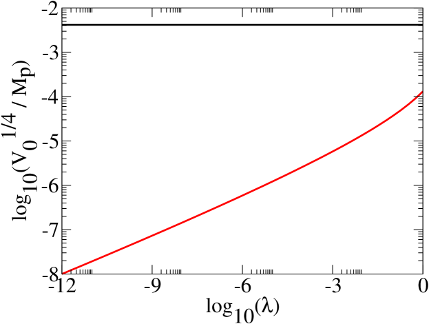
Figure 1: The parameter space in tachyonic preheating allowed by the WMAP data for single field inflation (below the red curve). Black horizontal line is the usual limit $V_{0}^{1/4}=10^{16}$ GeV coming from the COBE normalization.

When obtaining the result above we have assumed that the first order metric perturbations is roughly given by the constant value determined by the inflationary epoch. Let us investigate the other limit when the first order metric fluctuations also obtain an exponentially growing solution by virtue of the tachyon excitations. To check this possibility, let us assume that the exponential solution actually dominates over the constant one. Following the second order analysis and assuming that the main contribution to the second order perturbation arises from the tachyonic instability, we obtain from Eq. (10)

$$\ddot{\phi}^{(2)}-2A\,\dot{\phi}^{(2)}=-\kappa^{2}\left[2(\delta^{(1)}\dot{\chi})^{2}+8\dot{\chi}_{0}^{2}(\phi^{(1)})^{2}-V_{,\chi\chi}(\delta^{(1)}\chi)^{2}-8\dot{\chi}_{0}\phi^{(1)}\delta^{(1)}\dot{\chi}\right],$$ (29)

where $V_{,\chi\chi}=-m^{2}+3\lambda\chi^{2}$ and where $\delta^{(1)}\chi$ can be solved through the Einstein constraint [9] $\delta^{(1)}\chi=\frac{2}{\kappa^{2}\dot{\chi}_{0}}\left(\dot{\phi}^{(1)}+H\phi^{(1)}\right)$.

For the tachyonic region $3\lambda\chi^{2}<m^{2}$ so that we can take $V_{,\chi\chi}\sim-m^{2}$. Now $\phi^{(2)}$ contains the homogeneous solution $\sim\exp(2At)$ together with a source part $\sim\exp(4At)$ . After a while the source part dominates and we obtain the result

$$f_{NL}^{\phi}=\frac{\phi^{(2)}}{(\phi^{(1)})^{2}}=\left|8-\frac{2m^{2}}{\kappa^{2}\dot{\chi}_{0}^{2}}-\frac{4\ddot{\chi}_{0}^{2}}{\kappa^{2}\dot{\chi}_{0}^{4}}-\frac{\kappa^{2}\dot{\chi}_{0}^{4}}{\ddot{\chi}_{0}^{2}}\right|\,.$$ (30)

The tachyonic growth persists until $\chi\sim m/(2\sqrt{\lambda})$, for a time span $t_{\ast}\sim(1/2m)\ln(\pi^{2}/\lambda)$  [16]. With these approximations, writing $V_{0}=m^{4}/(4\lambda)$, we obtain

$$f_{NL}^{\phi}\approx 8-8\sqrt{\frac{\lambda M_{P}^{4}}{V_{0}}}-\frac{1}{2}\sqrt{\frac{V_{0}}{\lambda M_{P}^{4}}}-\sqrt{\frac{\lambda M_{P}^{4}}{V_{0}}}{\rm ln}^{2}\left(\frac{\pi^{2}}{\lambda}\right)\,.$$ (31)

If we assume COBE normalization $V_{0}^{1/4}\leq 10^{16}$ GeV, the minimum of $V_{0}$ is given by the conditions ${V_{0}^{1/4}}/{M_{P}}=\lambda^{1/4}\sqrt{8-f_{NL}^{\phi}}$ and $\lambda=\pi^{2}\exp(-\sqrt{(8-f_{NL}^{\phi})^{2}/2-8})$. These imply the limit $f_{NL}^{\phi}<-37$ regardless of the value of $\lambda$, well within the observational capabilities of WMAP.

Many string-motivated inflationary models could thus be constrained by the present and future limits on non-Gaussianity. An example would be inflation first driven by brane-anti-brane interaction and then coming to an end when the tachyonic instability is triggered [20]. Should we take the tachyon coupling to be very small $\lambda\sim 10^{-12}$, as constrained by the amplitude of the CMB scalar fluctuations [21], we immediately obtain from Eq. (28) that $V_{0}^{1/4}/M_{P}\leq 10^{-7}$ in order to comply with the current WMAP limit on non-Gaussianity. Such considerations imply very interesting constraints on the scale of the tachyonic instability and on the tachyon self coupling in brane-anti-brane driven inflation.

In obtaining our limits we have made some approximations. In particular, we assumed that the VEV of $\sigma$ field is vanishing in the instant preheating case and in tachyonic preheating we assumed that the inflaton VEV is vanishing after the end of inflation. These assumptions make our analysis simple and provide a handle on the non-Gaussianity parameter.

We are thankful to Robert Brandenberger, Cliff Burgess, Andrew Liddle, David Lyth, Licia Verde and Filippo Vernizzi for discussions. A.V. is supported by the Magnus Ehrnrooth Foundation. A.V. thanks NORDITA and NBI for their kind hospitality during the course of this work. K.E. is supported in part by the Academy of Finland grant no. 75065.

References

- [1] J. H. Traschen and R. H. Brandenberger, Phys. Rev. D 42, 2491 (1990).
- [2] L. Kofman, A. D. Linde and A. A. Starobinsky, Phys. Rev. Lett. 76, 1011 (1996) [arXiv:hep-th/9510119]; Y. Shtanov, J. H. Traschen and R. H. Brandenberger, Phys. Rev. D 51, 5438 (1995) [arXiv:hep-ph/9407247]; D. Boyanovsky, H. J. de Vega and R. Holman, arXiv:hep-ph/9701304, and refs. therein.
- [3] L. Kofman, A. D. Linde and A. A. Starobinsky, Phys. Rev. D 56, 3258 (1997) [arXiv:hep-ph/9704452].
- [4] D. Cormier, K. Heitmann and A. Mazumdar, Phys. Rev. D 65, 083521 (2002) [arXiv:hep-ph/0105236].
- [5] P. Jaikumar and A. Mazumdar, Nucl. Phys. B 683, 264 (2004) [arXiv:hep-ph/0212265]; K. Enqvist and J. Högdahl, arXiv:hep-ph/0405299.
- [6] B. A. Bassett, D. I. Kaiser and R. Maartens, Phys. Lett. B 455, 84 (1999) [arXiv:hep-ph/9808404]; B. A. Bassett, F. Tamburini, D. I. Kaiser and R. Maartens, Nucl. Phys. B 561, 188 (1999) [arXiv:hep-ph/9901319]; K. Jedamzik and G. Sigl, Phys. Rev. D 61, 023519 (2000) [arXiv:hep-ph/9906287]; F. Finelli and R. H. Brandenberger, Phys. Rev. Lett. 82, 1362 (1999) [arXiv:hep-ph/9809490]; F. Finelli and R. H. Brandenberger, Phys. Rev. D 62, 083502 (2000) [arXiv:hep-ph/0003172]; A. R. Liddle, D. H. Lyth, K. A. Malik and D. Wands, Phys. Rev. D 61, 103509 (2000) [arXiv:hep-ph/9912473].
- [7] M. Parry and R. Easther, Phys. Rev. D 59, 061301 (1999) [arXiv:hep-ph/9809574]; R. Easther and M. Parry, Phys. Rev. D 62, 103503 (2000) [arXiv:hep-ph/9910441]; F. Finelli and S. Khlebnikov, Phys. Lett. B 504 (2001) 309 [arXiv:hep-ph/0009093]; F. Finelli and S. Khlebnikov, Phys. Rev. D 65 (2002) 043505 [arXiv:hep-ph/0107143].
- [8] V. F. Mukhanov, H. A. Feldman and R. H. Brandenberger, Phys. Rept. 215, 203 (1992).
- [9] N. Bartolo, E. Komatsu, S. Matarrese and A. Riotto, Phys. Rept. 402 (2004) 103 [arXiv:astro-ph/0406398].
- [10] K. Enqvist, A. Jokinen, A. Mazumdar, T. Multamäki and A. Väihkönen, arXiv:astro-ph/0411394.
- [11] V. Acquaviva, N. Bartolo, S. Matarrese and A. Riotto, Nucl. Phys. B 667 (2003) 119 [arXiv:astro-ph/0209156].
- [12] K. Enqvist and A. Väihkönen, JCAP 0409, 006 (2004) [arXiv:hep-ph/0405103].
- [13] K. Enqvist, S. Kasuya and A. Mazumdar, Phys. Rev. Lett. 90, 091302 (2003) [arXiv:hep-ph/0211147]; K. Enqvist, A. Jokinen, S. Kasuya and A. Mazumdar, Phys. Rev. D 68, 103507 (2003) [arXiv:hep-ph/0303165]; K. Enqvist, S. Kasuya and A. Mazumdar, Phys. Rev. Lett. 93, 061301 (2004) [arXiv:hep-ph/0311224]; K. Enqvist, A. Mazumdar and A. Perez-Lorenzana, arXiv:hep-th/0403044.
- [14] N. Bartolo, S. Matarrese and A. Riotto, JHEP 0404, 006 (2004) [arXiv:astro-ph/0308088].
- [15] G. N. Felder, L. Kofman and A. D. Linde, Phys. Rev. D 59, 123523 (1999) [arXiv:hep-ph/9812289].
- [16] G. N. Felder, J. Garcia-Bellido, P. B. Greene, L. Kofman, A. D. Linde and I. Tkachev, Phys. Rev. Lett. 87, 011601 (2001) [arXiv:hep-ph/0012142].
- [17] K. Enqvist and A. Mazumdar, Phys. Rept. 380, 99 (2003) [arXiv:hep-ph/0209244].
- [18] D. Babich and M. Zaldarriaga, Phys. Rev. D 70 (2004) 083005 [arXiv:astro-ph/0408455].
- [19] E. Komatsu et al., Astrophys. J. Suppl. 148 (2003) 119 [arXiv:astro-ph/0302223].
- [20] C. P. Burgess, M. Majumdar, D. Nolte, F. Quevedo, G. Rajesh and R. J. Zhang, JHEP 0107, 047 (2001) [arXiv:hep-th/0105204]; A. Mazumdar, S. Panda and A. Perez-Lorenzana, Nucl. Phys. B 614, 101 (2001) [arXiv:hep-ph/0107058].
- [21] H. V. Peiris et al., Astrophys. J. Suppl. 148 (2003) 213 [arXiv:astro-ph/0302225].