Next-to-leading order QCD predictions for $A^{0}Z^{0}$ associated production at the CERN Large Hadron Collider

Abstract

We present the calculations of the complete next-to-leading order (NLO) QCD corrections (including supersymmetric QCD) to the inclusive total cross sections of the associated production processes $pp\rightarrow A^{0}Z^{0}+X$ in the Minimal Supersymmetric Standard Model at the CERN Large Hadron Collider. Both the dimensional regularization scheme and the dimensional reduction scheme are used to organize the calculations which yield the same NLO rates. The NLO correction can either enhance or reduce the total cross sections, but it generally efficiently reduces the dependence of the total cross sections on the renormalization/factorization scale. We also examine the uncertainty of the total cross sections due to the parton distribution function uncertainties.

I Introduction

The search for one or more Higgs bosons is the central task of the CERN Large Hadron Collider (LHC), with $\sqrt{S}=14$ TeV and a luminosity of 100 ${\rm fb^{-1}}$ per year. In the Standard Model (SM), the Higgs boson mass is a free parameter with an upper bound of $m_{H}\leq 600$ — 800 GeV massh . Beyond the SM, the Minimal Supersymmetric Standard Model (MSSM), whose Higgs sector is a special case of the Two Higgs Doublet Model (2HDM) mssm , is of particular theoretical interest, and contains five physical Higgs bosons: two neutral CP-even bosons $h^{0}$ and $H^{0}$, one neutral CP-odd boson $A^{0}$, and two charged bosons $H^{\pm}$. The $h^{0}$ is the lightest, with a mass $m_{h^{0}}\leq 140$  GeV when including the radiative corrections massh0 , and is a SM-like Higgs boson especially in the decoupling region ($m_{A^{0}}\gg m_{Z^{0}}$). The other four are non-SM-like ones, and the discovery of them may give the direct evidence of the MSSM. It has been shown in detect ; LHCHiggs that the $h^{0}$ boson of MSSM cannot escape detection at the CERN Large Hadron Collider (LHC) and that more than one neutral Higgs particle can be found in large area of the supersymmetry (SUSY) parameter space

At the LHC, the neutral Higgs bosons can be produced through following mechanisms: gluon fusion $gg\rightarrow\phi$ gg2h ; gg2hnlo ; gg2hnnlo ; gg2hresum , weak boson fusion $qq\rightarrow qqV^{*}V^{*}\rightarrow qqh^{0}/qqH^{0}$ vv2h , associated production with weak bosons wzh ; v2vh ; v22 , associated production with a heavy quark-antiquark pair $gg,q\bar{q}\rightarrow t\bar{t}\phi/b\bar{b}\phi$ ttbbh and pairs production hpair . Studying the associated production process of a neutral Higgs boson and a vector boson at future hadron colliders may be an interesting way in searching for neutral Higgs bosons, since the total cross section may be large and also the leptonic decay of the vector boson can be used as a spectacular event trigger. In the SM, the process $q\bar{q}^{(\prime)}\rightarrow W/Z^{0}h^{0}_{SM}$ has been studied both at the leading order (LO) wzh and the next-to-leading order (NLO) v22 ; wzhnlo in QCD. In the 2DHM and MSSM, the associated production of $h^{0}(H^{0})Z^{0}$ and $A^{0}Z^{0}$ has been studied only at tree level for Drell-Yan process and at one-loop level for gluon fusion in hHZLO and AZLO ; KaoAZLO ; Kao , respectively.

It was shown in Ref. AZLO that the $A^{0}Z^{0}$ associated production rate at the LHC strongly depends on the SUSY parameters $\tan{\beta}$ (the ratio of two vacuum expectation values) and $m_{A}$ (the mass of $A^{0}$). The total cross section increases with increment of $\tan{\beta}$, and decreases with increment of $m_{A}$. In this paper, we present the complete NLO QCD, including supersymmetric QCD, calculation for the cross section of the associated production of $A^{0}Z^{0}$ through $b\bar{b}$ annihilation process at the LHC. For simplicity, in our calculation, we neglect the bottom quark mass except in the Yukawa couplings. Such approximations are valid in all diagrams, in which the bottom quark appears as an initial state parton, according to the simplified Aivazis-Collins-Olness-Tung (ACOT) scheme acot . To regularize the ultraviolet (UV), soft and collinear divergences, two regularization schemes are used in our calculations for cross check, i.e. the dimensional regularization (DREG) scheme DREG (with naive $\gamma_{5}$ scheme gamma5 ) and the dimensional reduction (DRED) scheme DRED , and their results are compared.

The arrangement of this paper is as follows. In Sect. II, we show the LO results and define the notations. In Sect. III, we present the details of the calculations of both the virtual and real parts of the NLO QCD corrections, and compare the results in DREG with those in DRED. In Sect. IV, by a detailed numerical analysis, we present the predictions for the inclusive and differential cross sections of the $A^{0}Z^{0}$ associated production at the LHC. Sec. V contains a brief conclusion. For completeness, the relevant Feynman rules are collected in Appendix A, and the lengthy analytic expressions of the result of our calculation are summarized in Appendices B and C.

II Leading order calculations

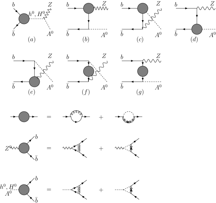
The related Feynman diagrams which contribute to the LO amplitude of the partonic process $b(p_{1})\bar{b}(p_{2})\rightarrow Z^{0}(p_{3})A^{0}(p_{4})$ are shown in Fig. 1. The LO amplitude in $n=4-2\epsilon$ dimensions is

$$M^{B}=\delta_{i_{1}i_{2}}\mu_{r}^{4-n}[M^{(s)}_{0}+M^{(t)}_{0}+M^{(u)}_{0}]$$

with

$$M^{(s)}_{0}=2im_{b}\bigg{(}\frac{A_{1}F_{1}}{s-m^{2}_{h^{0}}}+\frac{A_{2}F_{2}}{s-m^{2}_{H^{0}}}\bigg{)}\overline{v}(p_{2})u(p_{1})p_{4}.\varepsilon_{\rho}(p_{3})\,,$$

$$M^{(t)}_{0}=\frac{im_{b}A_{3}}{t}\overline{v}(p_{2})\gamma^{5}(\not{\!p}_{1}-\not{\!p}_{3})\not{\!\varepsilon}(p_{3})(C_{V}+C_{A}\gamma^{5})u(p_{1})\,,$$

$$M^{(u)}_{0}=\frac{im_{b}A_{3}}{u}\overline{v}(p_{2})\not{\!\varepsilon}(p_{3})(C_{V}+C_{A}\gamma^{5})(\not{\!p}_{1}-\not{\!p}_{4})\gamma^{5}u(p_{1}),$$

where $\delta_{i_{1}i_{2}}$ is the color tensor ($i_{1},i_{2}$ are color indices for the initial state quarks), $\mu_{r}$ is a mass parameter introduced to keep the couplings dimensionless, $s,t$ and $u$ are Mandelstam variables, which are defined as

$$s=(p_{1}+p_{2})^{2},\qquad t=(p_{1}-p_{3})^{2},\qquad u=(p_{2}-p_{3})^{2},$$

$A_{i=1,2,3}$, $F_{i=1,2}$ and $C_{V,A}$ denote the coefficients appearing in the relevant $h^{0}(H^{0},A^{0})b\bar{b}$, $h^{0}(H^{0})Z^{0}A^{0}$ and $Z^{0}b\bar{b}$ couplings, respectively, and their explicit expressions are given in Appendix A.

In order to simplify the expressions, we further introduce the following Mandelstam variables:

$$t^{\prime}=t-m_{Z^{0}}^{2},\ \ \ u^{\prime}=u-m_{Z^{0}}^{2}.$$ (1)

After the $n$-dimensional phase space integration, the LO partonic differential cross sections are given by

$$\frac{d^{2}\hat{\sigma}^{B}}{dt^{\prime}du^{\prime}}=\frac{\pi S_{\epsilon}}{s^{2}\Gamma(1-\epsilon)}\bigg{(}\frac{t^{\prime}u^{\prime}-sm_{Z^{0}}^{2}}{\mu_{r}^{2}s}\bigg{)}^{-\epsilon}\Theta(t^{\prime}u^{\prime}-sm_{Z^{0}}^{2})\Theta[s-(m_{Z^{0}}+m_{A^{0}})^{2}]$$

$$\hskip 51.21504pt\times\delta(s+t+u-m_{Z^{0}}^{2}-m_{A^{0}}^{2})\overline{\sum}|M^{B}|^{2}$$ (2)

with

$$\overline{\sum}{|M^{B}|}^{2}=\frac{m^{2}_{b}}{6}\Bigg{\{}\bigg{[}4m^{2}_{A^{0}}s-\frac{(s-m_{Z^{0}}^{2}-m_{A^{0}}^{2})^{2}s}{m^{2}_{Z^{0}}}\bigg{]}\bigg{(}\frac{A_{1}F_{1}}{s-m^{2}_{h^{0}}}+\frac{A_{2}F_{2}}{s-m^{2}_{H^{0}}}\bigg{)}^{2}$$

$$\hskip 56.9055pt+A_{3}^{2}(|C_{V}|^{2}+|C_{A}|^{2})\frac{2m^{2}_{Z^{0}}(1-\epsilon)(tu-m^{2}_{Z^{0}}m^{2}_{A^{0}})+st^{2}}{m^{2}_{Z^{0}}t^{2}}$$

$$\hskip 56.9055pt+A_{3}^{2}(|C_{V}|^{2}+|C_{A}|^{2})\frac{2m^{2}_{Z^{0}}(1-\epsilon)(tu-m^{2}_{Z^{0}}m^{2}_{A^{0}})+su^{2}}{m^{2}_{Z^{0}}u^{2}}$$

$$\hskip 56.9055pt+\frac{4A_{3}C_{A}s(t+u)(tu-m^{2}_{Z^{0}}m^{2}_{A^{0}})}{tum^{2}_{Z^{0}}}\bigg{[}\frac{A_{1}F_{1}}{(s-m^{2}_{h^{0}})}+\frac{A_{2}F_{2}}{(s-m^{2}_{H^{0}})}\bigg{]}$$

$$\hskip 56.9055pt+2A_{3}^{2}(|C_{V}|^{2}-|C_{A}|^{2})\frac{2(1-\epsilon)m^{2}_{Z^{0}}(tu-m^{2}_{Z^{0}}m^{2}_{A^{0}})+s(2m^{2}_{Z^{0}}m^{2}_{A^{0}}-tu)}{m^{2}_{Z^{0}}tu}\Bigg{\}},$$ (3)

where $S_{\epsilon}=(4\pi)^{-2+\epsilon}$ and the $\Theta$ function is the Heaviside step function. $\overline{\sum}{|M^{B}|}^{2}$ is the LO squared matrix element of $b(x_{1}p_{1})\bar{b}(x_{2}p_{2})\rightarrow Z^{0}(p_{3})A^{0}(p_{4})$, in which the colors and spins of the outgoing particles have been summed, and the colors and spins of the incoming ones have been averaged over.

The LO total cross section at the LHC is obtained by convoluting the partonic cross section with the parton distribution functions (PDFs) $G_{b,\bar{b}/p}$ in the proton:

$$\sigma^{B}=\int dx_{1}dx_{2}[G_{b/p}(x_{1},\mu_{f})G_{\bar{b}/p}(x_{2},\mu_{f})+(x_{1}\leftrightarrow x_{2})]\hat{\sigma}^{B},$$ (4)

where $\mu_{f}$ is the factorization scale and $\hat{\sigma}^{B}$ is the Born level constituent cross section of $b(x_{1}p_{1})\bar{b}(x_{2}p_{2})\rightarrow Z^{0}(p_{3})A^{0}(p_{4})$. Obviously, the above LO results in the DREG scheme are equal to the ones in the DRED scheme since the LO calculations are finite and free of any singularity.

III Next-to-Leading order calculations

The NLO contributions to the associated production of $A^{0}$ and $Z^{0}$ can be separated into the virtual corrections arising from loop diagrams of colored particles and the real corrections arising from the radiation of a real gluon or a massless (anti)quark. For both the virtual and real corrections, we will first present the results in the DREG scheme, and then compare them with the ones obtained in the DRED scheme.

III.1 Virtual corrections

The virtual corrections to $b\bar{b}\rightarrow A^{0}Z^{0}$ arise from the Feynman diagrams shown in Fig. 2 and Fig. 3. They consist of self-energy, vertex and box diagrams, which represent the SM QCD corrections, arising from quarks and gluons, and supersymmetric QCD corrections, arising from squarks and gluinos. We carried out the calculation in t’Hooft-Feynman gauge and used the dimensional regularization in $n=4-2\epsilon$ dimensions to regularize the ultraviolet (UV), soft and collinear divergences in the virtual loop corrections. In order to remove the UV divergences, we renormalize the bottom quark masses in the Yukawa couplings and the wave function of bottom quark, adopting the on-shell renormalization scheme onmass .

Denoting $m_{b0}$ and $\psi_{b0}$ as the bare bottom quark mass and the bare wave function, respectively, the relevant renormalization constants $\delta m_{b},\delta Z_{bL}$ and $\delta Z_{bR}$ are then defined as

$$m_{b0}=m_{b}+\delta m_{b},$$ (5)

$$\psi_{b0}=(1+\delta Z_{bL})^{\frac{1}{2}}\psi_{bL}+(1+\delta Z_{bR})^{\frac{1}{2}}\psi_{bR}.$$ (6)

After calculating the self-energy diagrams in Fig. 2, we obtain the explicit expressions of all the renormalization constants as follows:

$$\frac{\delta m_{b}}{m_{b}}=-\frac{\alpha_{s}}{4\pi}C_{F}\bigg{\{}3B_{0}(m_{b}^{2},0,m_{b}^{2})-2$$

$$\hskip 34.14322pt+\sum_{i=1}^{2}\bigg{[}B_{1}-\frac{m_{\tilde{g}}}{m_{b}}\sin 2\theta_{\tilde{b}}(-1)^{i}B_{0}\bigg{]}(m_{b}^{2},m_{\tilde{g}}^{2},m_{\tilde{b}_{i}}^{2})\bigg{\}},$$

$$\delta Z_{bL}=-\frac{\alpha_{s}}{2\pi}C_{F}\sum_{i=1}^{2}(R^{\tilde{b}}_{i1})^{2}(B_{0}+B_{1})(0,m_{\tilde{b}_{i}}^{2},m_{\tilde{g}}^{2}),$$

$$\delta Z_{bR}=-\frac{\alpha_{s}}{2\pi}C_{F}\sum_{i=1}^{2}(R^{\tilde{b}}_{i2})^{2}(B_{0}+B_{1})(0,m_{\tilde{b}_{i}}^{2},m_{\tilde{g}}^{2}),$$

where $C_{F}=\frac{4}{3}$, $B_{0},B_{1}$ are the scalar two-point integrals denner , $m_{\tilde{b}_{1,2}}$ are the sbottom masses, $m_{\tilde{g}}$ is the gluino mass, and $R^{\tilde{b}}$ is a $2\times 2$ matrix shown as below, which is defined to transform the sbottom current eigenstates to the mass eigenstates rotMa :

$$\left(\begin{array}[]{c}\tilde{b}_{1}\\ \tilde{b}_{2}\end{array}\right)=R^{\tilde{b}}\left(\begin{array}[]{c}\tilde{b}_{L}\\ \tilde{b}_{R}\end{array}\right),\ \ \ \ \ R^{\tilde{b}}=\left(\begin{array}[]{cc}\cos\theta_{\tilde{b}}&\sin\theta_{\tilde{b}}\\ -\sin\theta_{\tilde{b}}&\cos\theta_{\tilde{b}}\end{array}\right)$$ (7)

with $0\leq\theta_{\tilde{b}}<\pi$, by convention. Correspondingly, the mass eigenvalues $m_{\tilde{b}_{1}}$ and $m_{\tilde{b}_{2}}$ (with $m_{\tilde{b}_{1}}\leq m_{\tilde{b}_{2}}$) are given by

$$\left(\begin{array}[]{cc}m_{\tilde{b}_{1}}^{2}&0\\ 0&m_{\tilde{b}_{2}}^{2}\end{array}\right)=R^{\tilde{b}}M_{\tilde{b}}^{2}(R^{\tilde{b}})^{\dagger},\ \ \ \ \ M_{\tilde{b}}^{2}=\left(\begin{array}[]{cc}m_{\tilde{b}_{L}}^{2}&a_{b}m_{b}\\ a_{b}m_{b}&m_{\tilde{b}_{R}}^{2}\end{array}\right)$$ (12)

with

$$m^{2}_{\tilde{b}_{L}} = M^{2}_{\tilde{Q}}+m_{b}^{2}+m_{Z}^{2}\cos 2\beta(I_{3L}^{b}-e_{b}\sin^{2}\theta_{W}),$$ (13)

$$m^{2}_{\tilde{b}_{R}} = M^{2}_{\tilde{D}}+m_{b}^{2}+m_{Z}^{2}\cos 2\beta e_{b}\sin^{2}\theta_{W},$$ (14)

$$a_{b} = A_{b}-\mu\tan\beta.$$ (15)

Here, $M_{\tilde{b}}^{2}$ is the sbottom mass matrix. $M_{\tilde{Q},\tilde{D}}$ and $A_{b}$ are soft SUSY breaking parameters and $\mu$ is the higgsino mass parameter . $I_{3L}^{b}$ and $e_{b}$ are the third component of the weak isospin (i.e. $-1/2$) and the electric charge of the bottom quark $b$ (i.e. $-1/3$), respectively.

The renormalized virtual amplitudes can be written as

$$M^{V}=M^{unren}+M^{con}.$$ (16)

Here, $M^{unren}$ contains the radiative corrections from the one-loop self-energy, vertex and box diagrams, as shown in Fig. 2, and $M^{con}$ is the corresponding counterterm. Moreover, $M^{unren}$ can be separated into two parts:

$$M^{unren}=\sum_{\alpha=a}^{g}M^{\alpha}+\sum_{\beta=a}^{d}M^{{\rm box}(\beta)},$$ (17)

where $\alpha$ and $\beta$ denote the corresponding diagram indexes in Fig. 2 and Fig. 3, respectively. They can be further expressed as

$$M^{\alpha}=\sum_{l=1}^{12}f_{l}^{\alpha}M_{l},$$ (18)

$$M^{box(\beta)}=\sum_{l=1}^{12}f_{l}^{box(\beta)}M_{l},$$ (19)

$$M^{unren}=\sum_{l=1}^{12}f_{l}^{unren}M_{l},\hskip 28.45274pt(f_{l}^{unren}=f_{l}^{\alpha}+f_{l}^{box(\beta)})\,,$$ (20)

where $f_{l}^{\alpha}$ and $f_{l}^{box(\beta)}$ are the form factors, which are given explicitly in Appendix B, and the $M_{l}$ are the standard matrix elements defined as

$$M_{1(2)}=\bar{v}(p_{2})u(p_{1})p_{1(2)}.\epsilon(p_{3}),$$

$$M_{3(4)}=\bar{v}(p_{2})P_{R}u(p_{1})p_{1(2)}.\epsilon(p_{3}),$$

$$M_{5}=\bar{v}(p_{2})\not{\!p}_{3}\not{\!\epsilon}(p_{3})u(p_{1}),$$

$$M_{6}=\bar{v}(p_{2})\not{\!p}_{3}\not{\!\epsilon}(p_{3})P_{R}u(p_{1}),$$

$$M_{7(8)}=\bar{v}(p_{2})\not{\!p}_{3}P_{R}u(p_{1})p_{1(2)}.\epsilon(p_{3}),$$

$$M_{9}=\bar{v}(p_{2})\not{\!\epsilon}(p_{3})u(p_{1}),$$

$$M_{10}=\bar{v}(p_{2})\not{\!\epsilon}(p_{3})P_{R}u(p_{1}),$$

$$M_{11(12)}=\bar{v}(p_{2})\not{\!p}_{3}u(p_{1})p_{1(2)}.\epsilon(p_{3}).$$ (21)

The counterterm contribution $M^{con}$ is separated into $M^{con(s)}$, $M^{con(t)}$ and $M^{con(u)}$, i.e. the counterterms for s, t and u channels, respectively, which are given by

$$M^{con}=M^{con(s)}+M^{con(t)}+M^{con(u)},$$

$$M^{con(s)}=2i\bigg{(}\frac{A_{1}F_{1}}{s-m^{2}_{h^{0}}}+\frac{A_{2}F_{2}}{s-m^{2}_{H^{0}}}\bigg{)}\bigg{[}\delta m_{b}+\frac{m_{b}}{2}(\delta Z_{bL}+\delta Z_{bR})\bigg{]}(M_{1}+M_{2})\,,$$

$$M^{con(t)}=\frac{-iA_{3}}{t}\bigg{[}\delta m_{b}+\frac{m_{b}}{2}(\delta Z_{bL}+\delta Z_{bR})\bigg{]}[2(C_{V}-C_{A})M_{1}-4C_{V}M_{3}$$

$$\hskip 122.34692pt-(C_{V}-C_{A})M_{5}+2C_{V}M_{6}]\,,$$

$$M^{con(u)}=\frac{iA_{3}}{u}\bigg{[}\delta m_{b}+\frac{m_{b}}{2}(\delta Z_{bL}+\delta Z_{bR})\bigg{]}[2(C_{V}+C_{A})M_{2}-4C_{V}M_{4}$$

$$\hskip 122.34692pt+(C_{V}+C_{A})M_{5}-2C_{V}M_{6}]\,.$$

The ${\cal O}(\alpha_{s})$ virtual corrections to the differential cross section can be expressed as

$$\frac{d^{2}\hat{\sigma}^{V}}{dt^{\prime}du^{\prime}}=\frac{\pi S_{\epsilon}}{s^{2}\Gamma(1-\epsilon)}\bigg{(}\frac{t^{\prime}u^{\prime}-sm_{Z^{0}}^{2}}{\mu_{r}^{2}s}\bigg{)}^{-\epsilon}\Theta(t^{\prime}u^{\prime}-sm_{Z^{0}}^{2})\Theta[s-(m_{Z^{0}}+m_{A^{0}})^{2}]$$

$$\hskip 51.21504pt\times\delta(s+t+u-m_{A^{0}}^{2}-m_{Z^{0}}^{2})\ 2\ {\rm Re}\bigg{[}\overline{\sum}{(M^{V}M^{B\ast})}\bigg{]},$$ (22)

where the renormalized amplitude $M^{V}$ is UV finite, but it still contains the infrared (IR) divergences:

$$M^{V}|_{IR}=\frac{\alpha_{s}}{2\pi}\frac{\Gamma(1-\epsilon)}{\Gamma(1-2\epsilon)}\bigg{(}\frac{4\pi\mu_{r}^{2}}{s}\bigg{)}^{\epsilon}\bigg{(}\frac{A_{2}^{V}}{\epsilon^{2}}+\frac{A_{1}^{V}}{\epsilon}\bigg{)}M^{B},$$ (23)

where

$$A_{2}^{V}=-C_{F},\qquad A_{1}^{V}=-\frac{3}{2}C_{F}.$$ (24)

Here, the infrared divergences include the soft divergences and the collinear divergences. The soft divergences are cancelled after adding the real emission corrections, and the remaining collinear divergences can be absorbed into the redefinition of PDF altarelli , which will be discussed in the following subsections. Note that the coefficients $A_{2}^{V}$ and $A_{1}^{V}$ of the infrared divergence terms are constants, similar to the Drell-Yan type processes. Needless to say that the SUSY QCD corrections do not generate infrared divergences, for squarks and gluinos are massive particles.

In the above calculation, we have adopted the naive $\gamma_{5}$ prescription in the DREG scheme to calculate the $A^{0}Z^{0}$ associated production rate. To cross check the above calculation, we shall also adopt the DRED scheme to carefully treat the $\gamma_{5}$ factor in the amplitude calculation. We shall show that the total inclusive rate is independent of the regularization scheme, though the individual contributions, from either virtual or real emission corrections, can be scheme-dependent.

In the DRED scheme, $\delta Z_{bL}$ and $\delta Z_{bR}$ remain unchanged, however, $\delta m_{b}$ is different, and

$$\bigg{(}\frac{\delta m_{b}}{m_{b}}\bigg{)}_{DREG}-\bigg{(}\frac{\delta m_{b}}{m_{b}}\bigg{)}_{DRED}=\frac{\alpha_{s}}{4\pi}C_{F}.$$ (25)

Similarly, the form factors are found to be different, and

$${f_{i}^{unren}}_{DREG}-{f_{i}^{unren}}_{DRED}=-\frac{\alpha_{s}}{2\pi}C_{F}\,,\hskip 17.07182pt{\rm for}\quad i=1,2...6,$$ (26)

$${f_{i}^{unren}}_{DREG}-{f_{i}^{unren}}_{DRED}=0\,,\hskip 17.07182pt{\rm for}\quad i=7,8...12.$$ (27)

Thus, it is easy to obtain the following relations from the above results:

$${M^{V}}_{DREG}-{M^{V}}_{DRED}=-\frac{\alpha_{s}}{4\pi}C_{F}M^{B},$$ (28)

$${\sigma^{V}}_{DREG}-{\sigma^{V}}_{DRED}=-\frac{\alpha_{s}}{2\pi}C_{F}\sigma^{B}+{\cal O}(\alpha^{2}_{s}).$$ (29)

III.2 Real gluon emission

The Feynman diagrams for the real gluon emission process $b(p_{1})\bar{b}(p_{2})\rightarrow Z^{0}(p_{3})A^{0}(p_{4})+g(p_{5})$ are shown in Fig. 4.

The phase space integration for the real gluon emission will produce infrared singularities, which can be either soft or collinear and can be conveniently isolated by slicing the phase space into different regions defined by suitable cut-offs. In this paper, we use the two-cutoff phase space slicing method cutoff which introduces two small cut-offs to decompose the three-body phase space into three regions.

First, the phase space can be separated into two regions by an arbitrary small soft cut-off $\delta_{s}$, according to whether the energy ($E_{5}$) of the emitted gluon is soft, i.e. $E_{5}\leq\delta_{s}\sqrt{s}/2$, or hard, i.e. $E_{5}>\delta_{s}\sqrt{s}/2$. Correspondingly, the partonic real cross section can be written as

$$\hat{\sigma}^{R}=\hat{\sigma}^{S}+\hat{\sigma}^{H},$$ (30)

where $\hat{\sigma}^{S}$ and $\hat{\sigma}^{H}$ are the contributions from the soft and hard regions, respectively. $\hat{\sigma}^{S}$ contains all the soft divergences, which can be explicitly obtained after analytically integrating over the phase space of the emitted soft gluon. Second, in order to isolate the remaining collinear divergences from $\hat{\sigma}^{H}$, we should introduce another arbitrary small cut-off, called collinear cut-off $\delta_{c}$, to further split the hard gluon phase space into two regions, according to whether the Mandelstam variables satisfy the collinear condition $-\delta_{c}s<u_{1,2}\equiv(p_{1,2}-p_{5})^{2}<0$ or not. Thus, we have

$$\hat{\sigma}^{H}=\hat{\sigma}^{HC}+\hat{\sigma}^{\overline{HC}},$$ (31)

where the hard collinear part $\hat{\sigma}^{HC}$ contains the collinear divergences, which can be explicitly obtained after analytically integrating over the phase space of the emitted collinear gluon. The hard non-collinear part $\hat{\sigma}^{\overline{HC}}$ is finite and can be numerically computed using standard Monte-Carlo integration techniques Monte , and can be written in the form:

$$d\hat{\sigma}^{\overline{HC}}=\frac{1}{2s}\overline{\sum}{|M^{b\bar{b}}|}^{2}d\overline{\Gamma}_{3}.$$ (32)

Here, $d\overline{\Gamma}_{3}$ is the hard non-collinear region of the three-body phase space.

In the next two subsections, we will discuss in detail the soft and hard collinear gluon emission.

III.2.1 Soft gluon emission

In the soft limit, i.e. when the energy of the emitted gluon is small, with $E_{5}\leq\delta_{s}\sqrt{s}/2$, the matrix element squared $\overline{\sum}{|M^{R}|}^{2}$ for the process $b(p_{1})\bar{b}(p_{2})\rightarrow Z^{0}(p_{3})A^{0}(p_{4})g(p_{5})$ can be simply factorized into the Born matrix element squared times an eikonal factor $\Phi_{eik}$:

$$\overline{\sum}{|M^{R}(b\bar{b}\rightarrow A^{0}Z^{0}+g)|}^{2}\stackrel{{\scriptstyle soft}}{{\rightarrow}}(4\pi\alpha_{s}\mu_{r}^{2\epsilon})\overline{\sum}{|M^{B}|}^{2}\Phi_{eik},$$ (33)

where the eikonal factor $\Phi_{eik}$ is given by

$$\Phi_{eik}=C_{F}\frac{s}{(p_{1}\cdot p_{5})(p_{2}\cdot p_{5})}.$$ (34)

Moreover, the phase space in the soft limit can also be factorized as

$$d\Gamma_{3}(b\bar{b}\rightarrow A^{0}Z^{0}+g)\stackrel{{\scriptstyle soft}}{{\rightarrow}}d\Gamma_{2}(b\bar{b}\rightarrow A^{0}Z^{0})dS,$$ (35)

where $dS$ is the integration over the phase space of the soft gluon, which is given by cutoff

$$dS=\frac{1}{2(2\pi)^{3-2\epsilon}}\int_{0}^{\delta_{s}\sqrt{s}/2}dE_{5}E_{5}^{1-2\epsilon}d\Omega_{2-2\epsilon}.$$ (36)

Hence, the parton level cross section in the soft region can be expressed as

$$\hat{\sigma}^{S}=(4\pi\alpha_{s}\mu_{r}^{2\epsilon})\int d\Gamma_{2}\overline{\sum}{|M^{B}|}^{2}\int dS\Phi_{eik}.$$ (37)

Using the approach of Ref. cutoff , after analytically integrating over the soft gluon phase space, Eq. (37) becomes

$$\hat{\sigma}^{S}=\hat{\sigma}^{B}\left[\frac{\alpha_{s}}{2\pi}\frac{\Gamma(1-\epsilon)}{\Gamma(1-2\epsilon)}\bigg{(}\frac{4\pi\mu_{r}^{2}}{s}\bigg{)}^{\epsilon}\right]\bigg{(}\frac{A_{2}^{s}}{\epsilon^{2}}+\frac{A_{1}^{s}}{\epsilon}+A_{0}^{s}\bigg{)}$$ (38)

with

$$A_{2}^{s}=2C_{F},\qquad A_{1}^{s}=-4C_{F}\ln\delta_{s},\qquad A_{0}^{s}=4C_{F}\ln^{2}\delta_{s}.$$ (39)

III.2.2 Hard collinear gluon emission

In the hard collinear region, i.e. $E_{5}>\delta_{s}\sqrt{s}/2$ and $-\delta_{c}s<u_{1,2}<0$, the emitted hard gluon is collinear to one of the incoming partons. As a consequence of the factorization theorems factor1 , the squared matrix element for $b\bar{b}\rightarrow A^{0}Z^{0}+g$ can be factorized into the product of the Born squared matrix element and the Altarelli-Parisi splitting function for $b(\bar{b})\rightarrow b(\bar{b})g$ altarelli1 ; factor2 , i.e.

$$\overline{\sum}{|M^{R}(b\bar{b}\rightarrow A^{0}Z^{0}+g)|}^{2}\stackrel{{\scriptstyle collinear}}{{\rightarrow}}(4\pi\alpha_{s}\mu_{r}^{2\epsilon})\overline{\sum}{|M^{B}|}^{2}\bigg{(}\frac{-2P_{bb}(z,\epsilon)}{zu_{1}}+\frac{-2P_{\bar{b}\bar{b}}(z,\epsilon)}{zu_{2}}\bigg{)},$$ (40)

where $z$ denotes the fraction of incoming parton $b(\bar{b})$’s momentum carried by parton $b(\bar{b})$ with the emitted gluon taking a fraction $(1-z)$, and $P_{ij}(z,\epsilon)$ are the unregulated splitting functions in $n=4-2\epsilon$ dimensions for $0<z<1$, which can be related to the usual Altarelli-Parisi splitting kernels altarelli1 as $P_{ij}(z,\epsilon)=P_{ij}(z)+\epsilon P_{ij}^{\prime}(z)$. Explicitly

$$P_{bb}(z)=P_{\bar{b}\bar{b}}(z)=C_{F}\frac{1+z^{2}}{1-z}+C_{F}\frac{3}{2}\delta(1-z),$$ (41)

$$P_{bb}^{\prime}(z)=P_{\bar{b}\bar{b}}^{\prime}(z)=-C_{F}(1-z)+C_{F}\frac{1}{2}\delta(1-z).$$ (42)

Moreover, the three-body phase space can also be factorized in the collinear limit, and, for example, in the limit $-\delta_{c}s<u_{1}<0$ it has the following form cutoff :

$$d\Gamma_{3}(b\bar{b}\rightarrow A^{0}Z^{0}+g)\stackrel{{\scriptstyle collinear}}{{\rightarrow}}d\Gamma_{2}(b\bar{b}\rightarrow A^{0}Z^{0};s^{\prime}=zs)\frac{(4\pi)^{\epsilon}}{16\pi^{2}\Gamma(1-\epsilon)}dzdu_{1}[(z-1)u_{1}]^{-\epsilon}.$$ (43)

Here, the two-body phase space should be evaluated at the squared parton-parton energy $zs$. Thus, the three-body cross section in the hard collinear region is given by cutoff

$$d\sigma^{HC}=\hat{\sigma}^{B}\bigg{[}\frac{\alpha_{s}}{2\pi}\frac{\Gamma(1-\epsilon)}{\Gamma(1-2\epsilon)}(\frac{4\pi\mu_{r}^{2}}{s})^{\epsilon}\bigg{]}(-\frac{1}{\epsilon})\delta_{c}^{-\epsilon}\bigg{[}P_{bb}(z,\epsilon)G_{b/p}(x_{1}/z)G_{\bar{b}/p}(x_{2})$$

$$\hskip 39.83368pt+P_{\bar{b}\bar{b}}(z,\epsilon)G_{\bar{b}/p}(x_{1}/z)G_{b/p}(x_{2})+(x_{1}\leftrightarrow x_{2})\bigg{]}\frac{dz}{z}(\frac{1-z}{z})^{-\epsilon}dx_{1}dx_{2},$$ (44)

where $G_{b(\bar{b})/p}(x)$ is the bare PDF.

III.3 Massless (anti)quark emission

In addition to the real gluon emission, a second set of real emission corrections to the inclusive production rate of $pp\rightarrow A^{0}Z^{0}$ at the NLO involves the processes with an additional massless (anti)quark in the final states:

$$gb\rightarrow bA^{0}Z^{0},\quad g\bar{b}\rightarrow\bar{b}A^{0}Z^{0}\,.$$

The relevant Feynman diagrams for massless (anti)quark emission (the diagrams for the antiquark emission are similar and omitted here) are shown in Fig. 5

Since the contributions from the real massless (anti)quark emission contain the initial state collinear singularities, we also need to use the two-cutoff phase space slicing method cutoff to isolate those collinear divergences. Because there is no soft divergence in the splitting of $g\to b\bar{b}$, we only need to separate the phase space into two regions: the collinear region and the hard non-collinear region. Thus, according to the approach shown in Ref. cutoff , the cross sections for the processes with an additional massless (anti)quark in the final states can be expressed as

$$d\sigma^{add}=\sum_{(\alpha=g,\beta=b,\bar{b})}\hat{\sigma}^{\overline{C}}(\alpha\beta\rightarrow A^{0}Z^{0}+X)[G_{\alpha/p}(x_{1})G_{\beta/p}(x_{2})+(x_{1}\leftrightarrow x_{2})]dx_{1}dx_{2}$$

$$\hskip 28.45274pt+\hat{\sigma}^{B}\bigg{[}\frac{\alpha_{s}}{2\pi}\frac{\Gamma(1-\epsilon)}{\Gamma(1-2\epsilon)}(\frac{4\pi\mu^{2}_{r}}{s})^{\epsilon}\bigg{]}(-\frac{1}{\epsilon})\delta_{c}^{-\epsilon}\bigg{[}P_{bg}(z,\epsilon)G_{g/p}(x_{1}/z)G_{\bar{b}/p}(x_{2})$$

$$\hskip 28.45274pt+G_{b/p}(x_{1})P_{\bar{b}g}(z,\epsilon)G_{g/p}(x_{2}/z)+(x_{1}\leftrightarrow x_{2})\bigg{]}\frac{dz}{z}\bigg{(}\frac{1-z}{z}\bigg{)}^{-\epsilon}dx_{1}dx_{2},$$ (45)

where

$$P_{bg}(z)=P_{\bar{b}g}(z)=\frac{1}{2}[z^{2}+(1-z)^{2}],\hskip 56.9055ptP_{bg}^{\prime}(z)=P_{\bar{b}g}^{\prime}(z)=-z(1-z).$$ (46)

The first term in Eq. (III.3) represents the non-collinear cross sections for the two processes, which can be written in the form:

$$d\hat{\sigma}^{\overline{C}}=\frac{1}{2s}\overline{\sum}{|M^{\alpha\beta}|}^{2}d\overline{\Gamma}_{3},$$ (47)

where $\alpha$ and $\beta$ denote the incoming partons in the partonic processes, and $d\overline{\Gamma}_{3}$ is the three body phase space in the non-collinear region. The second term in Eq. (III.3) represents the collinear singular cross sections.

III.4 Mass factorization

As mentioned above, after adding the renormalized virtual corrections and the real corrections, the partonic cross sections still contain the collinear divergences, which can be absorbed into the redefinition of the PDF at NLO, in general called mass factorization altarelli . This procedure in practice means that first we convolute the partonic cross section with the bare PDF $G_{\alpha/p}(x)$, and then rewrite $G_{\alpha/p}(x)$ in terms of the renormalized PDF $G_{\alpha/p}(x,\mu_{f})$in the numerical calculations. In the $\overline{\rm MS}$ scheme, the scale dependent PDF $G_{\alpha/p}(x,\mu_{f})$ is given by cutoff

$$G_{\alpha/p}(x,\mu_{f})=G_{\alpha/p}(x)+\sum_{\beta}(-\frac{1}{\epsilon})\bigg{[}\frac{\alpha_{s}}{2\pi}\frac{\Gamma(1-\epsilon)}{\Gamma(1-2\epsilon)}\bigg{(}\frac{4\pi\mu_{r}^{2}}{\mu_{f}^{2}}\bigg{)}^{\epsilon}\bigg{]}\int_{x}^{1}\frac{dz}{z}P_{\alpha\beta}(z)G_{\beta/p}(x/z).$$ (48)

After replacing the bare PDF by the renormalized $\overline{\rm MS}$ PDF and integrating out the collinear region of the phase space defined in the two-cutoff phase space slicing method cutoff , the resulting sum of Eq. (III.2.2) and the collinear part (the second term) of Eq. (III.3) yields the remaining ${\cal O}$ collinear contribution as cutoff :

$$\sigma^{coll}=\int\hat{\sigma}^{B}\bigg{[}\frac{\alpha_{s}}{2\pi}\frac{\Gamma(1-\epsilon)}{\Gamma(1-2\epsilon)}\bigg{(}\frac{4\pi\mu^{2}_{r}}{s}\bigg{)}^{\epsilon}\bigg{]}\{\tilde{G}_{b/p}(x_{1},\mu_{f})G_{\bar{b}/p}(x_{2},\mu_{f})+G_{b/p}(x_{1},\mu_{f})\tilde{G}_{\bar{b}/p}(x_{2},\mu_{f})$$

$$\hskip 34.14322pt+\sum_{\alpha=b,\bar{b}}\bigg{[}\frac{A_{1}^{sc}(\alpha\rightarrow\alpha g)}{\epsilon}+A_{0}^{sc}(\alpha\rightarrow\alpha g)\bigg{]}G_{b/p}(x_{1},\mu_{f})G_{\bar{b}/p}(x_{2},\mu_{f})$$

$$\hskip 34.14322pt+(x_{1}\leftrightarrow x_{2})\}dx_{1}dx_{2},$$ (49)

where

$$A_{1}^{sc}(b\rightarrow bg)=A_{1}^{sc}(\bar{b}\rightarrow\bar{b}g)=C_{F}(2\ln\delta_{s}+3/2),$$ (50)

$$A_{0}^{sc}=A_{1}^{sc}\ln(\frac{s}{\mu_{f}^{2}}),$$ (51)

$$\tilde{G}_{\alpha(=b,\bar{b})/p}(x,\mu_{f})=\sum_{\beta=g,\alpha}\int_{x}^{1-\delta_{s}\delta_{\alpha\beta}}\frac{dy}{y}G_{\beta/p}(x/y,\mu_{f})\tilde{P}_{\alpha\beta}(y)$$ (52)

with

$$\tilde{P}_{\alpha\beta}(y)=P_{\alpha\beta}(y)\ln(\delta_{c}\frac{1-y}{y}\frac{s}{\mu_{f}^{2}})-P_{\alpha\beta}^{\prime}(y).$$ (53)

The NLO total cross section for $pp\rightarrow A^{0}Z^{0}$ in the $\overline{MS}$ factorization scheme is obtained by summing up the Born, virtual, soft, collinear and hard non-collinear contributions. In terms of the above notations, we have

$$\sigma^{NLO}=\int dx_{1}dx_{2}\{\bigg{[}G_{b/p}(x_{1},\mu_{f})G_{\bar{b}/p}(x_{2},\mu_{f})+(x_{1}\leftrightarrow x_{2})\bigg{]}(\hat{\sigma}^{B}+\hat{\sigma}^{V}+\hat{\sigma}^{S}+\hat{\sigma}^{\overline{HC}})\}+\sigma^{coll}$$

$$\hskip 11.38092pt+\sum_{(\alpha=g,\beta=b,\bar{b})}\int dx_{1}dx_{2}\bigg{[}G_{\alpha/p}(x_{1},\mu_{f})G_{\beta/p}(x_{2},\mu_{f})+(x_{1}\leftrightarrow x_{2})\bigg{]}\hat{\sigma}^{\overline{C}}(\alpha\beta\rightarrow A^{0}Z^{0}+X)\,.$$ (54)

We note that the above expression contains no singularities, for $2A_{2}^{V}+A_{2}^{s}=0$ and $2A_{1}^{V}+A_{1}^{s}+A_{1}^{sc}(b\rightarrow bg)+A_{1}^{sc}(\bar{b}\rightarrow\bar{b}g)=0$. Namely, all the $1/{\epsilon^{2}}$ and $1/{\epsilon}$ terms cancel in $\sigma^{NLO}$. The apparent logarithmic $\delta_{s}$ and $\delta_{c}$ dependent terms also cancel with the the hard non-collinear cross section $\hat{\sigma}^{\overline{HC}}$ after numerically integrating over its relevant phase space volume.

III.5 Real emission corrections and NLO total cross sections in the DRED scheme

In the end of Sec. III A, cf. Eqs. (25)–(29), we discussed the results of virtual corrections in the DRED scheme. Here, we examine the real emission corrections and the NLO total cross section in the DRED scheme and compare them with those obtained in the DREG scheme. We find that the contributions from soft gluon emission remain the same, while the ones from hard collinear gluon emission and massless (anti)quark emission are different due to the difference in the parton splitting functions and the perturbative PDFs.

First, the splitting functions in the DRED scheme contain no $\epsilon$ parts, so that

$$P_{ij}(z,\epsilon)_{DRED}=P_{ij}(z).$$ (55)

Thus, from Eqs. (49) and (55), we find the difference

$${\sigma^{coll}}_{DREG}-{\sigma^{coll}}_{DRED}=-\frac{\alpha_{s}}{2\pi}\int\hat{\sigma}^{B}\{\sum_{\beta}\int_{x_{1}}^{1-\delta_{s}\delta_{b\beta}}\frac{dy}{y}G_{\beta/p}(x_{1}/y,\mu_{f}){P^{\prime}}_{b\beta}(y)G_{\bar{b}/p}(x_{2},\mu_{f})$$

$$\hskip 5.69046pt+\sum_{\beta}\int_{x_{2}}^{1-\delta_{s}\delta_{\bar{b}\beta}}\frac{dy}{y}G_{\beta/p}(x_{2}/y,\mu_{f}){P^{\prime}}_{\bar{b}\beta}(y)G_{b/p}(x_{1},\mu_{f})+(x_{1}\leftrightarrow x_{2})\}dx_{1}dx_{2}\,.$$ (56)

Secondly, the perturbative PDFs defined in the DRED and DREG schemes are different, and  diffPDF :

$$G_{\alpha/p}(x,\mu_{f})_{DREG}-G_{\alpha/p}(x,\mu_{f})_{DRED}=\frac{\alpha_{s}}{2\pi}\sum_{\beta}\int_{x}^{1}\frac{dy}{y}{P^{\prime}}_{\alpha\beta}(x/y)G_{\alpha/p}(x,\mu_{f})_{DREG}.$$ (57)

After substituting them into the formula for calculating the Born level cross sections, cf. Eq. (4), we find the difference arising from the perturbative PDFs, at the ${\cal O}(\alpha_{s})$ level, as:

$${\sigma^{B}}_{DREG}-{\sigma^{B}}_{DRED}=\frac{\alpha_{s}}{2\pi}\int\hat{\sigma}^{B}\{\sum_{\beta}\int_{x_{1}}^{1}\frac{dy}{y}G_{\beta/p}(x_{1}/y,\mu_{f})_{DRED}{P^{\prime}}_{b\beta}(y)G_{\bar{b}/p}(x_{2},\mu_{f})_{DRED}$$

$$\hskip 5.69046pt+\sum_{\beta}\int_{x_{2}}^{1}\frac{dy}{y}G_{\beta/p}(x_{2}/y,\mu_{f})_{DRED}{P^{\prime}}_{\bar{b}\beta}(y)G_{b/p}(x_{1},\mu_{f})_{DRED}+(x_{1}\leftrightarrow x_{2})\}dx_{1}dx_{2}.$$ (58)

Except the upper limit of the integral over y, the two expressions in Eqs. (56) and (58) are the same. After substituting Eqs. (56), (58) and (29) into Eq. (54), we find the relation between the two NLO total cross sections, separately calculated in the DREG and DRED schemes, as follows:

$${\sigma^{NLO}}_{DREG}-{\sigma^{NLO}}_{DRED}=\frac{\alpha_{s}}{2\pi}\int\hat{\sigma}^{B}\{\sum_{\beta}\int_{1-\delta_{s}\delta_{b\beta}}^{1}\frac{dy}{y}G_{\beta/p}(x_{1}/y,\mu_{f}){P^{\prime}}_{b\beta}(y)G_{\bar{b}/p}(x_{2},\mu_{f})$$

$$\hskip 34.14322pt+\sum_{\beta}\int_{1-\delta_{s}\delta_{\bar{b}\beta}}^{1}\frac{dy}{y}G_{\beta/p}(x_{2}/y,\mu_{f}){P^{\prime}}_{\bar{b}\beta}(y)G_{b/p}(x_{1},\mu_{f})+(x_{1}\leftrightarrow x_{2})\}dx_{1}dx_{2}$$

$$\hskip 34.14322pt-\frac{\alpha_{s}}{2\pi}C_{F}\sigma^{B}_{DRED}+{\cal O}(\alpha^{2}_{s}).$$ (59)

Using the explicit expressions of the $\epsilon$ parts of the splitting functions $P^{\prime}$, cf. Eqs. (42) and (46), we find

$$\sigma^{NLO}_{DREG}=\sigma^{NLO}_{DRED}+{\cal O}(\alpha^{2}_{s}).$$ (60)

As expected, both schemes yield the same NLO total cross sections, up to ${\cal O}(\alpha^{2}_{s})$.

III.6 Differential cross sections in transverse momentum and invariant mass

In this subsection ,we present the differential cross section in the transverse momentum of $Z^{0}$ and $A^{0}$ bosons, respectively, and the invariant mass of the $A^{0}Z^{0}$ pair. Using the notations defined in Ref. beenakker2 , the differential distribution of the transverse momentum ($p_{T}$) and rapidity ($y$ ) of $Z^{0}$ boson for the processes

$$p(p_{1})+p(p_{2})\rightarrow Z^{0}(p_{3})+A^{0}(p_{4})\/[+g(p_{5})/b(p_{5})/\bar{b}(p_{5})]$$ (61)

is given by

$$\frac{d^{2}\sigma}{dp_{T}dy}=2p_{T}S\sum_{\alpha,\beta}\int_{x_{1}^{-}}^{1}dx_{1}\int_{x_{2}^{-}}^{1}dx_{2}x_{1}G_{\alpha/p}(x_{1},\mu_{f})x_{2}G_{\beta/p}(x_{2},\mu_{f})\frac{d^{2}\hat{\sigma}_{\alpha\beta}}{dt^{\prime}du^{\prime}},$$ (62)

where $\sqrt{S}$ is the total center-of-mass energy of the collider, and

$$p_{T}^{2}=\frac{T_{2}U_{2}}{S}-m_{Z^{0}}^{2},\hskip 51.21504pty=\frac{1}{2}\ln(\frac{T_{2}}{U_{2}}),$$

$$x_{1}^{-}=\frac{-T_{2}-m_{Z^{0}}^{2}+m_{A^{0}}^{2}}{S+U_{2}},\ \ \ \ \ \ x_{2}^{-}=\frac{-x_{1}U_{2}-m_{Z^{0}}^{2}+m_{A^{0}}^{2}}{x_{1}S+T_{2}}$$ (63)

with $T_{2}=(p_{2}-p_{3})^{2}-m_{Z^{0}}^{2}$ and $U_{2}=(p_{1}-p_{3})^{2}-m_{Z^{0}}^{2}$. The limits of integral over $y$ and $p_{T}$ are

$$-y^{max}(p_{T})\leq y\leq y^{max}(p_{T}),\hskip 42.67912pt0\leq p_{T}\leq p_{T}^{max},$$ (64)

with

$$y^{max}(p_{T})={\rm arccosh}\bigg{(}\frac{S+m_{Z^{0}}^{2}-m_{A^{0}}^{2}}{2\sqrt{S(p_{T}^{2}+m_{Z^{0}}^{2})}}\bigg{)},$$

$$p_{T}^{max}=\frac{1}{2\sqrt{S}}\sqrt{(S+m_{Z^{0}}^{2}-m_{A^{0}}^{2})^{2}-4m_{Z^{0}}^{2}S}\ .$$ (65)

The differential distribution with respect to $p_{T}$ and $y$ of $A^{0}$ is similar to the one of $Z^{0}$. The differential distribution with respect to the invariant mass $M_{AZ}$ is given by

$$\frac{d\sigma}{dM_{AZ}}=\frac{2M_{AZ}}{S}\sum_{\alpha,\beta}\frac{d\cal{L}_{AZ}^{\alpha\beta}}{d\tau}\hat{\sigma}_{\alpha\beta}(\tau S),$$ (66)

where $\Large{\frac{d\cal{L}_{AZ}^{\alpha\beta}}{d\tau}}$ is the parton luminosity, defined as:

$$\frac{d\cal{L}_{AZ}^{\alpha\beta}}{d\tau}=\int^{1}_{\tau}\frac{dx}{x}\bigg{[}G_{\alpha/p}(x,\mu_{f})G_{\beta/p}(\tau/x,\mu_{f})\bigg{]},$$ (67)

with

$$M_{AZ}\equiv\sqrt{(E_{3}+E_{4})^{2}-(\overrightarrow{p_{3}}+\overrightarrow{p_{4}})^{2}}\/\geq(m_{A^{0}}+m_{Z^{0}}),$$ (68)

$$\tau\equiv M^{2}_{AZ}/S.$$ (69)

IV Numerical Results

In the numerical calculations, we used the following set of SM parametersSM :

$$\alpha_{ew}(m_{W})=1/128,\ m_{W}=80.419\,{\rm GeV},\ m_{Z}=91.1882\,{\rm GeV}\,,$$

$$m_{t}=178\,{\rm GeV},\ \alpha_{s}(M_{Z})=0.118.$$ (70)

The running QCD coupling $\alpha_{s}(Q)$ is evaluated at the two-loop order runningalphas , and the CTEQ6M PDFs CTEQ is used throughout this paper to calculate various cross sections, either at the LO or NLO. As to the Yukawa coupling of the bottom quark, we shall first use the $\overline{\rm MS}$ bottom quark mass, $m_{b}(m_{b})=4.25$ GeV, to evaluate the event rate, then compare it with the one calculated using the QCD improved running mass to reduce the higher order QCD radiative corrections, therefore improve the perturbative calculations. The QCD improved running mass $m_{b}(Q)$, evaluated by the NLO formula runningmb , is:

$$m_{b}(Q)=U_{6}(Q,m_{t})U_{5}(m_{t},m_{b})m_{b}(m_{b})\,,$$ (71)

where the evolution factor $U_{f}$ is

$$U_{f}(Q_{2},Q_{1})=\bigg{(}\frac{\alpha_{s}(Q_{2})}{\alpha_{s}(Q_{1})}\bigg{)}^{d^{(f)}}\bigg{[}1+\frac{\alpha_{s}(Q_{1})-\alpha_{s}(Q_{2})}{4\pi}J^{(f)}\bigg{]},$$

$$d^{(f)}=\frac{12}{33-2f},\hskip 28.45274ptJ^{(f)}=-\frac{8982-504f+40f^{2}}{3(33-2f)^{2}}\,,$$ (72)

and $f$ is the number of the active light quarks. For comparison, we list the QCD improved running bottom quark mass in Table 1 for various energy scale $Q$.

For large $\tan\beta$, the SUSY threshold correction to the bottom quark Yukawa couplings could be large, and it can be resummed by making the following replacement in the tree-level couplings to improve the perturbation calculations runningmb :

$$m_{b}(Q)\ \ \rightarrow\ \ \frac{m_{b}(Q)}{1+\Delta m_{b}(Q=M_{SUSY})},$$ (73)

$$\Delta m_{b}=\frac{2\alpha_{s}(Q=M_{SUSY})}{3\pi}M_{\tilde{g}}\mu\tan\beta I(m_{\tilde{b}_{1}},m_{\tilde{b}_{2}},M_{\tilde{g}})+\frac{h_{t}^{2}}{16\pi^{2}}\mu A_{t}\tan\beta I(m_{\tilde{t}_{1}},m_{\tilde{t}_{2}},\mu)$$

$$\hskip 28.45274pt-\frac{g^{2}}{16\pi^{2}}\mu M_{2}\tan\beta\sum_{i=1}^{2}\bigg{[}(R^{\tilde{t}}_{i1})^{2}I(m_{\tilde{t}_{i}},M_{2},\mu)+\frac{1}{2}(R^{\tilde{b}}_{i1})^{2}I(m_{\tilde{b}_{i}},M_{2},\mu)\bigg{]}\,,$$ (74)

where

$$I(a,b,c)=\frac{1}{(a^{2}-b^{2})(b^{2}-c^{2})(a^{2}-c^{2})}(a^{2}b^{2}\log\frac{a^{2}}{b^{2}}+b^{2}c^{2}\log\frac{b^{2}}{c^{2}}+c^{2}a^{2}\log\frac{c^{2}}{a^{2}})\,,$$ (75)

$$h_{t}=\frac{gm_{t}}{\sqrt{2}m_{W}\sin{\beta}},$$ (76)

and $R^{\tilde{t}}$ and $R^{\tilde{b}}$ are the rotation matrices for defining the mass eigenstates of ${\tilde{t}}$ and ${\tilde{b}}$, respectively. We set $M_{SUSY}$ in $\Delta m_{b}$ to $m_{\tilde{g}}$ in our numerical calculations. Needless to say that when using the running bottom quark Yukawa coupling to evaluate cross sections, we shall subtract the corresponding (SUSY-)QCD corrections at the order $\alpha_{s}$ from the renormalization constant $\delta m_{b}$ to avoid double counting in perturbative expansion of the strong coupling constant.

The values of the MSSM parameters taken in our numerical calculations were constrained within the minimal supergravity scenario (mSUGRA) msugra , in which there are only five free input parameters at the grand unification (GUT) scale. They are $m_{\frac{1}{2}},m_{0},A_{0},\tan\beta$ and the sign of $\mu$, where $m_{\frac{1}{2}},m_{0},A_{0}$ are, respectively, the universal gaugino mass, scalar mass and the trilinear soft breaking parameter in the superpotential. Given those parameters, all the MSSM parameters at the weak scale are determined in the mSUGRA scenario by using the program package SUSPECT 2.3 suspect . In particular, we used the running Higgs masses at the $m_{Z}$ scale, defined in the modified dimensional reduction ($\overline{DR}$) scheme, which have included the full one-loop corrections, as well as the two-loop corrections controlled by the strong gauge coupling and the Yukawa couplings of the third generation fermions suspect ; susyhiggs . In our numerical calculations, we used the two-loop renormalization group equations (RGEs) presented in that program for calculating all the gauge couplings, the (third generation) Yukawa couplings and the gaugino masses, while using one-loop RGE for the other supersymmetric parameters. In the following, we shall present our numerical studies based on the five sets of SUSY input parameters listed in Table 2, which are consistent with all the existing experiment data SM . We will also vary $\tan\beta$, $m_{0}$ and $A_{0}$ to examine their effects to various cross sections. For completeness, we also show the relevant SUSY output parameters in Table 3. The QCD plus SUSY-QCD and SUSY-EW improved bottom quark running mass are listed in Table4, which should be compared with those given in Table 1, in which only QCD running effect is included. For comparison, the QCD plus SUSY-QCD improved bottom quark running mass are separately listed in Table5.

Q (GeV)	250	500	750
$m_{b}(Q)$ (GeV)	2.68	2.55	2.49

Table 1: The QCD improved running bottom quark mass, evaluated at $Q=250,500$, and $750$ GeV. The ${\overline{\rm MS}}$ bottom quark mass is taken to be $m_{b}(m_{b})=4.25$ GeV.

set number	$m_{0}$(GeV)	$m_{\frac{1}{2}}$(GeV)	$A_{0}$(GeV)	$\tan\beta$	sign$(\mu)$
1	150	180	300	40	+
2	150	400	300	40	+
3	200	160	100	40	-
4	250	160	100	40	-
5	400	160	100	40	-

Table 2: Five sets of SUSY input parameters studied in this paper, within the mSUGRA scenario.

	$m_{\tilde{b}_{1(2)}}$(GeV)	$m_{\tilde{t}_{1(2)}}$(GeV)	$m_{\tilde{g}}$(GeV)	$m_{A^{0}(h^{0},H^{0})}$(GeV)	$A_{t(b)}$(GeV)	$\mu$(GeV)	$\alpha$	$\cos\theta_{\tilde{t}(\tilde{b})}$
1	374.6(429.1)	339.7(457.7)	457.0	223.8(107.5,223.9)	-256.5(-275.8)	235.3	-0.032	0.97(0.74)
2	764.3(822.0)	673.6(833.8)	940.0	458.3(115.5,458.3)	-607.5(-750.9)	498.1	-0.027	0.47(0.71)
3	314.3(395.1)	305.5(425.1)	416.8	133.7(106.7,134.1)	-263.9(-303.9)	-224.6	-0.143	0.62(-0.69)
4	330.8(408.6)	317.0(434.3)	419.9	155.0(107.2,155.3)	-262.7(-303.6)	-228.8	-0.086	0.60(0.71)
5	396.1(467.5)	363.9(476.1)	431.9	233.0(108.4,233.2)	-261.0(-304.9)	-249.4	-0.043	0.54(0.79)

Table 3: The SUSY output parameters used in our numerical calculations, corresponding to the five sets of SUSY input parameters listed in Table 2.

set number	1	2	3	4	5
$m_{b}(Q=250,M_{SUSY}=m_{\tilde{g}})$(GeV)	2.35	2.41	3.18	3.16	3.10
$m_{b}(Q=500,M_{SUSY}=m_{\tilde{g}})$(GeV)	2.24	2.29	3.03	3.01	2.96
$m_{b}(Q=750,M_{SUSY}=m_{\tilde{g}})$(GeV)	2.18	2.23	2.95	2.93	2.88

Table 4: The QCD plus SUSY-QCD and SUSY-EW improved bottom quark running mass for the five sets of SUSY inputs listed in Table 2, evaluated at $Q=250,500$ and $750$ GeV.

set number	1	2	3	4	5
$m_{b}(Q=250,M_{SUSY}=m_{\tilde{g}})$(GeV)	2.15	2.14	3.71	3.66	3.53
$m_{b}(Q=500,M_{SUSY}=m_{\tilde{g}})$(GeV)	2.04	2.04	3.53	3.49	3.36
$m_{b}(Q=750,M_{SUSY}=m_{\tilde{g}})$(GeV)	1.99	1.98	3.44	3.39	3.27

Table 5: The QCD plus SUSY-QCD improved bottom quark running mass for the five sets of SUSY inputs listed in Table 2, evaluated at $M_{SUSY}=m_{\tilde{g}}$, and $Q=250,500$, and $750$ GeV.

As for the renormalization and factorization scales, we always chose $\mu_{r}=m_{\rm av}\equiv(m_{A^{0}}+m_{Z^{0}})/2$ and $\mu_{f}=m_{\rm av}$, unless specified otherwise.

IV.1 LO total cross section

In Fig. 6 and Fig. 7, we first compare the LO total cross sections of $pp\rightarrow A^{0}Z^{0}$ via $b\bar{b}$ annihilation with the ones via gluon fusion and Drell-Yan processes, respectively. Here, we use the $\overline{\rm MS}$ bottom quark mass $m_{b}(m_{b})=4.25$ GeV, without including the effect from QCD running. Our numerical results are different from the ones presented in Ref. AZLO , because the updated SUSY parameters are used instead of the earlier input parameters used in Ref. AZLO which have already been ruled out by recent experiments. As shown in Figs. 6 and  7, the LO total cross sections via $b\bar{b}$ annihilation and Drell-Yan processes increase with $\tan\beta$, while the ones via gluon fusion process are relatively larger for low and high values of $\tan\beta$, but become smaller for intermediate values of $\tan\beta$. Moreover, all the LO rates decrease when $m_{A^{0}}$ increases. Figs. 6 and  7 also show that in most of the chosen parameter range, $b\bar{b}$ contributions are much larger than the ones from gluon fusion and Drell-Yan processes, especially for large $\tan\beta$ and small $m_{A^{0}}$, where the total cross sections from the $b\bar{b}$ contributions can reach a few hundred fb.

IV.2 Cutoff dependence

In Fig. 8, we show the dependence of the NLO QCD predictions on the two arbitrary theoretical cutoff scales $\delta_{s}$ and $\delta_{c}$, introduced in the two-cutoff phase space slicing method, where we have set $\delta_{c}=\delta_{s}/50$ to simplify the study and used QCD plus SUSY improved bottom quark Yukawa coupling. The NLO total cross section can be separated into two classes of contributions. One is the $2\to 2$ rate contributed by the Born level, and the ${\cal{O}}(\alpha_{s})$ virtual, soft and hard collinear real emission corrections, denoted as $\hat{\sigma}^{B}$, $\hat{\sigma}^{V}$, $\hat{\sigma}^{S}$ and $\sigma^{coll}$ in Eq. (54). Another is the $2\to 3$ rate contributed by the ${\cal{O}}(\alpha_{s})$ hard non-collinear real emission corrections, denoted as $\hat{\sigma}^{\overline{HC}}$ and $\hat{\sigma}^{\overline{C}}$ in Eq. (54). As noted in the previous section, the $2\to 2$ and $2\to 3$ rates depend individually on $\delta_{s}$ and $\delta_{c}$, but their sum should not depend on any of the theoretical cutoff scales. This is clearly illustrated in Fig. 8 for two different sets of SUSY parameters. We find that $\sigma_{NLO}$ is almost unchanged for $\delta_{s}$ between $5\times 10^{-5}$ and $10^{-2}$, which is about 200 fb and 28 fb, respectively for the two different sets of SUSY parameters. Therefore, we take $\delta_{s}=10^{-4}$ and $\delta_{c}=\delta_{s}/50$ in the numerical calculations below.

IV.3 $m_{A^{0}}$ dependence

In Fig. 9, we show the total cross sections of $pp\rightarrow A^{0}Z^{0}$ at the LHC as a function of $m_{A^{0}}$ for $\tan\beta=10$ and $40$, respectively, assuming $m_{\frac{1}{2}}=160$ GeV, $A_{0}=100$ GeV, and $\mu<0$. We considered the LO total cross sections in three different cases, i.e. using (I) $\overline{\rm MS}$ bottom quark mass at the scale $m_{b}$, (II) QCD improved bottom quark running mass at the scale $m_{A^{0}}$, and (III) QCD plus SUSY improved bottom quark running mass at the scale $m_{A^{0}}$, respectively. We also considered the NLO total cross sections for the cases of (II) and (III). Fig. 9 shows that the LO and NLO total cross sections get smaller with the increasing $m_{A^{0}}$, and the results for $\tan\beta=10$ in Fig. 9(2) are much smaller than the ones for $\tan\beta=40$ in Fig. 9(1). For small $m_{A^{0}}$ ($<160$ GeV) the LO total cross sections in Fig. 9(1) can be larger than $100$ fb. The contributions from the QCD running $m_{b}$ mass effects and the SUSY improved $m_{b}$ corrections are significant, for example, in Fig. 9(1) when $m_{A^{0}}\simeq 155$ GeV and $\tan\beta=40$, the LO total cross sections are about 270 fb, 120 fb and 185 fb for the three cases, respectively. Moreover, Fig. 9 shows that the NLO QCD corrections can either enhance or suppress the total rate, and the ${\cal O}(\alpha_{s})$ contribution is in general a few tens percent of the total rate, as described below. Define the K-factor as the ratio of the NLO to LO total cross sections, calculated using the CTEQ6M PDFs. We shown in Fig. 10 the dependence of the K factor on $m_{A^{0}}$ for $A^{0}Z^{0}$ production, based on the results of case (II) in Fig. 9. Namely, the QCD improved bottom quark running mass is used for calculating the total cross section at the LO and the NLO. Fig. 10 shows that in general the K factor becomes smaller with the increasing $m_{A^{0}}$. For example, the curve (a) in Fig. 10(1) shows that when $m_{A^{0}}$ varies from 108 GeV to 900 GeV, the K factor varies from 1.72 to 0.82, and the curve (a) in Fig. 10(2) shows that when $m_{A^{0}}$ varies from 235 GeV to 860 GeV, the K factor varies from 0.91 to 0.68. The contributions to the K factors, shown as curve (a), in both Fig. 10(1) and Fig. 10(2) come from the pure QCD corrections, shown as curve (b), and SUSY QCD corrections, shown as curve (c). The former includes both the virtual and real emission contributions originated from pure QCD corrections, while the latter consists of only virtual corrections. As expected, the $K$-factor contributed by the pure QCD corrections is under controlled, of a few tens percent, when the QCD improved bottom quark running mass is used to evaluate the Yukawa coupling of the bottom quark. On the other hand, the SUSY QCD corrections could become large as $m_{A^{0}}$ decreases, especially for large $\tan\beta$. For example, in Fig. 10(1), for $\tan\beta=40$, when $m_{A^{0}}\simeq 108$ GeV, the $K$ factor of SUSY QCD corrections is about 0.8 which dominates the overall K factor. Hence, to improve the convergence of the perturbation calculations in the case of large $\tan\beta$, we could use the SUSY improved bottom quark running mass to evaluate the Yukawa coupling of bottom quark. More on SUSY QCD corrections will be discussed below. We have also examined the contributions from the box diagrams shown in Fig. 3. The pure QCD box diagram contribution, arising from Fig. 3(a) and Fig. 3(c), is ultraviolet finite but not infrared finite. For $\tan\beta=40$ the finite part of the pure QCD box diagram contribution becomes more important for large $m_{A^{0}}$, and its effect is to decreases the total rate. On the contrary, the SUSY QCD box diagram contribution, arising from Fig. 3(b) and Fig. 3(d), is free of any singularity, and is small numerically.

Fig. 11 shows the dependence of the K factors on $m_{A^{0}}$ for $A^{0}Z^{0}$ production, based on the results of case (III) in Fig. 9. Namely, the QCD plus SUSY improved bottom quark running Yukawa coupling is used for calculating the total cross section at the LO and the NLO. Generally, the K factor decreases with $m_{A^{0}}$. For example, for $\tan\beta=40$, when $m_{A^{0}}$ varies from 108 GeV to 900 GeV, the K factor corresponding to curve (a) ranges from 0.98 to 0.61, which contains two parts: the pure QCD corrections, shown as curve (b), and SUSY QCD corrections, shown as curve (c). As compared to the results in Fig. 10(1), we find that the SUSY QCD correction, shown as curve (c), has been largely suppressed. For instance, the K factor of SUSY QCD corrections drops from 0.8, in Fig. 10(1), to 0.05, in Fig. 11, for $m_{A^{0}}\simeq 108$ GeV, while the other SUSY parameters are identical in both calculations. This is because using the SUSY improved running $m_{b}$ to evaluate the LO cross section, we have already included the dominant NLO SUSY QCD corrections. Therefore, we shall use the QCD plus SUSY improved bottom quark running mass in the following numerical analysis for both the LO and NLO calculations, unless specified otherwise.

IV.4 SUSY QCD corrections in heavy mass limit

It is instructive to examine the results of Figs. 10(1) and Fig. 11 in the heavy mass limit, where all the SUSY mass parameters except $m_{A^{0}}$ are of the same size and tend to be heavy, i.e. $M_{\tilde{Q}}$ $=$ $M_{\tilde{D}}$ $=$ $\mu$ $=$ $A_{b}$ $=$ $M_{\tilde{g}}$ $\equiv M_{SUSY}$ $\gg m_{Z}$. In the heavy mass limit, the SUSY QCD box diagram contribution, arising from Fig. 3(b) and Fig. 3(d), is suppressed by powers of $M_{SUSY}$ and can be neglected. This is confirmed by our numerical calculation which shows that the SUSY QCD box contribution is generally below $0.1\%$ of the total rate. Hence, we shall examine the effect of SUSY QCD corrections in the heavy mass limit to the virtual diagrams shown in Figs. 2(a)–(g), and compare the analytical result with our numerical calculations.

Since our aim is to examine the NLO SUSY QCD effect in this part of study, we shall use the LO bottom quark Yukawa coupling (with $m_{b}=4.25$ GeV) to evaluate the relevant tree level vertices. Keeping only terms at ${\cal O}(\alpha_{s})$ that are not suppressed by negative powers of heavy mass $M_{SUSY}$ in the heavy mass limit, the one loop SUSY QCD correction to the individual diagram in Fig. 2 yields the following corrections. After stripping off the Born level matrix element (including all the vertex and propagator factors), the multiplicative factor of the s-channel diagram with the $h^{0}$ propagator, cf. Fig. 2(a), is given by

$$F_{(a)h^{0}}=-\frac{g_{s}^{2}}{12\pi^{2}}(1+\cot\alpha)\,$$ (77)

where $\alpha$ is the mixing angle of the two CP-even Higgs bosons mssm . Note that Eq. (77) is in agreement with the one shown in Ref. anal . Similarly, the multiplicative factor of the s-channel diagram with the $H^{0}$ propagator, cf. Fig. 2(a), is given by

$$F_{(a)H^{0}}=-\frac{g_{s}^{2}}{12\pi^{2}}(1-\tan\alpha)\,.$$ (78)

The multiplicative factor of the t and u-channel diagrams, cf. Fig. 2(c) or (d), is given by

$$F_{(c)A^{0}}=F_{(d)A^{0}}=-\frac{g_{s}^{2}}{12\pi^{2}}(1+\cot\beta)\,.$$ (79)

The multiplicative factor for the sum of Figs. 2(b) and 2(g) is zero. This is because after adding the wavefunction renormalization factor for the external bottom quark line, the renormalized $Zb{\bar{b}}$ vertex vanishes in the heavy mass limit. (Again, we have dropped any term that is suppressed by negative powers of the heavy mass scale $M_{SUSY}$.) Similarly, the multiplicative factor for the sum of Figs. 2(e) and 2(f) is zero.

Given the above multiplicative factors, we can calculate the SUSY QCD correction to the total cross section for $pp\rightarrow A^{0}Z^{0}$ production at the LHC, and compare it with the complete numerical calculation described in Sec. III. The results in the heavy mass limit are shown in Fig. 12, which show that the agreement becomes better for larger value of $M_{SUSY}$. Hence, this provides a consistent check on our complete numerical calculations.

IV.5 $\tan\beta$ dependence

In Figs. 13 (1) and 13 (2), the total cross sections for $pp\rightarrow A^{0}Z^{0}$ at the LHC are plotted as a function of $\tan\beta$ for two representative values of $m_{\frac{1}{2}}$ and $m_{0}$, respectively. In Fig. 13(2), when $\tan\beta$ ranges between 4 and 40, $m_{A^{0}}$ varies from 330 GeV to 223 GeV, and from 660 GeV to 458 GeV for $m_{\frac{1}{2}}=180$ GeV and $400$ GeV, respectively. From Fig. 13(2) we can clearly see that the LO and NLO total cross sections are enhanced with the increasing $\tan\beta$ and decreased with the increasing $m_{\frac{1}{2}}$. For large $\tan\beta$ ($>40$) and $m_{\frac{1}{2}}=180$ GeV, the LO and NLO total cross sections can be over 30 fb. The features in Fig. 13(1) are similar to the ones in Fig. 13(2), but in general the total cross sections are larger than later. For example, for large $\tan\beta(>40)$ and $m_{0}=200$ GeV, both of the LO and NLO total cross sections can reach about hundreds of fb.

Fig. 14 shows the dependence of the K factors on $\tan\beta$, based on the results in Fig. 13, where the K factor increases with the increasing $\tan\beta$. For the results of Fig. 13(1), the K factor varies from 0.69 to 0.90 and from 0.65 to 0.92 for $m_{0}=200$ GeV and $400$ GeV, respectively. For the results of Fig. 13(2), the K factor varies from 0.70 to 0.74 and from 0.62 to 0.63 for $m_{\frac{1}{2}}=180$ GeV and $400$ GeV, respectively.

IV.6 $\mu_{r}/\mu_{f}$ dependence

Fig. 15 shows the dependence of the total cross sections for $pp\rightarrow A^{0}Z^{0}$ production at the LHC on the renormalization scale ($\mu_{r}$) and the factorization scale ($\mu_{f}$), with $\mu_{r}=\mu_{f}$. The case (1) is for $\mu<0$, and the case (2) is for $\mu>0$. In both cases, the scale dependence of the NLO total cross section is smaller than that of the LO cross section. For example, the LO cross sections vary from 65 fb to 261 fb and 25 fb to 45 fb when $\mu_{r}=\mu_{f}$ ranges between $0.1\,m_{\rm av}$ and $10\,m_{\rm av}$, while the NLO ones vary from 230 fb to 232 fb and 38 fb to 39 fb, in the case (1) and (2), respectively. Here, the QCD plus SUSY improved bottom quark Yukawa coupling is used. For comparison, we also show the results of other two calculations. The case (3) is similar to the case (1), but in (3) the pure QCD running bottom quark mass is used instead. The case (4) is similar to the case (1), but in (4) the contribution from the SUSY-EW correction in the running bottom quark Yukawa coupling is not included, namely, only the pure QCD and SUYSY-QCD corrections are included.

To further investigate the scale dependence in case (1), with $\mu<0$, we study the scale dependence of the total cross section on the renormalization scale $(\mu_{r})$ and the factorization scale $(\mu_{f})$ seperatedly in Fig. 16. Here, the QCD plus SUSY improved bottom quark Yukawa coupling is used. We find that in either case, whether we fixed $\mu_{r}$ and let $\mu_{f}$ vary, or vice versa, the NLO rate is less dependent on the scale than the LO rate.

Hence, when applying the usual prescription to estimate the scale dependence, i.e. varying the scale around $m_{av}$ by a factor of 2, the NLO cross sections vary by around 10% to 20%, cf. Figs. 15 and 16,

IV.7 PDF uncertainty

To estimate the uncertainties in the total cross sections due to the uncertainty of PDFs, we take the 41 sets of CTEQ6.1 PDFs to calculate the LO and NLO rates 61cteq . As shown in Fig. 17, the LO result of using the CTEQ6M PDF lies between the maximum ($\sigma_{max}$) and minimum ($\sigma_{min}$) LO rates. The NLO total cross sections are then calculated using three different PDF sets, one of which is CTEQ6M, the other two are the ones that give the maximum and minimum LO rates, respectively. The total cross sections for $pp\rightarrow A^{0}Z^{0}$ production at the LHC, as a function of the trilinear coupling $A_{0}$, for the above mentioned PDFs are shown in Fig. 17, where we have used the QCD running mass to evaluate the bottom quark Yukawa coupling. It turns out that the PDF uncertainties (defined here as $\pm(\sigma_{max}-\sigma_{min}))/(\sigma_{max}+\sigma_{min})$) in the LO and NLO total cross sections are about the same, when the QCD running $m_{b}$ is used. For example, when $A_{0}=100$ GeV, the PDF uncertainties are $\pm 2.9\%$ at the LO, and $\pm 3.0\%$ at the NLO, respectively.

Fig. 18 shows the PDF uncertainties (defined here as the Eq. (3) in Ref. PDFUU ) in the LO and NLO total cross sections for $pp\rightarrow A^{0}Z^{0}$ production at the LHC, as a function of $m_{A^{0}}$. Here, we also used the QCD running mass to evaluate the bottom quark Yukawa coupling. It turns out that the NLO rate has a slightly larger uncertainty than the LO rate due to the PDF uncertainties, especially at large $m_{A^{0}}$. Also, the uncertainty in the total cross section at the LHC increases as $m_{A^{0}}$ increases.

IV.8 Differential cross sections

Fig. 19 shows the differential cross section as a function of the transverse momentum $p_{T}$ of $Z^{0}$ and $A^{0}$ in the associated production of the $A^{0}Z^{0}$ pairs at the LHC. We find that the NLO QCD correction could change the shape of transverse momentum distribution. The NLO QCD correction enhances the LO differential cross section in low and high $p_{T}$ region, but reduces in medium $p_{T}$ region.

Fig. 20 shows the differential cross section as a function of the invariant mass $M_{A^{0}Z^{0}}$ of the $A^{0}Z^{0}$ pairs produced at the LHC. The NLO QCD corrections reduce the LO differential cross sections more in the medium values of $M_{A^{0}Z^{0}}$, and much less in low or high values of $M_{A^{0}Z^{0}}$.

V Conclusions

In conclusion, we have calculated the complete NLO QCD corrections to the inclusive total cross sections of the $A^{0}Z^{0}$ pairs produced at the LHC in the MSSM. We have preformed the calculations using both the DREG and DRED schemes, and found that the NLO total cross sections in the above two schemes are the same, which provides a cross check to our calculations. Our results show that the LO total cross sections are a few tens fb in most of the SUSY parameter space, and can exceed 100 fb for $m_{A^{0}}$ below 160 GeV with large $\tan\beta$($\gtrsim 40$). The NLO correction can either enhance or reduce the total cross sections, but it generally efficiently reduces the dependence of the total cross sections on the renormalization/factorization scale. For small $m_{A^{0}}$ and large $\tan\beta$, the $K$-factor of SUSY QCD corrections could become large, and using the QCD plus SUSY improved Yukawa coupling in the calculation could reduce the size of the overall $K$-factor. We have also examined the uncertainty in total cross sections due to the PDF uncertainties, and found that the uncertainty in NLO cross sections is slightly larger than that in LO ones, especially at large $m_{A^{0}}$. Finally, we also examined a few differential distributions and found that the NLO QCD corrections could change the shape of transverse momentum and invariant mass distributions.

Appendix A

In this appendix, we give the relevant Feynman rules.
1. $h^{0}(H^{0})-b-\bar{b}:\ \ A_{1(2)}m_{b}$

$$A_{1}=\frac{igs_{\alpha}}{2m_{w}\cos\beta},\ \ A_{2}=\frac{-igc_{\alpha}}{2m_{w}\cos\beta},$$

where $\alpha$ is the mixing angle in the CP even neutral Higgs boson sector mssm . Here, we use the abbreviations $s_{\alpha}=\sin\alpha$ and $c_{\alpha}=\cos\alpha$.
2. $A^{0}-b-\bar{b}:\ \ A_{3}m_{b}\gamma_{5}$

$$A_{3}=\frac{-g\tan\beta}{2m_{w}}.$$

3. $h^{0}(H^{0})-Z^{0}-A^{0}:\ \ F_{1(2)}(p_{h^{0}(H^{0})}+p_{A^{0}})^{\mu}$

$$F_{1}=\frac{g\cos(\beta-\alpha)}{2\cos\theta_{w}},F_{2}=\frac{-g\sin(\beta-\alpha)}{2\cos\theta_{w}},$$

Here, we define the outgoing four-momenta of $h^{0}(H^{0})$ and $A^{0}$ to be negative and positive, respectively.
4. $Z^{0}-b-\bar{b}:\ \ \gamma_{\mu}(C_{V}+C_{A}\gamma_{5})$

$$C_{V}=\frac{-ig}{2\cos\theta_{w}}\bigg{(}-\frac{1}{2}+\frac{2}{3}sin^{2}\theta_{w}\bigg{)},\ \ C_{A}=\frac{-ig}{4\cos\theta_{w}}.$$

5. $h^{0}(H^{0},A^{0})-\tilde{b}_{\alpha}-\tilde{b}_{\beta}:\ \ i[R^{\tilde{b}}\hat{G}^{\tilde{b}}_{1(2,3)}(R^{\tilde{b}})^{T}]_{\alpha\beta}$

$$\hat{G}^{\tilde{b}}_{1}=\left(\begin{array}[]{cc}\frac{gm_{Z}}{\cos\theta_{w}}(-\frac{1}{2}+\frac{1}{3}\sin\theta^{2}_{w})\sin(\alpha+\beta)+\sqrt{2}m_{b}h_{b}s_{\alpha}&\frac{1}{\sqrt{2}}h_{b}\left[A_{b}s_{\alpha}+\mu c_{\alpha}\right]\\ \frac{1}{\sqrt{2}}h_{b}\left[A_{b}s_{\alpha}+\mu c_{\alpha}\right]&\frac{gm_{Z}}{\cos\theta_{w}}(-\frac{1}{3}\sin\theta^{2}_{w})\sin(\alpha+\beta)+\sqrt{2}m_{b}h_{b}s_{\alpha}\end{array}\right),$$ (82)

$$\hat{G}^{\tilde{b}}_{2}=\left(\begin{array}[]{cc}\frac{gm_{Z}}{\cos\theta_{w}}(\frac{1}{2}-\frac{1}{3}\sin\theta^{2}_{w})\cos(\alpha+\beta)-\sqrt{2}m_{b}h_{b}c_{\alpha}&-\frac{1}{\sqrt{2}}h_{b}\left[A_{b}c_{\alpha}-\mu s_{\alpha}\right]\\ -\frac{1}{\sqrt{2}}h_{b}\left[A_{b}c_{\alpha}-\mu s_{\alpha}\right]&\frac{gm_{Z}}{\cos\theta_{w}}(\frac{1}{3}\sin\theta^{2}_{w})\cos(\alpha+\beta)-\sqrt{2}m_{b}h_{b}c_{\alpha}\end{array}\right),$$ (85)

$$\hat{G}^{\tilde{b}}_{3}=i\frac{gm_{b}}{2m_{W}}\left(\begin{array}[]{cc}0&-A_{b}\tan\beta-\mu\\ A_{b}\tan\beta+\mu&0\end{array}\right),$$ (88)

with $h_{b}=\frac{gm_{b}}{\sqrt{2}m_{W}\cos\beta}$.
6. $Z^{0}-\tilde{b}_{\alpha}-\tilde{b}_{\beta}:\ \ \frac{-ig}{cos\theta_{w}}T_{Z}(\alpha,\beta)(p_{\tilde{b}_{\alpha}}+p_{\tilde{b}_{\beta}})^{\mu}$

$$T_{Z}=\left(\begin{array}[]{cc}-\frac{1}{2}\cos^{2}_{\theta_{\tilde{b}}}+\frac{1}{3}\sin^{2}_{\theta_{w}}&\frac{1}{4}\sin 2\theta_{\tilde{b}}\\ \frac{1}{4}\sin 2\theta_{\tilde{b}}&-\frac{1}{2}\sin^{2}_{\theta_{\tilde{b}}}+\frac{1}{3}\sin^{2}_{\theta_{w}}\end{array}\right),$$ (91)

where $p_{\tilde{b}_{\alpha}}$ and $p_{\tilde{b}_{\beta}}$ are the four-momenta of $\tilde{b}_{\alpha}$ and $\tilde{b}_{\beta}$ in direction of the charge flow.

Appendix B

In this appendix, we collect the explicit expressions of the nonzero form factors in Eq. (18) and Eq. (19). Since $\overline{\sum}M^{0}M^{\dagger}_{j=7,8,...12}=0$, only the form factors of the first six matrix elements are presented here. For simplicity, we introduce the following abbreviations for the Passarino-Veltman three-point integrals $C_{i(j)}$ and four-point integrals $D_{i(j)}$, which are defined similar to Ref. denner except that we take internal masses squared as arguments:

$C^{a}_{i(j)}=C_{i(j)}(0,0,s,0,0,0)$,
$C^{b}_{i(j)}=C_{i(j)}(m^{2}_{A^{0}},t,0,0,0,0)$,
$C^{c}_{i(j)}=C_{i(j)}(m^{2}_{Z},u,0,0,0,0)$,
$C^{d}_{i(j)}=C_{i(j)}(m^{2}_{A^{0}},0,u,0,0,0)$,
$C^{e}_{i(j)}=C_{i(j)}(m^{2}_{z},0,t,0,0,0)$,
$C^{f}_{i(j)}=C_{i(j)}(t,0,m^{2}_{z},0,0,0)$,
$C^{g}_{i(j)}=C_{i(j)}(u,0,m^{2}_{z},0,0,0)$,
$C^{h}_{i(j)}=C_{i(j)}(u,0,m^{2}_{A^{0}},0,0,0)$,
$C^{i}_{i(j)}=C_{i(j)}(m^{2}_{Z},t,0,0,0,0)$,
$C^{j}_{i(j)}=C_{i(j)}(u,m^{2}_{A^{0}},0,0,0,0)$,
$C^{k}_{i(j)}=C_{i(j)}(m^{2}_{A^{0}},t,0,0,0,0)$,
$C^{l}_{i(j)}=C_{i(j)}(0,m^{2}_{Z},u,0,0,0)$,
$C^{u}_{i(j)}=C_{i(j)}(s,0,0,0,0,0)$,
$C^{v}_{i(j)}=C_{i(j)}(0,u,m^{2}_{Z},0,0,0)$,
$C^{x}_{i(j)}=C_{i(j)}(s,m^{2}_{A^{0}},m^{2}_{Z},0,0,0)$,
$C^{y}_{i(j)}=C_{i(j)}(0,m^{2}_{A^{0}},t,0,0,0)$,
$C^{z}_{i(j)}=C_{i(j)}(0,t,m^{2}_{Z},0,0,0)$,
$C^{m}_{i(j)}(a,b)=C_{i(j)}(0,0,s,m^{2}_{\tilde{b}_{a}},m^{2}_{\tilde{g}},m^{2}_{\tilde{b}_{b}})$,
$C^{n}_{i(j)}(a,b)=C_{i(j)}(m^{2}_{A^{0}},t,0,m^{2}_{\tilde{b}_{b}},m^{2}_{\tilde{b}_{a}},m^{2}_{\tilde{g}})$,
$C^{o}_{i(j)}(a,b)=C_{i(j)}(0,u,m^{2}_{Z},m^{2}_{\tilde{b}_{b}},m^{2}_{\tilde{b}_{a}},m^{2}_{\tilde{g}})$,
$C^{p}_{i(j)}(a,b)=C_{i(j)}(m^{2}_{A^{0}},0,u,m^{2}_{\tilde{b}_{b}},m^{2}_{\tilde{b}_{a}},m^{2}_{\tilde{g}})$,
$C^{q}_{i(j)}(a,b)=C_{i(j)}(t,m^{2}_{Z},0,m^{2}_{\tilde{g}},m^{2}_{\tilde{b}_{b}},m^{2}_{\tilde{b}_{a}})$,
$C^{r}_{i(j)}(a,b)=C_{i(j)}(u,0,m^{2}_{A^{0}},m^{2}_{\tilde{b}_{b}},m^{2}_{\tilde{b}_{a}},m^{2}_{\tilde{g}})$,
$C^{s}_{i(j)}(a,b)=C_{i(j)}(u,m^{2}_{A^{0}},0,m^{2}_{\tilde{g}},m^{2}_{\tilde{b}_{b}},m^{2}_{\tilde{b}_{a}})$,
$C^{t}_{i(j)}(a,b)=C_{i(j)}(0,m^{2}_{A^{0}},t,m^{2}_{\tilde{g}},m^{2}_{\tilde{b}_{b}},m^{2}_{\tilde{b}_{a}})$,
$D^{a}_{i(j)}=D_{i(j)}(s,0,t,m^{2}_{A^{0}},0,m^{2}_{Z},0,0,0,0)$,
$D^{b}_{i(j)}=D_{i(j)}(0,t,m^{2}_{Z},s,m^{2}_{A^{0}},0,0,0,0,0)$,
$D^{c}_{i(j)}=D_{i(j)}(s,0,u,m^{2}_{Z},0,m^{2}_{A^{0}},0,0,0,0)$,
$D^{d}_{i(j)}=D_{i(j)}(0,u,m^{2}_{A^{0}},s,m^{2}_{z},0,0,0,0,0)$,
$D^{e}_{i(j)}(a,b,l)=D_{i(j)}(s,0,t,m^{2}_{A^{0}},0,m_{Z}^{2},m^{2}_{\tilde{b}_{b}},m^{2}_{\tilde{b}_{a}},m^{2}_{\tilde{g}},m^{2}_{\tilde{b}_{l}})$,
$D^{f}_{i(j)}(a,b,l)=D_{i(j)}(0,0,m^{2}_{Z},m^{2}_{A^{0}},s,t,m^{2}_{\tilde{b}_{b}},m^{2}_{\tilde{g}},m^{2}_{\tilde{b}_{a}},m^{2}_{\tilde{b}_{l}})$,
$D^{h}_{i(j)}(a,b,l)=D_{i(j)}(s,0,u,m^{2}_{Z},0,m_{A^{0}}^{2},m^{2}_{\tilde{b}_{b}},m^{2}_{\tilde{b}_{a}},m^{2}_{\tilde{g}},m^{2}_{\tilde{b}_{l}})$.
Many of the above functions contain the soft and/or collinear singularities. Since all the Passarino-Veltman integrals can be written as a combination of the scalar functions $A_{0}$, $B_{0}$, $C_{0}$ and $D_{0}$, we present here the explicit expressions for the $C_{0}$ and $D_{0}$ functions used in our calculations:

$$C^{a}_{0}=C^{u}_{0}=\frac{C_{\epsilon}}{s}\bigg{[}\frac{1}{\epsilon^{2}}-\frac{\pi^{2}}{3}\bigg{]},$$

$$C^{d}_{0}=C^{h}_{0}=C^{j}_{0}=\frac{C_{\epsilon}}{u-m^{2}_{A^{0}}}\bigg{[}\frac{1}{\epsilon}\ln\bigg{(}\frac{-u}{m^{2}_{A^{0}}}\bigg{)}+\frac{1}{2}\ln^{2}\bigg{(}\frac{s}{m^{2}_{A^{0}}}\bigg{)}-\frac{1}{2}\ln^{2}\bigg{(}\frac{s}{-u}\bigg{)}-\frac{\pi^{2}}{2}\bigg{]},$$

$$C^{c}_{0}=C^{g}_{0}=C^{l}_{0}=C^{v}_{0}=\frac{C_{\epsilon}}{u-m_{Z}^{2}}\bigg{[}\frac{1}{\epsilon}\ln\bigg{(}\frac{-u}{m^{2}_{Z}}\bigg{)}+\frac{1}{2}\ln^{2}\bigg{(}\frac{s}{m_{Z}^{2}}\bigg{)}-\frac{1}{2}\ln^{2}\bigg{(}\frac{s}{-u}\bigg{)}-\frac{\pi^{2}}{2}\bigg{]},$$

$$C^{e}_{0}=C^{f}_{0}=C^{i}_{0}=C^{y}_{0}=\frac{C_{\epsilon}}{t-m_{Z}^{2}}\bigg{[}\frac{1}{\epsilon}\ln\bigg{(}\frac{-t}{m^{2}_{Z}}\bigg{)}+\frac{1}{2}\ln^{2}\bigg{(}\frac{s}{m_{Z}^{2}}\bigg{)}-\frac{1}{2}\ln^{2}(\frac{s}{-t})-\frac{\pi^{2}}{2}\bigg{]},$$

$$C^{b}_{0}=C^{k}_{0}=C^{x}_{0}=\frac{C_{\epsilon}}{t-m^{2}_{A^{0}}}\bigg{[}\frac{1}{\epsilon}\ln\bigg{(}\frac{-t}{m^{2}_{A^{0}}}\bigg{)}+\frac{1}{2}\ln^{2}\bigg{(}\frac{s}{m^{2}_{A^{0}}}\bigg{)}-\frac{1}{2}\ln^{2}\bigg{(}\frac{s}{-t}\bigg{)}-\frac{\pi^{2}}{2}\bigg{]},$$

$$D^{a}_{0}=D^{b}_{0}=\frac{C_{\epsilon}}{st}\bigg{[}\frac{1}{\epsilon^{2}}+\frac{2}{\epsilon}\ln\bigg{(}\frac{m_{Z}m_{A^{0}}}{-t}\bigg{)}+\frac{\pi^{2}}{3}\bigg{]}-2\frac{C_{\epsilon}}{st}\Bigg{\{}{\rm Li}\bigg{(}\frac{m^{2}_{A^{0}}-u}{s}\bigg{)}-{\rm Li}\bigg{(}\frac{s-m_{Z}^{2}}{s}\bigg{)}$$

$$\ \ \ \ \ \ \ -{\rm Li}\bigg{[}\frac{-st}{(s-m_{Z}^{2})(m_{Z}^{2}-t)}\bigg{]}+{\rm Li}\bigg{(}\frac{-t}{s-m_{Z}^{2}}\bigg{)}+{\rm Li}\bigg{(}\frac{m^{2}_{A^{0}}}{m^{2}_{A^{0}}-t}\bigg{)}-\frac{1}{2}\ln^{2}\bigg{[}\frac{-st}{(s-m_{Z}^{2})(m_{Z}^{2}-t)}\bigg{]}$$

$$\ \ \ \ \ \ \ +\frac{1}{2}\ln^{2}\bigg{(}\frac{-t}{s-m_{Z}^{2}}\bigg{)}+\ln\bigg{(}\frac{m_{Z}^{2}-t}{s}\bigg{)}\ln\bigg{(}\frac{m^{2}_{A^{0}}-u}{t}\bigg{)}-\frac{1}{2}\ln\bigg{(}\frac{m_{Z}^{2}-t}{s}\bigg{)}\ln\bigg{(}\frac{sm^{2}_{A^{0}}}{t^{2}}\bigg{)}$$

$$\ \ \ \ \ \ \ +\frac{1}{4}\ln^{2}\bigg{(}\frac{sm^{2}_{A^{0}}}{t^{2}}\bigg{)}+\frac{1}{4}\ln^{2}\bigg{(}\frac{m^{2}_{Z}}{s}\bigg{)}+\frac{1}{2}\ln\bigg{(}\frac{m^{2}_{A^{0}}}{s}\bigg{)}\ln\bigg{(}\frac{m_{Z}^{2}-t}{m^{2}_{Z}}\bigg{)}+\frac{1}{2}\ln^{2}\bigg{(}\frac{m^{2}_{A^{0}}}{m^{2}_{A^{0}}-t}\bigg{)}\Bigg{\}},$$

$$D^{c}_{0}=D^{d}_{0}=D^{a}_{0}(t\leftrightarrow u,m^{2}_{A^{0}}\leftrightarrow m_{Z}^{2}),$$

where $C_{\epsilon}=(4\pi\mu^{2}_{r}/s)^{\epsilon}\Gamma(1-\epsilon)/\Gamma(1-2\epsilon)$.
For diagrams(a)-(g) in Fig. 2, we get the form factors as following, respectively,

$$f^{a}_{1}=\frac{-4\alpha_{s}}{3\pi(s-m^{2}_{h_{0}})(s-m^{2}_{H_{0}})}\{ism_{b}[A_{1}F_{1}(s-m^{2}_{H_{0}})+A_{2}F_{2}(s-m^{2}_{h_{0}})]C_{0}^{a}$$

$$\hskip 17.07182pt+F_{1}m_{\tilde{g}}(s-m^{2}_{H_{0}})\hat{G}^{\tilde{b}}_{1}(a,b)R^{\tilde{b}}_{a,1}R^{\tilde{b}}_{b,2}C^{m}_{0}+F_{2}m_{\tilde{g}}(s-m^{2}_{h_{0}})\hat{G}^{\tilde{b}}_{2}(a,b)R^{\tilde{b}}_{a,1}R^{\tilde{b}}_{b,2}C^{m}_{0}\}$$

$$\hskip 17.07182pt+\frac{4\alpha_{s}\epsilon}{3\pi(s-m^{2}_{h_{0}})(s-m^{2}_{H_{0}})}[A_{1}F_{1}(s-m^{2}_{H_{0}})+A_{2}F_{2}(s-m^{2}_{h_{0}})]B_{0}(s,0,0),$$

$$f^{a}_{2}=f^{a}_{1},$$

$$f^{a}_{3}=\frac{4m_{\tilde{g}}\alpha_{s}(R^{\tilde{b}}_{a,2}R^{\tilde{b}}_{b,1}-R^{\tilde{b}}_{a,1}R^{\tilde{b}}_{b,2})}{3\pi(s-m^{2}_{h_{0}})(s-m^{2}_{H_{0}})}[F_{1}\hat{G}^{\tilde{b}}_{1}(a,b)(s-m^{2}_{H_{0}})+F_{2}\hat{G}^{\tilde{b}}_{2}(a,b)(s-m^{2}_{h_{0}})]C^{m}_{0},$$

$$f^{a}_{4}=f^{a}_{3},$$

$$f^{b}_{1}=\frac{4im_{b}A_{3}(C_{V}-C_{A})\alpha_{s}}{3\pi t}[(1-\epsilon)(2C^{f}_{00}-uC^{f}_{12}+(t-m_{A_{0}}^{2})C^{f}_{11}+m^{2}_{Z}C^{e}_{1},$$

$$\hskip 25.6073pt-(s-m^{2}_{Z}-m^{2}_{A_{0}})C^{f}_{12}+m^{2}_{A_{0}}C^{f}_{11}-B_{0}(t,0,0))+m_{Z}^{2}C^{i}_{0}+tC^{f}_{1}]$$

$$\hskip 25.6073pt-\frac{4m_{b}g\alpha_{s}A_{3}T_{Z}(a,b)R^{\tilde{b}}_{a1}R^{\tilde{b}}_{b1}}{3\pi tcos\theta_{w}}[2c^{q}_{00}+uC^{q}_{2}+uC^{q}_{22}+(t-m^{2}_{A_{0}})(C^{q}_{1}+C^{q}_{11}+C^{q}_{2}+C^{q}_{22})$$

$$\hskip 25.6073pt+(s-m^{2}_{Z}-m^{2}_{A_{0}})(C^{q}_{2}+C^{q}_{22})+m^{2}_{A_{0}}(C^{q}_{1}+C^{q}_{11}+C^{q}_{2}+C^{q}_{22})+tC^{q}_{12}],$$

$$f^{b}_{3}=\frac{-4im_{b}C_{V}A_{3}\alpha_{s}}{3\pi t}\{(1-\epsilon)[2C^{f}_{00}-uC^{f}_{12}+(t-m_{A_{0}}^{2})C^{f}_{11}+m^{2}_{Z}C^{e}_{1}$$

$$\hskip 25.6073pt-(s-m^{2}_{Z}-m^{2}_{A_{0}})C^{f}_{12}+m^{2}_{A_{0}}C^{f}_{11}-B_{0}(t,0,0)]+m_{Z}^{2}C^{i}_{0}+tC^{f}_{1}\}$$

$$\hskip 25.6073pt+\frac{4m_{b}g\alpha_{s}A_{3}T_{Z}(a,b)R^{\tilde{b}}_{a1}R^{\tilde{b}}_{b1}}{3\pi tcos\theta_{w}}[2C^{q}_{00}+uC^{q}_{2}+uC^{q}_{22}+(t-m^{2}_{A_{0}})(C^{q}_{1}+C^{q}_{11}+C^{q}_{2}+C^{q}_{22})$$

$$\hskip 25.6073pt+(s-m^{2}_{Z}-m^{2}_{A_{0}})(C^{q}_{2}+C^{q}_{22})+m^{2}_{A_{0}}(C^{q}_{1}+C^{q}_{11}+C^{q}_{2}+C^{q}_{22})+tC^{q}_{12}],$$

$$f^{b}_{5}=\frac{-2im_{b}\alpha_{s}A_{3}(C_{V}-C_{A})}{3\pi t}\{(1-\epsilon)[2C^{f}_{00}+(t-m^{2}_{A_{0}})C^{f}_{1}+m_{Z}^{2}C^{e}_{1}$$

$$\hskip 25.6073pt+(s-m^{2}_{Z}-m^{2}_{A_{0}})(C^{e}_{1}-C^{f}_{2})+m^{2}_{A_{0}}(2C^{f}_{1}-C^{e}_{2})-B_{0}(t,0,0)]+m_{Z}^{2}C^{i}_{0}\}$$

$$\hskip 25.6073pt+\frac{2gm_{b}\alpha_{s}A_{3}T_{Z}(ab)R^{\tilde{b}}_{a1}R^{\tilde{b}}_{b1}}{3\pi cos\theta_{w}t}C^{q}_{00},$$

$$f^{b}_{6}=\frac{4im_{b}\alpha_{s}C_{V}A_{3}}{3\pi t}\{(1-\epsilon)[2C^{f}_{00}+(t-m^{2}_{A_{0}})C^{f}_{1}+m_{Z}^{2}C^{e}_{1}$$

$$\hskip 25.6073pt+(s-m^{2}_{Z}-m^{2}_{A_{0}})(C^{e}_{1}-C^{f}_{2})+m^{2}_{A_{0}}(2C^{f}_{1}-C^{e}_{2})-B_{0}(t,0,0)]+m_{Z}^{2}C^{i}_{0}\}$$

$$\hskip 25.6073pt+\frac{-4gm_{b}\alpha_{s}A_{3}T_{Z}(a,b)R^{\tilde{b}}_{a1}R^{\tilde{b}}_{b1}}{3\pi cos\theta_{w}t}C^{q}_{00},$$

$$f^{c}_{1}=\epsilon\frac{-4im_{b}A_{3}\alpha_{s}}{3\pi}(C_{V}+C_{A})(C^{d}_{1}-C^{h}_{2}),$$

$$f^{c}_{2}=\frac{-4im_{b}A_{3}\alpha_{s}}{3\pi u}(C_{V}+C_{A})[m^{2}_{A_{0}}C^{j}_{0}-B_{0}(u,0,0)]+\frac{4m_{\tilde{g}}\alpha_{s}}{3\pi u}\hat{G}^{\tilde{b}}_{3}(a,b)R^{\tilde{b}}_{a1}R^{\tilde{b}}_{b2}C^{s}_{0},$$

$$\hskip 25.6073pt+\epsilon\frac{-4im_{b}A_{3}\alpha_{s}}{3\pi u}(C_{V}+C_{A})[uC^{d}_{1}+uC^{d}_{2}-uC^{h}_{1}-uC^{h}_{2}+(u-m^{2}_{Z})C^{h}_{1}$$

$$\hskip 25.6073pt-m_{Z}^{2}(C^{d}_{2}-2C^{h}_{1})+(s-m_{Z}^{2}-m_{A^{0}}^{2})(C^{d}_{1}-C^{h}_{2})+m_{A^{0}}^{2}C^{d}_{1}+B_{0}(u,0,0)],$$

$$f^{c}_{3}=\epsilon\frac{8im_{b}A_{3}\alpha_{s}}{3\pi}C_{V}(C^{d}_{1}-C^{h}_{2}),$$

$$f^{c}_{4}=\frac{8im_{b}A_{3}\alpha_{s}C_{V}}{3\pi u}[m^{2}_{A_{0}}C^{j}_{0}-B_{0}(u,0,0)]$$

$$\hskip 25.6073pt+\frac{4m_{\tilde{g}}\hat{G}^{\tilde{b}}_{3}(a,b)\alpha_{s}}{3\pi u}[R^{\tilde{b}}_{a2}R^{\tilde{b}}_{b1}(C_{V}-C_{A})C^{s}_{0}-R^{\tilde{b}}_{a1}R^{\tilde{b}}_{b2}(C_{V}+C_{A})C^{s}_{0}]$$

$$\hskip 25.6073pt+\epsilon\frac{8im_{b}A_{3}\alpha_{s}}{3\pi u}C_{V}[uC^{d}_{1}+uC^{d}_{2}-uC^{h}_{1}-uC^{h}_{2}+(u-m^{2}_{Z})C^{h}_{1}$$

$$\hskip 25.6073pt-m_{Z}^{2}(C^{d}_{2}-2C^{h}_{1})+(s-m_{Z}^{2}-m_{A^{0}}^{2})(C^{d}_{1}-C^{h}_{2})+m_{A^{0}}^{2}C^{d}_{1}+B_{0}(u,0,0)],$$

$$f^{c}_{5}=\frac{-2im_{b}A_{3}\alpha_{s}}{3\pi u}(C_{V}+C_{A})[m^{2}_{A_{0}}C^{j}_{0}-B_{0}(u,0,0)]+\frac{4m_{\tilde{g}}\alpha_{s}}{3\pi u}\hat{G}^{\tilde{b}}_{3}(a,b)R^{\tilde{b}}_{a1}R^{\tilde{b}}_{b2}C^{s}_{0}$$

$$\hskip 25.6073pt+\epsilon\frac{-2im_{b}A_{3}\alpha_{s}}{3\pi u}(C_{V}+C_{A})[uC^{h}_{1}+(s-m_{Z}^{2}-m_{A^{0}}^{2})(C^{d}_{1}-C^{h}_{2})$$

$$\hskip 25.6073pt-m^{2}_{Z}C^{d}_{2}+m_{A^{0}}^{2}C^{d}_{1}+B_{0}(u,0,0)],$$

$$f^{c}_{6}=\frac{4im_{b}A_{3}\alpha_{s}C_{V}}{3\pi u}[m^{2}_{A_{0}}C^{j}_{0}-B_{0}(u,0,0)]$$

$$\hskip 25.6073pt+\frac{4m_{\tilde{g}}\hat{G}^{\tilde{b}}_{3}(a,b)\alpha_{s}}{3\pi u}[R^{\tilde{b}}_{a2}R^{\tilde{b}}_{b1}(C_{V}-C_{A})C^{s}_{0}-R^{\tilde{b}}_{a1}R^{\tilde{b}}_{b2}(C_{V}+C_{A})C^{s}_{0}]$$

$$\hskip 25.6073pt+\epsilon\frac{4im_{b}A_{3}\alpha_{s}}{3\pi u}C_{V}[uC^{h}_{1}+(s-m_{Z}^{2}-m_{A^{0}}^{2})(C^{d}_{1}-C^{h}_{2})$$

$$\hskip 25.6073pt-m^{2}_{Z}C^{d}_{2}+m_{A^{0}}^{2}C^{d}_{1}+B_{0}(u,0,0)],$$

$$f^{d}_{1}=\frac{4i(C_{V}-C_{A})m_{b}A_{3}\alpha_{s}}{3\pi t}[C^{k}_{0}m^{2}_{A_{0}}-B_{0}(t,0,0)]+\frac{-4(C_{V}-C_{A})m_{\tilde{g}}\alpha_{s}\hat{G}^{\tilde{b}}_{3}(a,b)R^{\tilde{b}}_{a1}R^{\tilde{b}}_{b2}}{3\pi t}C^{t}_{0}$$

$$\hskip 25.6073pt+\epsilon\frac{4i(C_{V}-C_{A})m_{b}A_{3}\alpha_{s}}{3\pi t}[C^{b}_{1}m^{2}_{A_{0}}+B_{0}(t,0,0)],$$

$$f^{d}_{3}=\frac{-8iC_{V}m_{b}A_{3}\alpha_{s}}{3\pi t}[C^{k}_{0}m^{2}_{A_{0}}-B_{0}(t,0,0)]+\frac{-4(C_{V}+C_{A})m_{\tilde{g}}\alpha_{s}\hat{G}^{\tilde{b}}_{3}(a,b)R^{\tilde{b}}_{a2}R^{\tilde{b}}_{b1}}{3\pi t}C^{t}_{0}$$

$$\hskip 25.6073pt+\frac{4(C_{A}-C_{V})m_{\tilde{g}}\alpha_{s}\hat{G}^{\tilde{b}}_{3}(a,b)R^{\tilde{b}}_{a1}R^{\tilde{b}}_{b2}}{3\pi t}C^{t}_{0}$$

$$\hskip 25.6073pt+\epsilon\frac{-8iC_{V}m_{b}A_{3}\alpha_{s}}{3\pi t}[C^{b}_{1}m^{2}_{A_{0}}+B_{0}(t,0,0)],$$

$$f^{d}_{5}=\frac{-f^{d}_{1}}{2},$$

$$f^{d}_{6}=\frac{-f^{d}_{3}}{2},$$

$$f^{e}_{2}=\frac{-4i(C_{V}+C_{A})m_{b}A_{3}\alpha_{s}}{3\pi u}[2C^{g}_{00}+uC^{g}_{11}+uC^{g}_{12}+m^{2}_{Z}(C^{c}_{1}+C^{l}_{0})]$$

$$\hskip 25.6073pt+\frac{4gm_{b}A_{3}\alpha_{s}}{3\pi ucos\theta_{w}}T_{Z}(a,b)R^{\tilde{b}}_{a2}R^{\tilde{b}}_{b2}(2C^{o}_{00}-uC^{o}_{12}),$$

$$f^{e}_{4}=\frac{8iC_{V}m_{b}A_{3}\alpha_{s}}{3\pi u}[2C^{g}_{00}+uC^{g}_{11}+uC^{g}_{12}+m^{2}_{Z}(C^{c}_{1}+C^{l}_{0})]$$

$$\hskip 25.6073pt+\frac{-4gm_{b}A_{3}\alpha_{s}}{3\pi ucos\theta_{w}}T_{Z}(a,b)(2C^{o}_{00}-uC^{o}_{12})(R^{\tilde{b}}_{a1}R^{\tilde{b}}_{b1}+R^{\tilde{b}}_{a2}R^{\tilde{b}}_{b2}),$$

$$f^{e}_{5}=\frac{-2i(C_{V}+C_{A})m_{b}A_{3}\alpha_{s}}{3\pi u}[2C^{g}_{00}+uC^{g}_{11}+uC^{g}_{12}+m^{2}_{Z}(C^{c}_{1}+C^{l}_{0})]$$

$$\hskip 25.6073pt+\frac{4gm_{b}A_{3}\alpha_{s}}{3\pi ucos\theta_{w}}T_{Z}(a,b)R^{\tilde{b}}_{a2}R^{\tilde{b}}_{b2}C^{o}_{00},$$

$$f^{e}_{6}=\frac{4iC_{V}m_{b}A_{3}\alpha_{s}}{3\pi u}[2C^{g}_{00}+m^{2}_{Z}(C^{c}_{1}+C^{l}_{0})]+\frac{-4gm_{b}A_{3}\alpha_{s}}{3\pi ucos\theta_{w}}T_{Z}(a,b)C^{o}_{00}(R^{\tilde{b}}_{a1}R^{\tilde{b}}_{b1}+R^{\tilde{b}}_{a2}R^{\tilde{b}}_{b2}),$$

$$f^{f}_{1}=\frac{2i(C_{V}-C_{A})m_{b}A_{3}\alpha_{s}}{3\pi t^{2}}{R^{\tilde{b}}_{a1}}^{2}[-2m^{2}_{\tilde{g}}B_{0}(0,m^{2}_{\tilde{g}},m^{2}_{\tilde{g}})+m^{2}_{\tilde{g}}B_{0}(t,m^{2}_{\tilde{g}},m^{2}_{{\tilde{b}}_{a}})-2m^{2}_{\tilde{g}}$$

$$\hskip 25.6073pt+2m^{2}_{{\tilde{b}}_{a}}B_{0}(0,m^{2}_{{\tilde{b}}_{a}},m^{2}_{{\tilde{b}}_{a}})-m^{2}_{{\tilde{b}}_{a}}B_{0}(t,m^{2}_{{\tilde{g}}},m^{2}_{{\tilde{b}}_{a}})-2m^{2}_{{\tilde{b}}_{a}}+tB_{0}(t,m^{2}_{{\tilde{g}}},m^{2}_{{\tilde{b}}_{a}})$$

$$\hskip 25.6073pt+2m^{2}_{{\tilde{b}}_{a}}B_{0}(0,m^{2}_{{\tilde{g}}},m^{2}_{{\tilde{b}}_{a}})]+\frac{2i(C_{V}-C_{A})m_{b}A_{3}\alpha_{s}}{3\pi t^{2}}(1-\epsilon)tB_{0}(t,0,0),$$

$$f^{f}_{3}=\frac{-2im_{b}A_{3}\alpha_{s}}{3\pi t^{2}}[(C_{V}-C_{A}){R^{\tilde{b}}_{a1}}^{2}+(C_{V}+C_{A}){R^{\tilde{b}}_{a2}}^{2}][-2m^{2}_{\tilde{g}}B_{0}(0,m^{2}_{\tilde{g}},m^{2}_{\tilde{g}})+m^{2}_{\tilde{g}}B_{0}(t,m^{2}_{\tilde{g}},m^{2}_{{\tilde{b}}_{a}})$$

$$\hskip 25.6073pt+2m^{2}_{{\tilde{b}}_{a}}B_{0}(0,m^{2}_{{\tilde{b}}_{a}},m^{2}_{{\tilde{b}}_{a}})-2m^{2}_{\tilde{g}}-m^{2}_{{\tilde{b}}_{a}}B_{0}(t,m^{2}_{{\tilde{g}}},m^{2}_{{\tilde{b}}_{a}})-2m^{2}_{{\tilde{b}}_{a}}+tB_{0}(t,m^{2}_{{\tilde{g}}},m^{2}_{{\tilde{b}}_{a}})$$

$$\hskip 25.6073pt+2m^{2}_{{\tilde{b}}_{a}}B_{0}(0,m^{2}_{{\tilde{g}}},m^{2}_{{\tilde{b}}_{a}})]+\frac{-2im_{b}A_{3}C_{V}\alpha_{s}}{3\pi t^{2}}(1-\epsilon)tB_{0}(t,0,0),$$

$$f^{g}_{2}=\frac{-2i(C_{V}+C_{A})m_{b}A_{3}\alpha_{s}}{3\pi t^{2}}{R^{\tilde{b}}_{a2}}^{2}[-2m^{2}_{\tilde{g}}B_{0}(0,m^{2}_{\tilde{g}},m^{2}_{\tilde{g}})+m^{2}_{\tilde{g}}B_{0}(t,m^{2}_{\tilde{g}},m^{2}_{{\tilde{b}}_{a}})+2m^{2}_{{\tilde{b}}_{a}}B_{0}(0,m^{2}_{{\tilde{b}}_{a}},m^{2}_{{\tilde{b}}_{a}})$$

$$\hskip 25.6073pt-2m^{2}_{\tilde{g}}-m^{2}_{{\tilde{b}}_{a}}B_{0}(u,m^{2}_{{\tilde{g}}},m^{2}_{{\tilde{b}}_{a}})-2m^{2}_{{\tilde{b}}_{a}}+uB_{0}(u,m^{2}_{{\tilde{g}}},m^{2}_{{\tilde{b}}_{a}})+2m^{2}_{{\tilde{b}}_{a}}B_{0}(0,m^{2}_{{\tilde{g}}},m^{2}_{{\tilde{b}}_{a}})]$$

$$\hskip 25.6073pt+\frac{-2i(C_{V}+C_{A})m_{b}A_{3}\alpha_{s}}{3\pi t^{2}}(1-\epsilon)uB_{0}(u,0,0),$$

$$f^{g}_{4}=\frac{2im_{b}A_{3}\alpha_{s}}{3\pi u^{2}}[(C_{V}-C_{A}){R^{\tilde{b}}_{a1}}^{2}+(C_{V}+C_{A}){R^{\tilde{b}}_{a2}}^{2}][-2m^{2}_{\tilde{g}}B_{0}(0,m^{2}_{\tilde{g}},m^{2}_{\tilde{g}})+m^{2}_{\tilde{g}}B_{0}(u,m^{2}_{\tilde{g}},m^{2}_{{\tilde{b}}_{a}})$$

$$\hskip 25.6073pt+2m^{2}_{{\tilde{b}}_{a}}B_{0}(0,m^{2}_{{\tilde{b}}_{a}},m^{2}_{{\tilde{b}}_{a}})-2m^{2}_{\tilde{g}}-m^{2}_{{\tilde{b}}_{a}}B_{0}(u,m^{2}_{{\tilde{g}}},m^{2}_{{\tilde{b}}_{a}})-2m^{2}_{{\tilde{b}}_{a}}+uB_{0}(u,m^{2}_{{\tilde{g}}},m^{2}_{{\tilde{b}}_{a}})$$

$$\hskip 25.6073pt+2m^{2}_{{\tilde{b}}_{a}}B_{0}(0,m^{2}_{{\tilde{g}}},m^{2}_{{\tilde{b}}_{a}})]+\frac{2im_{b}A_{3}C_{V}\alpha_{s}}{3\pi u^{2}}(1-\epsilon)uB_{0}(u,0,0),$$

$$f^{g}_{5}=\frac{-f^{g}_{4}}{2},$$

$$f^{f}_{6}=\frac{-f^{g}_{2}}{2}.$$

For the box diagrams(a)-(d) in Fig. 3, we find, respectively,

$$f^{Box(a)}_{1}=\frac{-4im_{b}A_{3}(C_{V}-C_{A})\alpha_{s}}{3\pi}[-C^{e}_{2}-sD^{a}_{0}+uD^{b}_{2}-(t-m^{2}_{A^{0}})(D^{b}_{2}+D^{b}_{3}-D^{a}_{1}-D^{a}_{3})$$

$$\hskip 45.52458pt+(1+\epsilon)(C^{y}_{0}-C^{x}_{0})]$$

$$\hskip 45.52458pt+\epsilon\frac{-4im_{b}A_{3}(C_{V}-C_{A})\alpha_{s}}{3\pi}[C^{e}_{2}+C^{u}_{1}+(u-m^{2}_{A^{0}})(D^{a}_{11}+D^{a}_{13})-(t-m^{2}_{A^{0}})(D^{b}_{2}+D^{b}_{3})$$

$$\hskip 45.52458pt-m^{2}_{A^{0}}(D^{a}_{1}+D^{a}_{13}+D^{a}_{3}+D^{a}_{33})],$$

$$f^{Box(a)}_{2}=\frac{4im_{b}A_{3}(C_{V}-C_{A})\alpha_{s}}{3\pi}[m^{2}_{A^{0}}(D^{a}_{0}+D^{b}_{2})-(t-m^{2}_{A^{0}})(D^{a}_{1}+D^{a}_{2}+D^{a}_{3})-(u-m^{2}_{A^{0}})D^{b}_{3}$$

$$\hskip 45.52458pt-C^{a}_{0}+C^{z}_{0}-C^{x}_{0}]$$

$$\hskip 45.52458pt+\epsilon\frac{4im_{b}A_{3}(C_{V}-C_{A})\alpha_{s}}{3\pi}[2D^{a}_{00}-(u-m^{2}_{A^{0}})(D^{a}_{11}+D^{a}_{12}+D^{a}_{13}+D^{b}_{3})$$

$$\hskip 45.52458pt+m^{2}_{A^{0}}(D^{a}_{13}+D^{a}_{23}+D^{a}_{33}+D^{b}_{2})],$$

$$f^{Box(a)}_{3}=\frac{-2C_{V}f^{Box(a)}_{1}}{C_{V}-C_{A}},$$

$$f^{Box(a)}_{4}=\frac{-2C_{V}f^{Box(a)}_{2}}{C_{V}-C_{A}},$$

$$f^{Box(a)}_{5}=\frac{2im_{b}A_{3}(C_{V}-C_{A})\alpha_{s}}{3\pi}[-sD^{a}_{0}+(u-t)D^{a}_{0}+C^{y}_{0}+C_{0}^{z}-2C_{0}^{x}]$$

$$\hskip 45.52458pt+\epsilon\frac{2im_{b}A_{3}(C_{V}-C_{A})\alpha_{s}}{3\pi}[2D^{a}_{00}-(t-m^{2}_{A^{0}})D^{b}_{2}-m^{2}_{A^{0}}D^{a}_{3}-C^{x}_{0}],$$

$$f^{Box(a)}_{6}=\frac{-2C_{V}f^{Box(a)}_{5}}{C_{V}-C_{A}},$$

$$f^{Box(b)}_{1}=\frac{4igm_{\tilde{g}}\alpha_{s}}{3\pi cos\theta_{w}cos\theta_{w}}T_{Z}(l,a){\hat{G}}_{3}^{\tilde{b}}(l,b)R^{\tilde{b}}_{a1}R^{\tilde{b}}_{b2}(D^{e}_{1}+D^{e}_{3}+D^{f}_{0}),$$

$$f^{Box(b)}_{2}=\frac{4igm_{\tilde{g}}\alpha_{s}}{3\pi cos\theta_{w}cos\theta_{w}}T_{Z}(l,a){\hat{G}}_{3}^{\tilde{b}}(l,b)R^{\tilde{b}}_{a1}R^{\tilde{b}}_{b2}(D^{e}_{1}+D^{e}_{2}+D^{e}_{3}+D^{f}_{0}),$$

$$f^{Box(b)}_{3}=\frac{4igm_{\tilde{g}}\alpha_{s}}{3\pi cos\theta_{w}cos\theta_{w}}T_{Z}(l,a){\hat{G}}_{3}^{\tilde{b}}(l,b)(R^{\tilde{b}}_{b1}-R^{\tilde{b}}_{a1}R^{\tilde{b}}_{b2})(D^{e}_{1}+D^{e}_{3}+D^{f}_{0}),$$

$$f^{Box(b)}_{4}=\frac{4igm_{\tilde{g}}\alpha_{s}}{3\pi cos\theta_{w}cos\theta_{w}}T_{Z}(l,a){\hat{G}}_{3}^{\tilde{b}}(l,b)(R^{\tilde{b}}_{b1}-R^{\tilde{b}}_{a1}R^{\tilde{b}}_{b2})(D^{e}_{1}+D^{e}_{2}+D^{e}_{3}+D^{f}_{0}),$$

$$f^{Box(c)}_{1}=\frac{-4im_{b}A_{3}(C_{V}+C_{A})\alpha_{s}}{3\pi}[-sD^{c}_{1}+(u-m^{2}_{Z})(D^{d}_{3}-D^{c}_{1})-m^{2}_{Z}D^{d}_{2}-C^{v}_{0}]$$

$$\hskip 45.52458pt+\epsilon\frac{-4im_{b}A_{3}(C_{V}+C_{A})\alpha_{s}}{3\pi}[C^{d}_{1}-C^{u}_{1}-C^{x}_{1}-(t-m^{2}_{Z})D^{c}_{11}+(u-m^{2}_{Z})D^{d}_{3}$$

$$\hskip 45.52458pt+m^{2}_{Z}(D^{c}_{1}+D^{c}_{13})],$$

$$f^{Box(c)}_{2}=\frac{-4im_{b}A_{3}(C_{V}+C_{A})\alpha_{s}}{3\pi}[C^{v}_{1}-sD^{c}_{1}-sD^{c}_{2}-(t-m^{2}_{Z})D^{d}_{3}-(u-m^{2}_{Z})(D^{c}_{1}+D^{c}_{2})$$

$$\hskip 45.52458pt+m^{2}_{Z}(D^{c}_{0}+D^{d}_{2})-C^{a}_{0}]$$

$$\hskip 45.52458pt+\epsilon\frac{-4im_{b}A_{3}(C_{V}+C_{A})\alpha_{s}}{3\pi}[C^{d}_{1}+C^{d}_{2}-C^{x}_{1}-(t-m^{2}_{Z})(D^{c}_{11}+D^{c}_{12}+D^{d}_{3})$$

$$\hskip 45.52458pt+m^{2}_{Z}(D^{c}_{13}+D^{c}_{23}+D^{d}_{2})+C^{v}_{0}],$$

$$f^{Box(c)}_{3}=\frac{-2C_{V}f^{Box(b)}_{1}}{C_{V}+C_{A}},$$

$$f^{Box(c)}_{4}=\frac{-2C_{V}f^{Box(b)}_{2}}{C_{V}+C_{A}},$$

$$f^{Box(c)}_{5}=\frac{2im_{b}A_{3}(C_{V}+C_{A})\alpha_{s}}{3\pi}[-sD^{c}_{0}+(t-u)D^{d}_{2}+C^{l}_{0}+C^{v}_{0}-2C^{x}_{0}]$$

$$\hskip 45.52458pt+\epsilon\frac{2im_{b}A_{3}(C_{V}+C_{A})\alpha_{s}}{3\pi}[2D^{c}_{00}-(u-m^{2}_{A^{0}})D^{d}_{2}-m^{2}_{Z}D^{c}_{3}-C^{x}_{0}],$$

$$f^{Box(c)}_{6}=\frac{-2C_{V}f^{Box(b)}_{5}}{C_{V}+C_{A}},$$

$$f^{Box(d)}_{1}=\frac{4igm_{\tilde{g}}\alpha_{s}}{3\pi cos\theta_{w}cos\theta_{w}}T_{Z}(l,a){\hat{G}}_{3}^{\tilde{b}}(l,b)R^{\tilde{b}}_{a1}R^{\tilde{b}}_{b2}D^{h}_{1},$$

$$f^{Box(d)}_{2}=\frac{4igm_{\tilde{g}}\alpha_{s}}{3\pi cos\theta_{w}cos\theta_{w}}T_{Z}(l,a){\hat{G}}_{3}^{\tilde{b}}(l,b)R^{\tilde{b}}_{a1}R^{\tilde{b}}_{b2}(D^{h}_{1}+D^{h}_{2}),$$

$$f^{Box(d)}_{3}=\frac{4igm_{\tilde{g}}\alpha_{s}}{3\pi cos\theta_{w}cos\theta_{w}}T_{Z}(l,a){\hat{G}}_{3}^{\tilde{b}}(l,b)(R^{\tilde{b}}_{b1}-R^{\tilde{b}}_{a1}R^{\tilde{b}}_{b2})D^{h}_{1},$$

$$f^{Box(b)}_{4}=\frac{4igm_{\tilde{g}}\alpha_{s}}{3\pi cos\theta_{w}}T_{Z}(l,a){\hat{G}}_{3}^{\tilde{b}}(l,b)(R^{\tilde{b}}_{a2}R^{\tilde{b}}_{b1}-R^{\tilde{b}}_{a1}R^{\tilde{b}}_{b2})(D^{h}_{1}+D^{h}_{2}).$$

Figure 1: Leading order Feynman diagrams for $b\bar{b}\rightarrow A^{0}Z^{0}$.

Figure 2: One-loop virtual diagrams, including self-energy and vertex corrections for
$b\bar{b}\rightarrow A^{0}Z^{0}$.

Figure 3: Box diagrams for $b\bar{b}\rightarrow A^{0}Z^{0}$.

Figure 4: Feynman diagrams for the real gluon emission contributions.

Figure 5: Feynman diagrams for the emission of a massless bottom quark contributions.

Figure 6: LO total cross sections of $pp\rightarrow A^{0}Z^{0}$ via $b\bar{b}$ annihilation, compared with the ones from gluon fusion and Drell-Yan processes at the LHC, as a function of $\tan\beta$ with $m_{b}(m_{b})=4.25$ GeV, assuming: (1) $m_{0}=200$ GeV, $m_{\frac{1}{2}}=160$ GeV, $A_{0}=100$ GeV and $\mu<0$; (2) $m_{0}=150$ GeV, $m_{\frac{1}{2}}=180$ GeV, $A_{0}=300$ GeV and $\mu>0$.

Figure 7: LO total cross sections of $pp\rightarrow A^{0}Z^{0}$ via $b\bar{b}$ annihilation, compared with the ones from gluon fusion and Drell-Yan process at the LHC, as a function of $m_{A^{0}}$ with $m_{b}(m_{b})=4.25$ GeV, assuming: $m_{\frac{1}{2}}=160$ GeV, $A_{0}=100$ GeV, $\tan\beta=40$ and $\mu<0$.

Figure 8: Dependence of the NLO total cross sections for the $A^{0}Z^{0}$ production at the LHC on the theoretical cutoff cale $\delta_{s}$ with $\delta_{c}=\delta_{s}/50$, assuming: (1) $m_{0}=200$ GeV, $m_{\frac{1}{2}}=160$ GeV, $A_{0}=100$ GeV, $\tan\beta=40$ and $\mu<0$; (2) $m_{0}=150$ GeV, $m_{\frac{1}{2}}=180$ GeV, $A_{0}=300$ GeV, $\tan\beta=40$ and $\mu>0$. Here, we take $m_{b}(m_{b})=4.25$ GeV. In (a), the solid and dotted curves are the results for model (1) and (2), respectively.

Figure 9: Dependence of the total cross section of the $A^{0}Z^{0}$ production at the LHC on $m_{A^{0}}$, assuming $m_{\frac{1}{2}}=160$ GeV, $A_{0}=100$ GeV, and $\mu<0$ for $\tan\beta=40$ in Fig. 9(1) and $\tan\beta=10$ in Fig. 9(2). Three differet calculations were done by using: (I) $\overline{\rm MS}$ bottom quark mass at the scale $m_{b}$, (II) QCD improved bottom quark running mass at the scale $m_{A^{0}}$, and (III) QCD plus SUSY improved bottom quark running mass at the scale $m_{A^{0}}$, respectively, to evaluate the bottom quark Yukawa coupling.

Figure 10: $K$-factor, defined as $\sigma_{NLO}/\sigma_{LO}$, for the $A^{0}Z^{0}$ production at the LHC as a function of $m_{A^{0}}$, using the QCD improved running $m_{b}$ to evaluate the bottom quark Yukawa coupling, assuming $m_{\frac{1}{2}}=160$ GeV, $A_{0}=100$ GeV, and $\mu<0$ for $\tan\beta=40$ in Fig. 10(1) and $\tan\beta=10$ in Fig. 10(2). The full $K$-factor is shown as curve (a), which includes the pure QCD corrections, shown as curve (b), and SUSY QCD corrections, shown as curve (c). The contribution from the SUSY QCD box diagrams is also separately shown as curve (d) for comparison.

Figure 11: $K$-factor, defined as $\sigma_{NLO}/\sigma_{LO}$, for the $A^{0}Z^{0}$ production at the LHC as a function of $m_{A^{0}}$, using the QCD plus SUSY improved bottom quark Yukawa coupling, assuming $m_{\frac{1}{2}}=160$ GeV, $A_{0}=100$ GeV, $\mu<0$ and $\tan\beta=40$. The full $K$-factor is shown as curve (a), which includes the pure QCD corrections, shown as curve (b), and SUSY QCD corrections, shown as curve (c). The contribution from the SUSY QCD box diagrams is also separately shown as curve (d) for comparison.

Figure 12: Comparison of the SUSY QCD corrections, denoted as $\delta\sigma_{SUSYQCD}/\sigma_{LO}$, for the $A^{0}Z^{0}$ production at the LHC. The results of using the complete numerical calculation (dashed curves) and the approximate analytical forms (solid curves) in the heacvy mass limit are separately shown as a function of $M_{SUSY}$ with $\tan\beta=4$ and $40$, respectively, assuming $m_{A^{0}}=150$ GeV and $M_{\tilde{Q}}$ $=$ $M_{\tilde{D}}$ $=$ $\mu$ $=$ $A_{b}$ $=$ $M_{\tilde{g}}$ $\equiv M_{SUSY}$. Here, the LO cross section is calculated by using the $\overline{\rm MS}$ bottom quark mass.

Figure 13: Dependence of the total cross sections for the $A^{0}Z^{0}$ production at the LHC on $\tan\beta$, assuming: (1)$m_{0}=200$ GeV and $400$ GeV, respectively, $m_{\frac{1}{2}}=160$ GeV, $A_{0}=100$ GeV, and $\mu<0$; (2)$m_{0}=150$ GeV, $m_{\frac{1}{2}}=180$ GeV and $400$ GeV, respectively, $A_{0}=300$ GeV, and $\mu>0$.

Figure 14: Dependence of the $K$-factor, defined as $\sigma_{NLO}/\sigma_{LO}$, on $\tan\beta$ for the $A^{0}Z^{0}$ production at the LHC, assuming: (1)$m_{0}=200$ GeV and $400$ GeV, respectively, $m_{\frac{1}{2}}=160$ GeV, $A_{0}=100$ GeV, and $\mu<0$; (2)$m_{0}=150$ GeV, $m_{\frac{1}{2}}=180$ GeV and $400$ GeV, respectively, $A_{0}=300$ GeV, and $\mu>0$.

Figure 15: Dependence of the total cross sections on the renormalization/factorization scale $(\mu_{r}=\mu_{f})$ for the $A^{0}Z^{0}$ production at the LHC, assuming: (1) $m_{0}=200$ GeV, $m_{\frac{1}{2}}=160$ GeV, $A_{0}=100$ GeV, $\tan\beta=40$ and $\mu<0$; (2) $m_{0}=150$ GeV, $m_{\frac{1}{2}}=180$ GeV, $A_{0}=300$ GeV, $\tan\beta=40$ and $\mu>0$. Here, the QCD plus SUSY improved bottom quark Yukawa coupling is used. The case of the curves (3) is similar to (1), but in (3) the pure QCD running bottom quark mass is used instead. The case of the curves (4) is similar to (1), but in (4) the contribution from the SUSY-EW correction in the running bottom quark Yukawa coupling is not included, namely, only the pure QCD and SUYSY-QCD corrections are included.

Figure 16: Dependence of the total cross sections on the factorization scale $(\mu_{f})$, labelled as case (1), or renormalization scale $(\mu_{r})$, labelled as case (2), for the $A^{0}Z^{0}$ production at the LHC, assuming: $m_{0}=200$ GeV, $m_{\frac{1}{2}}=160$ GeV, $A_{0}=100$ GeV, $\tan\beta=40$ and $\mu<0$. Here, the QCD plus SUSY improved bottom quark Yukawa coupling is used and $m_{av}=(m_{A^{0}}+m_{Z^{0}})/2$.

Figure 17: The PDF dependence of the total cross sections for $pp\rightarrow A^{0}Z^{0}$ production at the LHC, as a function of $A_{0}$, assuming $m_{0}=250$ GeV, $m_{\frac{1}{2}}=160$ GeV, $\tan\beta=40$ and $\mu<0$. Here, the QCD running bottom quark mass is used to evaluate the bottom quark Yukawa coupling.

Figure 18: The PDF dependence of the total cross sections for $pp\rightarrow A^{0}Z^{0}$ at the LHC as a function of $m_{A^{0}}$, assuming $A_{0}=100$ GeV, $m_{\frac{1}{2}}=160$ GeV, $\tan\beta=40$ and $\mu<0$. Here, the QCD running bottom quark mass is used to evaluate the bottom quark Yukawa coupling.

Figure 19: Differential cross sections in the transverse momentum ($p_{T}$) of $Z^{0}$ and $A^{0}$ bosons, for the $A^{0}Z^{0}$ production at the LHC, assuming: $m_{0}=200$ GeV, $m_{\frac{1}{2}}=160$ GeV, $A_{0}=100$ GeV, $\tan\beta=40$ and $\mu<0$.

Figure 20: Differential cross sections in the invariant mass ($M_{A^{0}Z^{0}}$), for the $A^{0}Z^{0}$ production at the LHC, assuming: (1) $m_{0}=200$ GeV, $m_{\frac{1}{2}}=160$ GeV, $A_{0}=100$ GeV, $\tan\beta=40$ and $\mu<0$; (2) $m_{0}=150$ GeV, $m_{\frac{1}{2}}=180$ GeV, $A_{0}=300$ GeV, $\tan\beta=40$ and $\mu>0$.

References

- (1) T. Hambye and K. Riesselmann, Phys. Rev. D55, 7255(1997).
- (2) H. E. Haber and G. L. Kane, Phys. Rep. 117, 75(1985).
- (3) H. E. Haber and R. Hempfling, Phys. Rev. Lett.66, 1815(1991); Y. Okada et al., Prog. Theor. Phys. 85, 1(1991); J. Ellis et al., Phys. Lett. B257, 83(1991); S. Heinemeyer, eprint hep-ph/0407244.
- (4) A. Djouadi, Pramana. 62, 191(2004), eprint CERN TH/2003-043, eprint hep-ph/0303097; M. Dittmar, talk given at WHEPP 1999, Pramana 55, 151(2000); F. Gianotti, talk given at the LHC Committee Meeting, CERN, 5/7/2000.
- (5) F. Gianotti, et.al., Eur. Phys. J. C39, 293(2005), eprint CERN-TH/2002-078, eprint hep-ph/0204087; D. Denegri et.al., eprint hep-ph/0112045.
- (6) H. Georgi et al., Phys. Rev. Lett. 40, 692(1978).
- (7) M. Spira et al., Phys. Lett. B318, 347(1993); Nucl. Phys. B453, 17(1995); S. Dawson et al., Phys. Rev. Lett. 77, 16(1996); Robert V. Harlander and Matthias Steinhauser, Phys. Lett. B574, 258(2003), Phys. Rev. D68, 111701(2003), J. High Energy Phys. 0409, 066(2004); A. Djouadi and M. Spira, Phys. Rev. D62, 014004(2000).
- (8) R. V. Harlander and W. Kilgore, Phys. Rev. Lett.88, 201801(2002); J. High Energy Phys. 0210, 017(2002); C. Anastasiou and K. Melnikov, Nucl. Phys. B646, 220(2002); Phys. Rev. D67, 037501(2003); V. Ravindran et al., Nucl. Phys. B665, 325(2003).
- (9) S. Catani et al., J. High Energy Phys. 0307, 028(2003); A. Kulesza et al., Phys. Rev. D69, 014012(2004).
- (10) R. N. Cahn and S. Dawson, Phys. Lett. B136, 196(1984); G. Altarelli et al., Nucl. Phys. B287, 205(1987); T. Han et al., Phys. Rev. Lett.69, 3274(1992).
- (11) S. Glashow et al., Phys. Rev. D18, 1724(1978).
- (12) R. Kleiss, Z. Kunszt and W. J. Stirling, Phys. Lett. B253, 269(1991).
- (13) T. Han and S. Willenbrock, Phys. Lett. B273, 167(1991).
- (14) Z. Kunszt, Nucl. Phys. B247, 339(1984); W. Beenakker et al., Phys. Rev. Lett.87, 201805(2001); Nucl. Phys. B653, 151(2003); S. Dawson et al., Phys. Rev. Lett.87, 201804(2001); Phys. Rev. D67, 071503(2003); C. Balazs, et al., Phys. Rev. D59, 055016(1999).
- (15) A. A. Barrientos Bendezú and B. A. Kniehl, Phys. Rev. D64, 035006(2001).
- (16) J. Ohnemus et al., Phys. Rev. D47, 2722(1993); H.Baer et al., Phys. Rev. D47, 2730(1993).
- (17) L. L. Yang et al., J. Phys. G30, 1821(2004).
- (18) Y. Jun et al., Phys. Rev. D66, 095008(2002).
- (19) Chung Kao and Shankar Sachithanandam, eprint hep-ph/0411331.
- (20) Chung Kao, Phys. Rev. D46 4907(1992), FSU-HEP-911205.
- (21) M. A. Aivazis et al., Phys. Rev. D50, 3102(1994); J. C. Collins, Phys. Rev. D58, 094002(1998); M. Krämer et al., Phys. Rev. D62, 096007(2000).
- (22) G. ’t Hooft and M. J. G. Veltman, Nucl. Phys. B44, 189(1972).
- (23) M. Chanowitz et al., Nucl. Phys. B159, 225(1979).
- (24) Z. Bern et al., Phys. Rev. D66, 085002(2002).
- (25) A. Sirlin, Phys. Rev. D22, 971(1980); W. J. Marciano and A. Sirlin, Phys. Rev. D22, 2695(1980); Phys. Rev. D31, 213(1985)(E); A. Sirlin and W. J. Marciano, Nucl. Phys. B189, 442(1981); K. I. Aoki et al., Prog. Theor. Phys. Suppl.73, 1(1982).
- (26) A. Denner, Fortschr. Phys. 41, 307(1993).
- (27) S. Kraml, PhD thesis, eprint hep-ph/9903257; J. Ellis and S. Rudaz, Phys. Lett. B128, 248(1993).
- (28) G. Altarelli et al., Nucl. Phys. B157, 461(1979); J. C. Collins et al., in: Perturbative Quantum Chromodynamics, ed. A. H. Mueller (World Scientific, 1989).
- (29) B. W. Harris and J. F. Owens, Phys. Rev. D65, 094032(2002).
- (30) G. P. Lepage, J. Comp. Phys. 27, 192(1978).
- (31) J. C. Collins et al., Nucl. Phys. B261, 104(1985); G. T. Bodwin, Phys. Rev. D31, 2616(1985); Phys. Rev. D34, 3932(1986)(E).
- (32) G. Altarelli and G. Parisi, Nucl. Phys. B126, 298(1977).
- (33) R. K. Ellis et al., Nucl. Phys. B178, 421(1981); L. J. Bergmann, in: Next-to-leading-log QCD calculation of symmetric dihadron production (Ph.D. thesis, Florida State University, 1989); Z. Kunszt and D. E. Soper, Phys. Rev. D46 192(1992); M. L. Mangano et al., Nucl. Phys. B73, 295(1992).
- (34) B. kamal, Phys. Rev. D53, 1142(1996).
- (35) W. Beenakker et al., Nucl. Phys. B492, 51(1997).
- (36) Particle Data Group, S. Eidelman, et al., Phys. Lett. B592 1(2004).
- (37) S. G. Gorishny et al., Mod. Phys. Lett. A5, 2703(1990); Phys. Rev. D43, 1633(1991); A. Djouadi et al., Z. Phys. C70, 427(1996); A. Djouadi et al., Comput. Phys. Commun. 108, 56(1998); M. Spira, Fortschr. Phys. 46, 203(1998).
- (38) J. Pumplin et al., J. High Energy phys. 0207, 012(2002).
- (39) M. Carena et al., Nucl. Phys. B577, 88(2000).
- (40) M. Beneke and A. Signer, Phys. Lett. B471, 233(1999); A. H. Hoang, Phys. Rev. D61, 034005(2000).
- (41) M. Drees and S. P. Martin, MAD-PH-879,UM-TH-95-02, eprint hep-ph/9504324
- (42) A. Djouadi et al., hep-ph/0211331.
- (43) B. C. Allanach et al., J. High Energy phys. 0409, 044(2004).
- (44) Tilman Plehn, Phys. Rev. D67, 014018(2003).
- (45) Howard E. Haber et al., Phys. Rev. D63, 055004(2001).
- (46) D. Stump et al., J. High Energy phys. 0310, 046(2003).
- (47) J. Pumplin et al., J. High Energy phys. 0207, 012(2002).