Nonlinear dynamics of soft boson
collective excitations in hot QCD plasma III:
bremsstrahlung and energy losses

Abstract                                                               Within of the framework of semiclassical approximation a general formalism for deriving an effective current generating bremsstrahlung of arbitrary number of soft gluons (longitudinal or transverse ones) in scattering of higher-energy parton off thermal parton in hot quark-gluon plasma with subsequent extension to two and more scatterers, is obtained. For the case of static color centers an expression for energy loss induced by usual bremsstrahlung of lowest-order with allowance for an effective temperature-induced gluon mass and finite mass of the projectile (heavy quark), is derived. The detailed analysis of contribution to radiation energy loss associated with existence of effective three-gluon vertex induced by hot QCD medium, is performed. It is shown that in general, the bremsstrahlung associated with this vertex have no sharp direction (as in the case of usual bremsstrahlung) and therefore here, we can expect an absence of suppression effect due to multiple scattering. For the case of two color static scattering centers it was shown that the problem of calculation of bremsstrahlung induced by four-gluon hard thermal loop (HTL) vertex correction can be reduced to the problem of the calculation of bremsstrahlung induced by three-gluon HTL correction. It was shown that for limiting value of soft gluon occupation number $N_{\bf k}\sim 1/\alpha_{s}$ all higher processes of bremsstrahlung of arbitrary number of soft gluons become of the same order in coupling, and the problem of resummation of all relevant contributions to radiation energy loss of fast parton, arises. An explicit expression for matrix element of two soft gluon bremsstrahlung in small angles approximation is obtained.

1 Introduction

In the third part of our work we complete an analysis of dynamics of boson excitations in hot QCD-medium at the soft momentum scale, started in [1, 2] (to be referred to as ”Paper I” and ”Paper II” through this text) in the framework of hard thermal loop effective theory. Here, we focus our research on the study of the bremsstrahlung of soft gluons (transverse and longitudinal ones) by high-energy color particle (parton) induced by collisions in the quark-gluon plasma. This color-charged parton can be external one with respect to medium or thermal one, and will be denoted by Greek letter $\alpha$ in the subsequent discussion. For the sake of simplification we consider QGP confined in an unbounded volume.

Here, we present a formalism permitting to calculate by systematic way the probabilities of the bremsstrahlung in the semiclassical approximation with taking account of thermal effects of medium. These effects are appeared not only in ‘dressing’ gluon propagator, but also in ‘dressing’ of vertices of interaction by thermal corrections. At present Gyulassy-Wang model [3, 4] used for description of radiation processes in QCD medium is generally accepted one. It presents the QGP as a system of Debye screened color centers. The Debye screening mass $\mu_{D}$ plays the role of a natural infrared cut-off that enables us to avoid infrared divergency, which arise when we integrate over transfer momentum ${\bf q}$. Thus in this case in principal the whole effect of medium is reduced to appearance of the only parameter $\mu_{D}$ (if forget at the moment about influence of multiple scattering on bremsstrahlung). But generally speaking, influence of medium is not restricted by this. Fast parton can scatters not only off static color center, but also scatters off thermal partons which form a screening ‘cloud’ of static center with subsequent bremsstrahlung of soft gluon. In usual plasma such type of the bremsstrahlung was first considered by Akopian and Tsytovich [5, 6] and named transition bremsstrahlung. The transition bremsstrahlung is a purely collective effect. In hot QCD plasma such type of bremsstrahlung is produced in the leading order in coupling (in the framework of semiclassical picture) by precession of color classical vectors of thermal partons forming a screening cloud and effective described by the entering of three-gluon hard thermal loop vertex correction $\delta\Gamma_{3g}$ [7]. Thus the picture of ‘dressed’ color particles manifests itself not only in collisions and scattering, but also in emission processes. By virtue of the fact that thermal particles of polarization radiate, we can expect that angle distribution of such type of the bremsstrahlung have no sharp direction as it takes place in usual Compton bremsstrahlung, and therefore it will not to be suppressed by multiple scattering – Landau-Pomeranchuk-Migdal (LPM) effect [8]. One of the aims of our work is defining frequency range $\omega$ of emission quanta, where HTL vertex corrections can give essential contribution to radiation energy loss. This region is restricted by frequencies $\omega$ of order $gT$, where $T$ is a temperature of system. In the region $\omega\gg gT$ a contribution to energy loss induced by the effective vertex $\delta\Gamma_{3g}$, is suppressed by coupling $g$.

Although our consideration is focused on the study of static limit of scatterers, nevertheless obtained initial expressions for the probabilities of bremsstrahlung enable us in principal to extend the results of the work to more general case of moving scatterers. At first consideration of such (more physical) situation was made by Arnold, Moore and Yaffe [9] starting from somewhat different statements. A motivation to this is the fact that typical scatterers are themselves moving at nearly the speed of light, and they produce dynamically screened color electric and magnetic fields formed fluctuating background field in which bremsstrahlung and the LPM effect take place. Note that a problem of importance of accounting of dynamical screening in the magnetic part of the one-gluon exchange in the study of radiative energy loss of fast parton propagating through QGP, has raised in the work [10]. The formalism developed by Arnold, Moore and Yaffe [9] on the background of thermal field theory has valuable advantage in comparison with different approaches (see below), since it enables us to correctly treat the bremsstrahlung and the LPM effect at all energies of emitted gluon $\omega\geq gT$ (as distinct from standard requirement $\omega\gg T$). In particular it enables us to study an phenomenon of gluon emission in a hot QCD plasma induced by collisions of thermal partons between themselves. The estimation of energy loss of light partons in the context of approach [9] has made by Jeon and Moore [11].

Besides our approach permits exactly to take into account so-called double Born amplitudes [12, 13]. In the works of Zakharov [12] on the basis of path integral approach to the induced radiation, it was shown that interaction of fast quark and emitted gluon with each color static center will be described by not only one- but double-gluon exchanges. The interference between the double-gluon exchanged diagrams and the diagram without gluon exchange is important to ensure unitarity. In our approach the contact double Born terms arise from ‘non-diagonal’ elements in correlator of the product of two effective currents (Section 5). These terms enable us to cancel exactly divergencies arising in main ‘diagonal’ contributions to energy loss associated with emission of quanta lying off mass-shell.

The main application of approach to bremsstrahlung of soft gluons developed in our work, is a problem of energy loss. The research of the energy losses of energetic partons in QGP is of great interest with respect to jet quenching phenomenon including in suppression of leading hadrons from fragmentation of hard partons due to their strong interaction with the hot and dense QCD medium. This phenomenon was long predicted by Gyulassy et al. [14] in the framework of QCD-based model calculations and at present it is observed at Relativistic Heavy Ion Collider at Brookhaven National Laboratory [15 – 24].

The first calculations by Gyulassy and Wang [3], and Wang, Gyulassy and Plümer [4] of QCD radiative parton energy loss incorporating the LPM destructive interference effect indicated that medium induced by non-Abelian bremsstrahlung dominates over the elastic energy loss [25, 26, 27]. This important conclusion of these two fundamental works stimulates further more extensive research of mechanisms of radiative parton energy loss in hot nuclear matter. In particular the following important step was made in works of Baier et al. [33], where it was pointed to necessity of taking into account of the effect of radiated gluon rescattering induced by multiple scattering in QGP. At present there are few developed techniques for the computation of the gluon radiative spectrum and the energy loss included a light-cone path integral approach original proposed by Zakharov [12], and effective $2D$ Schrödinger (or diffusion) equation [33], opacity expansion framework [34] (opacity expansion in terms of path integral formulation [35]) supplemented by exact Reaction Operator Formalism [36] which is more suitable for multiple parton scattering in a finite system and a twist expansion series [37]. The detailed reviews of these techniques one can find in [38, 39, 40]. Approximate ways of estimating the observable in-medium quenching of inclusive particle spectra include a suppression of the hard partonic cross section [41] or an effective attenuation of the fragmentation function [42, 43]. One of the further developments of the theory of radiative energy loss is connected with consideration of more subtle effects caused by the change in the cut-off scale for parton splitting and running coupling constant from the vacuum to QGP [44], the influence of finite kinematic boundaries on the induced gluon radiation [36, 45], the influence of the color dielectric modification of the gluon dispersion relation in QGP (Ter-Mikayelian QCD effect) [46], allowance for mass finiteness of high energy parton (‘dead’ cone effect) [47]. Let us consider in greater detail the reviews of the results of works concerned with research of the two last above-mentioned effects as more close to subject of present paper.

The Ter-Mikayelian effect (or as sometimes it calls density effect in the bremsstrahlung) for the condensed media [48, 49] or QED plasma [5, 50] is associated with suppression of spectral density of radiation intensity of the bremsstrahlung in frequency range $\omega\ll\omega_{\rm pl}\gamma$, where $\omega_{\rm pl}$ is a plasma frequency and $\gamma\equiv E/M$ is a Lorentz factor for particle with energy $E$ and mass $M$. Thus an existence of this effect means not only the regard of interaction of emitted quantum with medium (in particular, in gain of medium-induced effective mass by it), but allowance for the finite mass of high energy particle radiated this quantum. For hot QCD medium this effect was first considered by Kämpfer and Pavlenko [46] by means of the introducing of an effective gluon mass, depending on the temperature of system. It was shown that QCD Ter-Mikayelian effect leads to the suppression of the induced radiation in a different phase space region, where LPM effect is appeared. Furthermore Djordjevic and Gyulassy [53] have considered a problem of influence dielectric properties of hot nuclear medium on the zeroth order in opacity associated radiation and shown that the Ter-Mikayelian effect reduces the associated energy loss. The problem of in-medium modification of the parton cascade without gluon exchanges between the fast parton and thermal partons has also studied by Zakharov [44].

Now a study of radiative energy loss of heavy partons ($c$ or $b$ quarks) propagating through hot QCD medium is of great independent interest. At first Shuryak [54] have pointed to importance of taking into account of the effect of the energy losses on heavy quarks in $A+A$ collisions in the context of their influence on high-mass dileptons from heavy quark decays. These dileptons can stand out as one of penetrating probes of the most dense stages of nuclear collisions [55, 56, 57]. Furthermore in the work of Mustafa, Pal and Srivastava [58] semiquantity estimation of the radiative energy loss of heavy quarks was given, and it was shown that this energy loss is larger than the collisional energy loss [59, 60, 61, 62] for all energies of practical importance (see, however [63]). Finite mass effect was taken into account in [58] through kinematic bound on the maximum transverse momentum of the emitted gluon without modification of multiplicity distribution of the radiated gluon.

The bremsstrahlung of heavy charged particles possesses proper specific features associated not only with different kinematic boundaries in comparison with light charged particles. In the case of QED interaction at first a problem of qualitative difference of the bremsstrahlung of heavy ultrarelativistic particles (type of muon or proton) in dense an amorphous medium was considered by Gurevich [64]. It was shown that taking into account of mass of projectile is not reduced only to replacement of electron mass by mass of proton (for example) in formulas of the bremsstrahlung. The main principle conclusion of the work [64] is consist in the fact that from four main ranges of the bremsstrahlung with different frequency dependence of spectral density of radiation intensity ((I) the range of absence of medium influence (Bethe-Heitler); (II) the range of medium polarization (Ter-Mikayelian); (III) the range of absorption of photons [51, 52]; (IV) the range of multiple scattering (Landau-Pomeranchuk)) for heavy particles multiple scattering range vanishes, and three first range of bremsstrahlung remain. At qualitative level this occurrence can be explained by that in the case of a heavy particle the formation time of photon radiation is reduced to a light one, that in turn results in a significant reduction of the LPM effect. This conclusion is also hold for particles with non-Abelian type of interaction.

In the case of QCD interaction a problem of qualitative difference of radiative heavy quark energy loss from that of the light quarks, was considered by Dokshitzer and Kharzeev [47]. Here, it concerned with suppression of small-angle radiation due to so-called ‘dead’ cone phenomenon [65]. The regard of the finite mass results in appearance in the quenching factor [47, 66] supplemented positive term specific for heavy quarks, that leads to the reduction of the suppression of the heavy hadron $p_{\perp}$ distribution in comparison with one for the light hadrons. The work of Djordjevic and Gyulassy [67] was the next important step in the study of the problem of heavy quark energy loss. In this paper it was be proposed an extension of opacity expansion for massless partons to heavy quarks with mass $M$. It was shown that a general result (taking into account the Ter-Mikayelian plasmon effect for gluons) is obtained by a single universal energy shift of all frequencies by $\Delta\omega=(m_{g}^{2}+x^{2}M^{2})/(2xE)$ in the Gyulassy-Levai-Vitev series [34, 36], where $m_{g}$ is an effective plasmon mass and $x$ is a light-cone momentum fraction. The importance of developed approach in the work [67] is determined by the possibility of its subsequent application to development of the theory of heavy quark tomography of hot nuclear matter.

In the work of Thomas, Kämpfer and Soff [70] a numerical calculation of exact radiation amplitude for heavy particle as function of radiation angle $\theta$ for the case of single scattering, has performed. It was shown that although there is a suppression effect due to the heavy quark mass, its simple consideration by entering the dead cone factor is not correct in all kinematical situations. Besides a test of the validity of the potential model beyond the assumptions of massless scattering particles by direct calculation of the radiation amplitude in a quark-quark collision, when a target quark is at rest, was made. The results of the calculation shown a departure from those based on Gyulassy-Wang model for large angles and when the projectile is heavier then the target, i.e. when it cannot be neglected by transfer of the energy to the target, and here, such the necessity of improvement of potential model arises. In the works of Armesto, Salgado and Wiedemann [71] and W.C. Xiang et al. [72] similar problems were considered within the path integral formalism.

The paper is organized as follows. In Section 2 a general formalism of deriving an effective current generating the bremsstrahlung of arbitrary number of soft gluons for scattering of two color partons among themselves in hot QCD medium, is introduced. Section 3 is concerned with deriving a formulae of radiation intensity of the bremsstrahlung of soft gluon generated by the lowest-order process of the induced gluon radiation. In Section 4 the expression for radiation intensity derived in previous Section is analyzed in a simple case of the potential model, and under condition when HTL-correction to bare three-gluon vertex can be neglected. Section 5 presents a detailed consideration of the energy loss connected with bremsstrahlung induced by effective three-gluon vertex $\delta\Gamma_{3g}$. In Section 6 a problem associated with an existence of off-diagonal contributions to radiation energy loss is considered, and their connection with so-called double Born scattering is discussed. In Sections 7, 8 and 9 an extension of the method of the effective currents to high-order processes induced by soft gluon radiation: bremsstrahlung of two gluons and soft gluon radiation in the case of two-scattering thermal partons, is presented. In Section 7 derivation of an effective current generating bremsstrahlung of two soft gluons is presented, and corresponding general expression of intensity radiation in this case is written out. In Section 8 an approximate expression in small angles approximation and in static limit is obtained from general expression for matrix element of two soft gluon bremsstrahlung. Section 9 is concerned with derivation of an expression for gluon radiation intensity for the case of scattering of a high-energy incident parton off two hard thermal partons moving with constant velocities. The case of bremsstrahlung induced by four-gluon HTL vertex correction is analyzed in detail. In Section 10 results of this work is briefly summarized, and some ideas of their extension to the case of dense strongly coupled quark-gluon plasma actually observed at present at RHIC experiments, are proposed.

2 Effective currents for induced soft gluon radiation

One expects the word lines of the hard color particles to obey classical trajectories in the manner Wong [73] since their coupling to the soft QCD-plasma modes is weak at high temperature. Considering this circumstance, we add color classical currents of hard point charges $\alpha$ and $\beta$

$$j_{Q\alpha}^{a\mu}(X)=gv^{\mu}_{\alpha}\,Q^{a}_{\alpha}\!(t)\,{\delta}^{(3)}({\bf x}-{\bf x}_{0\alpha}-{\bf v}_{\alpha}(t-t_{0})),\;j_{Q\beta}^{a\mu}(X)=gv^{\mu}_{\beta}\,Q^{a}_{\beta}(t)\,{\delta}^{(3)}({\bf x}-{\bf x}_{0\beta}-{\bf v}_{\beta}(t-t_{0}))$$ (2.1)

to the right-hand side of the field equation (I.3.1). Here, $v_{\alpha,\,\beta}^{\mu}=(1,{\bf v}_{\alpha,\,\beta})$; $Q^{a}_{\alpha,\,\beta}$ are color classical charges of the particles $\alpha$ and $\beta$; ${\bf x}_{0\alpha,\,\beta}$ are their initial states at time $t=t_{0}$. The color charges satisfy the Wong equation (II.3.12). Its solution, for example, for particle $\alpha$ takes the form

$$Q^{a}_{\alpha}(t)=U^{ab}(t,t_{0})Q_{0\alpha}^{b},\quad Q_{0\alpha}^{a}=Q_{\alpha}^{a}(t)|_{t=t_{0}},$$

where

$$U(t,t_{0})={\rm T}\exp\{-ig\!\int_{t_{0}}^{t}\!(v_{\alpha}\cdot A^{a}(\tau,{\bf v}_{\alpha}\tau))T^{a}d\tau\},\quad(T^{a})^{bc}=if^{abc}$$ (2.2)

is an evolution operator taking into account the color precession along the parton trajectory. Rewriting the field equation in momentum space we lead to the nonlinear integral equation for gauge potential $A_{\mu}$ instead of Eq. (II.3.2)

$${}^{\ast}{\cal D}^{-1\,\mu\nu}(k)A^{a}_{\nu}(k)=-J^{a\mu}_{NL}[A](k)-j_{Q\alpha}^{a\mu}[A](k)-j_{Q\beta}^{a\mu}[A](k)\equiv-J^{(tot)a\mu}[A](k).$$ (2.3)

Here,

$$J^{a\mu}_{NL}[A](k)=\sum_{s=2}^{\infty}J^{(s)a\mu}(A,\ldots,A),$$ (2.4)

$$J^{(s)a}_{\mu}(A,\ldots,A)=\frac{1}{s!}\,g^{s-1}\!\int\!\,^{\ast}\Gamma^{aa_{1}\ldots a_{s}}_{\mu\mu_{1}\ldots\mu_{s}}(k,-k_{1},\ldots,-k_{s})A^{a_{1}\mu_{1}}(k_{1})A^{a_{2}\mu_{2}}(k_{2})\ldots A^{a_{s}\mu_{s}}(k_{s})$$

$$\times\,\delta(k-\sum_{i=1}^{s}k_{i})\prod_{i=1}^{s}dk_{i}$$

is nonlinear induced color current, where the coefficient functions $\,{}^{\ast}\Gamma^{aa_{1}\ldots a_{s}}_{\mu\mu_{1}\ldots\mu_{s}}$ are usual HTL amplitudes, and

$$j_{Q\alpha}^{a\mu}[A](k)=\frac{g}{(2\pi)^{3}}\,Q_{0\alpha}^{a}v^{\mu}_{\alpha}\delta(v_{\alpha}\cdot k){\rm e}^{i{\bf k}\cdot{\bf x}_{0\alpha}}$$

$$+\,v^{\mu}_{\alpha}\sum_{s=1}^{\infty}\frac{g^{s+1}}{(2\pi)^{3}}\int\!\frac{1}{(v_{\alpha}\cdot(k_{1}+\ldots+k_{s}))(v_{\alpha}\cdot(k_{2}+\ldots+k_{s}))\ldots(v_{\alpha}\cdot k_{s})}$$ (2.5)

$$\times(v_{\alpha}\cdot A^{a_{1}}(k_{1}))\ldots(v_{\alpha}\cdot A^{a_{s}}(k_{s}))\delta(v_{\alpha}\cdot(k-\sum_{i=1}^{s}k_{i})){\rm e}^{i({\bf k}-\sum\limits_{i=1}^{s}{\bf k}_{i})\cdot{\bf x}_{0\alpha}}\prod_{i=1}^{s}dk_{i}\,(T^{a_{1}}\ldots T^{a_{s}})^{ab}Q_{0{\alpha}}^{b}$$

is Fourier transform of color current of hard particle $\alpha$ (2.1), (2.2) (a similar expression holds for particle $\beta$). In derivation of two last lines in Eq. (2.5) we drop all terms containing initial time $t_{0}$. $\,{}^{\ast}{\cal D}^{\,\mu\nu}(k)$ is a medium modified (retarded) gluon propagator which in the considered problem for convenience is chosen in Coulomb gauge $\,{}^{\ast}{\cal D}^{\mu\nu}(k)\equiv\,^{\ast}{\cal D}^{\mu\nu}_{C}(k)$. In the rest of frame of medium we have

$$\,{}^{\ast}{\cal D}^{00}_{C}(k)=\biggl{(}\frac{k^{2}}{{\bf k}^{2}}\biggr{)}\,^{\ast}\!\Delta^{l}(k);\quad\,^{\ast}{\cal D}^{0i}(k)=0,$$ (2.6)

$$\,{}^{\ast}{\cal D}^{ij}_{C}(k)=(\delta^{ij}-\hat{k}^{i}\hat{k}^{j})\,^{\ast}\!\Delta^{t}(k),\quad\hat{k}^{i}\equiv k^{i}/|{\bf k}|,$$

where $\,{}^{\ast}\!\Delta^{l,t}(k)=1/(k^{2}-\Pi^{l,t}(k))$ are scalar longitudinal and transverse propagators.

As in Paper I (Section 5) and Paper II (Section 3) the first step is consideration of a solution of the nonlinear integral equation (2.3) by the approximation scheme method. Discarding the linear and nonlinear terms in $A_{\mu}^{a}(k)$ on the right-hand side of Eq. (2.3), we obtain in the first approximation

$$\,{}^{\ast}\tilde{\cal D}^{-1\,\mu\nu}(k)A_{\nu}^{a}(k)=-\tilde{J}_{Q\alpha}^{(0)a\mu}(k)-\tilde{J}_{Q\beta}^{(0)a\mu}(k),$$

where $\tilde{J}_{Q\alpha,\beta}^{(0)a\mu}(k)=g/(2\pi)^{3}\,Q_{0\alpha}^{a}v^{\mu}_{\alpha,\beta}\delta(v_{\alpha,\beta}\cdot k){\rm e}^{i{\bf k}\cdot{\bf x}_{0\alpha,\beta}}$ are initial currents of high-energy parton ${\alpha}$ and test thermal parton ${\beta}$, respectively. The general solution of the last equation is

$$A_{\mu}^{a}(k)=A_{\mu}^{(0)a}(k)-\,^{\ast}{\cal D}_{C\mu\nu}(k)\tilde{J}_{Q\alpha}^{(0)a\mu}(k)-\,^{\ast}{\cal D}_{C\mu\nu}(k)\tilde{J}_{Q\beta}^{(0)a\mu}(k),$$ (2.7)

where $A_{\mu}^{(0)a}(k)$ is a solution of homogeneous equation (a free field), and two last terms on the right-hand side represent a gauge field induced by hard partons in medium.

Furthermore, we keep the term quadratic in field in nonlinear induced current (2.4) and term linear in field in ‘precessional’ current (2.5). Substituting derived solution (2.7) into the right-hand side of Eq. (2.3), we obtain next correction to the field (2.7)

$$A_{\mu}^{(1)a}(k)=-\!\,^{\ast}{\cal D}_{C\mu\nu}(k)J^{(2)a\nu}(A^{(0)},A^{(0)})$$

$$-\,^{\ast}{\cal D}_{C\mu\nu}(k)\biggl{\{}(T^{a_{1}})^{ab}Q_{0\alpha}^{b}\frac{g^{2}}{(2\pi)^{3}}\!\int\!\frac{v_{\alpha}^{\nu}}{(v_{\alpha}\cdot k_{1})}\,(v_{\alpha}\cdot A^{(0)a_{1}}(k_{1}))\delta(v_{\alpha}\cdot(k-k_{1}))dk_{1}$$

$$+\,J^{(2)a\nu}(A^{(0)},-\!\,^{\ast}{\cal D}_{c}\tilde{J}^{(0)}_{Q\alpha})+J^{(2)a\nu}(-\!\,^{\ast}{\cal D}_{C}\tilde{J}^{(0)}_{Q\alpha}),A^{(0)})+(\alpha\rightarrow\beta)\biggr{\}}$$ (2.8)

$$-\,^{\ast}{\cal D}_{C\mu\nu}(k)\biggl{\{}(T^{a_{1}})^{ab}Q_{0\alpha}^{b}\frac{g^{2}}{(2\pi)^{3}}\!\int\!\frac{v_{\alpha}^{\nu}}{(v_{\alpha}\cdot k_{1})}\,(v_{\alpha}^{\lambda}\,{}^{\ast}{\cal D}_{C\lambda\lambda^{\prime}}(k)\tilde{J}_{Q\alpha}^{(0)a_{1}\lambda^{\prime}}(k_{1}))\delta(v_{\alpha}\cdot(k-k_{1}))dk_{1}$$

$$+\,J^{(2)a\nu}(-\!\,^{\ast}{\cal D}_{C}\tilde{J}^{(0)}_{Q\alpha},-\!\,^{\ast}{\cal D}_{C}\tilde{J}^{(0)}_{Q\alpha})+(\alpha\rightarrow\beta)\biggr{\}}$$

$$-\,^{\ast}{\cal D}_{C\mu\nu}(k)\biggl{\{}(T^{a_{1}})^{ab}Q_{0\alpha}^{b}\frac{g^{2}}{(2\pi)^{3}}\!\int\!\frac{v_{\alpha}^{\nu}}{(v_{\alpha}\cdot k_{1})}\,(v_{\alpha}^{\lambda}\,{}^{\ast}{\cal D}_{C\lambda\lambda^{\prime}}(k)\tilde{J}_{Q\beta}^{(0)a_{1}\lambda^{\prime}}(k_{1}))\delta(v_{\alpha}\cdot(k-k_{1}))dk_{1}$$

$$+\,J^{(2)a\nu}(-\!\,^{\ast}{\cal D}_{C}\tilde{J}^{(0)}_{Q\alpha},-\!\,^{\ast}{\cal D}_{C}\tilde{J}^{(0)}_{Q\beta})+(\alpha\leftrightarrow\beta)\biggr{\}}.$$

Here, the first term on the right-hand side is associated with a pure soft gluon self-interaction. It was analyzed in Paper I. The second group of terms can be rewritten in the form

$$-\,^{\ast}{\cal D}_{C\mu\nu}(k)\Bigl{\{}\tilde{J}_{Q\alpha}^{(1)a\mu}[A^{(0)}](k)+(\alpha\rightarrow\beta)\Bigr{\}},$$

where effective current is

$$\tilde{J}_{Q\alpha}^{(1)a\mu}[A^{(0)}](k)=(T^{a_{1}})^{ab}Q_{0\alpha}^{b}\frac{g^{2}}{(2\pi)^{3}}\!\int\!\!K^{\mu\mu_{1}}({\bf v}_{\alpha}|\,k,-k_{1})A^{(0)\,a_{1}}_{\mu_{1}}(k_{1})\delta(v_{\alpha}\cdot(k-k_{1}))dk_{1},$$ (2.9)

and in turn

$$K^{\mu\mu_{1}}\!({\bf v}_{\alpha}|\,k,-k_{1})\equiv\frac{v^{\mu}_{\alpha}v^{{\mu}_{1}}_{\alpha}}{(v_{\alpha}\cdot k_{1})}+\!\,^{\ast}\Gamma^{\mu\mu_{1}\nu}(k,-k_{1},-k+k_{1})\,^{\ast}{\cal D}_{C\nu\nu^{\prime}}\!(k-k_{1})v_{\alpha}^{\nu^{\prime}}.$$ (2.10)

The current (2.9) induces so-called nonlinear Landau damping process, studied in detail in our previous Paper II.

The third group of terms on the right-hand side of Eq. (2.8) is equal to zero by virtue of identity $f^{abc}Q_{0\alpha,\beta}^{b}Q_{0\alpha,\beta}^{c}=0$. Now we concentrate on new nontrivial terms, forming the last fourth group. After algebraic transformations they can be presented as

$$-\,^{\ast}{\cal D}_{C\mu\nu}(k)K_{\mu}^{a}({\bf v}_{\alpha},{\bf v}_{\beta};{\bf x}_{0\alpha},{\bf x}_{0\beta},Q_{0\alpha},Q_{0\beta}|\,k).$$

Here, for the case of linear dependence on $Q_{0\alpha}$ and $Q_{0\beta}$ we have

$$K_{\mu}^{a}({\bf v}_{\alpha},{\bf v}_{\beta};{\bf x}_{0\alpha},{\bf x}_{0\beta},Q_{0\alpha},Q_{0\beta}|\,k)\cong K_{\mu}^{abc}({\bf v}_{\alpha},{\bf v}_{\beta};{\bf x}_{0\alpha},{\bf x}_{0\beta}|\,k)Q_{0\alpha}^{b}Q_{0\beta}^{c},$$ (2.11)

$$K_{\mu}^{abc}({\bf v}_{\alpha},{\bf v}_{\beta};{\bf x}_{0\alpha},{\bf x}_{0\beta}|\,k)=-\,\frac{g^{3}}{(2\pi)^{6}}\,(T^{a})^{bc}K_{\mu}({\bf v}_{\alpha},{\bf v}_{\beta};{\bf x}_{0\alpha},{\bf x}_{0\beta}|\,k),$$

where

$$K_{\mu}({\bf v}_{\alpha},{\bf v}_{\beta};{\bf x}_{0\alpha},{\bf x}_{0\beta}|\,k)=\int\!\biggl{\{}\frac{v_{\alpha\mu}}{v_{\alpha}\cdot q}\,(v_{\alpha\nu}\!\,^{\ast}{\cal D}_{C}^{\nu\nu^{\prime}}(q)v_{\beta\nu^{\prime}})-\frac{v_{\beta\mu}}{v_{\beta}\cdot(k-q)}\,(v_{\beta\nu}\!\,^{\ast}{\cal D}_{C}^{\nu\nu^{\prime}}(k-q)v_{\alpha\nu^{\prime}})$$ (2.12)

$$+\!\,^{\ast}\Gamma_{\mu\nu\lambda}(k,-q,-k+q)\!\,^{\ast}{\cal D}_{C}^{\nu\nu^{\prime}}(q)v_{\beta\nu^{\prime}}\!^{\ast}{\cal D}_{C}^{\lambda\lambda^{\prime}}(k-q)v_{\alpha\lambda^{\prime}}\biggr{\}}\,{\rm e}^{i({\bf k}-{\bf q})\cdot{\bf x}_{0\alpha}}{\rm e}^{i{\bf q}\cdot{\bf x}_{0\beta}}\delta(v_{\alpha}\cdot(k-q))\delta(v_{\beta}\cdot q)dq.$$

New effective current $K_{\mu}^{a}({\bf v}_{\alpha},{\bf v}_{\beta};\ldots|\,k)$ generates the simplest process of bremsstrahlung of soft gluons. On Fig. 1 diagrammatic interpretation of three

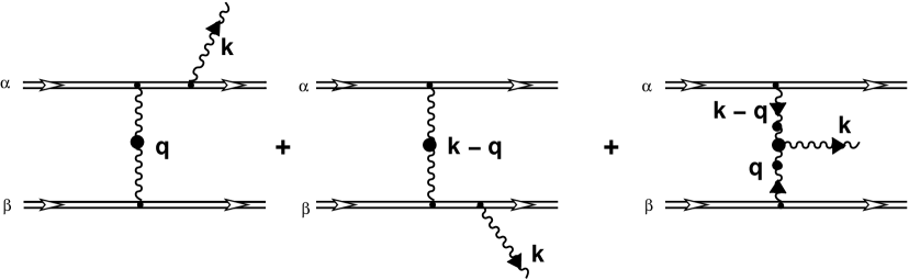
Figure 1: The simplest process of soft-gluon bremsstrahlung generating by color effective current (2.11). The blob stands for HTL resummation, and the double lines denote hard particles.

terms on the right-hand side of Eq. (2.12) is presented.

Thus we have shown that the effective current generating the lowest-order process of the induced gluon radiation from fast partons appears in the solution of the basic field equation (2.3) that defines interacting soft-gluon field $A_{\mu}$ in the form of an expansion in an initial value of color charges $Q_{0\alpha}$ and $Q_{0\beta}$. Based on this result and on the results of Paper I and Paper II also we can write out now more general structure of the effective current in the form of a functional expansion in a free field $A_{\mu}^{(0)}$ and color charges $Q_{0\alpha}$, $Q_{0\beta}$ generating the bremsstrahlung of arbitrary number of soft gluons for scattering of two hard color partons among themselves

$$\tilde{J}_{Q\mu}^{({\rm br})a}[A^{(0)}](k)=\tilde{J}_{Q\alpha\mu}^{(0)a}(k)+\tilde{J}_{Q\beta\mu}^{(0)a}(k)+K_{\mu}^{a}({\bf v}_{\alpha},{\bf v}_{\beta};{\bf x}_{0\alpha},{\bf x}_{0\beta},Q_{0\alpha},Q_{0\beta}|\,k)$$ (2.13)

$$+\!\sum\limits_{n=1}^{\infty}\!\int\!\!K_{\mu\mu_{1}\ldots\mu_{n}}^{aa_{1}\ldots a_{n}}({\bf v}_{\alpha},{\bf v}_{\beta};{\bf x}_{0\alpha},{\bf x}_{0\beta},Q_{0\alpha},Q_{0\beta}|\,k,-k_{1},\ldots,-k_{n})A^{(0)a_{1}\mu_{1}}(k_{1})\ldots A^{(0)a_{n}\mu_{n}}(k_{n})\!\!\prod_{s=1}^{n}\!dk_{s}.$$

The functions $K_{\mu\mu_{1}\ldots\mu_{n}}^{aa_{1}\ldots a_{n}},\,n=0,1,\ldots$ itself represent in general infinite series in expansion over color charges $Q_{0\alpha}$ and $Q_{0\beta}$. Thus, for example, for $K_{\mu}^{a}$ we have

$$K_{\mu}^{a}({\bf v}_{\alpha},{\bf v}_{\beta};{\bf x}_{0\alpha},{\bf x}_{0\beta},Q_{0\alpha},Q_{0\beta}|\,k)=K_{\mu}^{abc}({\bf v}_{\alpha},{\bf v}_{\beta};{\bf x}_{0\alpha},{\bf x}_{0\beta}|\,k)Q_{0\alpha}^{b}Q_{0\beta}^{c},$$ (2.14)

$$+\frac{1}{2!}\Bigl{\{}K_{\mu}^{abc_{1}c_{2}}({\bf v}_{\alpha},{\bf v}_{\beta};{\bf x}_{0\alpha},{\bf x}_{0\beta}|\,k)Q_{0\alpha}^{b}Q_{0\beta}^{c_{1}}Q_{0\beta}^{c_{2}}+K_{\mu}^{ab_{1}b_{2}c}({\bf v}_{\alpha},{\bf v}_{\beta};{\bf x}_{0\alpha},{\bf x}_{0\beta}|\,k)Q_{0\alpha}^{b_{1}}Q_{0\alpha}^{b_{2}}Q_{0\beta}^{c}\Bigr{\}}+\ldots\,.$$

Here, the first coefficient function $K_{\mu}^{abc}({\bf v}_{\alpha},{\bf v}_{\beta};\ldots|\,k)$ is explicitly defined by Eqs. (2.11), (2.12), and exact form of next-to-leading coefficient functions $K_{\mu}^{abc_{1}c_{2}}({\bf v}_{\alpha},{\bf v}_{\beta};\ldots|\,k)$ and $K_{\mu}^{ab_{1}b_{2}c}({\bf v}_{\alpha},{\bf v}_{\beta};\ldots|\,k)$, and their physical meaning will be given in Section 6.

3 Radiation intensity of soft gluon bremsstrahlung

In the expression for an effective current (2.13) without loss of generality one can set ${\bf x}_{0\alpha}=0$, and choose vector ${\bf x}_{0\beta}$ in the form ${\bf x}_{0\beta}=({\bf b},z_{0\beta})$, where two-dimensional vector ${\bf b}$ is orthogonal to relative velocity ${\bf v}_{\alpha}-{\bf v}_{\beta}$. Besides in the subsequent discussion a longitudinal component $z_{0{\beta}}$ also does not play any role and thus it can be set equal to zero. The energy of radiation field $E_{Q}^{ai}(k)=-i\omega\,^{\ast}{\cal D}^{i\nu}_{C}(k)\tilde{J}_{Q\nu}^{({\rm br})a}[A^{(0)}](k)+ik^{i}\,{}^{\ast}{\cal D}^{0\nu}_{C}(k)\tilde{J}_{Q\nu}^{({\rm br})a}[A^{(0)}](k)$, generated by the effective current, is defined by an expression

$$W({\bf b})=-(2\pi)^{4}\!\int\!d{\bf k}d\omega\!\int\!dQ_{0\alpha}dQ_{0\beta}\,\omega{\rm Im}\,\langle\tilde{J}^{({\rm br})\ast a}_{Q\mu}(k,{\bf b})\!\,^{\ast}{\cal D}^{\mu\nu}_{C}(k)\tilde{J}^{({\rm br})a}_{Q\nu}(k,{\bf b})\rangle.$$ (3.1)

Here,

$$dQ_{0\alpha,\beta}=\prod_{a=1}^{d_{A}}dQ_{0\alpha,\beta}^{a}\,\delta(Q_{0\alpha}^{a}Q_{0\beta}^{a}-C_{2}^{(\alpha,\beta)}),\quad d_{A}=N_{c}^{2}-1,$$

with the second order Casimir $C_{2}^{(\alpha,\beta)}$ for $\alpha\,(\beta)$ color particles; $\langle\cdot\rangle$ is an expectation value over the equilibrium ensemble. Eq. (3.1) represents a minimal extension of an corresponding expression in Abelian theory [50] taking into account a color degree of freedom of particles. The radiation energy (3.1) is a function of two-dimensional vector ${\bf b}$ being impact parameter in this case.

Let us define an expression for radiation intensity of soft gluon bremsstrahlung in passage of high-energy parton $\alpha$ through medium consisting of hard thermal partons of $\beta$ sort, using basic formula (3.1). Here we follow reasoning of Ginsburg and Tsytovich [50]. For simplicity we assume that particles $\beta$ are non-relativistic, their distribution over momentum ${\bf p}_{\beta}$ is given by distribution function $f_{{\bf p}_{\beta}}$. It is defined by formula

$$n_{\beta}=\!\int\!\!f_{{\bf p}_{\beta}}\,\frac{d{\bf p}_{\beta}}{(2\pi)^{3}}.$$

In this case radiation intensity is read

$${\cal I}=\int\!d{\bf b}\!\int\!f_{{\bf p}_{\beta}}\,\frac{d{\bf p}_{\beta}}{(2\pi)^{3}}\,W({\bf b})\,|{\bf v}_{\alpha}-{\bf v}_{\beta}|\equiv\left\langle\frac{dW({\bf b})}{dt}\right\rangle_{\!{\bf b}}.$$ (3.2)

We note once again that this expression defines a change of energy field in system for per time due to bremsstrahlung process. It equals (with opposite sign) change of kinetic energy of $\alpha$ particle and $\beta$ particles in medium on which nonelastic scattering arises. In this case when both particle $\alpha$ and particles $\beta$ radiate it is impossible in principle to separate a contribution of energy loss of particle $\alpha$ from a contribution of energy loss of particles $\beta$ in medium. In limiting case “frozen” $\beta$ particles only, when it can be neglected by its bremsstrahlung, Eq. (3.2) coincides with an expression for energy loss ${\cal I}|_{{\bf v}_{\beta}=0}=-dE/dt$, where $E$ is energy of a fast parton $\alpha$.

One can define a probability of bremsstrahlung. Let us refer the probability to unit intervals of momentum of emitted quantum $d{\bf k}/(2\pi)^{3}$ and transferred momentum $d{\bf q}/(2\pi)^{3}$. The probability of bremsstrahlung ${\it w}_{{\bf p}_{\alpha},{\bf p}_{\beta}}({\bf k},{\bf q})$ is defined by a simple formula

$$\left\langle\frac{dW({\bf b})}{dt}\right\rangle_{\!{\bf b}}=\int\!\omega({\bf k}){\it w}_{{\bf p}_{\alpha},{\bf p}_{\beta}}({\bf k},{\bf q})\,\frac{f_{{\bf p}_{\beta}}d{\bf p}_{\beta}}{(2\pi)^{3}}\,\frac{d{\bf k}d{\bf q}}{(2\pi)^{6}}\,\,\delta(\omega({\bf k})-{\bf k}\cdot{\bf v}_{\alpha}-{\bf q}\cdot({\bf v}_{\beta}-{\bf v}_{\alpha})).$$ (3.3)

Now we obtain an expression for radiation intensity generated by the lowest-order process of the induced gluon radiation (Fig. 1). We substitute an effective current (2.11) into the right-hand side of Eq. (3.1). Using an expression for propagator in Coulomb gauge (2.6) and averaging rules over initial values of color charges

$$\int\!dQ_{0\alpha}\,Q_{0\alpha}^{a}Q_{0\alpha}^{b}=\frac{C_{2}^{(\alpha)}}{d_{A}}\,\delta^{ab},\quad\int\!dQ_{0\beta}\,Q_{0\beta}^{a}Q_{0\beta}^{b}=\frac{C_{2}^{(\beta)}}{d_{A}}\,\delta^{ab},$$

from Eq. (3.1) we find

$$W({\bf b})=\frac{1}{(2\pi)^{2}}\,\biggl{(}\frac{{\alpha}_{s}}{\pi}\biggr{)}^{\!3}\!C_{A}\Biggl{(}\frac{C_{2}^{(\alpha)}C_{2}^{(\beta)}}{d_{A}}\Biggr{)}\!\sum_{\zeta=1,2}\!\int\!d{\bf k}d\omega\,\omega\,{\rm Im}(^{\ast}{\!\Delta}^{t}(k))|\,{\rm e}^{i}(\hat{\bf k},\zeta)K^{i}({\bf v}_{\alpha},{\bf v}_{\beta};{\bf b}|\,k)|^{\,2}$$ (3.4)

$$\hskip 8.5359pt-\,\frac{1}{(2\pi)^{2}}\,\biggl{(}\frac{{\alpha}_{s}}{\pi}\biggr{)}^{\!3}\!C_{A}\Biggl{(}\frac{C_{2}^{(\alpha)}C_{2}^{(\beta)}}{d_{A}}\Biggr{)}\!\sum_{\zeta=1,2}\!\int\!d{\bf k}d\omega\,\omega\,{\rm Im}(^{\ast}{\!\Delta}^{l}(k))|\,K^{0}({\bf v}_{\alpha},{\bf v}_{\beta};{\bf b}|\,k)|^{\,2}.$$

Here, $\alpha_{s}\equiv g^{2}/4\pi$. The first term on the right-hand side is connected with bremsstrahlung of transverse gluon, and a second one is associated with bremsstrahlung of longitudinal gluon. For transverse mode we introduce polarization vectors ${\rm e}^{i}(\hat{\bf k},\zeta),\,\zeta=1,2$ possessing properties

$${\bf k}\cdot{\bf e}(\hat{\bf k},\zeta)=0,\quad{\bf e}^{\ast}(\hat{\bf k},\zeta)\cdot{\bf e}(\hat{\bf k},\zeta^{\prime})=\delta_{\zeta{\zeta}^{\prime}}.$$

Three-dimensional transverse projector in (2.6) is associated with polarization vectors by relation

$$P^{ij}(\hat{\bf k})=(\delta^{ij}-\hat{k}^{i}\hat{k}^{j})=\sum_{\zeta=1,2}{\rm e}^{\ast i}(\hat{\bf k},\zeta)\,{\rm e}^{j}(\hat{\bf k},\zeta).$$ (3.5)

Let us consider in more detail an expressions $|{\rm e}^{i}K^{i}|^{\,2}$ and $|K^{0}|^{\,2}$ on the right-hand side of Eq. (3.4). Due to Eq. (2.12) the first expression can be presented in the form

$$|{\rm e}^{i}(\hat{\bf k},\zeta)K^{i}({\bf v}_{\alpha},{\bf v}_{\beta};{\bf b}|\,k)|^{\,2}\!=\!\left|\int\!{\rm e}^{i{\bf q}\cdot{\bf b}}{\rm e}^{i}(\hat{\bf k},\zeta){\cal K}^{i}({\bf v}_{\alpha},{\bf v}_{\beta}|\,k,q)\delta(\omega\!-\!{\bf v}_{\beta}\!\cdot\!{\bf q}\!-\!{\bf v}_{\alpha}\!\cdot\!({\bf k}\!-\!{\bf q}))d{\bf q}\right|^{\,2}_{q_{0}={\bf v}_{\beta}\cdot{\bf q}}$$

$$=\int\!{\rm e}^{i({\bf q}-{\bf q}^{\prime})\cdot{\bf b}}\Bigl{[}({\rm e}^{i}(\hat{\bf k},\zeta){\cal K}^{i}({\bf v}_{\alpha},{\bf v}_{\beta}|\,k,q))({\rm e}^{j}(\hat{\bf k},\zeta){\cal K}^{j}({\bf v}_{\alpha},{\bf v}_{\beta}|\,k,q))^{\ast}\Bigr{]}_{q_{0}={\bf v}_{\beta}\cdot{\bf q}}$$ (3.6)

$$\times\,\delta(\omega-{\bf v}_{\beta}\cdot{\bf q}-{\bf v}_{\alpha}\cdot({\bf k}-{\bf q}))\,\delta(({\bf v}_{\alpha}-{\bf v}_{\beta})\cdot({\bf q}-{\bf q}^{\prime}))d{\bf q}d{\bf q}^{\prime},$$

where

$${\cal K}^{\mu}({\bf v}_{\alpha},{\bf v}_{\beta}|\,k,q)=\frac{v_{\alpha}^{\mu}}{v_{\alpha}\cdot q}\,(v_{\alpha\nu}\!\,^{\ast}{\cal D}_{C}^{\nu\nu^{\prime}}(q)v_{\beta\nu^{\prime}})-\frac{v_{\beta}^{\mu}}{v_{\beta}\cdot(k-q)}\,(v_{\beta\nu}\!\,^{\ast}{\cal D}_{C}^{\nu\nu^{\prime}}(k-q)v_{\alpha\nu^{\prime}})$$

$$+\,^{\ast}\Gamma^{\mu\nu\lambda}(k,-q,-k+q)\,\,^{\ast}{\cal D}_{C\nu\nu^{\prime}}(q)v_{\beta}^{\nu^{\prime}}\,{}^{\ast}{\cal D}_{C\lambda\lambda^{\prime}}(k-q)v_{\alpha}^{\lambda^{\prime}}.$$ (3.7)

In the last line of Eq. (3.6) delta-function $\delta(({\bf v}_{\alpha}-{\bf v}_{\beta})\cdot({\bf q}-{\bf q}^{\prime}))=\delta(q_{\|}-q^{\prime}_{\|})/|{\bf v}_{\alpha}-{\bf v}_{\beta}|$ enables the integration over longitudinal component of vector ${\bf q}^{\prime}=({\bf q}_{\perp}^{\prime},q_{\|}^{\prime})$ to be performed. For deriving radiation intensity we multiply (3.4) by $f_{{\bf p}_{\beta}}d{\bf p}_{\beta}/(2\pi)^{3}|{\bf v}_{\alpha}-{\bf v}_{\beta}|d{\bf b}$ and integrate over ${\bf p}_{\beta}$ and ${\bf b}$. We perform integration over impact parameter ${\bf b}$ with the help of expression

$$\int\!{\rm e}^{i({\bf q}-{\bf q}^{\prime})\cdot{\bf b}}d{\bf b}=(2\pi)^{2}\delta^{(2)}(({\bf q}-{\bf q}^{\prime})_{\perp}).$$ (3.8)

The Eq. (3.8) enables us to performe complete integration over $d{\bf q}^{\prime}$ in (3.6) and thus to define initial for subsequent analysis expression of radiation intensity for the bremsstrahlung process dipected on Fig. 1

$$\left\langle\frac{dW({\bf b})}{dt}\right\rangle_{\!{\bf b}}=-\biggl{(}\frac{{\alpha}_{s}}{\pi}\biggr{)}^{\!3}\!C_{A}\Biggl{(}\frac{C_{2}^{(\alpha)}C_{2}^{(\beta)}}{d_{A}}\Biggr{)}\Biggl{(}\int\!{\bf p}_{\beta}^{2}f_{|{\bf p}_{\beta}|}\,\frac{d|{\bf p}_{\beta}|}{2\pi^{2}}\Biggr{)}$$ (3.9)

$$\times\,\Biggl{[}\int\!\frac{d\Omega_{{\bf v}_{\beta}}}{4\pi}\!\sum_{\zeta=1,2}\!\int\!d{\bf k}d\omega\,\omega\,{\rm Im}(^{\ast}{\!\Delta}^{t}(k))\int\!d{\bf q}\,|{\rm e}^{i}(\hat{\bf k},\zeta){\cal K}^{i}({\bf v}_{\alpha},{\bf v}_{\beta}|\,k,q)|^{\,2}$$

$$\times\,\delta(\omega-{\bf v}_{\beta}\cdot{\bf q}-{\bf v}_{\alpha}\cdot({\bf k}-{\bf q}))+\Bigl{(}\,^{\ast}{\!\Delta}^{t}(k)\rightarrow\,^{\ast}{\!\Delta}^{l}(k),\;{\rm e}^{i}{\cal K}^{i}\rightarrow\sqrt{\frac{k^{2}}{{\bf k}^{2}}}\,{\cal K}^{0}\Bigr{)}\Biggr{]}_{q^{0}=({\bf v}_{\beta}\cdot{\bf q})}.$$

If there are several sorts of thermal partons, then on the right-hand side of Eq. (3.9) it should be summarize over $\beta$. In notation (3.9) we assume isotropy of a medium, i.e. $f_{{\bf p}_{\beta}}=f_{|{\bf p}_{\beta}|}$.

Now we consider a special case of Eq. (3.9). Let us define the radiation intensity caused by bremsstrahlung of real quantum of oscillations, i.e. oscillations lying on mass-shell. For this purpose, for a weak-absorption medium, when ${\rm Im}(^{\ast}{\!\Delta}^{\!-1\,t,\,l}(k))\rightarrow 0$, we can approximate imaginary part of scalar propagators in the following way

$${\rm Im}(^{\ast}{\!\Delta}^{t,\,l}(k))\simeq-\pi\,{\rm sign}(\omega)\,\frac{{\rm Z}_{t,\,l}({\bf k})}{2\omega_{\bf k}^{t,\,l}}\,[\,\delta(\omega-\omega_{\bf k}^{t,\,l})+\delta(\omega+\omega_{\bf k}^{t,\,l})],$$ (3.10)

where ${\rm Z}_{t,\,l}({\bf k})$ are the residues of appropriate scalar propagators ${}^{\ast}{\!\Delta}^{\!-1\,t,\,l}(k)$ at the poles and $\omega_{\bf k}^{t,\,l}\equiv{\omega}^{t,\,l}({\bf k})$ are the dispersion relations for transverse and longitudinal modes. The term with $\delta(\omega+\omega_{\bf k}^{t,\,l})$ on the right-hand side of Eq. (3.10) takes into consideration not emission, but absorption of oscillation. Substituting (3.10) into (3.9) and omitting the last contribution after integration over $d\omega$, we find instead of (3.9)

$$\left\langle\frac{dW({\bf b})}{dt}\right\rangle_{\!{\bf b}}=\frac{{\alpha}_{s}^{3}}{\pi^{2}}\!\sum_{\beta=q,\,\bar{q},\,{\rm g}}\!C_{A}\Biggl{(}\frac{C_{2}^{(\alpha)}C_{2}^{(\beta)}}{d_{A}}\Biggr{)}\Biggl{(}\int\!{\bf p}_{\beta}^{2}f_{|{\bf p}_{\beta}|}\,\frac{d|{\bf p}_{\beta}|}{2\pi^{2}}\Biggr{)}$$ (3.11)

$$\times\Biggl{[}\int\!\frac{d\Omega_{{\bf v}_{\beta}}}{4\pi}\!\sum_{\zeta=1,2}\!\int\!d{\bf k}\,\omega_{\bf k}^{t}\Biggl{(}\frac{{\rm Z}_{t}({\bf k})}{2\omega_{\bf k}^{t}}\Biggr{)}\!\int\!d{\bf q}\,|\,{\rm e}^{i}(\hat{\bf k},\zeta){\cal K}^{i}({\bf v}_{\alpha},{\bf v}_{\beta}|\,k,q)|^{\,2}_{\,{\rm on-shell}}$$

$$\times\,\delta(\omega_{\bf k}^{t}-{\bf v}_{\beta}\cdot{\bf q}-{\bf v}_{\alpha}\cdot({\bf k}-{\bf q}))+\Bigl{(}t\rightarrow l,\;{\rm e}^{i}{\cal K}^{i}\rightarrow\sqrt{\frac{k^{2}}{{\bf k}^{2}}}\,{\cal K}^{0}\Bigr{)}\Biggr{]}_{q^{0}=({\bf v}_{\beta}\cdot{\bf q})}.$$

Comparing the last expression with (3.3) we derive an explicit form for the probabilities of soft-gluon bremsstrahlung

$${\it w}_{{\bf p}_{\alpha},{\bf p}_{\beta}}^{t}({\bf k},{\bf q})=4(2\pi)^{4}\alpha_{s}^{3}C_{A}\Biggl{(}\frac{C_{2}^{(\alpha)}C_{2}^{(\beta)}}{d_{A}}\Biggr{)}\Biggl{(}\frac{{\rm Z}_{t}({\bf k})}{2\omega_{\bf k}^{t}}\Biggr{)}\!\sum_{\zeta=1,2}\!|\,{\rm e}^{i}(\hat{\bf k},\zeta){\cal K}^{i}({\bf v}_{\alpha},{\bf v}_{\beta}|\,k,q)|^{\,2}_{\,\omega=\omega_{\bf k}^{t},\,q_{0}={\bf v}_{\beta}\cdot{\bf q}},$$ (3.12)

$${\it w}_{{\bf p}_{\alpha},{\bf p}_{\beta}}^{l}({\bf k},{\bf q})=4(2\pi)^{4}\alpha_{s}^{3}C_{A}\Biggl{(}\frac{C_{2}^{(\alpha)}C_{2}^{(\beta)}}{d_{A}}\Biggr{)}\Biggl{(}\frac{{\rm Z}_{l}({\bf k})}{2\omega_{\bf k}^{l}}\Biggr{)}\!\Biggl{(}\frac{k^{2}}{{\bf k}^{2}}\Biggr{)}|{\cal K}^{0}({\bf v}_{\alpha},{\bf v}_{\beta}|\,k,q)|^{\,2}_{\,\omega=\omega_{\bf k}^{l},\,q_{0}={\bf v}_{\beta}\cdot{\bf q}}.$$

The expressions (3.11), (3.12) were obtained with the assumption that QGP represents a system of non-relativistic thermal partons. In this case only the use of the impact parameter and averaging over it, is valid. It enables us to diagonalize the product of amplitude ${\rm e}^{i}{\cal K}^{i}$ and complex conjugate amplitude (Eq. (3.6)) in the ${\bf q},\,{\bf q}^{\prime}$ variables, and to write the probability in the simple form (3.12). In the work [50] a possible way of extension of this approach to the case of arbitrary moving thermal particles, was suggested. It consists in construction of subsequent Lorentz transformations for particles group with momenta in interval $({\bf p}_{\beta},{\bf p}_{\beta}+d{\bf p}_{\beta})$ at rest, where Eq. (3.11) is true. However practical use of this idea is very difficult. In work by Akopian and Tsytovich [5] for the case when both particle $\alpha$ and particles $\beta$ are ultra-relativistic, the probability of bremsstrahlung (3.12) for ordinary plasma was derived by direct computations with use of dynamical equation without notion of impact parameter. It gives some ground to suppose that expressions (3.11), (3.12) hold for ultra-relativistic high-temperature plasma also.

4 Approximation of static color center

Let us analyze an expression for gluon radiation intensity (3.11) in the case when target particle is modeled by static screened potential $({\bf{\bf v}}_{\beta}=0)$, and HTL-correction $\delta\Gamma_{3g}$ to bare three-gluon vertex can be neglected. For simplicity we restrict our consideration to the case of transverse gluon radiation. At first we consider integral over momentum transfer ${\bf q}$ on the right-hand side of Eq. (3.11) presented as

$$\int\!d{\bf q}_{\perp}dq_{\|}\left|\,{\rm e}^{i}(\hat{\bf k},\zeta){\cal K}^{i}({\bf v}_{\alpha},0|\,k,q)\right|^{\,2}_{\,\omega=\omega^{t}_{\bf k},\;q_{0}=0}\delta(\omega^{t}_{\bf k}-{\bf v}_{\alpha}\cdot{\bf k}+v_{\alpha}q_{\|}),$$ (4.1)

where ${\bf q}_{\perp}$ and $q_{\|}$ are transverse and longitudinal components of momentum transfer with respect to velocity ${\bf v}_{\alpha}$, correspondingly, and $v_{\alpha}\equiv|{\bf v}_{\alpha}|.$ Based on an explicit expression for ${\cal K}^{i}({\bf v}_{\alpha},{\bf v}_{\beta}|\,k,q)$ (Eq. (3.7)) and limiting static expression for propagator

$$\,{}^{\ast}{\cal D}^{00}_{C}(0,{\bf q})=\frac{1}{{\bf q}^{2}+\mu_{D}^{2}},$$ (4.2)

where $\mu_{D}^{2}$ is Debay screening mass, and performing integration over $dq_{\|}$, we find instead of (4.1)

$$\frac{1}{v_{\alpha}}\int\!d{\bf q}_{\perp}\frac{1}{\left({\bf q}_{\perp}^{2}+\mu_{D}^{2}+\displaystyle\frac{1}{v_{\alpha}^{2}}(\omega_{\bf k}^{t}-{\bf v}_{\alpha}\cdot{\bf k})^{2}\right)^{2}}$$ (4.3)

$$\times\left|\,\frac{{\bf e}\cdot{\bf v}_{\alpha}}{\omega_{\bf k}^{t}-{\bf v}_{\alpha}\cdot{\bf k}}+{\rm e}^{i}(\hat{\bf k},\zeta)\Gamma^{i0\mu}(k,-q,-k+q)\!\,^{\ast}{\cal D}_{C\mu\mu^{\prime}}(k-q)v_{\alpha}^{\mu^{\prime}}\right|^{\,2}_{\,q_{0}=0,\;q_{\|}=-\frac{1}{v_{\alpha}}(\omega_{\bf k}^{t}-{\bf v}_{\alpha}\cdot{\bf k})}.$$

Here, for brevity we use a notation ${\bf e}\equiv{\bf e}(\hat{\bf k},\zeta)$. We note that in our approach in deciding on Coulomb gauge, a contribution of thermal parton $\beta$ (the second term in function ${\cal K}^{i}$, Eq. (3.7)) to bremsstrahlung of transverse soft gluon is exactly equal to zero. However here, there is a possibility of radiation of longitudinal plasmon from target $\beta$. Let us consider a difference $\omega_{\bf k}^{t}-{\bf v}_{\alpha}\cdot{\bf k}$. We approximate a spectrum of transverse oscillations $\omega_{\bf k}^{t}$ in the limit of $|{\bf k}_{\perp}|\ll k_{\|}$ by standard expression

$$\omega_{\bf k}^{t}\simeq\sqrt{{\bf k}^{2}+m_{g}^{2}}\simeq k_{\|}+\frac{{\bf k}^{2}_{\perp}+m_{g}^{2}}{2k_{\|}}.$$

Here, $m_{g}^{2}$ is an effective gluon mass square, depending on temperature of the system, $m_{g}^{2}=3\omega_{pl}^{2}/2$, where $\omega_{pl}^{2}=g^{2}T^{2}(N_{f}+2N_{c})/18$ is plasma frequency square.

Besides, for ultrarelativistic particle $\alpha$ with energy $E$ and finite mass $M$, we have

$$v_{\alpha}\simeq 1-\frac{M^{2}}{2E^{2}}.$$ (4.4)

Based on above-mentioned we can write

$$\omega_{\bf k}^{t}-{\bf v}_{\alpha}\cdot{\bf k}\simeq\frac{{\bf k}_{\perp}^{2}+m_{g}^{2}+x^{2}M^{2}}{2\omega},\;x\equiv\frac{\omega}{E}.$$ (4.5)

Furthermore from a condition of transversity we obtain $e_{\|}\simeq-({\bf k}_{\perp}\cdot{\bf{\bf e}}_{\perp})/\omega$ whence it follows

$${\bf e}\cdot{\bf v}_{\alpha}\simeq-v_{\alpha}\,\frac{{\bf k}_{\perp}\cdot{\bf e}_{\perp}}{\omega}.$$ (4.6)

Taking into account (4.5) and (4.6) we can write a first term in expression under module squared in (4.3) as

$$\frac{{\bf e}\cdot{\bf v}_{\alpha}}{\omega_{\bf k}^{t}-{\bf v}_{\alpha}\cdot{\bf k}}\simeq-2v_{\alpha}\,\frac{{\bf k}_{\perp}\cdot{\bf e}_{\perp}}{{\bf k}_{\perp}^{2}+m_{g}^{2}+x^{2}M^{2}},$$ (4.7)

and Coulomb factor reads

$$\frac{1}{\left({\bf q}_{\perp}^{2}+\mu_{D}^{2}+\displaystyle\frac{1}{v_{\alpha}^{2}}(\omega_{\bf k}^{t}-{\bf v}_{\alpha}\cdot{\bf k})^{2}\right)^{2}}\simeq\frac{1}{({\bf q}^{2}_{\perp}+\mu_{D}^{2}+l_{f}^{-2})^{2}}.$$ (4.8)

Here, $l_{f}=v_{\alpha}\tau_{f}$, where $\tau_{f}\equiv 2\omega/({\bf k}_{\perp}^{2}+m_{g}^{2}+x^{2}M^{2})$ is finite formation time with regard to temperature induced gluon mass and finite mass of projectile $\alpha$.

Let us consider now a contribution to matrix element associated with bare three-gluon vertex. Taking into account structure of propagator in the Coulomb gauge (Eq. (2.6)) and approximation (4.6), we can present this contribution as

$$-2\,\frac{\{\omega^{2}-({\bf k}-{\bf q})^{2}\}}{({\bf k}-{\bf q})^{2}}\,({\bf e}\cdot{\bf q})\,^{\ast}\!\Delta^{l}(k-q)+2\omega\left\{\,-v_{\alpha}\,\frac{{\bf k}_{\perp}\cdot{\bf e}_{\perp}}{\omega}+\omega\,\frac{{\bf e}\cdot{\bf q}}{({\bf k}-{\bf q})^{2}}\right\}\!\,^{\ast}\!\Delta^{t}(k-q).$$ (4.9)

Furthermore by virtue of (4.5) we have

$${\bf e}\cdot{\bf q}={\bf e}_{\perp}\cdot{\bf q}_{\perp}+e_{\|}q_{\|}\simeq{\bf e}_{\perp}\cdot\left(\,{\bf q}_{\perp}+\frac{{\bf k}_{\perp}}{\omega}\frac{1}{l_{f}}\right)\simeq{\bf e}_{\perp}\cdot{\bf q}_{\perp}$$

under condition $|{\bf k}_{\perp}|/{\omega}l_{f}\ll|{\bf q}_{\perp}|$. Besides we have $({\bf k}-{\bf q})^{2}=({\bf k}-{\bf q})^{2}_{\perp}+\omega^{2}/v_{\alpha}^{2}\simeq\omega^{2}/v_{\alpha}^{2}$, when $\omega^{2}/v_{\alpha}^{2}\!\gg\!({\bf k}-{\bf q})^{2}_{\perp}$. By this mean expression (4.9) can be replaced by approximate one

$$2\,\frac{x^{2}M^{2}+({\bf k}-{\bf q})^{2}_{\perp}}{\omega^{2}}\,({\bf e}_{\perp}\cdot{\bf q}_{\perp})\,^{\ast}\!\Delta^{l}(k-q)+2v_{\alpha}({\bf e}_{\perp}\cdot(v_{\alpha}{\bf q}-{\bf k})_{\perp})\,^{\ast}\!\Delta^{t}(k-q).$$

Here, a first term connected with a contribution from longitudinal virtual oscillation is suppressed with respect to a second term by small factor and it can be omitted.

Let us consider transverse gluon propagator $\,{}^{\ast}\!\Delta^{t}(\omega,{\bf k}-{\bf q})$. Its explicit expression in hard thermal loop approximation is

$$\,{}^{\ast}\!\Delta^{t}(\omega,{\bf k}-{\bf q})=\left[\,\omega^{2}-({\bf k}-{\bf q})^{2}-\frac{1}{2}\,\mu_{D}^{2}\Biggl{\{}\frac{\omega^{2}}{({\bf k}-{\bf q})^{2}}-\frac{\omega^{2}-({\bf k}-{\bf q})^{2}}{({\bf k}-{\bf q})^{2}}\,F\Biggl{(}\frac{\omega}{|{\bf k}-{\bf q}|}\Biggr{)}\!\Biggr{\}}\right]^{-1},$$

where

$$F(z)\equiv\frac{z}{2}\,\bigg{[}\ln\bigg{|}\frac{1+z}{1-z}\bigg{|}-i\pi\theta(1-|z|)\bigg{]}.$$

By making use approximations

$$({\bf k}-{\bf q})^{2}\simeq{\bf k}^{2}+({\bf k}-{\bf q})^{2}_{\perp}+m_{g}^{2}+x^{2}M^{2},\quad\frac{\omega}{|{\bf k}-{\bf q}|}\simeq 1-\,\frac{[({\bf k}-{\bf q})^{2}_{\perp}+x^{2}M^{2}]}{2{\bf k}^{2}},$$ (4.10)

we derive for transverse propagator

$$\,{}^{\ast}\!\Delta^{t}(\omega,{\bf k}-{\bf q})\!\simeq\!-\!\left[({\bf k}\!-\!{\bf q})^{2}_{\perp}\!+\!x^{2}M^{2}\!+\!\frac{1}{2}\mu_{D}^{2}\Biggl{\{}1\!+\!\frac{[({\bf k}\!-\!{\bf q})^{2}_{\perp}\!+\!x^{2}M^{2}]}{2{\bf k}^{2}}\Biggl{(}\!\ln\frac{4{\bf k}^{2}}{[({\bf k}\!-\!{\bf q})^{2}_{\perp}\!+\!x^{2}M^{2}]}\!-\!i\pi\!\Biggr{)}\!\!\Biggr{\}}\right]^{-1}\!\!.$$

The factor before a logarithm on the right-hand side of the last expression is a small owing to ${\bf k}^{2}\gg({\bf k}-{\bf q})^{2}_{\perp}+x^{2}M^{2}$. On the other hand, the logarithm can be large by the same condition. Therefore this term can be discarded under more severe constraint for the magnitude of momentum $|{\bf k}|$:

$$\epsilon\ln\epsilon\ll 1,\quad\epsilon\equiv[({\bf k}-{\bf q})^{2}_{\perp}+x^{2}M^{2}]/{\bf k}^{2}.$$

Under the last condition with allowance for $\mu_{D}^{2}/2=m_{g}^{2}$ we derive finally expression for transverse gluon propagator

$$\,{}^{\ast}\!\Delta^{t}(\omega,{\bf k}-{\bf q})\simeq-\frac{1}{({\bf k}-{\bf q})^{2}_{\perp}+m_{g}^{2}+x^{2}M^{2}}.$$ (4.11)

By this means a contribution to matrix element connected with bare three-gluon vertex in this high-frequency limit can be presented as

$${\rm e}^{i}\Gamma^{i0\mu}(k,-q,-k+q)\!\,^{\ast}{\cal D}_{C\mu\mu^{\prime}}(k-q)v_{\alpha}^{\mu^{\prime}}\simeq-2v_{\alpha}\,\frac{{\bf e}_{\perp}\cdot(v_{\alpha}{\bf q}-{\bf k})_{\perp}}{({\bf k}-{\bf q})^{2}_{\perp}+m_{g}^{2}+x^{2}M^{2}}.$$ (4.12)

In this approximation the residue $Z_{t}({\bf k})$ can be replaced by unit.

With regard to (4.7), (4.8) and (4.12) the expression for energy loss of parton $\alpha$, associated with bremsstrahlung of soft transverse gluon, takes following form within the potential model

$$\left(-\frac{dE}{dt}\right)^{\!t}=2\pi\biggl{(}\,\frac{\alpha_{s}}{\pi}\biggr{)}^{\!3}v_{\alpha}E\,C_{\!A}\!\sum\limits_{\beta=q\!,\,\bar{q}\!,\,{\rm g}}\left(\frac{C_{2}^{(\alpha)}C_{2}^{(\beta)}}{d_{A}}\right)n_{\beta}\sum\limits_{\zeta=1,2}\int\!d{\bf k}_{\perp}\!\int\!dx$$ (4.13)

$$\times\!\int\!d{\bf q}_{\perp}\,\frac{1}{({\bf q}^{2}_{\perp}+\mu_{D}^{2}+l_{f}^{-2})^{2}}\,\left|\,{\bf e}_{\perp}({\bf k},\zeta)\cdot\Biggl{(}\frac{{\bf k}_{\perp}}{{\bf k}_{\perp}^{2}+m_{g}^{2}+x^{2}M^{2}}+\frac{(v_{\alpha}{\bf q}-{\bf k})_{\perp}}{({\bf k}-{\bf q})^{2}_{\perp}+m_{g}^{2}+x^{2}M^{2}}\Biggr{)}\right|^{\,2}.$$

The expression (4.13) takes into account the QCD Ter-Mikaelian effect associated with existence of an effective gluon mass $m_{g}$, depending on the temperature $T$. As was mentioned in Introduction for hot QCD plasma this effect was first considered by Kämpfer and Pavlenko [46]. As distinct from this work, in our paper the effective gluon mass appears not only in the first term of matrix element, but also in the second one corresponding to the radiation from gluon line via the triple vertex. Besides this expression takes into account mass finiteness of the projectile (mass effect) in according with expression obtained by Djordjevic and Gyulassy [67] for energy loss of heavy quarks.

Let us consider more closely the expression (4.13). First of all we define conditions wherein a term $l_{f}^{-2}$ in Coulomb factor $1/({\bf q}^{2}_{\perp}+\mu_{D}^{2}+l_{f}^{-2})^{2}$ can be neglected. The requirement $\mu_{D}^{2}\gg l_{f}^{-2}$ results in

$$\frac{{\bf k}_{\perp}^{2}}{2\omega}\ll\mu_{D},\quad\frac{1}{4}\,\mu_{D}\ll\omega\ll 2\gamma^{2}\mu_{D},$$ (4.14)

where we enter Lorentz-factor $\gamma=E/M$. Performing summation over polarization state of radiated transverse gluon, we rewrite the Eq. (4.13) as integral over frequency $\omega$

$$\left(-\frac{dE}{dt}\right)^{\!t}=2\pi\biggl{(}\,\frac{\alpha_{s}}{\pi}\biggr{)}^{\!3}v_{\alpha}C_{\!A}\!\sum\limits_{\beta=q,\,\bar{q},\,{\rm g}}\left(\frac{C_{2}^{(\alpha)}C_{2}^{(\beta)}}{d_{A}}\right)\!n_{\beta}\!\int\!d\omega\,\Bigl{\{}{\cal T}_{1}(\omega)+{\cal T}_{2}(\omega)+{\cal T}_{3}(\omega)\Bigr{\}},$$

where

$${\cal T}_{1}(\omega)=\int\!d{\bf k}_{\perp}\!\int\!d{\bf q}_{\perp}\,\frac{1}{({\bf q}^{2}_{\perp}+\mu_{D}^{2}+l_{f}^{-2})^{2}}\,\frac{{\bf k}^{2}_{\perp}}{({\bf k}^{2}_{\perp}+\tilde{m}_{g}^{2})^{2}},\hskip 122.34692pt$$

$${\cal T}_{2}(\omega)=\int\!d{\bf k}_{\perp}\!\int\!d{\bf q}_{\perp}\,\frac{-2}{({\bf q}^{2}_{\perp}+\mu_{D}^{2}+l_{f}^{-2})^{2}}\,\frac{{\bf k}_{\perp}\cdot({\bf k}-{\bf q})_{\perp}}{({\bf k}^{2}_{\perp}+\tilde{m}_{g}^{2})(({\bf k}-{\bf q})_{\perp}^{2}+\tilde{m}_{g}^{2})},\hskip 14.22636pt$$ (4.15)

$${\cal T}_{3}(\omega)=\!\int\!d{\bf k}_{\perp}\!\int\!d{\bf q}_{\perp}\,\frac{1}{({\bf q}^{2}_{\perp}+\mu_{D}^{2}+l_{f}^{-2})^{2}}\,\frac{({\bf k}-{\bf q})_{\perp}^{2}}{(({\bf k}-{\bf q})_{\perp}^{2}+\tilde{m}_{g}^{2})^{2}}.\hskip 93.89418pt$$

Here, for brevity we denote $\tilde{m}_{g}^{2}\equiv m_{g}^{2}+\omega^{2}\gamma^{-2}$. Now we consider a function ${\cal T}_{1}(\omega)$. In conditions of (4.14) a simple calculation of two-dimensional integrals $\int\!d{\bf k}_{\perp}\!\int\!d{\bf q}_{\perp}$ leads to

$${\cal T}_{1}(\omega)\simeq\frac{\pi^{2}}{\mu_{D}^{2}}\left\{\ln\Biggl{[}\frac{{\bf k}^{2}_{\perp\,{\rm max}}+\tilde{m}_{g}^{2}}{\tilde{m}_{g}^{2}}\Biggr{]}-1\right\}.$$ (4.16)

We introduce cut-off ${\bf k}^{2}_{\perp\,{\rm max}}$ on upper limit for integration over $d{\bf k}^{2}_{\perp}$. As will be shown below the divergent term in a sum of three expressions (4.15), is exactly cancelled. Here we draw attention to the following circumstance. If we keep the term $l_{f}^{-2}$ in Coulomb factor, then in this case integrating leads to finite expression by convergence of integral over $d|{\bf k}_{\perp}|$. For conditions (4.14) we will have instead of (4.16)

$${\cal T}_{1}(\omega)\simeq\frac{\pi^{2}}{\mu_{D}^{2}}\left\{\ln\Biggl{[}\frac{2\gamma^{2}\omega\mu_{D}}{\omega^{2}+\gamma^{2}m_{g}^{2}}\Biggr{]}-1+\,\frac{\omega^{2}+\gamma^{2}m_{g}^{2}}{2\gamma^{2}\omega\mu_{D}}\,\Biggl{(}\frac{\pi}{2}-\arctan\Biggl{[}\frac{\omega^{2}+\gamma^{2}m_{g}^{2}}{2\gamma^{2}\omega\mu_{D}}\Biggr{]}\Biggr{)}\!\right\}.$$

In particular in a frequencies region $\mu_{D}/4\ll\omega\ll\gamma m_{g}$ it follows

$${\cal T}_{1}(\omega)\simeq\frac{\pi^{2}}{\mu_{D}^{2}}\left\{\ln\Biggl{(}\frac{4\omega}{\mu_{D}}\Biggr{)}-1+\,\Biggl{(}\frac{\mu_{D}}{4\omega}\Biggr{)}^{\!2}+\,\ldots\right\}.$$

In this region a dependence on Lorentz-factor vanishes.

Finally, in asymptotic region $\omega\gg 2\gamma^{2}\mu_{D}$ we have

$${\cal T}_{1}(\omega)\simeq\frac{\pi^{2}}{\mu_{D}^{2}}\,\frac{1}{6}\Biggl{(}\frac{2\gamma^{2}\mu_{D}}{\omega}\Biggr{)}^{\!2}.$$

Here, we note a strong suppression of spectral density.

Such allowance for finiteness (inverse) formation length enables us not only to perform more accurate integration providing its finiteness, but gives also a possibility to analyze a behavior of spectral density outside of framework of restriction (4.14). However here, a problem connected with necessity of the keeping of terms of higher order smallness over ${\bf k}^{2}_{\perp},\,{\bf q}^{2}_{\perp}\,etc$ arises in an approximation scheme, that results in Eq. (4.13). Besides for allowance of finiteness of $l_{f}^{-2}$ for deriving of the remaining expressions of ${\cal T}_{2}(\omega)$ and ${\cal T}_{3}(\omega)$, calculation complexities arise. In conditions of requirements (4.14) before integrating, these formulas can be introduced in the form

$${\cal T}_{2}(\omega)\simeq-2\frac{\pi^{2}}{\mu_{D}^{2}}\ln\Biggl{[}\frac{{\bf k}^{2}_{\perp\,{\rm max}}+\tilde{m}_{g}^{2}}{\tilde{m}_{g}^{2}}\Biggr{]}-2\frac{\pi^{2}}{\mu_{D}^{2}}\left\{\Biggl{(}\frac{\mu_{D}^{2}-3\tilde{m}_{g}^{2}}{\mu_{D}^{2}-4\tilde{m}_{g}^{2}}\Biggr{)}\ln\frac{\tilde{m}_{g}^{2}}{|\tilde{{m}_{g}^{2}}-\mu_{D}^{2}|}\,+\right.$$

$$\left.\frac{2\tilde{m}_{g}^{3}}{\mu_{D}(\mu_{D}^{2}-4\tilde{m}_{g}^{2})}\ln\left|\frac{\tilde{m}_{g}+\mu_{D}}{\tilde{m}_{g}-\mu_{D}}\right|\right\}-4\pi^{2}\tilde{m}_{g}\!\int\limits_{0}^{\infty}\!\frac{{\bf k}^{2}_{\perp}d{\bf k}^{2}_{\perp}}{{\bf k}^{2}_{\perp}+\tilde{m}_{g}^{2}}\,\Phi({\bf k}^{2}_{\perp},\tilde{m}_{g}^{2},\mu_{D}^{2}),$$ (4.17)

$${\cal T}_{3}(\omega)=\frac{\pi^{2}}{\mu_{D}^{2}}\ln\frac{\sqrt{{\bf k}^{4}_{\perp\,{\rm max}}+b{\bf k}^{2}_{\perp\,{\rm max}}+c}}{|\tilde{m}_{g}^{2}-\mu_{D}^{2}|}+\frac{\pi^{2}}{\mu_{D}^{2}}\left\{-\frac{\tilde{m}_{g}^{2}}{\tilde{{m}_{g}^{2}}-\mu_{D}^{2}}+{\cal K}(\omega,\tilde{{m}_{g}^{2}},\mu_{D}^{2})+\tilde{m}_{g}^{2}\frac{\partial{\cal K}(\omega,\tilde{{m}_{g}^{2}},\mu_{D}^{2})}{\partial\tilde{m}_{g}^{2}}\right\},$$

where

$$\Phi({\bf k}^{2}_{\perp},\tilde{m}_{g}^{2},\mu_{D}^{2})=\frac{1}{D^{3/2}}\left\{\ln\,\Biggl{|}1-\frac{{\bf k}^{2}_{\perp}-\tilde{m}_{g}^{2}+\mu_{D}^{2}}{D^{1/2}}\Biggr{|}-\ln\Biggl{|}\frac{D^{1/2}+{\bf k}^{2}_{\perp}+\tilde{m}_{g}^{2}}{\mu_{D}^{2}}-\frac{{\bf k}^{2}_{\perp}-\tilde{m}_{g}^{2}+\mu_{D}^{2}}{D^{1/2}}\Biggr{|}\right\},$$

$$D={\bf k}^{4}_{\perp}+b{\bf k}^{2}_{\perp}+c,\quad b=2(\tilde{m}_{g}^{2}+\mu_{D}^{2}),\quad c=(\tilde{m}_{g}^{2}-\mu_{D}^{2})^{2},\quad\tilde{m}_{g}^{2}=m_{g}^{2}+\omega^{2}\gamma^{-2},$$

$${\cal K}(\omega,\tilde{{m}_{g}^{2}},\mu_{D}^{2})=-\frac{\mu_{D}}{\tilde{m}_{g}}\ln\left|\frac{\tilde{m}_{g}+\mu_{D}}{\tilde{m}_{g}-\mu_{D}}\right|-\mu_{D}^{2}\!\int\limits_{0}^{\infty}\!({\bf k}^{2}_{\perp}-\tilde{m}_{g}^{2}+\mu_{D}^{2})\Phi({\bf k}^{2}_{\perp},\tilde{m}_{g}^{2},\mu_{D}^{2})d{\bf k}^{2}_{\perp}.$$

As we see from Eqs. (4.16) and (4.17) in limit ${\bf k}^{2}_{\perp\,{\rm max}}\rightarrow\infty$ cut-off disappears in a sum ${\cal T}_{1}(\omega)+{\cal T}_{2}(\omega)+{\cal T}_{3}(\omega)$ as expected. In region of $\omega\ll\gamma m_{g}$ from explicit analytic expressions there is no any suppression by factor $\omega/\gamma m_{g}$.

5 Bremsstrahlung induced by effective vertex correction $\delta\Gamma_{3g}$

Let us consider now a contribution to radiation energy loss related to existence of medium induced HTL-correction $\delta\Gamma_{3g}$ to bare three gluon vertex. According to Eq. (3.7) amplitude of HTL-induced bremsstrahlung of transverse soft gluon takes a form

$${\rm e}^{i}(\hat{\bf k},\zeta)\delta\Gamma^{i\nu\lambda}(k,-q,-k+q)\,\,^{\ast}{\cal D}_{C\nu\nu^{\prime}}(q)v_{\beta}^{\nu^{\prime}}\,{}^{\ast}{\cal D}_{C\lambda\lambda^{\prime}}(k-q)v_{\alpha}^{\lambda^{\prime}}|_{\,\omega=\omega_{\bf k}^{t},\,q_{0}={\bf v}_{\beta}\cdot{\bf q}}\,.$$ (5.1)

In what follows we restrict our consideration to approximation of static color target, i.e. we set ${\bf v}_{\beta}=0$. As it will be shown below the amplitude (5.1) gives a main contribution to energy loss. However it is necessary to note that generally speaking, approximation of static color target is in contradiction with conception of hard thermal loops. As known HTL amplitude is calculated within high-temperature QCD plasma, when it is assumed that all thermal partons $\beta$ constituting plasma, are ultra-relativistic (and massless). Nevertheless in this Section we consider the medium-induced bremsstrahlung in the framework of the potential model, to compare with usual bremsstrahlung within the same model, keeping in mind above-mentioned remark. Now we turn to analysis of amplitude (5.1). In the expression (5.1) in the propagator ${}^{\ast}{\cal D}_{C\lambda\lambda^{\prime}}(k-q)$ we keep only transverse part, that gives also leading contribution in medium-induced bremsstrahlung (see below). Then (5.1) in statistic limit reads

$$\frac{1}{{\bf q}^{2}+\mu_{D}^{2}}\,^{\ast}{\!\Delta}^{t}(k-q){\rm e}^{i}(\hat{\bf k},\zeta)\!\left[\,\delta\Gamma^{i0j}(k,-q,-k+q)\Biggl{(}\delta^{jj^{\,{\prime}}}-\frac{({\bf k}-{\bf q})^{j}({\bf k}-{\bf q})^{j^{\,{\prime}}}}{({\bf k}-{\bf q})^{2}}\Biggr{)}v_{\alpha}^{j^{\,{\prime}}}\right]_{q_{0}=0}.$$ (5.2)

The explicit expression for HTL-correction for $q_{0}=0$ is

$$\delta\Gamma^{i0j}(k,-q,-k+q)|_{\,q_{0}=0}=\mu_{D}^{2}\,{\omega}\!\int\!\frac{d{\Omega}_{\bf v}}{4\pi}\,\frac{v^{i}v^{j}}{(v\cdot k)(v\cdot(k-q)+i\epsilon)},\;\,\epsilon\rightarrow+0.$$

Following Frenkel and Taylor [74] we present integral on the right-hand side as an expansion in basis

$$\int\!\frac{d{\Omega}_{\bf v}}{4\pi}\,\frac{v^{i}v^{j}}{(v\cdot k)(v\cdot(k-q)+i\epsilon)}=Xn^{i}n^{j}+Yl^{i}l^{j}+Y^{\prime}l^{\prime i}l^{\prime j}+Z(l^{i}l^{\prime j}+l^{\prime i}l^{j}),$$ (5.3)

where ${\bf n}=[{\bf q},{\bf k}]=[{\bf k},{\bf k}-{\bf q}],\,{\bf l}=[{\bf n},{\bf k}]$ and ${\bf l}^{\prime}=[{\bf n},{\bf k}-{\bf q}]$. The coefficient functions in this expansion in static limit $q_{0}=0$ according to Eqs. (3.32), (3.33) in [74], have a form

$$X=\frac{1}{\delta^{2}}\,\Bigl{[}\,-\Delta\,M(k,k-q)+\omega({\bf k}\cdot{\bf q})L(k)-\omega(({\bf k}-{\bf q})\cdot{\bf q})L(k-q)\Bigr{]},\hskip 36.98866pt$$

$$Y=\frac{1}{\delta^{2}}\,\left[\,-\omega^{2}M(k,k-q)-\omega\Biggl{(}1+\frac{{\bf k}\cdot({\bf k}-{\bf q})}{{\bf k}^{2}}\Biggr{)}L(k)+\frac{{\bf k}\cdot({\bf k}-{\bf q})}{{\bf k}^{2}}\right],\hskip 6.544pt$$ (5.4)

$$Y^{\prime}=\frac{1}{\delta^{2}}\left[\,-\omega^{2}M(k,k-q)-\omega\Biggl{(}1+\frac{{\bf k}\cdot({\bf k}-{\bf q})}{({\bf k}-{\bf q})^{2}}\Biggr{)}L(k-q)+\frac{{\bf k}\cdot({\bf k}-{\bf q})}{({\bf k}-{\bf q})^{2}}\right],\hskip 5.69046pt$$

$$Z=\frac{1}{\delta^{2}}\,\Bigl{[}\,-\omega^{2}\,M(k,k-q)+\omega L(k)+\omega L(k-q)-1\Bigr{]}.\hskip 108.12054pt$$

Here,

$$\delta={\bf n}^{2},\quad\Delta=k^{2}q^{2}-(k\cdot q)^{2}=-{\bf q}^{2}\omega^{2}+\delta^{2},$$

$$L(k)=\frac{1}{2|{\bf k}|}\,\ln\!\left(\frac{\omega+|{\bf k}|}{\omega-|{\bf k}|}\right)-\,\frac{i\pi}{2|{\bf k}|}\,\theta\Bigl{(}1-\frac{\omega}{|{\bf k}|}\Bigr{)},$$ (5.5)

$$M(k,k-q)=\,\frac{1}{2\sqrt{-\Delta}}\,\ln\!\left(\frac{k\cdot(k-q)+\sqrt{-\Delta}}{k\cdot(k-q)-\sqrt{-\Delta}}\right)-\frac{i\pi}{2\sqrt{-\Delta}}\,\theta(-\Delta).$$

Even in static limit of amplitude (5.2) analysis of energy loss induced by medium-induced bremsstrahlung in closed analytical form is impossible by virtue of awkwardness of the expressions (5.3), (5.4). Therefore we make some simplifying assumption for subsequent analysis. Note that coefficient functions (5.4) contain a factor $1/\delta^{2}$ as a common one. Let us assume that main contribution to HTL-induced bremsstrahlung follows from kinematic region of momentum variables ${\bf k}$ and ${\bf q}$, where $\delta$ vanishes, i.e. when vectors ${\bf k}$ and ${\bf q}$ are collinearity. We approximate all functions entering into amplitude (5.2) in kinematical region $\delta=\delta({\bf k},{\bf q})=0$.

In the amplitude (5.2) in three-dimensional transverse projector, there is also contracting HTL-correction with $({\bf k}-{\bf q})^{j}({\bf k}-{\bf q})^{\,{j^{\,{\prime}}}}/({\bf k}-{\bf q})^{2}$. By virtue of Ward identity for HTL amplitudes [74, 75] here, we have

$$\delta\Gamma^{i0j}(k,-q,-k+q)({\bf k}-{\bf q})^{j}=-\omega\,\delta\Gamma^{i00}(k,-q,-k+q)+\delta\Pi^{i0}(q)-\delta\Pi^{i0}(k),$$

where $\delta\Pi^{\mu\nu}$ is polarization tensor. The vertex $\delta\Gamma^{i00}(k,-q,-k+q)$ on the right-hand side contains in coefficient functions the factor $1/\delta$ only in the first power (Eq. (3.30) in [74]) and such is “less singularity”, then vertex $\delta\Gamma^{i0j}(k,-q,-k+q)$. Therefore this contribution can be omitted. For the same reason in propagator ${}^{\ast}{\cal D}_{C\lambda\lambda^{\prime}}(k-q)$ we neglected by the term containing longitudinal scalar propagator ${}^{\ast}{\!\Delta}^{l}(k-q)$ and in matrix element we dropped medium-induced bremsstrahlung of longitudinal oscillations quantum (plasmon). All these contributions are proportional either zero or first power of $1/\delta$.

We introduce the coordinate system in which axis $0Z$ is aligned with the velocity ${\bf v}_{\alpha}$ (Fig. 2). It is convenient to enter a new variable ${\bf q}^{\prime}\equiv{\bf k}-{\bf q}=({\bf q}_{\perp}^{\prime},q_{\|}^{\prime})$.

Figure 2: The coordinate system for analysis of HTL-induced bremsstrahlung.

The longitudinal component $q_{\|}^{\prime}$ by virtue of delta-function in integrand (3.11) (for ${\bf v}_{\beta}=0$) equals $\omega/v_{\alpha}$. In future discussion we will write $\omega$ instead of $\omega^{t}_{\bf k}$. In chosen coordinate system we have ${\bf k}=(|{\bf k}|,\theta,\varphi),\,{\bf q}_{\perp}^{\prime}=(|{\bf q}_{\perp}^{\prime}|,\pi/2,\beta)$, and integration measures are

$$d{\bf k}={\bf k}^{2}d|{\bf k}|\sin\theta d\theta d\varphi,\quad d{\bf q}_{\perp}^{\prime}=|{\bf q}_{\perp}^{\prime}|d|{\bf q}_{\perp}^{\prime}|d\beta.$$

It is not difficult to see that in this coordinate system one have

$${\bf k}\cdot{\bf q}^{\prime}=\frac{\omega|{\bf k}|}{v_{\alpha}}\,\cos\theta+|{\bf k}||{\bf q}_{\perp}^{\prime}|\sin\theta\cos(\varphi-\beta).$$

Subsequently computation azimuth angles $\varphi$ and $\beta$ will be enter as a difference $\varphi-\beta$. Therefore we remove integration over $\beta$: $\int d\beta=2\pi$, replacing $\varphi-\beta\rightarrow\varphi$. The kinematic region of variables ${\bf k}$ and ${\bf q}$ that is of our interest, is defined by equation

$$\delta={\bf k}^{2}{\bf q}^{\,\prime 2}-({\bf k}\cdot{\bf q}^{\prime})^{2}=0,$$ (5.6)

and using a scalar product defined above, we have

$$\delta={\bf k}^{2}\Biggl{[}\,\Biggl{(}\frac{\omega^{2}}{v_{\alpha}^{2}}+{\bf q}_{\perp}^{\prime\,2}\Biggr{)}-\Biggl{(}\frac{\omega}{v_{\alpha}}\,\cos\theta+|{\bf q}_{\perp}^{\prime}|\sin\theta\cos\varphi\Biggr{)}^{\!2}\,\Biggr{]}=0.$$ (5.7)

We consider (5.7) as equation with respect to variable $\cos\varphi$. Eq. (5.7) defines two solutions

$$\cos\varphi_{\pm}=-\,\frac{1}{\chi\sin\theta}\,\Bigl{(}\cos\theta\mp\sqrt{1+{\chi}^{2}}\,\Bigr{)},$$ (5.8)

where we have introduced a new variable $\chi=v_{\alpha}|{\bf q}_{\perp}^{\prime}|/\omega$. The condition $\cos^{2}\varphi_{\pm}\leq 1$ results in restriction

$$\Bigl{(}1\mp\cos\theta\sqrt{1+{\chi}^{2}}\,\Bigr{)}^{\,2}\leq 0.$$

It is evident that the restriction is valid only for two relations between polar angle $\theta$ and variable $\chi$

$$\cos\theta_{+}=\,\frac{1}{\sqrt{1+{\chi}^{2}}},\quad\cos\theta_{-}=-\,\frac{1}{\sqrt{1+{\chi}^{2}}}.$$ (5.9)

Substituting these relations into (5.8), we obtain that condition $\delta=0$ is true only in “end” points: $\cos^{2}\varphi_{\pm}=1$. For definiteness we choose $\cos\varphi_{+}=1,$ i.e. $\varphi_{+}=0$, and $\cos\varphi_{-}=-1,$ i.e. $\varphi_{-}=\pi$. It follows that $\sin\theta_{\pm}=\chi/\sqrt{1+{\chi}^{2}}$, and therefore by virtue of (5.9) we have

$$\tan\theta_{\pm}=\pm\chi.$$

The graphs of functions $\theta_{\pm}=\theta_{\pm}(\chi)$ are given on Fig. 3. Such the equation (5.6) defines two non-overlapping

Figure 3: The dependence of angles $\theta_{\pm}$ on $\chi$.

cones of medium-induced bremsstrahlung: (1) along a particle velocity ${\bf v}_{\alpha}$ $(0\leq\theta_{+}\leq\pi/2)$ and (2) in opposite direction $(\pi/2\leq\theta_{-}\leq\pi)$. It is clear that such separation exists only within assumption on leading contribution to medium-induced bremsstrahlung discussed above.

Now we define module squared of amplitude (5.2) in region (5.6). Taking into account an expansion (5.3) and summing over polarization state of radiated quantum with relation

$$\sum_{\zeta=1,\,2}|\,{\bf e}({\hat{\bf k}},\zeta)\cdot{\bf a}|^{\,2}=[\hat{\bf k},{\bf a}]^{2}$$

valid for arbitrary vector ${\bf a}$, after simple algebraic transformations we have

$$\frac{1}{({\bf q}^{2}+\mu_{D}^{2})^{2}}\,|\,^{\ast}{\!\Delta}^{t}(k-q)|^{\,2}\sum_{\zeta=1,2}|\,{\rm e}^{i}(\hat{\bf k},\zeta)\delta\Gamma^{i0j}(k,-q,-k+q)v_{\alpha}^{j}|^{\,2},$$

where

$$\sum_{\zeta=1,2}|\,{\rm e}^{i}\delta\Gamma^{i0j}v_{\alpha}^{j}|^{\,2}=\delta\Bigl{[}\,({\bf v}_{\alpha}\cdot{\bf n})^{2}|X|^{2}+({\bf v}_{\alpha}\cdot{\bf l})^{2}\Bigl{|}|{\bf k}|Y+(\hat{\bf k}\cdot{\bf q}^{\prime})Z\Bigr{|}^{\,2}+({\bf v}_{\alpha}\cdot{\bf l}^{\prime})^{2}\Bigl{|}|{\bf k}|Z+(\hat{\bf k}\cdot{\bf q}^{\prime})Y^{\prime}\Bigr{|}^{\,2}$$

$$+\,2\,({\bf v}_{\alpha}\cdot{\bf l})({\bf v}_{\alpha}\cdot{\bf l}^{\prime})\,{\rm Re}\Bigl{(}\!\{|{\bf k}|Y+(\hat{\bf k}\cdot{\bf q}^{\prime})Z\}\{|{\bf k}|Z+(\hat{\bf k}\cdot{\bf q}^{\prime})Y^{\prime}\}^{\ast}\Bigr{)}\Bigr{]}.$$ (5.10)

In chosen coordinate system scalar productions of velocity ${\bf v}_{\alpha}$ with vectors ${\bf n}$, ${\bf l}$ and ${\bf l}^{\prime}$ entering into the right-hand side of Eq. (5.10), are represented in the form

$${\bf v}_{\alpha}\cdot{\bf n}=\omega|{\bf k}|\chi\sin\theta\sin\varphi,\;\;{\bf v}_{\alpha}\cdot{\bf l}=\omega{\bf k}^{2}\sin\theta\cos\theta\,[\,\tan\theta-\chi\cos\varphi],$$ (5.11)

$${\bf v}_{\alpha}\cdot{\bf l}^{\prime}=-\omega|{\bf k}||{\bf q}_{\perp}^{\prime}|\cos\theta\,[\,\chi-\tan\theta\cos\varphi].$$

They vanish for $\cos\varphi_{\pm}=\pm 1,\;\tan\theta_{\pm}=\pm\chi$. By using explicit expressions for coefficient functions (5.4) one can derive limiting values of its quadratic combinations which enter into the right-hand side of Eq. (5.10). Rather cumbersome calculations lead to the following result

$$\lim\limits_{\delta\rightarrow 0}|X|^{\,2}\cong\frac{1}{\delta^{4}}\,\omega^{2}\biggl{(}|{\bf k}|\mp\frac{\omega}{v_{\alpha}}\cosh\xi\biggr{)}^{\!2}\,\biggl{[}{\cal M}^{2}_{\pm}(\omega,|{\bf k}|,\xi)+\pi^{2}\left(\begin{array}[]{c}0\\ 1\end{array}\right)\biggr{]},$$ (5.12)

$$\lim\limits_{\delta\rightarrow 0\,}\Bigl{|}|{\bf k}|Y+(\hat{\bf k}\cdot{\bf q}^{\prime})Z\Bigr{|}^{\,2}\cong\frac{1}{\delta^{4}}\,\frac{\omega^{2}}{\biggl{(}|{\bf k}|\mp\displaystyle\frac{\omega}{v_{\alpha}}\cosh\xi\biggr{)}^{2}}\,\biggl{[}\,{\bf k}^{2}{\cal M}^{2}_{\pm}(\omega,|{\bf k}|,\xi)+\pi^{2}\!\left(\begin{array}[]{c}\displaystyle\frac{\omega^{2}}{v_{\alpha^{2}}}\,\cosh^{2}\xi\\ {\bf k}^{2}\end{array}\right)\biggr{]},$$

$$\lim\limits_{\delta\rightarrow 0}\,\Bigl{|}|{\bf k}|Z+(\hat{\bf k}\cdot{\bf q}^{\prime})Y^{\prime}\Bigr{|}^{\,2}\!\cong\!\frac{1}{\delta^{4}}\,\frac{\omega^{2}}{\biggl{(}|{\bf k}|\mp\displaystyle\frac{\omega}{v_{\alpha}}\cosh\xi\biggr{)}^{2}}\,\biggl{[}\,\frac{\omega^{2}}{v_{\alpha}^{2}}\,\cosh^{2}\xi\,{\cal M}^{2}_{\pm}(\omega,|{\bf k}|,\xi)+\pi^{2}\!\left(\!\begin{array}[]{c}{\bf k}^{2}\\ \displaystyle\frac{\omega^{2}}{v_{\alpha^{2}}}\,\cosh^{2}\xi\end{array}\!\!\right)\biggr{]},$$

$$\lim\limits_{\delta\rightarrow 0}\,\Bigl{(}\{|{\bf k}|Y+(\hat{\bf k}\cdot{\bf q}^{\prime})Z\}\{|{\bf k}|Z+(\hat{\bf k}\cdot{\bf q}^{\prime})Y^{\prime}\}^{\ast}\Bigr{)}$$

$$\cong\pm\,\frac{1}{\delta^{4}}\,\frac{\omega^{2}}{\biggl{(}|{\bf k}|\mp\displaystyle\frac{\omega}{v_{\alpha}}\cosh\xi\biggr{)}^{2}}\,\biggl{(}\frac{\omega|{\bf k}|}{v_{\alpha}}\,\cosh\xi\biggr{)}\biggl{[}\,{\cal M}^{2}_{\pm}(\omega,|{\bf k}|,\xi)-\pi^{2}\biggr{]},$$

where

$${\cal M}_{\pm}(\omega,|{\bf k}|,\xi)=\ln\!\left\{\!\Biggl{(}\frac{\omega+|{\bf k}|}{\omega-|{\bf k}|}\Biggr{)}\Biggl{(}\frac{v_{\alpha}\mp\cosh\xi}{v_{\alpha}\pm\cosh\xi}\Biggr{)}\!\!\right\},\quad\xi\equiv\ln\Bigl{(}\chi+\sqrt{1+\chi^{2}}\,\Bigr{)},\quad\chi=\sinh\xi.$$

For convenience of the subsequent reference we write out once more the expression for energy loss of particle $\alpha$ connected with medium-induced bremsstrahlung of soft transverse gluon

$$\left(-\frac{dE}{dt}\right)^{\!t}=\frac{{\alpha}_{s}^{3}}{\pi}\,\frac{2}{v_{\alpha}}\,C_{A}\!\sum_{\beta=q,\,\bar{q},\,{\rm g}}\Biggl{(}\frac{C_{2}^{(\alpha)}C_{2}^{(\beta)}}{d_{A}}\Biggr{)}n_{\beta}\!\int\limits_{0}^{\infty}\!{\bf k}^{2}d|{\bf k}|\,(\omega_{\bf k}^{t})^{3}\Biggl{(}\frac{Z_{t}({\bf k})}{2\omega_{\bf k}^{t}}\Biggr{)}\int\limits_{0}^{\pi}\sin\theta d\theta\!\int\limits_{0}^{2\pi}d\varphi$$ (5.13)

$$\times\!\int\!|{\bf q}_{\perp}^{\prime}|\,d|{\bf q}_{\perp}^{\prime}|\,\frac{{\mu}_{D}^{4}}{({\bf q}^{2}+\mu_{D}^{2})^{2}}\,\sum\limits_{\zeta=1,2}\!|\,{\rm e}^{i}(\hat{\bf k},\zeta)\delta\Gamma^{i0j}(k,-q,-k+q)v_{\alpha}^{j}|^{\,2}\,|\,^{\ast}{\!\Delta}^{t}(\omega_{\bf k}^{t},{\bf q}_{\perp}^{\prime},q_{\|}^{\prime})|^{\,2}_{q_{\|}^{\,\prime}=\omega_{\bf k}^{t}/v_{\alpha}}.$$

Here, an expression $\sum_{\zeta=1,2}|\,{\rm e}^{i}\delta\Gamma^{i0j}v_{\alpha}^{j}|^{\,2}$ in limit $\delta\rightarrow 0$, is defined by equations (5.10) – (5.12). Coulomb factor in integrand (5.13) have limiting value

$$\lim\limits_{\delta\rightarrow 0}\,\frac{1}{({\bf q}^{2}+\mu_{D}^{2})^{2}}=\frac{1}{\Biggl{[}\biggl{(}|{\bf k}|\mp\displaystyle\frac{\omega}{v_{\alpha}}\cosh\xi\biggr{)}^{\,2}+\mu_{D}^{2}\Biggr{]}^{\,2}}\,.$$

From the equations (5.10) – (5.12) we see that there are four types of integrals over azimuth angle $\varphi$, having singular integrands in limit $\delta\rightarrow 0$:

$$\int\limits_{0}^{2\pi}\frac{\sin^{2}\varphi\,d\varphi}{\delta^{3}}\,,\quad\int\limits_{0}^{2\pi}\,\frac{[\tan\theta-\chi\cos\varphi][\chi-\tan\theta\cos\varphi]\,d\varphi}{\delta^{3}}\,,$$ (5.14)

$$\int\limits_{0}^{2\pi}\,\frac{[\tan\theta-\chi\cos\varphi]^{2}\,d\varphi}{\delta^{3}}\,,\quad\int\limits_{0}^{2\pi}\,\frac{[\chi-\tan\theta\cos\varphi]^{2}\,d\varphi}{\delta^{3}}\,.\hskip 25.6073pt$$

Let us consider for example the first integral. By using an explicit expression for function $\delta$ (the left-hand side of Eq. (5.7)) the factor $1/\delta^{3}$ can be presented as

$$\frac{1}{\delta^{3}}=\Biggl{(}\frac{v_{\alpha}}{\omega|{\bf k}|}\Biggr{)}^{\!6}\frac{1}{(2\cosh\xi)^{3}}\,\left\{\frac{1}{(a_{+}+b_{+}\cos\varphi)^{3}}+3\,\frac{1}{(a_{+}+b_{+}\cos\varphi)^{2}(a_{-}+b_{-}\cos\varphi)}\right.$$

$$\left.+\,3\,\frac{1}{(a_{+}+b_{+}\cos\varphi)(a_{-}+b_{-}\cos\varphi)^{2}}+\frac{1}{(a_{-}+b_{-}\cos\varphi)^{3}}\right\},$$

where $a_{\pm}=\cosh\xi\mp\,\cos\theta,\;b_{\pm}=\mp\sinh\xi\sin\theta$. The main contribution is connected with terms $1/(a_{\pm}+b_{\pm}\cos\varphi)^{3}$. Using table integrals [76], we derive

$$\int\limits_{0}^{2\pi}\frac{\sin^{2}\!\varphi\,d\varphi}{(a_{\pm}+b_{\pm}\cos\varphi)^{3}}=\frac{\pi}{\Bigl{[}(\cosh\xi\mp\cos\theta)^{2}-\sinh^{2}\xi\sin^{2}\theta\Bigr{]}^{\,3/2}}=\frac{\pi}{\Bigl{[}\cosh\xi\cos\theta\mp 1\Bigr{]}^{\,3}}\,.$$

The integral diverges for values: $\cos\theta_{\pm}=\pm\,1/\cosh\xi$.

Furthermore we consider for concreteness the energy losses associated with bremsstrahlung to hemisphere along velocity ${\bf v}_{\alpha}$ ($0\leq\theta\leq\pi/2$), i.e. in previous expressions we choose upper sign and besides for the sake of simplification we restrict our consideration to contribution connected with function $X$ only. By virtue of (5.10) this contribution enters by independent fashion in the squared amplitude, i.e. it doesn’t interfere with other contributions: $Y,\,Y^{\prime}$ and $Z$. In this case taking into account above-mentioned, we have instead of (5.10)

$$\frac{v_{\alpha}^{6}}{\omega^{2}|{\bf k}|^{4}}\,\sinh^{2}\!\xi\sin^{2}\!\theta\,\biggl{(}|{\bf k}|-\frac{\omega}{v_{\alpha}}\cosh\xi\biggr{)}^{2}{\cal M}_{+}^{2}(\omega,|{\bf k}|,\xi)\,\frac{1}{(2\cosh\xi\cos\theta)^{3}}\,\frac{\pi}{\left[\cosh\xi-\displaystyle\frac{1}{\cos\theta}\right]^{\,3}}\,.$$

By singular factor $1/[\cosh\xi-1/\!\cos\theta]^{3}$ for rough estimation of energy loss we set $\cosh\xi=1/\!\cos\theta$ in integrand of Eq. (5.13) (or in terms of $|{\bf q}^{\prime}_{\perp}|:\;|{\bf q}^{\prime}_{\perp}|=(\omega/v_{\alpha})\tan\theta$). The integration measure over $|{\bf q}^{\prime}_{\perp}|$ will be presented as

$$\int\!|\,{\bf q}_{\perp}^{\prime}|\,d|{\bf q}_{\perp}^{\prime}|=\left(\frac{\omega}{v_{\alpha}}\right)^{\!2}\frac{1}{\cos\theta}\!\int\!\sinh\xi\,d\xi.$$

We perform the integration of singular factor by the principal-value prescription

$${\rm P}\!\int\limits_{0}^{\infty}\!\frac{\sinh\xi\,d\xi}{\left(\cosh\xi-1/\!\cos\theta\right)^{\,3}}=\lim\limits_{\varepsilon\rightarrow 0}\left(\!\int\limits_{0}^{1/\!\cos\theta-\varepsilon}\!\!\frac{dz}{\left(z-1/\cos\theta\right)^{\,3}}\,+\int\limits_{1/\!\cos\theta+\varepsilon}^{\infty}\!\frac{dz}{\left(z-1/\!\cos\theta\right)^{\,3}}\!\right)=\frac{1}{2}\,\cos^{2}\!\theta.$$

In the context of this approximation the expression for energy loss (5.13) associated with contribution of function $X$ takes a form

$$\left(-\frac{dE}{dt}\right)^{\!t}_{\!X}=\frac{1}{4}\,{\alpha}_{s}^{3}v_{\alpha}^{5}\,C_{A}\!\!\sum_{\beta=q\!,\,\bar{q}\!,\,{\rm g}}\Biggl{(}\frac{C_{2}^{(\alpha)}C_{2}^{(\beta)}}{d_{A}}\Biggr{)}n_{\beta}\!\int\limits_{0}^{\infty}\!\frac{d|{\bf k}|}{{\bf k}^{2}}\,(\omega_{\bf k}^{t})^{3}\Biggl{(}\frac{Z_{t}({\bf k})}{2\omega_{\bf k}^{t}}\Biggr{)}$$ (5.15)

$$\times\!\int\limits_{0}^{\pi/\!2}\!d\theta\cos\theta\sin^{5}\!\theta\,\frac{\mu_{D}^{4}\,(\omega_{\bf k}^{t}-|{\bf k}|v_{\alpha}\cos\theta)^{2}}{[(\omega_{\bf k}^{t}-|{\bf k}|v_{\alpha}\cos\theta)^{2}+v_{\alpha}^{2}\cos^{2}\!\theta\mu_{D}^{2}]^{2}}\,{\cal M}_{+}^{2}(\omega_{\bf k}^{t},|{\bf k}|,\theta)\,|\,^{\ast}{\!\Delta}^{t}(\omega_{\bf k}^{t},|{\bf k}|,\theta)|^{\,2},$$

where now

$${\cal M}_{+}(\omega_{\bf k}^{t},|{\bf k}|,\theta)=\ln\!\left\{\!\Biggl{(}\frac{\omega_{\bf k}^{t}+|{\bf k}|}{\omega_{\bf k}^{t}-|{\bf k}|}\Biggr{)}\Biggl{(}\frac{1-v_{\alpha}\cos\theta}{1+v_{\alpha}\cos\theta}\Biggr{)}\!\!\right\},$$

and a transverse propagator is

$$\,{}^{\ast}{\!\Delta}^{\!-1\,t}(\omega_{\bf k}^{t},|{\bf k}|,\theta)=-(\omega_{\bf k}^{t})^{2}\,\frac{1-v_{\alpha}^{2}\cos^{2}\!\theta}{v_{\alpha}^{2}\cos^{2}\!\theta}-m_{g}^{2}\,v_{\alpha}^{2}\cos^{2}\!\theta\left\{1+\frac{1-v_{\alpha}^{2}\cos^{2}\!\theta}{v_{\alpha}^{2}\cos^{2}\!\theta}\,F(v_{\alpha}\cos\theta)\right\}.$$

Here, the function $F(z)$ was defined in Section 4.

Let us estimate the expression (5.15) in the long-wave limit $|{\bf k}|\rightarrow 0,\;\omega_{\bf k}^{t}\sim\omega_{pl}$ and a small-angle approximation $\theta\leq\gamma^{-1}$, where $\gamma=E/M$. Taking into account $1-v_{\alpha}\cos\theta\simeq(\gamma^{-2}+\theta^{2})/2$ and integrating over angle $\theta$ in range $(0,\gamma^{-1})$, we derive from (5.15)

$$\left.\left(-\frac{dE}{dt}\right)^{\!t}_{\!X}\right|_{\,\theta\leq\gamma^{-1}}\simeq\frac{1}{3\cdot 2^{5}}\,{\alpha}_{s}^{3}\,C_{A}\!\!\sum_{\beta=q\!,\,\bar{q}\!,\,{\rm g}}\Biggl{(}\frac{C_{2}^{(\alpha)}C_{2}^{(\beta)}}{d_{A}}\Biggr{)}n_{\beta}\!\left(\int\limits_{0}^{\omega_{pl}}\!\frac{d|{\bf k}|}{{\bf k}^{2}}\right)$$ (5.16)

$$\times(\gamma^{-2})^{3}\!\left\{\!\Bigl{[}\,\ln(\gamma^{-2}/4)-C_{E}\Bigr{]}\Bigr{[}\,2\ln 2-5/6\Bigr{]}+\frac{1}{2}\,\ln^{2}(\gamma^{-2}/4)+3\sum\limits_{k=1}^{\infty}\frac{(-1)^{k}\psi(k)}{(3+k)k}\!\right\},$$

where $C_{E}$ is an Euler’s constant and $\psi(z)=(\ln\Gamma(z))^{\prime}$, $\Gamma(z)$ is a gamma-function. The integral over $d|{\bf k}|$ infrared diverges in this approximation. It should be cut-off in lower limit on ultrasoft scale $g^{2}T$. It follows

$$\int\limits_{g^{2}T}^{\omega_{pl}}\!\frac{d|{\bf k}|}{{\bf k}^{2}}\sim\frac{1}{g^{2}T}.$$

With allowance for the last expression and the fact that for ultrarelativistic plasma densities $n_{\beta}\sim T^{3}$, we derive from Eq. (5.16) that energy loss connected with bremsstrahlung of soft transverse gluons $(\omega_{\bf k}^{t}\sim gT)$ in small-angle approximation in value order is

$$\left.\left(-\frac{dE}{dt}\right)^{\!t}_{\!X}\right|_{\,\theta\leq\gamma^{-1}}\!\sim\,{\alpha}_{s}^{2}\,T^{2}(\gamma^{-2})^{3}\ln^{2}\!\left(\frac{\gamma^{-2}}{4}\right).$$ (5.17)

Although here, we have the same order in coupling constant as for usual bremsstrahlung, however derived expression is strongly suppressed by Lorentz-factor $\gamma$. Such in a small-angle approximation the energy loss connected with existence of an effective vertex $\delta\Gamma_{3g}$ induced by medium, gives negligible small contribution in comparison with usual energy loss mechanism for high-energy parton. The most of energy loss, as we expected, is defined by radiation of soft gluons for large angles $\theta\gg\gamma^{-1}$.

Now we consider an opposite case of short-wave limit, $|{\bf k}|\gg\omega_{pl}$, when $\omega_{\bf k}^{t}\simeq|{\bf k}|+m_{g}^{2}/2|{\bf k}|$. In approach of small angles and $v_{\alpha}\simeq 1-\gamma^{-2}/2$ the following approximations are obeyed

$$\omega_{\bf k}^{t}-|{\bf k}|v_{\alpha}\cos\theta\simeq\frac{1}{2}\,|{\bf k}|\left(\theta^{2}+\gamma^{-2}+\frac{m_{g}^{2}}{{\bf k}^{2}}\right),\quad{\cal M}_{+}(\omega_{\bf k}^{t},|{\bf k}|,\theta)\simeq\ln\left(\frac{{\bf k}^{2}}{m_{g}^{2}}(\theta^{2}+\gamma^{-2})\right),$$

$$\,{}^{\ast}{\!\Delta}^{\!-1\,t}(\omega_{\bf k}^{t},|{\bf k}|,\theta)\simeq-\Bigl{(}\,{\bf k}^{2}(\theta^{2}+\gamma^{-2})+m_{g}^{2}\Bigr{)}.$$

The Coulomb factor in this case is

$$\frac{1}{[(\omega_{\bf k}^{t}-|{\bf k}|v_{\alpha}\cos\theta)^{2}+v_{\alpha}^{2}\cos^{2}\!\theta\mu_{D}^{2}]^{2}}\simeq\frac{1}{\mu_{D}^{4}}.$$ (5.18)

After integrating over angle $\theta$ in range $(0,\gamma^{-1})$ we will have from Eq. (5.15)

$$\left.\left(-\frac{dE}{dt}\right)^{\!t}_{\!X}\right|_{\,\theta\leq\gamma^{-1}}\simeq\frac{1}{3\cdot 2^{7}}\,{\alpha}_{s}^{3}\,C_{A}\!\!\sum_{\beta=q\!,\,\bar{q}\!,\,{\rm g}}\Biggl{(}\frac{C_{2}^{(\alpha)}C_{2}^{(\beta)}}{d_{A}}\Biggr{)}n_{\beta}\!\int\limits_{\omega_{pl}}^{\infty}\!\frac{d|{\bf k}|}{{\bf k}^{2}}$$ (5.19)

$$\times(\gamma^{-2})^{3}\!\left\{\!\Biggl{(}\ln\biggl{[}\frac{{\bf k}\gamma^{-2}}{m_{g}^{2}}\biggr{]}-C_{E}\Biggr{)}\Bigr{(}2\ln 2-5/6\Bigr{)}+\frac{1}{2}\,\ln^{2}\biggl{[}\frac{{\bf k}^{2}\gamma^{-2}}{m_{g}^{2}}\biggr{]}+3\sum\limits_{k=1}^{\infty}\frac{(-1)^{k}\psi(k)}{(3+k)k}\!\right\},$$

The remaining integrals over $d|{\bf k}|$ can be estimated by formula

$$\int\limits_{\omega_{pl}}^{\infty}\!\frac{d|{\bf k}|}{{\bf k}^{2}}\ln^{n}\left[\frac{{\bf k}^{2}\gamma^{-2}}{m_{g}^{2}}\right]\sim\frac{1}{gT}\,\ln^{n}\!\gamma^{-2},\quad n=0,1,2.$$

Such in the higher-frequency approximation $\omega\gg gT$ we have besides similar suppression by Lorentz-factor as in expression (5.17), an suppression by one power of $g$. This is a consequence of the fact that if one of lines incoming (or outgoing) in HTL vertex $\delta\Gamma_{3g}$ is hard, in our case this is external leg of radiation gluon, then this effective vertex will be usual perturbative correction to bare three-gluon vertex. This conclusion is certainly correct also for energy loss connected with large angle bremsstrahlung.

6 Off-diagonal contribution to radiation energy loss. Connection with double Born scattering

The previous Sections were concerned with analysis of radiation intensity of soft-gluon bremsstrahlung generated the lowest-order process induced by effective current (2.11). It is associated with ‘diagonal’ contribution $\langle\tilde{J}^{\ast(1)a}_{Q\mu}(k,{\bf b})\!\,^{\ast}{\cal D}^{\mu\nu}_{C}(k)\tilde{J}^{(1)a}_{Q\nu}(k,{\bf b})\rangle$ to radiation field energy $W({\bf b})$ (Eq. (3.1)), where

$$\tilde{J}^{(1)a}_{Q\mu}(k,{\bf b})\equiv K_{\mu}^{abc}({\bf v}_{\alpha},{\bf v}_{\beta};{\bf b}|\,k)Q_{0\alpha}^{b}Q_{0\beta}^{c},$$

and function $K_{\mu}^{abc}$ is given by Eqs. (2.11), (2.12). In this Section we briefly analyze a role of simplest ‘off-diagonal’ terms

$$\langle\tilde{J}^{\ast(0)a}_{Q\mu}(k,{\bf b})\!\,^{\ast}{\cal D}^{\mu\nu}_{C}(k)\tilde{J}^{(2)a}_{Q\nu}(k,{\bf b})\rangle+\langle\tilde{J}^{\ast(2)a}_{Q\mu}(k,{\bf b})\!\,^{\ast}{\cal D}^{\mu\nu}_{C}(k)\tilde{J}^{(0)a}_{Q\nu}(k,{\bf b})\rangle\,,$$ (6.1)

where

$$\tilde{J}^{(0)a}_{Q\mu}(k,{\bf b})=\frac{g}{(2\pi)^{3}}\,Q_{0\alpha}^{a}v_{\alpha\mu}\delta(v_{\alpha}\cdot k)+\frac{g}{(2\pi)^{3}}\,Q_{0\beta}^{a}v_{\beta\mu}\delta(v_{\beta}\cdot k){\rm e}^{i{\bf k}\cdot{\bf b}}$$ (6.2)

is initial “bare” color effective current, and $\tilde{J}^{(2)a}_{Q\mu}(k,{\bf b})$ is effective current of the next higher-order in coupling constant by comparison with $\tilde{J}^{(1)a}_{Q\mu}(k,{\bf b})$ in the considered problem of bremsstrahlung.

Let us clear up first of all what effective currents of the second order (and the processes associated with them) can give nontrivial off-diagonal contribution to energy of field radiation (3.1). We consider, for example, a term in the expansion (2.13) linear in a free field $A^{(0)}$

$$\tilde{J}^{(2)a}_{\mu}[Q_{0\alpha},Q_{0\beta},A^{(0)}](k)=\int\!\!K_{\mu\mu_{1}}^{aa_{1}}({\bf v}_{\alpha},{\bf v}_{\beta};{\bf x}_{0\alpha},{\bf x}_{0\beta},Q_{0\alpha},Q_{0\beta}|\,k,-k_{1})A^{(0)a_{1}\mu_{1}}(k_{1})dk_{1}.$$ (6.3)

As will be shown in next Section, this effective current generates bremsstrahlung of two gluons in scattering of particle $\alpha$ off thermal parton $\beta$. In the leading order in coupling in the expansion of coefficient function $K_{\mu\mu_{1}}^{aa_{1}}$ in initial values of color charges we keep term linear in $Q_{0\alpha}$ and $Q_{0\beta}$ only, (see next Section, Eq. (7.2)). Substituting (6.3) into (6.1) and then into (3.1), taking into account (7.2), after averaging over initial values of color charges, we obtain that by virtue of equality $\int dQ_{0\alpha,\,\beta}Q_{0\alpha,\,\beta}=0$ the off-diagonal contribution to the radiation field vanishes.

Furthermore one can consider an effective current generating bremsstrahlung process of soft gluon in scattering of projectile parton $\alpha$ off two thermal partons $\beta_{1}$ and $\beta_{2}$. This process will be considered in Section 9. The effective current here, have (in leading order) a color structure given in (9.3). If one substitutes this effective current instead of $\tilde{J}_{Q\mu}^{(2)}$ with initial one (6.2) (the last one should be supplemented by initial current of second thermal parton) into (6.1) and then into (3.1), at that time after averaging over color charges we obtain that this off-diagonal contribution will be also vanishing.

The only non-trivial ‘off-diagonal’ contribution to radiation field energy arises from the terms of higher-order in color charges $Q_{0\alpha}$ and $Q_{0\beta}$ in the expansion of color effective current $K_{\mu}^{a}({\bf v}_{\alpha},{\bf v}_{\beta},...,Q_{0\alpha},Q_{0\beta}|\,k)$. In this case it is second and third terms on the right-hand side of Eq. (2.14). These terms define “classical” soft one-loop corrections to bremsstrahlung depicted in Fig. 1. We already faced with corrections of this type in research of the scattering processes of Compton type studied in our previous Paper II. Let us substitute the corrections (non-linear in color charges) and initial current (6.2) into (6.1) and then into (3.1). Performing average over color charges we lead to the expression for off-diagonal contribution to energy of radiation field

$$\Bigl{(}W({\bf b})\bigr{)}_{\rm off-diag.}^{t}=2\pi g\,\Biggl{(}\frac{C_{2}^{(\alpha)}C_{2}^{(\beta)}}{d_{A}}\Biggr{)}\!\sum_{\zeta=1,2}\!\int\!d{\bf k}d\omega\,({\bf e}(\hat{\bf k},\zeta)\cdot{\bf v}_{\alpha})\,\omega\,{\rm Im}(^{\ast}{\!\Delta}^{t}(k))$$

$$\times\,{\rm Re}\Bigl{[}\,K^{aaccj}({\bf v}_{\alpha},{\bf v}_{\beta};{\bf b}|\,k){\rm e}^{j}(\hat{\bf k},\zeta)\Bigr{]}\delta(v_{\alpha}\cdot k)$$ (6.4)

$$+\,2\pi g\,\Biggl{(}\frac{C_{2}^{(\alpha)}C_{2}^{(\beta)}}{d_{A}}\Biggr{)}\!\sum_{\zeta=1,2}\!\int\!d{\bf k}d\omega\,({\bf e}(\hat{\bf k},\zeta)\cdot{\bf v}_{\beta})\,\omega\,{\rm Im}(^{\ast}{\!\Delta}^{t}(k))$$

$$\times\,{\rm Re}\Bigl{[}\,{\rm e}^{-i{\bf k}\cdot{\bf b}}K^{abbaj}({\bf v}_{\alpha},{\bf v}_{\beta};{\bf b}|\,k){\rm e}^{j}(\hat{\bf k},\zeta)\Bigr{]}\delta(v_{\beta}\cdot k).$$

Here, we keep a contribution of transverse part of propagator ${}^{\ast}{\cal D}_{C}^{\mu\mu^{\prime}}(k)$ only and take into account expansion (3.5). If the function $K^{abbaj}({\bf v}_{\alpha},{\bf v}_{\beta},{\bf b}|\,k){\rm e}^{j}({\bf k},\xi)$ is not singular for ${\bf v}_{\beta}=0$, then within potential model the second term on the right-hand side of Eq. (6.4) vanishes. Leaving the calculation details of higher coefficient functions $K_{\mu}^{abc_{1}c_{2}}$ and $K_{\mu}^{ab_{1}b_{2}c}$, which are similar ones considered in Paper I and Paper II, we give at once an explicit form of the first of them

$$K^{abc_{1}c_{2}}_{\mu}({\bf v}_{\alpha},{\bf v}_{\beta},{\bf b}|\,k)=\frac{g^{5}}{(2\pi)^{9}}\,\{T^{c},T^{c_{1}}\}^{ab}\!\int\!\biggl{\{}-\frac{v_{\beta\mu}v_{\beta\nu}}{v_{\beta}\cdot(k-q_{1})}\,^{\ast}{\cal D}_{C}^{\nu\nu^{\prime}}\!(k-q_{1}){\cal K}_{\nu^{\prime}}({\bf v}_{\alpha},{\bf v}_{\beta}|\,k-q_{1},q_{2})$$

$$+\,\frac{v_{\alpha\mu}}{(v_{\alpha}\cdot(q_{1}+q_{2}))(v_{\alpha}\cdot q_{2})}\,(v_{\alpha\nu}\!\,^{\ast}{\cal D}_{C}^{\nu\nu^{\prime}}\!(q_{1})v_{\beta\nu^{\prime}})\,(v_{\alpha\lambda}\!\,^{\ast}{\cal D}_{C}^{\lambda\lambda^{\prime}}\!(q_{2})v_{\beta\lambda^{\prime}})$$

$$-\,\frac{v_{\beta\mu}}{(v_{\beta}\cdot(k-q_{2}))(v_{\beta}\cdot(k-q_{1}-q_{2}))}\,(v_{\beta\nu}\!\,^{\ast}{\cal D}_{C}^{\nu\nu^{\prime}}\!(q_{1})v_{\beta\nu^{\prime}})\,(v_{\beta\lambda}\!\,^{\ast}{\cal D}_{C}^{\lambda\lambda^{\prime}}\!(k-q_{1}-q_{2})v_{\alpha\lambda^{\prime}})$$ (6.5)

$$+\,^{\ast}\Gamma_{\mu\nu\lambda}(k,-q_{1},-k+q_{1})\,^{\ast}{\cal D}_{C}^{\nu\nu^{\prime}}\!(q_{1})v_{\beta\nu^{\prime}}\,^{\ast}{\cal D}_{C}^{\lambda\lambda^{\prime}}\!(k-q_{1}){\cal K}_{\lambda^{\prime}}({\bf v}_{\alpha},{\bf v}_{\beta}|\,k-q_{1},q_{2})$$

$$-\,\frac{1}{2}\,\,^{\ast}\Gamma_{\mu\nu\lambda\sigma}(k,-q_{2},-k+q_{1}+q_{2},-q_{1})\,^{\ast}{\cal D}_{C}^{\nu\nu^{\prime}}\!(q_{2})v_{\beta\nu^{\prime}}\,^{\ast}{\cal D}_{C}^{\lambda\lambda^{\prime}}\!(k-q_{1}-q_{2})v_{\alpha\lambda^{\prime}}\,^{\ast}{\cal D}_{C}^{\sigma\sigma^{\prime}}\!(q_{1})v_{\beta\sigma^{\prime}}\biggr{\}}$$

$$\times\,{\rm e}^{-i({\bf q}_{1}+{\bf q}_{2})\cdot{\bf b}}\delta(v_{\beta}\cdot q_{1})\delta(v_{\beta}\cdot q_{2})\delta(v_{\alpha}\cdot(k-q_{1}-q_{2}))dq_{1}dq_{2},$$

where function ${\cal K}^{\mu}({\bf v}_{\alpha},{\bf v}_{\beta}|\,k,q)$ is defined by Eq. (3.7). Note that integrand is not symmetric with respect to replacement $q_{1}\rightleftharpoons q_{2}$. The diagrammatic interpretation for the first term on the right-hand side of Eq. (6.5) is depicted in Fig. 4.

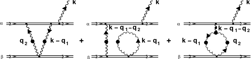
Figure 4: Some soft one-loop corrections to bremsstrahlung depicted in Fig. 1.

We consider further approximation of static color centers, i.e. we set ${\bf v}_{\beta}=0$. We substitute an expression (6.4) with partial coefficient function (6.5) into formula for radiation intensity (3.2). Delta-functions in integrands (6.4) and (6.5) in static limit results in integration measure of the form

$$\delta(v_{\alpha}\cdot k)[\delta(q_{10})\delta(q_{20})dq_{10}dq_{20}]\delta({\bf v}_{\alpha}\cdot({\bf q}_{1}+{\bf q}_{2}))d{\bf q}_{1}d{\bf q}_{2}\,d{\bf k}d\omega.$$ (6.6)

Integration over impact parameter ${\bf b}$ leads to additional delta-function in integrand

$$\int\!\!d{\bf b}\,{\rm e}^{-i({\bf q}_{1}+{\bf q}_{2})\cdot{\bf b}}=(2\pi)^{2}\delta^{(2)}(({\bf q}_{1}+{\bf q}_{2})_{\perp}).$$

This expression together with (6.6) enables us to integrate over $d{\bf q}_{2}$. Performing replacement of variable ${\bf q}_{1}\rightarrow{\bf q}$, after some algebraic transformations and regrouping the terms, we result in final expression for off-diagonal contribution to radiation energy loss of high-energy color particle $\alpha$ within static approximation

$$\left(\!-\frac{dE}{dx}\right)_{\!{\rm off-diag.}}^{\!t}=\Lambda_{1}+\Lambda_{2}.$$

Here, on the right-hand side the function $\Lambda_{1}$ is

$$\Lambda_{1}=\biggl{(}\frac{{\alpha}_{s}}{\pi}\biggr{)}^{\!3}\!C_{A}\sum\limits_{\beta=q\!,\,\bar{q}\!,\,{\rm g}}\,\Biggl{(}\frac{C_{2}^{(\alpha)}C_{2}^{(\beta)}}{d_{A}}\Biggr{)}n_{\beta}\!\sum_{\zeta=1,2}\!\int\!d{\bf k}d\omega\,\omega\,{\rm Im}(^{\ast}{\!\Delta}^{t}(k))\!\int\!d{\bf q}\,\frac{1}{({\bf q}^{2}+\mu^{2})^{2}}$$ (6.7)

$$\times\,\Biggl{[}\,\frac{({\bf e}\cdot{\bf v}_{\alpha})^{2}}{({\bf v}_{\alpha}\cdot{\bf q})^{2}}-2\,\frac{({\bf e}\cdot{\bf v}_{\alpha})}{({\bf v}_{\alpha}\cdot{\bf q})}\,{\rm Re}\,\Bigl{\{}{\rm e}^{i}(\hat{\bf k},\zeta)\,^{\ast}\Gamma^{i0\mu}(k,-q,-k+q)\!\,^{\ast}{\cal D}_{C\mu\mu^{\prime}}(k-q)v_{\alpha}^{\mu^{\prime}}\Bigr{\}}\!\Biggr{]}\delta(v_{\alpha}\cdot k),$$

and the function $\Lambda_{2}$ has a form

$$\Lambda_{2}=-\biggl{(}\frac{{\alpha}_{s}}{\pi}\biggr{)}^{\!3}\!C_{A}\!\sum\limits_{\beta=q,\,\bar{q},\,{\rm g}}\,\!\Biggl{(}\frac{C_{2}^{(\alpha)}C_{2}^{(\beta)}}{d_{A}}\Biggr{)}n_{\beta}\!\!\sum_{\zeta,\,\zeta^{\prime}=1,2}\!\int\!d{\bf k}d\omega\,\omega\,{\rm Im}(^{\ast}{\!\Delta}^{t}(k))\Bigl{\{}\!({\bf e}(\hat{\bf k},\zeta)\cdot{\bf v}_{\alpha})({\bf e}(\hat{\bf k},{\zeta}^{\prime})\cdot{\bf v}_{\alpha})\!\Bigr{\}}$$ (6.8)

$$\times\int\!d{\bf q}\,\frac{1}{({\bf q}^{2}+\mu^{2})^{2}}\,{\rm Re}\,\Bigl{\{}\,^{\ast}{\!\Delta}^{t}(k)\Bigl{(}{\rm e}^{i}(\hat{\bf k},\zeta)\,^{\ast}\tilde{\Gamma}^{i0j0}(k,q,-k,-q){\rm e}^{j}(\hat{\bf k},\zeta^{\prime})\Bigr{)}\!\Bigr{\}}\delta(v_{\alpha}\cdot k).$$

In the last expression ${}^{\ast}\tilde{\Gamma}^{i0j0}$ is an effective four-gluon vertex entered in Paper I (Eq.(I.5.6)). The diagrammatic interpretation of terms in $\Lambda_{1}$ and $\Lambda_{2}$ that easily follows from initial diagrams of Fig. 4 type, is presented in Fig. 5.

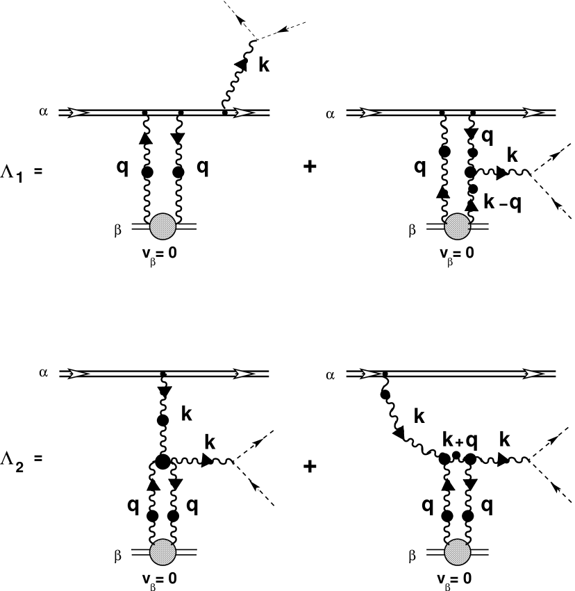
Figure 5: The diagrammatic interpretation of terms defining ‘off-diagonal’ contribution to radiation energy loss. The dotted lines denote thermal partons absorbing virtual bremsstrahlung gluons. Here, ${\bf q}$ is three-dimensional vector.

Remind that two diagrams corresponding to radiation of soft gluon prior to one-gluon exchange and after it, are determined by the first term on the right-hand side of Eq. (6.7). We depicted the second diagram in Fig. 5 only. Note also that functions $\Lambda_{1}$ and $\Lambda_{2}$ are not vanishing for plasma excitations lying off mass-shell due to delta-function in integrands.

From the form of graphs in Fig. 5 it is evident that they represent the contact double Born graphs, first considered by Zakharov [12] to ensure unitarity as was already mentioned in Introduction. However in our case propagators and vertices are effective (i.e. we take into account hard thermal loops effects) and besides additional contribution (the first diagram for $\Lambda_{2}$ in Fig. 5) connected with existence of four-gluon HTL amplitude ${}^{\ast}\Gamma_{4g}=\Gamma_{4g}+\delta\Gamma_{4g}$, appears.

Usually the contributions to radiation energy loss containing bare four-gluon vertex $\Gamma_{4g}$, are omitted for kinematical reasons [3, 4] (the absence of momentum dependence). However HTL-correction $\delta\Gamma_{4g}$ have highly nontrivial momentum dependence and therefore in advance, it is not evident that this term can give negligible small contribution, at least to region of soft transfer and soft gluon bremsstrahlung.

Let us analyze the role of contribution $\Lambda_{1}$ to the theory under consideration of bremsstrahlung. For this purpose we compare it with basic diagonal contribution (3.9) (more exactly with the first term on the right-hand side of (3.9)). Setting ${\bf v}_{\beta}=0$ we rewrite this diagonal contribution once more, considered module squared $|{\rm e}^{i}{\cal K}^{i}|^{\,2}$

$$\left(\!-\frac{dE}{dx}\right)_{\!{\rm diag.}}^{\!t}=-\biggl{(}\frac{{\alpha}_{s}}{\pi}\biggr{)}^{\!3}\!C_{A}\sum\limits_{\beta=q,\,\bar{q},\,{\rm g}}\,\Biggl{(}\frac{C_{2}^{(\alpha)}C_{2}^{(\beta)}}{d_{A}}\Biggr{)}n_{\beta}\!\sum_{\zeta=1,2}\!\int\!d{\bf k}d\omega\,\omega\,{\rm Im}(^{\ast}{\!\Delta}^{t}(k))\!\int\!d{\bf q}\,\frac{1}{({\bf q}^{2}+\mu^{2})^{2}}$$

$$\times\,\Biggl{[}\,\frac{({\bf e}\cdot{\bf v}_{\alpha})^{2}}{({\bf v}_{\alpha}\cdot{\bf q})^{2}}-2\,\frac{({\bf e}\cdot{\bf v}_{\alpha})}{({\bf v}_{\alpha}\cdot{\bf q})}\,{\rm Re}\,\Bigl{\{}{\rm e}^{i}(\hat{\bf k},\zeta)\,^{\ast}\Gamma^{i0\mu}(k,-q,-k+q)\!\,^{\ast}{\cal D}_{C\mu\mu^{\prime}}(k-q)v_{\alpha}^{\mu^{\prime}}\Bigr{\}}$$ (6.9)

$$+\,\Bigl{|}\,{\rm e}^{i}(\hat{\bf k},\zeta)\,^{\ast}\Gamma^{i0\mu}(k,-q,-k+q)\!\,^{\ast}{\cal D}_{C\mu\mu^{\prime}}(k-q)v_{\alpha}^{\mu^{\prime}}\Bigr{|}^{\,2}\Biggr{]}\delta(v_{\alpha}\cdot k+{\bf v}_{\alpha}\cdot{\bf q}).$$

If one defines the last expression on mass-shell of plasma oscillations using formula (3.10), then factors

$$\frac{1}{({\bf v}_{\alpha}\cdot{\bf q})^{2}}\equiv\frac{1}{(v_{\alpha}\cdot k)^{2}},\quad\frac{1}{({\bf v}_{\alpha}\cdot{\bf q})}\equiv-\,\frac{1}{(v_{\alpha}\cdot k)}$$

occurring in the first two terms in square brackets of integrand will not to be singular due to the fact that linear Landau damping process is absent in QGP. However for off mass-shell excitations of medium, when frequency and momentum of plasma excitations approach to “Cherenkov cone”

$$(v_{\alpha}\cdot k)\rightarrow 0,$$ (6.10)

these factors become singular, that results in divergence of the integral on the right-hand side of Eq. (6.9). From comparison of the expressions (6.9) and (6.7) we see that these singularities are exactly compensated by appropriate terms on the right-hand side of Eq. (6.7). Thus, the only complete sum of all contributions (‘diagonal’ and ‘off-diagonal’, on-shell and off-shell) to radiation energy loss of energetic parton $\alpha$ is a finite value.

The meaning of the second contribution $\Lambda_{2}$ (Eq. (6.8)) is less evident. We can only say that following reasoning in Section 9 of Paper II, this contribution to energy loss takes into account such subtle collective effect as change of chromodielectric properties of hot QCD medium induced by soft gluon self-interaction. This effect partially can be taken into account by replacement of the HTL-resummed scalar propagator ${}^{\ast}{\!\Delta}^{t}(k)$ by effective one ${}^{\ast}\tilde{\Delta}^{t}(k)$ taking into account nonlinear effects of soft gluon self-interaction in lowest order (elastic rescattering of two soft transverse gluons $gg\leftrightarrow gg$)

$${}^{\ast}\tilde{\Delta}^{\!-\!1\,t}(k)\simeq\,^{\ast}{\!\Delta}^{\!-\!1\,t}(k)-\Pi^{(1)\,t}(k).$$

Here, $\Pi^{(1)\,t}(k)$ represents the correction to transverse part of gluon self-energy in HTL-approximation, taking into account a change of dielectric properties of medium by the action of the processes of nonlinear interaction (transverse) plasma excitations among themselves. Its explicit form is similar to (II.9.5) for longitudinal part of correction.

7 Bremsstrahlung of two soft gluons

Hereafter we are concerned with higher-order processes produced soft gluon radiation. Here, we consider scattering process of color particle $\alpha$ off hard thermal parton $\beta$, when bremsstrahlung of two gluons, arises. Here, we are mainly interested in question for what typical amplitudes the soft gluon field (or, in other words, the density of soft gluon radiation) in medium, the process of bremsstrahlung of higher order will give a contribution to gluon radiation intensity of the same order as the process of bremsstrahlung discussed in previous Sections. As was mentioned in Section 6, this process is defined by the effective current

$$\tilde{J}^{(2)a}_{\mu}[Q_{0\alpha},Q_{0\beta},A^{(0)}](k)=\int\!\!K_{\mu\mu_{1}}^{aa_{1}}({\bf v}_{\alpha},{\bf v}_{\beta};{\bf b},Q_{0\alpha},Q_{0\beta}|\,k,-k_{1})A^{(0)a_{1}\mu_{1}}(k_{1})dk_{1}.$$ (7.1)

We take the coefficient function in integrand in the leading order in coupling constant, i.e.

$$K_{\mu\mu_{1}}^{aa_{1}}({\bf v}_{\alpha},{\bf v}_{\beta};{\bf b},Q_{0\alpha},Q_{0\beta}|\,k,-k_{1})\cong K_{\mu\mu_{1}}^{aa_{1}bc}({\bf v}_{\alpha},{\bf v}_{\beta};{\bf b}|\,k,-k_{1})Q_{0\alpha}^{b}Q_{0\beta}^{c}.$$ (7.2)

For the deriving of function $K_{\mu\mu_{1}}^{aa_{1}bc}({\bf v}_{\alpha},{\bf v}_{\beta};{\bf b}|\,k,-k_{1})$ we use simple and effective procedure suggested in Paper I and Paper II and extended for this case. The calculations shown that this function has a following color structure

$$K_{\mu\mu_{1}}^{aa_{1}bc}({\bf v}_{\alpha},{\bf v}_{\beta};{\bf b}|\,k,\!-k_{1})\!=\!(T^{a}T^{a_{1}})^{bc}\!K_{\mu\mu_{1}}({\bf v}_{\alpha},{\bf v}_{\beta};{\bf b}|\,k,\!-k_{1})+(T^{a_{1}}T^{a})^{bc}\!K_{\mu_{1}\mu}({\bf v}_{\alpha},{\bf v}_{\beta};{\bf b}|\,-k_{1},k).$$

The right-hand side of this expression is automatically symmetric with respect to permutation of external soft gluon legs: $k\rightleftharpoons-k_{1},\;\mu\rightleftharpoons\mu_{1},\;a\rightleftharpoons a_{1}$. The requirement of symmetry over permutation of hard lines $(\alpha\rightleftharpoons\beta,\;c\rightleftharpoons b)$ leads to additional condition for partial coefficient function $K_{\mu\mu_{1}}$:

$$K_{\mu\mu_{1}}({\bf v}_{\alpha},{\bf v}_{\beta};{\bf b}|\,k,-k_{1})=K_{\mu_{1}\mu}({\bf v}_{\beta},{\bf v}_{\alpha};-{\bf b}|\,-k_{1},k).$$

The explicit form of this function, and also graphic interpretation of different terms is given in Appendix A.

Let us substitute an expression for an effective current (7.1), (7.2) into formula (3.1) defining total energy of radiation field in single scattering. Performing average over color charges, we obtain

$$W_{2{\rm g}}({\bf b})=\biggl{(}\frac{{\alpha}_{s}}{\pi}\biggr{)}^{\!4}\Biggl{(}\frac{C_{2}^{(\alpha)}C_{2}^{(\beta)}}{d_{A}}\Biggr{)}\!\int\!d{\bf k}d\omega\,\omega\,{\rm Im}\Bigl{(}K_{\mu\mu_{1}}^{\ast aa_{1}bc}({\bf v}_{\alpha},{\bf v}_{\beta};{\bf b}|\,k,\!-k_{1})\!\,^{\ast}{\cal D}^{\mu\mu^{\prime}}_{C}(k)$$ (7.3)

$$\times K_{\mu^{\prime}\mu_{1}^{\prime}}^{aa_{1}^{\prime}b^{\prime}c^{\prime}}({\bf v}_{\alpha},{\bf v}_{\beta};{\bf b}|\,k,\!-k_{1})\Bigr{)}\langle A^{\ast(0)\,a_{1}\mu_{1}}(k_{1})A^{(0)\,a_{1}^{\prime}\mu_{1}^{\prime}}(k_{1}^{\prime})\rangle\,dk_{1}dk_{1}^{\prime}.$$

For the conditions of stationary and homogeneity of hot QCD plasma we have for correlation function of the soft boson excitations

$$\langle A^{\ast(0)\,a_{1}\mu_{1}}(k_{1})A^{(0)\,a_{1}^{\prime}\mu_{1}^{\prime}}(k_{1}^{\prime})\rangle=\delta^{a_{1}a_{1}^{\prime}}I^{\mu_{1}\mu_{1}^{\prime}}(k_{1})\delta(k_{1}-k_{1}^{\prime}).$$

One defines the spectral density $I^{\mu\nu}(k)$ in the form of an expansion

$$I^{\mu\nu}(k)=P^{\mu\nu}(k)I_{k}^{t}+\tilde{Q}^{\mu\nu}I_{k}^{l},\$$

where in turn the scalar functions $I_{k}^{t}$ and $I_{k}^{l}$ are taken in the form of the quasiparticle approximation

$$I_{k}^{t,\,l}=I_{\bf k}^{t,\,l}\delta(\omega-\omega_{\bf k}^{t,\,l})+I_{-{\bf k}}^{t,\,l}\delta(\omega+\omega_{\bf k}^{t,\,l})$$ (7.4)

$$=-\,\frac{1}{(2\pi)^{3}}\left(\frac{{\rm Z}_{t,\,l}({\bf k})}{2\omega_{\bf k}^{t,\,l}}\right)\!\Bigl{\{}N_{\bf k}^{t,\,l}\delta(\omega-\omega_{\bf k}^{t,\,l})+N_{-{\bf k}}^{t,\,l}\delta(\omega+\omega_{\bf p}^{t,\,l})\!\Bigr{\}}.$$

In the last line we pass from functions $I_{\bf k}^{t,\,l}$ to the number densities of soft plasma oscillations $N_{\bf k}^{t,\,l}$. In Eq. (7.4) the term containing delta-function $\delta(\omega+\omega_{\bf k}^{t,\,l})$ only will define contribution to energy of radiation field (7.3) connected with bremsstrahlung of two gluons. The term containing $\delta(\omega-\omega_{\bf k}^{t,\,l})$ gives contribution associated with process extending nonlinear Landau damping process (Section 3, Paper II) to the case of two hard color partons. Therefore hereafter we drop the last contribution and focus our attention on pure bremsstrahlung. Note that to take into account effects of weakly inhomogeneous and weakly non-stationary state of QGP induced by the effects of the nonlinear interaction of waves and particles, it is sufficient in the first approximation to assume that functions $N_{\bf k}^{t,\,l}$ are slowly dependent on $x=(t,{\bf x})$. In this case the functions obey proper kinetic equations, one of which will be given below.

For simplicity we restrict our consideration to bremsstrahlung of real transverse gluons. With allowance for above-mentioned in (7.3) we make following substitution

$$I^{\mu_{1}\mu_{1}^{\prime}}(k_{1})\Rightarrow\frac{1}{(2\pi)^{3}}\left(\frac{{\rm Z}_{t}({\bf k}_{1})}{2\omega_{{\bf k}_{1}}^{t}}\right)\!N_{-{\bf k}_{1}}^{t}\delta(\omega_{1}+\omega_{{\bf k}_{1}}^{t})\!\!\sum_{\zeta_{1}=1,2}{\rm e}^{\ast i_{1}}(\hat{\bf k}_{1},\zeta_{1})\,{\rm e}^{i_{1}^{\prime}}(\hat{\bf k}_{1},\zeta_{1}),$$

$$\!\,{}^{\ast}{\cal D}^{\mu\mu^{\prime}}_{C}(k)\Rightarrow\,^{\ast}{\!\Delta}^{t}(k)\!\sum_{\zeta=1,2}{\rm e}^{\ast i}(\hat{\bf k},\zeta)\,{\rm e}^{i^{\prime}}(\hat{\bf k},\zeta),\hskip 42.67912pt$$

$${\rm Im}(^{\ast}{\!\Delta}^{\!-1\,t}(k))\Rightarrow-\pi\,{\rm sign}(\omega)\left(\frac{{\rm Z}_{t}({\bf k})}{2\omega_{\bf k}^{t}}\right)\!\delta(\omega-\omega_{\bf k}^{t}).$$

Here, we have taken into account representation (3.5). Performing trivial integration over $dk_{1}^{\prime}$, $d\omega$ and $d\omega_{1}$ and replacing variable ${\bf k}_{1}\rightarrow-{\bf k}_{1}$ $(\omega_{{\bf k}_{1}}^{t}\rightarrow-\omega_{{\bf k}_{1}}^{t})$ we derive instead of (7.3)

$$(W_{2{\rm g}}({\bf b}))^{t}=\frac{1}{2(2\pi)^{2}}\,\biggl{(}\frac{{\alpha}_{s}}{\pi}\biggr{)}^{\!4}\Biggl{(}\frac{C_{2}^{(\alpha)}C_{2}^{(\beta)}}{d_{A}}\Biggr{)}\!\sum_{\zeta,\,\zeta_{1}=1,2}\!\int\!d{\bf k}d{\bf k}_{1}\,\omega_{\bf k}^{t}N_{{\bf k}_{1}}^{t}\left(\frac{{\rm Z}_{t}({\bf k})}{2\omega_{\bf k}^{t}}\right)\!\left(\frac{{\rm Z}_{t}({\bf k}_{1})}{2\omega_{{\bf k}_{1}}^{t}}\right)$$

$$\times|\,K^{aa_{1}bc\,ii_{1}}({\bf v}_{\alpha},{\bf v}_{\beta};{\bf b}|\,k,k_{1}){\rm e}^{i}(\hat{\bf k},\zeta)\,{\rm e}^{i_{1}}(\hat{\bf k}_{1},\zeta_{1})|^{\,2}_{\,{\rm on-shell}}.$$ (7.5)

Let us define an expression for gluon radiation intensity. For this purpose we write partial coefficient function $K_{\mu\mu_{1}}$ in the form of integral representation

$$K_{\mu\mu_{1}}({\bf v}_{\alpha},\!{\bf v}_{\beta};\!{\bf b}|\,k,k_{1})\!=\!\!\int\!\!{\rm e}^{i{\bf q}\cdot{\bf b}}[{\cal K}_{\mu\mu_{1}}({\bf v}_{\alpha},\!{\bf v}_{\beta}|\,k,k_{1};q)]_{q_{0}={\bf v}_{\beta}\cdot{\bf q}}\delta(\omega^{t}_{\bf k}+\omega^{t}_{{\bf k}_{1}}\!-{\bf v}_{\beta}\cdot{\bf q}-{\bf v}_{\alpha}\cdot({\bf k}+{\bf k}_{1}-{\bf q})\!)d{\bf q}.$$

The function ${\cal K}_{\mu\mu_{1}}$ is defined by integrand in Eq. (A.1). Subsequent reasoning are completely similar to those in Section 3. Performing integration over impact parameter with (3.8) and allowing for the following equalities

$$(T^{a}T^{a_{1}})^{\ast bc}(T^{a}T^{a_{1}})^{bc}=C_{A}^{2}d_{A},\quad(T^{a}T^{a_{1}})^{\ast bc}(T^{a_{1}}T^{a})^{bc}=\frac{1}{2}\,C_{A}^{2}d_{A},$$ (7.6)

we obtain expressions for intensity radiation in this case

$$\left\langle\frac{dW_{2{\rm g}}({\bf b})}{dt}\right\rangle_{\!{\bf b}}=\frac{1}{2}\,\biggl{(}\frac{{\alpha}_{s}}{\pi}\biggr{)}^{\!4}\,C_{A}^{\,2}\!\sum_{\beta=q\!,\,\bar{q}\!,\,{\rm g}}\Biggl{(}\frac{C_{2}^{(\alpha)}C_{2}^{(\beta)}}{d_{A}}\Biggr{)}\!\sum_{\zeta,\,\zeta_{1}=1,2}\!\int\!d{\bf k}d{\bf k}_{1}\,\omega_{\bf k}^{t}N_{{\bf k}_{1}}^{t}\left(\frac{{\rm Z}_{t}({\bf k})}{2\omega_{\bf k}^{t}}\right)\!\left(\frac{{\rm Z}_{t}({\bf k}_{1})}{2\omega_{{\bf k}_{1}}^{t}}\right)$$

$$\times\Biggl{(}\int\!{\bf p}_{\beta}^{2}f_{|{\bf p}_{\beta}|}\,\frac{d|{\bf p}_{\beta}|}{2\pi^{2}}\Biggr{)}\int\!\frac{d\Omega_{{\bf v}_{\beta}}}{4\pi}\!\int\!d{\bf q}\,\delta(\omega^{t}_{\bf k}+\omega^{t}_{{\bf k}_{1}}-{\bf v}_{\beta}\cdot{\bf q}-{\bf v}_{\alpha}\cdot({\bf k}+{\bf k}_{1}-{\bf q}))$$ (7.7)

$$\times\biggl{\{}|\,{\cal K}^{ii_{1}}({\bf v}_{\alpha},{\bf v}_{\beta}|\,k,k_{1},q){\rm e}^{i}(\hat{\bf k},\zeta){\rm e}^{i_{1}}(\hat{\bf k}_{1},\zeta_{1})|^{\,2}+|\,{\cal K}^{i_{1}i}({\bf v}_{\alpha},{\bf v}_{\beta}|\,k_{1},k,q){\rm e}^{i_{1}}(\hat{\bf k}_{1},\zeta_{1}){\rm e}^{i}(\hat{\bf k},\zeta)|^{\,2}$$

$$+{\rm Re}\Bigl{[}\Bigl{(}\,{\cal K}^{ii_{1}}({\bf v}_{\alpha},{\bf v}_{\beta}|\,k,k_{1},q){\rm e}^{i}(\hat{\bf k},\zeta){\rm e}^{i_{1}}(\hat{\bf k}_{1},\zeta_{1})\Bigr{)}^{\!{\ast}}\!\Bigl{(}{\cal K}^{i_{1}i}({\bf v}_{\alpha},{\bf v}_{\beta}|\,k_{1},k,q){\rm e}^{i_{1}}(\hat{\bf k}_{1},\zeta_{1}){\rm e}^{i}(\hat{\bf k},\zeta)\Bigr{)}\Bigr{]}\!\biggr{\}}_{\!q_{0}={\bf v}_{\beta}\cdot{\bf q}}.$$

Here, the integrand can be made completely symmetric over permutation ${\bf k}\rightleftharpoons{\bf k}_{1}$ if we replace: $\omega_{\bf k}^{t}N_{{\bf k}_{1}}^{t}\rightarrow(\omega_{\bf k}^{t}N_{{\bf k}_{1}}^{t}+\omega_{{\bf k}_{1}}^{t}N_{\bf k}^{t})/2$. Similar to (3.3) one can define probability of two-gluon bremsstrahlung ${\it w}_{{\bf p}_{\alpha},\,{\bf p}_{\beta}}({\bf k},{\bf k}_{1};{\bf q})$ if radiation intensity is written as follows

$$\left\langle\frac{dW_{2{\rm g}}({\bf b})}{dt}\right\rangle_{\!{\bf b}}\!=\!\int\!\omega_{\bf k}^{t}N_{{\bf k}_{1}}^{t}{\it w}_{{\bf p}_{\alpha},\,{\bf p}_{\beta}}({\bf k},{\bf k}_{1};{\bf q})\,\frac{f_{{\bf p}_{\beta}}d{\bf p}_{\beta}}{(2\pi)^{3}}\,\frac{d{\bf k}d{{\bf k}_{1}}d{\bf q}}{(2\pi)^{9}}\,\delta(\omega^{t}_{\bf k}+\omega^{t}_{{\bf k}_{1}}-{\bf v}_{\beta}\cdot{\bf q}-{\bf v}_{\alpha}\cdot({\bf k}+{\bf k}_{1}-{\bf q})).$$

Comparing the last expression with (7.7) it is not difficult to obtain an explicit form of required probability.

In limit static case of target $({\bf v}_{\beta}=0)$ an expression (7.7) defines ‘net’ energy loss of projectile $\alpha$. Setting ${\bf v}_{\beta}=0$ in Eq. (A.1) we obtain considerable simpler expression for partial coefficient function ${\cal K}^{ii_{1}}$ entering into integrand (7.7)

$${\cal K}^{ii_{1}}({\bf v}_{\alpha},0|\,k,k_{1},q)=\frac{1}{{\bf q}^{2}+\mu_{D}^{2}}\,\Biggl{[}\,\frac{v_{\alpha}^{i}v_{\alpha}^{i_{1}}}{(v_{\alpha}\cdot q)(v_{\alpha}\cdot(q-k_{1}))}$$

$$+\,\frac{v_{\alpha}^{i}}{v_{\alpha}\cdot(q-k_{1})}\,\,v_{\alpha}^{\nu}\,{}^{\ast}{\cal D}_{C\nu\nu^{\prime}}\!(q-k_{1})\,^{\ast}\Gamma^{\nu^{\prime}i_{1}0}(q-k_{1},k_{1},-q)$$ (7.8)

$$+\,^{\ast}\Gamma^{i\nu\lambda}(k,k_{1}-q,-k-k_{1}+q)\!\,^{\ast}{\cal D}_{C\nu\nu^{\prime}}\!(q-k_{1})\,^{\ast}\Gamma^{\nu^{\prime}i_{1}0}(q-k_{1},k_{1},-q)\!\,^{\ast}{\cal D}_{C\lambda\lambda^{\prime}}\!(k+k_{1}-q)v_{\alpha}^{\lambda^{\prime}}$$

$$+\,^{\ast}\Gamma^{ii_{1}\lambda}(k,k_{1},-k-k_{1})\!\,^{\ast}{\cal D}_{C\lambda\lambda^{\prime}}\!(k+k_{1})\biggl{\{}\,\frac{v_{\alpha}^{\lambda^{\prime}}}{v_{\alpha}\cdot q}+\,^{\ast}\Gamma^{\lambda^{\prime}0\nu}(k+k_{1},-q,-k-k_{1}+q)\!\,^{\ast}{\cal D}_{C\nu\nu^{\prime}}\!(k+k_{1}-q)v_{\alpha}^{\nu^{\prime}}\biggr{\}}$$

$$-\,^{\ast}\Gamma^{i\nu 0i_{1}}(k,-k-k_{1}+q,-q,k_{1})\!\,^{\ast}{\cal D}_{C\nu\nu^{\prime}}\!(k+k_{1}-q)v_{\alpha}^{\nu^{\prime}}\Biggr{]}_{\!q_{0}=0}.$$

Diagrammatic interpretation of different terms is presented in Fig. 6.

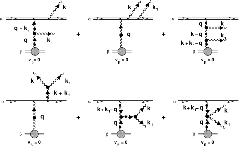
Figure 6: The processes of bremsstrahlung of two soft gluons in static potential model.

As in previous cases, here we have not presented diagrams of the bremsstrahlung of two gluons a prior to one-gluon exchange. In semiclassical approximation all these process are automatically taken into account on the right-hand side of Eq. (7.8).

The expression (7.7) in region of soft momentum transfer $(|{\bf q}|\leq gT)$ is distinct in value order from the expression (3.9) associated with bremsstrahlung of one soft gluon by factor

$$\alpha_{s}\!\int\!d{\bf k}_{1}\left(\frac{{\rm Z}_{t}({\bf k}_{1})}{2\omega_{{\bf k}_{1}}^{t}}\right)\frac{1}{(v_{\alpha}\cdot(k-q))^{2}}\,N^{t}_{{\bf k}_{1}}\sim\alpha_{s}(gT)^{3}\frac{1}{gT}\,\frac{1}{(gT)^{2}}\,N^{t}_{{\bf k}_{1}}\sim\alpha_{s}N^{t}_{{\bf k}_{1}}.$$ (7.9)

Here, we take into account that for soft gluon $\omega_{\bf k}^{t},\,|{\bf k}|\sim gT$. For low density of soft gluon radiation in medium, corresponding to the level of thermal fluctuations at soft scale $gT$ (Eq. (I.6.5)), when

$$|A_{\mu}(X)|\sim\sqrt{g}T,\quad N_{\bf k}^{t}\sim\frac{1}{g},$$ (7.10)

from estimation (7.9) it follows that bremsstrahlung of two soft gluons is suppressed by more power $g$ in comparison with bremsstrahlung of one soft gluon.

In opposite case for the field as strong as allowed (Eq. (I.6.4))

$$|A_{\mu}(X)|\sim T,\quad N_{\bf k}^{t}\sim\frac{1}{g^{2}},$$ (7.11)

we see from (7.9) that considered process (and also generally speaking all other higher processes of bremsstrahlung of arbitrary number of soft gluons) becomes of the same order in coupling constant. Here, the problem of resummation of all relevant contributions to soft gluon radiation intensity arises. As mentioned above in the case of slowly inhomogeneous and nonstationarity QGP, an explicit form of the number density $N_{\bf k}^{t}$ is determined by solution of kinetic equation of Boltzmann type

$$\frac{\partial N_{\bf k}^{t}}{\partial t}+{\bf v}_{\bf k}^{t}\cdot\frac{\partial N_{\bf k}^{t}}{\partial{\bf x}}=-N_{\bf k}^{t}\Gamma_{\rm d}[N_{\bf k}^{t}]+(1+N_{\bf k}^{t})\Gamma_{\rm i}[N_{\bf k}^{t}],$$ (7.12)

where ${\bf v}_{\bf k}^{t}=\partial\omega_{\bf k}^{t}/\partial{\bf k}$ is a group velocity of the transverse oscillations. The functional dependence is denoted by argument of a function in square brackets.

A generalized decay rate $\Gamma_{\rm d}$ and regenerating rate $\Gamma_{\rm i}$ are written in the form of functional expansion in powers of the number density $N_{\bf k}^{t}$

$$\Gamma_{\rm d}[N_{\bf k}^{t}]=\sum_{n=0}^{\infty}\Gamma_{\rm d}^{(n)}[N_{\bf k}^{l}],\;\;\Gamma_{\rm i}[N_{\bf k}^{t}]=\sum_{n=0}^{\infty}\Gamma_{\rm i}^{(n)}[N_{\bf k}^{t}].$$ (7.13)

Here,

$$\Gamma_{\rm d}^{(n)}[N_{\bf k}^{t}]=\sum\limits_{\beta=q\!,\,\bar{q}\!,\,{\rm g}}\int\!\frac{d{\bf p}_{\beta}}{(2\pi)^{3}}\,f_{{\bf p}_{\beta}-\,{\bf q}}\!\int\!{\it w}_{{\bf p}_{\alpha},\,{\bf p}_{\beta}}({\bf k},{\bf k}_{1},\ldots,{\bf k}_{n};\,{\bf q})N_{{\bf k}_{1}}^{t}\ldots N_{{\bf k}_{n}}^{t}$$

$$\times\,\delta\Bigl{(}E_{{\bf p}_{\alpha}}+E_{{\bf p}_{\beta}}-E_{{\bf p}_{\alpha}+{\bf q}-{\bf k}_{\rm tot}}-E_{{\bf p}_{\beta}-{\bf q}}-{\cal E}_{\rm tot}\Bigr{)}\,\frac{d{\bf q}}{(2\pi)^{3}}\prod\limits_{i=1}^{n}\frac{d{\bf k}_{i}}{(2\pi)^{3}}\,,$$

$$\Gamma_{\rm d}^{(n)}[N_{\bf k}^{t}]=\sum\limits_{\beta=q\!,\,\bar{q}\!,\,{\rm g}}\int\!\frac{d{\bf p}_{\beta}}{(2\pi)^{3}}\,f_{{\bf p}_{\beta}}\!\int\!{\it w}_{{\bf p}_{\alpha},\,{\bf p}_{\beta}}({\bf k},{\bf k}_{1},\ldots,{\bf k}_{n};\,{\bf q})(1+N_{{\bf k}_{1}}^{t})\ldots(1+N_{{\bf k}_{n}}^{t})$$

$$\times\,\delta\Bigl{(}E_{{\bf p}_{\alpha}}+E_{{\bf p}_{\beta}}-E_{{\bf p}_{\alpha}+{\bf q}-{\bf k}_{\rm tot}}-E_{{\bf p}_{\beta}-{\bf q}}-{\cal E}_{\rm tot}\Bigr{)}\,\frac{d{\bf q}}{(2\pi)^{3}}\prod\limits_{i=1}^{n}\frac{d{\bf k}_{i}}{(2\pi)^{3}}\,,$$

where

$${\cal E}_{\rm tot}\equiv\omega_{\bf k}^{t}+\sum\limits_{i=1}^{n}\omega_{{\bf k}_{i}}^{t},\quad{\bf k}_{\rm tot}\equiv{\bf k}+\sum\limits_{i=1}^{n}{\bf k}_{i},$$

and ${\it w}_{{\bf p}_{\alpha},\,{\bf p}_{\beta}}({\bf k},{\bf k}_{1},\ldots,{\bf k}_{n};\,{\bf q})$ is a probability of bremsstrahlung of $(n+1)$ soft gluons. The particular expressions for the cases $n=0$ and $n=1$ are given by Eqs. (3.12) and (7.7), correspondingly. Note that, the expressions for generalized decay and regenerating rates were simplified in the sense that a contributions of more complicated ‘mixed’ type being combination of the scattering processes of Compton type and pure bremsstrahlung, are not taken into account.

In conditions of (7.10) each subsequent term in the functional expansions (7.1) is suppressed by more power $g$, and here we can only restrict ourselves to the first leading term. By virtue of the fact that $\Gamma_{\rm d,\,i}^{(0)}$ are not $N_{\bf k}^{t}$ dependent, the Boltzmann equation (7.12) will be linear with respect to the number density. For highly excited system, Eq. (7.11), all terms in the expansions (7.13) become of the same order in magnitude, and kinetic equation (7.12) is completely nonlinear one.

8 Bremsstrahlung of two soft gluons (continuation)

Let us analyze the expression for radiation intensity (7.7) in more detail. For this purpose we introduce new partial coefficient functions

$${\cal K}^{(S)ii_{1}}({\bf v}_{\alpha},{\bf v}_{\beta}|\,k,k_{1},q)\equiv\frac{1}{2}\,\biggl{(}{\cal K}^{ii_{1}}({\bf v}_{\alpha},{\bf v}_{\beta}|\,k,k_{1},q)+{\cal K}^{i_{1}i}({\bf v}_{\alpha},{\bf v}_{\beta}|\,k_{1},k,q)\biggr{)},$$ (8.1)

$${\cal K}^{(A)ii_{1}}({\bf v}_{\alpha},{\bf v}_{\beta}|\,k,k_{1},q)\equiv\frac{1}{2}\,\biggl{(}{\cal K}^{ii_{1}}({\bf v}_{\alpha},{\bf v}_{\beta}|\,k,k_{1},q)-{\cal K}^{i_{1}i}({\bf v}_{\alpha},{\bf v}_{\beta}|\,k_{1},k,q)\biggr{)},\hskip 22.76228pt$$

the former of which is symmetric function and the second one is antisymmetric relative to permutation: $k\rightleftharpoons k_{1},\,i\rightleftharpoons i_{1}$. In terms of the functions (8.1) an expression within curly brackets in integrand of equation (7.7) is rewritten in the form (for brevity we suppress arguments of functions)

$$|\,{\cal K}^{ii_{1}}{\rm e}^{i}{\rm e}^{i_{1}}|^{\,2}+|\,{\cal K}^{i_{1}i}{\rm e}^{i_{1}}{\rm e}^{i}|^{\,2}+{\rm Re}\Bigl{[}\Bigl{(}\,{\cal K}^{ii_{1}}{\rm e}^{i}{\rm e}^{i_{1}}\Bigr{)}^{\!{\ast}}\!\Bigl{(}{\cal K}^{i_{1}i}{\rm e}^{i_{1}}{\rm e}^{i}\Bigr{)}\Bigr{]}=3|\,{\cal K}^{(S)ii_{1}}{\rm e}^{i}{\rm e}^{i_{1}}|^{\,2}+|\,{\cal K}^{(A)i_{1}i}{\rm e}^{i_{1}}{\rm e}^{i}|^{\,2}.$$

As we see from the right-hand side of this expression an interference term is vanish when start using new functions, and thus the probability of bremsstrahlung of two gluons decomposes into two completely independent parts. This points to the fact that the process can proceed through two physically independent channels determined by parity of final state of two gluon‘s system with respect to permutation of external soft-gluon legs. The functions ${\cal K}^{(S)ii_{1}}{\rm e}^{i}{\rm e}^{i_{1}}_{1}$ and ${\cal K}^{(A)ii_{1}}{\rm e}^{i}{\rm e}^{i_{1}}_{1}$ define a matrix elements of bremsstrahlung of two gluons being in even state and in odd state, correspondingly.

Note that going to functions (8.1) having more clear physical meaning can be already performed at the level of initial effective current (7.1) (with approximation (7.2) for integrand) by rewriting coefficient function $K_{\mu\mu_{1}}^{aa_{1}bc}$ in the form

$$K_{\mu\mu_{1}}^{aa_{1}bc}({\bf v}_{\alpha},\!{\bf v}_{\beta};\!{\bf b}|\,k,\!-k_{1})\!=\!\{T^{a}\!,T^{a_{1}}\}^{\!bc}K^{(S)}_{\mu\mu_{1}}({\bf v}_{\alpha},\!{\bf v}_{\beta};\!{\bf b}|\,k,\!-k_{1})+[T^{a_{1}}\!,T^{a}]^{bc}K^{(A)}_{\mu_{1}\mu}({\bf v}_{\alpha},\!{\bf v}_{\beta};{\bf b}|\,-k_{1},k),$$

where

$$K^{(S\!,\,A)}_{\mu\mu_{1}}({\bf v}_{\alpha},{\bf v}_{\beta};{\bf b}|\,k,\!-k_{1})\equiv\frac{1}{2}\,\biggl{(}K_{\mu\mu_{1}}({\bf v}_{\alpha},{\bf v}_{\beta};{\bf b}|\,k,\!-k_{1})\pm K_{\mu_{1}\mu}({\bf v}_{\alpha},{\bf v}_{\beta};{\bf b}|\,\!-k_{1},\!k)\biggr{)}$$

are symmetrized and anti-symmetrized partial coefficient functions in ‘impact parameter representation’. A purely “Abelian” part of the bremsstrahlung of two gluons is defined by a term $\{T^{a}\!,T^{a_{1}}\}^{\!bc}K^{(S)}_{\mu\mu_{1}}({\bf v}_{\alpha},\!{\bf v}_{\beta};\!{\bf b}|\,k,\!-k_{1})$.

One would expect that after separation of ‘elastic’ factor from ${\cal K}_{\mu\mu_{1}}({\bf v}_{\alpha},{\bf v}_{\beta}|\,k,k_{1},q)$ (i.e. the factor defining a scattering process without radiation) at least symmetric function ${\cal K}^{(S)}_{\mu\mu_{1}}({\bf v}_{\alpha},{\bf v}_{\beta}|\,k,k_{1},q)$ can be presented in factorized form – in the form of product of two functions separately depending on momenta $k$ and $k_{1}$. Such factorization takes place in the case of QED interaction in the semiclassical limit [77]. Further for simplicity we restrict our consideration to static case ${\bf v}_{\beta}=0\,(q_{0}=0)$. Making use explicit expression (7.8), we write out a matrix element ${\cal K}^{(S)ii_{1}}{\rm e}^{i}{\rm e}^{i_{1}}_{1}$ separating out ‘elastic’ factor

$${\cal K}^{(S)ii_{\!1}}\!({\bf v}_{\alpha},0|\,k,k_{1},q){\rm e}^{i}(\hat{\bf k},\zeta){\rm e}^{i_{1}}(\hat{\bf k}_{1},\zeta_{1})=\frac{1}{2({\bf q}^{2}+\mu_{D}^{2})}\,{\cal M}^{(S)ii_{\!1}}({\bf v}_{\alpha},0|\,k,k_{1},q){\rm e}^{i}(\hat{\bf k},\zeta){\rm e}^{i_{1}}(\hat{\bf k}_{1},\zeta_{1}),$$

where

$${\cal M}^{(S)ii_{1}}({\bf v}_{\alpha},0|\,k,k_{1},q)=\,\frac{v_{\alpha}^{i}v_{\alpha}^{i_{1}}}{(v_{\alpha}\cdot k)(v_{\alpha}\cdot k_{1})}$$ (8.2)

$$+\left\{\frac{v_{\alpha}^{i}}{(v_{\alpha}\cdot k)}\,\,v_{\alpha}^{\nu}\,{}^{\ast}{\cal D}_{C\nu\nu^{\prime}}\!(q-k_{1})\,^{\ast}\Gamma^{\nu^{\prime}i_{1}0}(q-k_{1},k_{1},-q)+(k\rightleftharpoons k_{1},\,i\rightleftharpoons i_{1})\right\}$$

$$+\,\biggl{[}\,^{\ast}\Gamma^{i\nu\lambda}(k,k_{1}-q,-k-k_{1}+q)\!\,^{\ast}{\cal D}_{C\nu\nu^{\prime}}\!(q-k_{1})\,^{\ast}\Gamma^{\nu^{\prime}i_{1}0}(q-k_{1},k_{1},-q)\!\,^{\ast}{\cal D}_{C\lambda\lambda^{\prime}}\!(k+k_{1}-q)v_{\alpha}^{\lambda^{\prime}}$$

$$+\,(k\rightleftharpoons k_{1},\,i\rightleftharpoons i_{1})\biggr{]}$$

$$+\left(\,{}^{\ast}\Gamma^{ii_{1}\lambda}(k,k_{1},-k-k_{1})+\,^{\ast}\Gamma^{i_{1}i\lambda}(k_{1},k,-k-k_{1})\right)\!\,^{\ast}{\cal D}_{C\lambda\lambda^{\prime}}\!(k+k_{1})$$

$$\times\!\left(\,\frac{v_{\alpha}^{\lambda^{\prime}}}{(v_{\alpha}\cdot q)}+\,^{\ast}\Gamma^{\lambda^{\prime}0\nu}(k+k_{1},-q,-k-k_{1}+q)\!\,^{\ast}{\cal D}_{C\nu\nu^{\prime}}\!(k+k_{1}-q)v_{\alpha}^{\nu^{\prime}}\right)$$

$$-\,\biggl{\{}\!\,^{\ast}\Gamma^{i\nu 0i_{1}}(k,-k-k_{1}+q,-q,k_{1})+\,^{\ast}\Gamma^{i_{1}\nu 0i}(k_{1},-k-k_{1}+q,-q,k)\biggr{\}}\!\,^{\ast}{\cal D}_{C\nu\nu^{\prime}}\!(k+k_{1}-q)v_{\alpha}^{\nu^{\prime}}.$$

On writing this expression we use energy-momentum conservation law in the semiclassical limit: $v_{\alpha}\cdot(k+k_{1}-q)=0$. The fourth term on the right-hand side of Eq. (8.2) vanishes owing to property

$$\,{}^{\ast}\Gamma^{ii_{1}\lambda}(k,k_{1},-k-k_{1})=-\,^{\ast}\Gamma^{i_{1}i\lambda}(k_{1},k,-k-k_{1}).$$

The last term on the right-hand side of Eq. (8.2) contains contributions associated with effective four-gluon vertex $\,{}^{\ast}\Gamma_{4g}=\Gamma_{4g}+\delta\Gamma_{4g}$. If we drop four-gluon HTL-correction $\delta\Gamma_{4g}$, then this term assumes the following form in the static limit

$$-2\delta^{ii_{1}}\,\frac{(k+k_{1}-q)^{2}}{({\bf k}+{\bf k}_{1}-{\bf q})^{2}}\,\,^{\ast}{\!\Delta}^{l}(k+k_{1}-q).$$

Thus a term containing bare four-gluon vertices $\Gamma_{4g}$ will be proportional to longitudinal part of HTL-resummed gluon propagator.

From Eq. (8.2) we see that even if we drop the contributions containing longitudinal part of gluon propagators (in particular contributions contained four-gluon vertex $\Gamma_{4g}$) and neglect by HTL correction $\delta\Gamma_{4g}$, then we still can’t present symmetrized function ${\cal M}^{(S)ii_{1}}({\bf v}_{\alpha},0|\,k,k_{1},q)$ in the factorized form

$${\cal M}^{(S)ii_{1}}({\bf v}_{\alpha},0|\,k,k_{1},q)={\cal M}^{i}({\bf v}_{\alpha},0|\,k,q){\cal M}^{i_{1}}({\bf v}_{\alpha},0|\,k_{1},q),$$ (8.3)

where

$${\cal M}^{i}({\bf v}_{\alpha},0|\,k,q)=\frac{v_{\alpha}^{i}}{(v_{\alpha}\cdot k)}+v_{\alpha}^{\nu}\,{}^{\ast}{\cal D}_{C\nu\nu^{\prime}}\!(q-k)\,^{\ast}\Gamma^{\nu^{\prime}i0}(q-k,k,-q)$$

is function on which the probability of bremsstrahlung of soft transverse gluon (Eqs. (4.1), (4.3)) is determined. Let us suppose that an equality (8.3) is true for the time being and even moreover a similar factorization is true for radiation process of arbitrary number of soft gluons, i.e.

$${\cal M}^{(S)ii_{1}\dots i_{n}}({\bf v}_{\alpha},0|\,k,k_{1},\dots,q)\!=\!{\cal M}^{i}({\bf v}_{\alpha},0|\,k,q){\cal M}^{i_{1}}({\bf v}_{\alpha},0|\,k_{1},q)\ldots{\cal M}^{i_{n}}({\bf v}_{\alpha},0|\,k_{n},q),$$ (8.4)

$$n=1,2,\dots.$$

In this case it is easy to show that an expression for total energy loss of high-energy parton induced by bremsstrahlung of arbitrary number of soft gluons can be presented in highly compact form

$$\left\langle\frac{dW_{\rm tot}^{(S)}({\bf b})}{dt}\right\rangle_{\!\!{\bf b}}=\sum\limits_{n=1}^{\infty}\left\langle\frac{dW_{n{\rm g}}^{(S)}({\bf b})}{dt}\right\rangle_{\!\!{\bf b}}$$ (8.5)

$$\cong{\alpha}_{s}^{2}\!\sum_{\beta=q,\,\bar{q},\,{\rm g}}\Biggl{(}\frac{C_{2}^{(\alpha)}C_{2}^{(\beta)}}{d_{A}}\Biggr{)}n_{\beta}\!\int\!\frac{d{\bf q}}{({\bf q}^{2}+\mu_{D}^{2})^{2}}\int\!\frac{d\tau}{2\pi}\,{\rm e}^{i({\bf v}_{\alpha}\cdot{\bf q})\tau}$$

$$\times\Biggl{\{}\frac{\alpha_{s}}{\pi^{2}}\,C_{A}\!\!\sum_{\zeta=1,2}\!\int\!d{\bf k}\,{\rm e}^{i(v_{\alpha}\cdot k)\tau}\omega_{\bf k}^{t}\!\left(\frac{{\rm Z}_{t}({\bf k})}{2\omega_{\bf k}^{t}}\right)\!|\,{\cal M}^{i}({\bf v}_{\alpha},0|\,k,q){\rm e}^{i}(\hat{\bf k},\zeta)|^{\,2}\Biggr{\}}_{\!q_{0}=0}$$

$$\times\exp\Biggl{[}\frac{3\alpha_{s}}{2\pi^{2}}\,C_{A}\!\!\sum_{\zeta_{1}=1,2}\!\int\!d{\bf k}_{1}\,{\rm e}^{i(v_{\alpha}\cdot k_{1})\tau}N_{{\bf k}_{1}}^{t}\!\left(\frac{{\rm Z}_{t}({\bf k}_{1})}{2\omega_{{\bf k}_{1}}^{t}}\right)\!|\,{\cal M}^{i_{1}}({\bf v}_{\alpha},0|\,k_{1},q){\rm e}^{i_{1}}(\hat{\bf k}_{1},\zeta_{1})|^{\,2}_{\,q_{0}=0}\Biggr{]}.$$

In the second line of this equation we separate out an ‘elastic’ part. In the deriving of Eq. (8.5) we making use the fact that the momentum-energy constraint can be factorized through the Fourier representation

$$\delta(v_{\alpha}\cdot(k+k_{1}+\ldots+k_{n}-q))|_{q_{0}=0}=\int\limits^{+\infty}_{-\infty}\frac{d\tau}{2\pi}\,{\rm e}^{i({\bf v}_{\alpha}\cdot{\bf q})\tau}{\rm e}^{i(v_{\alpha}\cdot k)\tau}\prod\limits_{l=1}^{n}\!{\rm e}^{i(v_{\alpha}\cdot k_{l})\tau}.$$

At the soft momentum scale for low-excited QGP (an estimation (7.10)) exponential factor on the right-hand side of Eq. (8.5) is of order one and thus the energy loss in the leading order is defined by bremsstrahlung of one gluon. In opposite case high-excited QGP (an estimation (7.11)) argument of exponential function is not perturbatively small, and therefore in this case we can expect essential increase of radiation energy loss.

Unfortunately for QCD interaction even within semiclassical approximation and for “Abelian” part of soft gluon emission factorizations (8.3), (8.4) don‘t take place, and therefore a simple and descriptive formula (8.5) for energy loss here is not correct. This points to the fact that multiple soft gluon radiation is not in general Poisson process and in this way the Poisson approximation for multiple soft gluon radiation used in a number of works (e.g. [78, 41, 43]), is not correct.

Let us derive an expression for symmetrized part of matrix element of two soft-gluon bremsstrahlung ${\cal K}^{(S)ii_{1}}({\bf v}_{\alpha},0|\,k,k_{1},q){\rm e}^{i}(\hat{\bf k},\zeta){\rm e}^{i_{1}}(\hat{\bf k}_{1},\zeta_{1})$ in high-frequency and small-angle approximations, similar to expression ${\cal M}^{i}({\bf v}_{\alpha},0|\,k,q){\rm e}^{i}(\hat{\bf k},\zeta)$ defined in Section 4, i.e. in conditions when we can neglect by HTL-corrections to vertices of interaction and longitudinal part of gluon propagators on the right-hand side of Eq. (8.2).

The Coulomb factor in this approximation reads

$$\frac{1}{{\bf q}^{2}+\mu_{D}^{2}}\simeq\frac{1}{{\bf q}_{\perp}^{\,2}+\mu_{D}^{2}+\displaystyle\frac{1}{v_{\alpha}^{2}}\left(\frac{1}{\tau_{f}}+\frac{1}{\tau_{\!1f}}\right)^{2}}\,,$$

where

$${\tau}_{f}\equiv\frac{2\omega}{({\bf k}_{\perp}^{2}+m_{g}^{2}+x^{2}M^{2})},\quad{\tau}_{\!1f}\equiv\frac{2\omega_{1}}{({\bf k}_{1\perp}^{2}+m_{g}^{2}+x_{1}^{2}M^{2})},\quad x=\frac{\omega}{E},\,\,x_{1}=\frac{\omega_{1}}{E},$$ (8.6)

are formation times. Furthermore the functions $({\bf e}\cdot{\bf v}_{\alpha})/(v_{\alpha}\cdot k)$ and $({\bf e}_{1}\cdot{\bf v}_{\alpha})/(v_{\alpha}\cdot k_{1})$ entering into the first term on the right-hand side of Eq. (8.2) is approximated by an expression of (4.7) type. The second term is approximated by a similar way as it was made for term (4.9), where except usual requirements in the form

$$\omega\tau_{f}\gg 1,\quad\omega_{1}\tau_{1f}\gg 1$$

it is necessary to consider that inequalities

$$\omega_{1}\tau_{f}\gg 1,\quad\omega\tau_{1f}\gg 1$$

are also fulfilled. Uniquely, the approximation of the transverse scalar propagator $\,{}^{\ast}{\!\Delta}^{t}(q-k)$ requires more accuracy. Instead of approximation (4.10) in this case we will have

$$({\bf k}-{\bf q})^{2}\simeq({\bf k}-{\bf q})^{2}_{\perp}+\frac{1}{v_{\alpha}^{2}}\left(\omega+\frac{1}{\tau_{1f}}\right)^{2}\simeq{\bf k}^{2}+({\bf k}-{\bf q})^{2}_{\perp}+m_{g}^{2}+x^{2}M^{2}+\frac{2}{v_{\alpha}^{2}}\,\frac{\omega}{\tau_{1f}}\,,$$ (8.7)

and hence expression (4.11) must be replaced by

$${}^{\ast}\!\Delta^{t}(q-k)\simeq-\frac{1}{({\bf k}-{\bf q})^{2}_{\perp}+m_{g}^{2}+x^{2}M^{2}+\biggl{(}\displaystyle\frac{x}{x_{1}}\biggr{)}({\bf k}_{1\perp}^{2}+m_{g}^{2}+x_{1}^{2}M^{2})}\,.$$ (8.8)

The third term on the right-hand side of Eq. (8.2) is more complicated for analysis. Neglecting by HTL-correction to bare three-gluon vertices and longitudinal part of gluon propagators, contracting with ${\rm e}^{i}(\hat{\bf k},\zeta){\rm e}^{i_{1}}(\hat{\bf k}_{1},\zeta_{1})$ and taking into account the equalities ${\bf e}\cdot{\bf k}={\bf e}_{1}\cdot{\bf k}_{1}=0$, we have an exact expression initial for analysis

$$2\omega_{1}\,^{\ast}\!\Delta^{t}(q-k_{1})\,^{\ast}\!\Delta^{t}(k+k_{1}-q)\Biggl{\{}-2({\bf e}\cdot({\bf k}_{1}-{\bf q}))({\bf e}_{1}\cdot{\bf v}_{\alpha})+({\bf e}_{1}\cdot(2{\bf k}-{\bf q}))({\bf e}\cdot{\bf v}_{\alpha})$$

$$-\,({\bf v}_{\alpha}\cdot({\bf k}-{\bf k}_{1}+{\bf q}))({\bf e}\cdot{\bf e}_{1})+\frac{\omega+\omega_{1}}{({\bf k}+{\bf k}_{1}-{\bf q})^{2}}\,\!\biggl{[}\Bigl{(}\,{\bf k}^{2}-({\bf k}_{1}-{\bf q})^{2}\Bigr{)}({\bf e}\cdot{\bf e}_{1})-({\bf e}\cdot({\bf k}_{1}-{\bf q}))({\bf e}_{1}\cdot{\bf q})\biggr{]}$$

$$+\,v_{\alpha}^{2}\frac{({\bf e}_{1}\cdot{\bf q})}{({\bf k}_{1}-{\bf q})^{2}}\biggl{[}({\bf e}\cdot{\bf v}_{\alpha})((2{\bf k}+{\bf k}_{1}-{\bf q})\cdot({\bf k}_{1}-{\bf q}))-(\omega+\omega_{1})({\bf e}\cdot({\bf k}_{1}-{\bf q}))\biggl{(}1-\frac{{\bf k}^{2}}{({\bf k}+{\bf k}_{1}-{\bf q})^{2}}\biggr{)}\biggr{]}\!\Biggr{\}}.$$

In the small-angle approximation next expressions hold

$${\bf e}\cdot{\bf k}\simeq{\bf e}_{\perp}\cdot\Bigl{(}{\bf k}_{1}-\frac{x_{1}}{x}{\bf k}_{\perp}\Bigr{)},\quad{\bf e}_{1}\cdot{\bf k}\simeq{\bf e}_{1\perp}\cdot\Bigl{(}{\bf k}-\frac{x}{x_{1}}{\bf k}_{1\perp}\Bigr{)},$$

$${\bf e}\cdot{\bf q}\simeq{\bf e}_{\perp}\cdot{\bf q}_{\perp},\quad{\bf e}_{1}\cdot{\bf q}\simeq{\bf e}_{1\perp}\cdot{\bf q}_{\perp},\quad{\bf e}\cdot{\bf e}_{1}\simeq{\bf e}_{\perp}\cdot{\bf e}_{1\perp},$$

$$(2{\bf k}+{\bf k}_{1}-{\bf q})\cdot({\bf k}_{1}-{\bf q})\simeq\omega_{1}(2\omega+\omega_{1}),$$

etc. Let us consider in more detail an approximation of coefficient before scalar product $({\bf e}\cdot{\bf e}_{1})$, that is equals to

$$-\,{\bf v}_{\alpha}\cdot({\bf k}-{\bf k}_{1}+{\bf q})+\frac{\omega+\omega_{1}}{({\bf k}+{\bf k}_{1}-{\bf q})^{2}}\,\Bigl{(}\,{\bf k}^{2}-({\bf k}_{1}-{\bf q})^{2}\Bigr{)}.$$ (8.9)

By the use of approximation (8.7) it is easy to see that the expression within round brackets in the second term of Eq. (8.9) can be approximated as

$$\,{\bf k}^{2}-({\bf k}_{1}-{\bf q})^{2}\simeq-\,\Bigl{[}{({\bf k}_{1}-{\bf q})^{2}_{\perp}+m_{g}^{2}+x_{1}^{2}M^{2}+\biggl{(}\displaystyle\frac{x_{1}}{x}\biggr{)}({\bf k}_{\perp}^{2}+m_{g}^{2}+x^{2}M^{2})}\Bigr{]}+(\omega^{2}-\omega_{1}^{2})$$

$$\equiv\,^{\ast}\!\Delta^{-1t}(q-k_{1})+(\omega^{2}-\omega_{1}^{2}).$$

Futhermore for denominator in the second term of Eq. (8.9) we have

$$\frac{1}{({\bf k}+{\bf k}_{1}-{\bf q})^{2}}=\frac{1}{(\omega+\omega_{1})^{2}/v_{\alpha}^{2}+({\bf k}+{\bf k}_{1}-{\bf q})^{2}_{\perp}}\simeq\frac{v_{\alpha}^{2}}{(\omega+\omega_{1})^{2}}-v_{\alpha}^{4}\,\frac{({\bf k}+{\bf k}_{1}-{\bf q})^{2}_{\perp}}{(\omega+\omega_{1})^{4}}$$

and such now we can write instead of Eq. (8.9)

$$-v_{\alpha}({\bf k}-{\bf k}_{1})_{\parallel}-v_{\alpha}q_{\parallel}+v_{\alpha}^{2}(\omega-\omega_{1})-v_{\alpha}^{4}\,\frac{({\bf k}+{\bf k}_{1}-{\bf q})^{2}_{\perp}}{(\omega+\omega_{1})^{4}}\,(\omega-\omega_{1})+\frac{v_{\alpha}^{2}}{\omega+\omega_{1}}\,\,^{\ast}\!\Delta^{\!-1t}(q-k_{1}).$$ (8.10)

Here, in two last terms within accepted accuracy we can set $v_{\alpha}\simeq 1$. In high-frequency approximation the third term in Eq. (8.10) is approximated as

$$v_{\alpha}^{2}(\omega-\omega_{1})\simeq v^{2}_{\alpha}({\bf k}-{\bf k}_{1})_{\parallel}+\frac{{\bf k}_{\perp}^{2}+m_{g}^{2}}{2\omega}-\frac{{\bf k}_{1\perp}^{2}+m_{g}^{2}}{2\omega_{1}}.$$

Let us subtitute this expression into Eq. (8.10). Taking into account estimations

$$1-v_{\alpha}\simeq\frac{M^{2}}{2E^{2}},\quad v_{\alpha}\,q_{\parallel}\simeq-\Biggl{(}\frac{1}{\tau_{f}}+\frac{1}{\tau_{\!1f}}\Biggr{)}$$

and definition of inverse propagator $\!\,{}^{\ast}\!\Delta^{\!-1t}(q-k_{1})$, it is easy to see that all terms containing $m_{g}^{2}$ and $M^{2}$ in Eq. (8.10) exactly cancel, and such we obtain the following simple approximation of coefficient (8.9)

$$\frac{1}{\omega+\omega_{1}}\,\Biggl{[}\,{\bf k}_{\perp}^{2}-({\bf k}_{1}-{\bf q})^{2}_{\perp}-\Biggl{(}\frac{\omega-\omega_{1}}{\omega+\omega_{1}}\Biggr{)}({\bf k}+{\bf k}_{1}-{\bf q})^{2}_{\perp}\Biggr{]}$$

$$\equiv\frac{2}{(\omega+\omega_{1})^{2}}\,\Bigl{[}\,\omega_{1}{\bf k}_{\perp}^{2}-\omega({\bf k}_{1}-{\bf q})^{2}_{\perp}-(\omega-\omega_{1})({\bf k}_{\perp}\cdot({\bf k}_{1}-{\bf q})_{\perp})\Bigr{]}.$$

Finally we write out an approximation for transverse scalar propagator ${}^{\ast}\!\Delta^{t}(k+k_{1}-q)$:

$${}^{\ast}\!\Delta^{t}(k+k_{1}-q)\simeq-\frac{1}{({\bf k}+{\bf k}_{1}-{\bf q})^{2}_{\perp}+m_{g}^{2}+(x+x_{1})^{2}M^{2}}\,.$$ (8.11)

Taking into account above mentioned we derive complete expression for matrix element ${\cal K}^{(S)ii_{1}}{\rm e}^{i}{\rm e}^{i_{1}}$ in a small-angle approximation

$${\cal K}^{(S)ii_{1}}({\bf v}_{\alpha},0|\,k,k_{1},q){\rm e}^{i}(\hat{\bf k},\zeta){\rm e}^{i_{1}}(\hat{\bf k}_{1},\zeta_{1})|_{\,q_{0}=0}$$ (8.12)

$$\simeq\frac{2}{{\bf q}^{2}_{\perp}+\mu_{D}^{2}+\displaystyle\frac{1}{v_{\alpha}^{2}}\left(\frac{1}{\tau_{f}}+\frac{1}{\tau_{\!1f}}\right)^{\!2}}\,\Biggl{[}\,\frac{{\bf e}_{\perp}\cdot{\bf k}_{\perp}}{{\bf k}_{\perp}^{2}+m_{g}^{2}+x^{2}M^{2}}\,\,\frac{{\bf e}_{1\perp}\cdot{\bf k}_{1\perp}}{{\bf k}_{1\perp}^{2}+m_{g}^{2}+x_{1}^{2}M^{2}}$$

$$+\,\Biggl{\{}\!\,^{\ast}\!\Delta^{t}(q-k)\,\frac{({\bf e}_{\perp}\cdot({\bf k}-{\bf q})_{\perp})({\bf e}_{1\perp}\cdot{\bf k}_{1\perp})}{{\bf k}_{1\perp}^{2}+m_{g}^{2}+x_{1}^{2}M^{2}}\,+\,^{\ast}\!\Delta^{t}(q-k_{1})\,\frac{({\bf e}_{1\perp}\cdot({\bf k}_{1}-{\bf q})_{\perp})({\bf e}_{\perp}\cdot{\bf k}_{\perp})}{{\bf k}_{\perp}^{2}+m_{g}^{2}+x^{2}M^{2}}\Biggr{\}}$$

$$+\bigg{\{}\!\!\,^{\ast}\!\Delta^{t}(q-k_{1})\biggl{[}\Bigl{(}{\bf e}_{\perp}\cdot\Bigl{(}{\bf k}_{1}-\frac{x_{1}}{x}{\bf k}-{\bf q}\Bigr{)}_{\!\perp}\Bigr{)}({\bf e}_{1\perp}\cdot({\bf k}_{1}-{\bf q})_{\perp})+\Bigl{(}{\bf e}_{1\perp}\cdot\Bigl{(}{\bf k}_{1}-\frac{x_{1}}{x}{\bf k}-{\bf q}\Bigr{)}_{\!\perp}\Bigr{)}({\bf e}_{\perp}\cdot{\bf k}_{\perp})$$

$$+\,\frac{x_{1}}{(x+x_{1})^{2}}\,({\bf e}_{\perp}\cdot{\bf e}_{1\perp})\Bigl{(}x_{1}{\bf k}_{\perp}^{2}-x({\bf k}_{1}-{\bf q})^{2}_{\perp}-(x-x_{1})({\bf k}_{\perp}\cdot({\bf k}_{1}-{\bf q})_{\perp})\Bigr{)}\biggr{]}$$

$$+\,({\bf k}_{\perp}\rightleftharpoons{\bf k}_{1\perp},\,{\bf e}_{\perp}\rightleftharpoons{\bf e}_{1\perp},\,x\rightleftharpoons x_{1})\biggr{\}}\,^{\ast}\!\Delta^{t}(k+k_{1}-q)\Biggr{]}.$$

Here, the propagators $\,{}^{\ast}\!\Delta^{t}(q-k)$, $\,{}^{\ast}\!\Delta^{t}(q-k_{1})$ and ${}^{\ast}\!\Delta^{t}(k+k_{1}-q)$ are defined by Eqs. (8.8) and (8.11) correspondingly. By similar way matrix element ${\cal K}^{(A)ii_{1}}{\rm e}^{i}{\rm e}^{i_{1}}$ is calculated. Here, a new contribution defined by fourth term on the right-hand side of Eq. (8.2) is appeared, where now a difference

$$\,{}^{\ast}\Gamma^{ii_{1}\lambda}(k,k_{1},-k-k_{1})-\,^{\ast}\Gamma^{i_{1}i\lambda}(k_{1},k,-k-k_{1})=2\,^{\ast}\Gamma^{ii_{1}\lambda}(k,k_{1},-k-k_{1}).$$

will be stay instead of a sum of two three-gluon vertices. The explicit expression for this matrix element in high-energy and small-angle approximations is written out in Appendix A.

Matrix elements (8.12) and (A.2) can be used in particular in simulation of on-shell parton cascade at the build of the elliptic flow at RHIC. They enables the inelastic $gg\leftrightarrow gggg$ pQCD processes to be included in the consideration. Up to now only elastic $gg\leftrightarrow gg$ [79] and the inelastic $gg\leftrightarrow ggg$ [80, 81] gluon interactions are included in simulation.

9 Soft gluon bremsstrahlung in the case of two-scattering thermal partons

In this Section we extend consideration of the bremsstrahlung process to the case of scattering of a high-energy incident parton $\alpha$ off two hard thermal partons $\beta_{1}$ and $\beta_{2}$ moving with velocities ${\bf v}_{\beta_{1}}$ and ${\bf v}_{\beta_{2}}$, correspondingly. As initial currents we choose the expression in the momentum space

$$\tilde{J}^{(0)a\mu}_{Q\alpha}(k)=\frac{g}{(2\pi)^{3}}\,\,Q_{0\alpha}^{a}v_{\alpha}^{\mu}\delta(v_{\alpha}\cdot k),\quad\tilde{J}^{(0)a\mu}_{Q{\beta}_{1,\,2}}(k)=\frac{g}{(2\pi)^{3}}\,\,Q_{0{\beta}_{1,\,2}}^{a}v^{\mu}_{{\beta}_{1,\,2}}\delta(v_{{\beta}_{1,\,2}}\cdot k){\rm e}^{i{\bf k}\cdot{\bf x}_{10,20}}.$$

Here, ${\bf x}_{10},\;{\bf x}_{20}$ are coordinates of partons $\beta_{1}$ and $\beta_{2}$ at time $t=t_{0}$. In this case the energy of radiation field is defined (instead of (3.1)) by equation

$$W({\bf x}_{10},{\bf x}_{20})\!=\!-(2\pi)^{4}\!\!\int\!\!d{\bf k}d\omega\!\!\int\!\!dQ_{0\alpha}dQ_{0\beta_{1}}dQ_{0\beta_{2}}\,\omega{\rm Im}\,\langle\tilde{J}^{({\rm br})\ast a}_{Q\mu}(k,{\bf x}_{10},{\bf x}_{20})\!\,^{\ast}{\cal D}^{\mu\nu}_{C}(k)\tilde{J}^{({\rm br})a}_{Q\nu}(k,{\bf x}_{10},{\bf x}_{20})\rangle\,,$$ (9.1)

and gluon radiation intensity – by equation

$${\cal I}=\int\!\omega({\bf k}){\it w}_{{\bf p}_{\alpha},\,{\bf p}_{\beta_{1}},\,{\bf p}_{\beta_{2}}}({\bf k};{\bf q}_{1},{\bf q}_{2})\,\frac{f_{{\bf p}_{\beta_{1}}}d{\bf p}_{\beta_{1}}}{(2\pi)^{3}}\,\frac{f_{{\bf p}_{\beta_{2}}}d{\bf p}_{\beta_{2}}}{(2\pi)^{3}}\,\frac{d{\bf k}d{\bf q}_{1}d{\bf q}_{2}}{(2\pi)^{9}}\,$$ (9.2)

$$\times\,\delta(\omega({\bf k})-{\bf v}_{\beta_{1}}\cdot{{\bf q}_{1}}-{\bf v}_{\beta_{2}}\cdot{{\bf q}_{2}}-({\bf v}_{\alpha}\cdot({\bf k}-{\bf q}_{1}-{\bf q}_{2})).$$

Here, ${\it w}_{{\bf p}_{\alpha},\,{\bf p}_{\beta_{1}},\,{\bf p}_{\beta_{2}}}$ is a probability of bremsstrahlung in the case of two-scattering hard thermal partons. The standard calculations result in following expression for an effective current generating this process

$$\tilde{J}^{a}_{Q\mu}(k,{\bf x}_{10},{\bf x}_{20})=\frac{g^{5}}{(2\pi)^{9}}\,\Bigl{[}(T^{d_{1}}T^{d_{2}})^{ab}\,Q_{0\alpha}^{b}Q_{0\beta_{1}}^{d_{1}}Q_{0\beta_{2}}^{d_{2}}K_{\mu}({\bf v}_{\alpha},{\bf v}_{\beta_{1}},{\bf v}_{\beta_{2}};{\bf x}_{10},{\bf x}_{20}|\,k)$$

$$+\,(T^{d_{2}}T^{d_{1}})^{ab}\,Q_{0\alpha}^{b}Q_{0\beta_{2}}^{d_{2}}Q_{0\beta_{1}}^{d_{1}}K_{\mu}({\bf v}_{\alpha},{\bf v}_{\beta_{2}},{\bf v}_{\beta_{1}};{\bf x}_{20},{\bf x}_{10}|\,k)\,\Bigr{]},$$ (9.3)

where partial coefficient function $K_{\mu}({\bf v}_{\alpha},{\bf v}_{\beta_{1}},{\bf v}_{\beta_{2}};{\bf x}_{10},{\bf x}_{20}|\,k)$ is

$$K_{\mu}({\bf v}_{\alpha},{\bf v}_{\beta_{1}},{\bf v}_{\beta_{2}};{\bf x}_{10},{\bf x}_{20}|\,k)=\int\biggl{\{}-\frac{v_{\beta_{1}\mu}v_{\beta_{1}\nu}}{v_{\beta_{1}}\cdot(q_{1}-k)}\,\,^{\ast}{\cal D}_{C}^{\nu\nu^{\prime}}\!(q_{1}-k){\cal K}_{\nu^{\prime}}({\bf v}_{\alpha},{\bf v}_{\beta_{2}}|\,q_{1}-k,-q_{2})$$

$$+\,\frac{v_{\beta_{1}\mu}}{(v_{\beta_{1}}\cdot q_{2})(v_{\beta_{1}}\cdot(k-q_{1}))}\,(v_{\beta_{1}\nu}\!\,^{\ast}{\cal D}_{C}^{\nu\nu^{\prime}}\!(q_{2})v_{\beta_{2}\nu^{\prime}})\,(v_{\beta_{1}\lambda}\!\,^{\ast}{\cal D}_{C}^{\lambda\lambda^{\prime}}\!(k-q_{1}-q_{2})v_{\alpha\lambda^{\prime}})$$

$$-\,2\,\frac{v_{\beta_{2}\mu}}{(v_{\beta_{2}}\cdot q_{1})(v_{\beta_{2}}\cdot(k-q_{2}))}\,\,(v_{\beta_{1}\nu}\!\,^{\ast}{\cal D}_{C}^{\nu\nu^{\prime}}\!(q_{1})v_{\beta_{2}\nu^{\prime}})\,(v_{\beta_{2}\lambda}\!\,^{\ast}{\cal D}_{C}^{\lambda\lambda^{\prime}}\!(k-q_{1}-q_{2})v_{\alpha\lambda^{\prime}})$$

$$-\,\frac{v_{\alpha\mu}v_{\alpha\nu}}{v_{\alpha}\cdot(q_{1}+q_{2})}\,\,^{\ast}{\cal D}_{C}^{\nu\nu^{\prime}}\!(q_{1}+q_{2}){\cal K}_{\nu^{\prime}}({\bf v}_{\beta_{1}},{\bf v}_{\beta_{2}}|\,q_{1}+q_{2},q_{2})$$

$$+\,\frac{v_{\alpha\mu}}{(v_{\alpha}\cdot(q_{1}+q_{2}))(v_{\alpha}\cdot q_{2})}\,(v_{\alpha\nu}\,^{\ast}{\cal D}_{C}^{\nu\nu^{\prime}}\!(q_{1})v_{\beta_{1}\nu^{\prime}})(v_{\alpha\lambda}\,^{\ast}{\cal D}_{C}^{\lambda\lambda^{\prime}}\!(q_{2})v_{\beta_{2}\lambda^{\prime}})$$

$$-\,^{\ast}\Gamma_{\mu\nu\lambda}(k,-q_{1}-q_{2},-k+q_{1}+q_{2})\Bigl{[}\!\,^{\ast}{\cal D}_{C}^{\nu\nu^{\prime}}\!(q_{1}+q_{2}){\cal K}_{\nu^{\prime}}({\bf v}_{\beta_{1}},{\bf v}_{\beta_{2}}|\,q_{1}+q_{2},q_{2})\,^{\ast}{\cal D}_{C}^{\lambda\lambda^{\prime}}\!(k-q_{1}-q_{2})v_{\alpha\lambda^{\prime}}$$

$$-\,^{\ast}{\cal D}_{C}^{\nu\nu^{\prime}}\!(q_{1}+q_{2})v_{\beta_{1}\nu^{\prime}}\,^{\ast}{\cal D}_{C}^{\lambda\lambda^{\prime}}\!(k-q_{1}-q_{2}){\cal K}_{\lambda^{\prime}}({\bf v}_{\beta_{1}},{\bf v}_{\beta_{2}}|\,k-q_{1}-q_{2},q_{2})\Bigr{]}$$

$$+\,^{\ast}\Gamma_{\mu\nu\lambda\sigma}(k,-k+q_{1}+q_{2},-q_{2},-q_{1})\,^{\ast}{\cal D}_{C}^{\nu\nu^{\prime}}\!(k-q_{1}-q_{2})v_{\alpha\nu^{\prime}}\,^{\ast}{\cal D}_{C}^{\lambda\lambda^{\prime}}\!(q_{1})v_{\beta_{1}\lambda^{\prime}}\,^{\ast}{\cal D}_{C}^{\sigma\sigma^{\prime}}\!(q_{2})v_{\beta_{2}\sigma^{\prime}}\!\biggr{\}}$$

$$\times\,{\rm e}^{i{\bf q}_{1}\cdot\,{\bf x}_{10}}{\rm e}^{i{\bf q}_{2}\cdot\,{\bf x}_{20}}\delta(v_{\alpha}\cdot(k-q_{1}-q_{2}))\delta(v_{\beta_{1}}\cdot q_{1})\delta(v_{\beta_{2}}\cdot q_{2})\,dq_{1}dq_{2}.$$

For the reason of large number of terms on the right-hand side their complete diagrammatic interpretation is omitted. Here, we discuss at qualitative level a contribution defining transition bremsstrahlung induced by four-gluon HTL amplitude (Fig. 7): ${}^{\ast}\Gamma_{4g}=\Gamma_{4g}+\delta\Gamma_{4g}$, where $\Gamma_{4g}$ is bare four-gluon vertex, and $\delta\Gamma_{4g}$ is HTL correction.

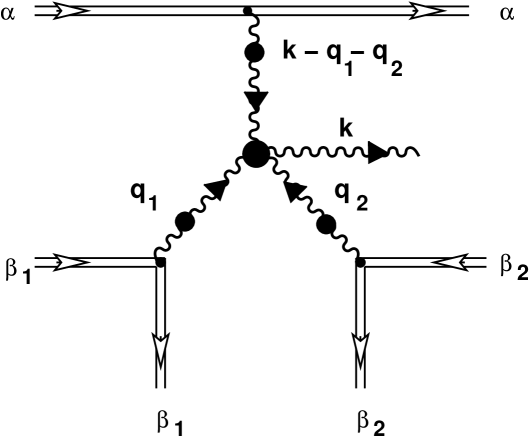
Figure 7: The transition bremsstrahlung induced by $\delta\Gamma_{4g}$ vertex HTL correction.

In the case of bare four-gluon vertex $\Gamma_{4g}$ this contribution is usually dropped for kinematic reason associated with absence of momentum dependence of $\Gamma_{4g}$ [3, 4]. The momentum dependence of $\delta\Gamma_{4g}$ on incoming lines is very nontrivial, and here we can expect an appreciable contribution of new mechanism of bremsstrahlung to gluon radiation intensity. If we restrict our consideration to this case, then under partial coefficient function in Eq. (9.3) we mean expression

$$K_{\mu}({\bf v}_{\alpha},{\bf v}_{\beta_{1}},{\bf v}_{\beta_{2}};{\bf x}_{10},{\bf x}_{20}|\,k)=\int\!{\cal K}_{\mu}({\bf v}_{\alpha},{\bf v}_{\beta_{1}},{\bf v}_{\beta_{2}}|\,k,q_{1},q_{2})\delta(v_{\alpha}\cdot(k-q_{1}-q_{2}))\delta(v_{{\beta}_{1}}\cdot q_{1})\delta(v_{{\beta}_{2}}\cdot q_{2})$$

$$\times\,{\rm e}^{i{\bf x}_{10}\cdot\,{\bf q}_{1}}{\rm e}^{i{\bf x}_{20}\cdot\,{\bf q}_{2}}dq_{10}dq_{20}d{\bf q}_{1}d{\bf q}_{2},$$ (9.4)

where

$${\cal K}_{\mu}({\bf v}_{\alpha},{\bf v}_{\beta_{1}},{\bf v}_{\beta_{2}}|\,k,q_{1},q_{2})\equiv\delta\Gamma_{\mu\nu\lambda\sigma}(k,-q_{1},-q_{2},-k+q_{1}+q_{2})\,^{\ast}{\cal D}_{C}^{\nu\nu^{\prime}}(q_{1})v_{\beta_{1}\nu^{\prime}}\!\,^{\ast}{\cal D}_{C}^{\lambda\lambda^{\prime}}(q_{2})v_{\beta_{2}\lambda^{\prime}}$$

$$\times\,^{\ast}{\cal D}_{C}^{\sigma\sigma^{\prime}}(k-q_{1}-q_{2})v_{\alpha\sigma^{\prime}}.$$ (9.5)

Now we substitute an effective current (9.3) into Eq. (9.1) and average over initial values of color charges, taking into account a relation for color algebra (7.6). Keeping in propagator $\!\,{}^{\ast}{\cal D}_{C}^{\mu\nu}(k)$ a transverse part only with allowance for (3.5) and going over to mass-shell of radiated transverse gluon (Eq. (3.10)), after simple algebraic transformations we lead to the expression for radiation field energy

$$W({\bf x}_{10},{\bf x}_{20})=\frac{1}{(2\pi)^{4}}\,\biggl{(}\frac{{\alpha}_{s}}{\pi}\biggr{)}^{\!5}\,C_{A}^{\,2}\Biggl{(}\frac{C_{2}^{(\alpha)}C_{2}^{(\beta_{1})}C_{2}^{(\beta_{2})}}{d_{A}^{2}}\Biggr{)}\!\sum_{\zeta=1,\,2}\!\int\!d{\bf k}\,\omega_{\bf k}^{t}\left(\frac{{\rm Z}_{t}({\bf k})}{2\omega_{\bf k}^{t}}\right)$$ (9.6)

$$\times\biggl{\{}|\,K^{i}({\bf v}_{\alpha},{\bf v}_{\beta_{1}},{\bf v}_{\beta_{2}};{\bf x}_{10},{\bf x}_{20}|\,k){\rm e}^{i}(\hat{\bf k},\zeta)|^{\,2}+|\,K^{i}({\bf v}_{\alpha},{\bf v}_{\beta_{2}},{\bf v}_{\beta_{1}};{\bf x}_{20},{\bf x}_{10}|\,k){\rm e}^{i}(\hat{\bf k},\zeta)|^{\,2}$$

$$+\,{\rm Re}\Bigl{[}\Bigl{(}\,K^{i}({\bf v}_{\alpha},{\bf v}_{\beta_{1}},{\bf v}_{\beta_{2}};{\bf x}_{10},{\bf x}_{20}|\,k){\rm e}^{i}(\hat{\bf k},\zeta)\Bigr{)}^{\!\ast}\Bigl{(}K^{j}({\bf v}_{\alpha},{\bf v}_{\beta_{2}},{\bf v}_{\beta_{1}};{\bf x}_{20},{\bf x}_{10}|\,k){\rm e}^{j}(\hat{\bf k},\zeta)\Bigr{)}\Bigr{]}\!\biggr{\}}.$$

Let us consider module squared $|K^{i}{\rm e}^{i}|^{2}$ in integrand. Substituting an expression (9.4) instead of $K^{i}$ and performing integration over $dq_{10}dq_{20}dq_{10}^{\prime}dq_{20}^{\prime}$, we obtain

$$|\,K^{i}({\bf v}_{\alpha},{\bf v}_{\beta_{1}},{\bf v}_{\beta_{2}};{\bf x}_{10},{\bf x}_{20}|\,k){\rm e}^{i}(\hat{\bf k},\zeta)|^{\,2}=\!\int\!\Bigl{[}\,{\cal K}^{i}({\bf v}_{\alpha},{\bf v}_{\beta_{1}},{\bf v}_{\beta_{2}}|\,k,q_{1},q_{2}){\rm e}^{i}(\hat{\bf k},\zeta)\Bigr{]}_{q^{0}_{1,2}={{\bf v}_{\beta_{1,2}}}\cdot\,{{\bf q}_{1,2}}}$$ (9.7)

$$\times\Bigl{[}\,{\cal K}^{j}({\bf v}_{\alpha},{\bf v}_{\beta_{1}},{\bf v}_{\beta_{2}}|\,k,q_{1}^{\prime},q_{2}^{\prime}){\rm e}^{j}(\hat{\bf k},\zeta)\Bigr{]}^{\ast}_{q^{\prime 0}_{1,2}={{\bf v}_{\beta_{1,2}}}\cdot\,{{\bf q}_{1,2}^{\prime}}}\delta(\omega_{\bf k}^{t}-{\bf v}_{\beta_{1}}\cdot{{\bf q}_{1}}-{\bf v}_{\beta_{2}}\cdot{{\bf q}_{2}}-{\bf v}_{\alpha}\cdot({\bf k}-{\bf q}_{1}-{\bf q}_{2}))$$

$$\times\,\delta(({\bf v}_{\alpha}-{\bf v}_{\beta_{1}})\!\cdot\!({\bf q}_{1}-{\bf q}_{1}^{\prime})+({\bf v}_{\alpha}-{\bf v}_{\beta_{2}})\!\cdot\!({\bf q}_{2}-{\bf q}_{2}^{\prime})){\rm e}^{i({\bf q}_{1}-{\bf q}_{1}^{\prime})\cdot{\bf x}_{10}}{\rm e}^{i({\bf q}_{2}-{\bf q}_{2}^{\prime})\cdot{\bf x}_{20}}d{\bf q}_{1}d{\bf q}_{2}d{\bf q}_{1}^{\prime}d{\bf q}_{2}^{\prime}.$$

Furthermore we analyze the expression in the last line of Eq. (9.7). We present vector ${\bf x}_{10}$ in the form of an expansion in terms of vectors system: the vector along relative velocity ${\bf v}_{\alpha}-{\bf v}_{\beta_{1}}$ and the vector orthogonal to ${\bf v}_{\alpha}-{\bf v}_{\beta_{1}}$, i.e. ${\bf x}_{10}=({\bf b}_{1}\equiv({\bf x}_{10})_{\perp},({\bf x}_{10})_{\|}).$ In this case a scalar product in the argument of the first exponential can be presented as

$$({\bf q}_{1}-{\bf q}_{1}^{\prime})\cdot{\bf x}_{10}=({\bf q}_{1}-{\bf q}_{1}^{\prime})_{\|}({\bf x}_{10})_{\|}+({\bf q}_{1}-{\bf q}_{1}^{\prime})_{\perp}\cdot{\bf b}_{1}.$$

The vector ${\bf b}_{1}$ is impact parameter of particle $\alpha$ relative to particle $\beta_{1}$. In a similar way we present vector ${\bf x}_{20}$ in the form of an expansion in terms of basis associated with vector of relative velocity ${\bf v}_{\alpha}-{\bf v}_{\beta_{2}}$: ${\bf x}_{20}=({\bf b}_{2}\equiv({\bf x}_{20})_{\perp},({\bf x}_{20})_{\|}).$ Then a scalar product in the argument of second exponential can be written in the form

$$({\bf q}_{2}-{\bf q}_{2}^{\prime})\cdot{\bf x}_{20}=({\bf q}_{2}-{\bf q}_{2}^{\prime})_{\|}({\bf x}_{20})_{\|}+({\bf q}_{2}-{\bf q}_{2}^{\prime})_{\perp}\cdot{\bf b}_{2}.$$

In this case vector ${\bf b}_{2}$ is impact parameter of particle $\alpha$ relative to particle $\beta_{2}$. By virtue of the fact that vectors ${\bf v}_{\alpha},\;{\bf v}_{{\beta}_{1}}$ and ${\bf v}_{{\beta}_{2}}$ are fixed, such representation of scalar products is uniquely determined.

With allowance for above-mentioned the following equality will be hold

$$\delta(({\bf v}_{\alpha}-{\bf v}_{\beta_{1}})\!\cdot\!({\bf q}_{1}-{\bf q}_{1}^{\prime})+({\bf v}_{\alpha}-{\bf v}_{\beta_{2}})\!\cdot\!({\bf q}_{2}-{\bf q}_{2}^{\prime})){\rm e}^{i({\bf q}_{1}-{\bf q}_{1}^{\prime})\cdot{\bf x}_{10}}{\rm e}^{i({\bf q}_{2}-{\bf q}_{2}^{\prime})\cdot{\bf x}_{20}}$$

$$=\delta(|\,{\bf v}_{\alpha}-{\bf v}_{\beta_{1}}\!|({\bf q}_{1}-{\bf q}_{1}^{\prime})_{\|}+|\,{\bf v}_{\alpha}-{\bf v}_{\beta_{2}}\!|({\bf q}_{2}-{\bf q}_{2}^{\prime})_{\|}){\rm e}^{i({\bf q}_{1}-{\bf q}_{1}^{\prime})_{\perp}\!\cdot{\bf b}_{1}}{\rm e}^{i({\bf q}_{2}-{\bf q}_{2}^{\prime})_{\perp}\!\cdot{\bf b}_{2}}$$ (9.8)

$$\times\frac{1}{2}\left\{\exp\left[i\,l\,\frac{{\cal V}}{|\,{\bf v}_{\alpha}-{\bf v}_{\beta_{1}}\!|}\,({\bf q}_{2}-{\bf q}_{2}^{\prime})_{\|}\right]+\exp\left[-i\,l\,\frac{{\cal V}}{|\,{\bf v}_{\alpha}-{\bf v}_{\beta_{2}}\!|}\,({\bf q}_{1}-{\bf q}_{1}^{\prime})_{\|}\right]\right\},$$

where in the last line we have

$${\cal V}\equiv 2\left(\frac{1}{|\,{\bf v}_{\alpha}-{\bf v}_{\beta_{1}}\!|}+\frac{1}{|\,{\bf v}_{\alpha}-{\bf v}_{\beta_{2}}\!|}\right)^{\!\!-1}\!,\quad l\equiv\frac{|\,{\bf v}_{\alpha}-{\bf v}_{\beta_{1}}\!|({\bf x}_{20})_{\|}-|\,{\bf v}_{\alpha}-{\bf v}_{\beta_{2}}\!|({\bf x}_{10})_{\|}}{\cal V}\,.$$

After integrating Eq. (9.8) over $d{\bf b}_{1}$, $d{\bf b}_{2}$ and $dl$, we derive

$$\frac{(2\pi)^{5}}{\cal V}\,\delta^{(2)}(({\bf q}_{1}-{\bf q}_{1}^{\prime})_{\perp})\delta(({\bf q}_{1}-{\bf q}_{1}^{\prime})_{\|})\delta^{(2)}(({\bf q}_{2}-{\bf q}_{2}^{\prime})_{\perp})\delta(({\bf q}_{2}-{\bf q}_{2}^{\prime})_{\|}),$$

that enables us to perform integration in Eq. (9.7) over $d{\bf q}_{1}^{\prime}d{\bf q}_{2}^{\prime}$. Now we write an expression for the gluon radiation intensity for the case of two nonrelativisic scatterers

$$\left\langle\frac{dW({\bf b}_{1},{\bf b}_{2},l)}{dt}\right\rangle_{\!{\bf b}_{1}\!,\,{\bf b}_{2}\!,\,l}=\int\!d{\bf b}_{1}d{\bf b}_{2}\!\int\!\!dl\!\int\!f_{{\bf p}_{{\beta}_{1}}}\,\frac{d{\bf p}_{{\beta}_{1}}}{(2\pi)^{3}}\,\int\!f_{{\bf p}_{{\beta}_{2}}}\,\frac{d{\bf p}_{{\beta}_{2}}}{(2\pi)^{3}}\,W({\bf b}_{1},{\bf b}_{2},l)\,{\cal V}.$$

Substituting (9.6) in this expression, taking into account (9.7) and (9.8), we obtain a final expression for gluon radiation intensity

$$\left\langle\frac{dW({\bf b}_{1},{\bf b}_{2},l)}{dt}\right\rangle_{\!{\bf b}_{1}\!,\,{\bf b}_{2}\!,\,l}=\frac{{\alpha}_{s}^{5}}{\pi^{4}}\,C_{A}^{2}\!\sum_{{\beta}_{1},{\beta}_{2}}\!\Biggl{(}\frac{C_{2}^{(\alpha)}C_{2}^{(\beta_{1})}C_{2}^{(\beta_{2})}}{d_{A}}\Biggr{)}\!\Biggl{(}\int\!{\bf p}_{\beta_{1}}^{2}f_{|{\bf p}_{\beta_{1}}|}\,\frac{d|{\bf p}_{\beta_{1}}|}{2\pi^{2}}\Biggr{)}\!\Biggl{(}\int\!{\bf p}_{\beta_{2}}^{2}f_{|{\bf p}_{\beta_{2}}|}\,\frac{d|{\bf p}_{\beta_{2}}|}{2\pi^{2}}\Biggr{)}$$

$$\times\int\!\frac{d\Omega_{{\bf v}_{\beta_{1}}}}{4\pi}\!\int\!\frac{d\Omega_{{\bf v}_{\beta_{2}}}}{4\pi}\!\sum_{\zeta=1,\,2}\!\int\!d{\bf k}\,\omega_{\bf k}^{t}\left(\frac{{\rm Z}_{t}({\bf k})}{2\omega_{\bf k}^{t}}\right)\!\!\int\!d{\bf q}_{1}d{\bf q}_{2}\,\delta(\omega_{\bf k}^{t}-{\bf v}_{\beta_{1}}\cdot{{\bf q}_{1}}-{\bf v}_{\beta_{2}}\cdot{{\bf q}_{2}}-{\bf v}_{\alpha}\cdot({\bf k}-{\bf q}_{1}-{\bf q}_{2}))$$

$$\times\biggl{\{}|\,{\cal K}^{i}({\bf v}_{\alpha},{\bf v}_{\beta_{1}},{\bf v}_{\beta_{2}}|\,k,q_{1},q_{2}){\rm e}^{i}(\hat{\bf k},\zeta)|^{\,2}+|\,{\cal K}^{i}({\bf v}_{\alpha},{\bf v}_{\beta_{2}},{\bf v}_{\beta_{1}}|\,k,q_{2},q_{1}){\rm e}^{i}(\hat{\bf k},\zeta)|^{\,2}$$ (9.9)

$$+{\rm Re}\Bigl{[}\Bigl{(}{\cal K}^{i}({\bf v}_{\alpha},{\bf v}_{\beta_{1}},{\bf v}_{\beta_{2}}|\,k,q_{1},q_{2}){\rm e}^{i}(\hat{\bf k},\zeta)\Bigr{)}^{\ast}\!\Bigl{(}{\cal K}^{i}({\bf v}_{\alpha},{\bf v}_{\beta_{2}},{\bf v}_{\beta_{1}}|\,k,q_{2},q_{1}){\rm e}^{i}(\hat{\bf k},\zeta)\Bigr{)}\Bigr{]}\!\biggr{\}}_{\omega=\omega_{\bf k}^{t}\!,\,q^{0}_{1,2}={{\bf v}_{\beta_{1,2}}}\cdot\,{{\bf q}_{1,2}}}.$$

Furthermore we restrict our consideration to limit of static color centers, i.e. we set ${\bf v}_{\beta_{1}}={\bf v}_{\beta_{2}}=0$. (In this case variable $l$ in Eq. (9.8) coincides with the longitudinal separation between two color static center $\beta_{1}$ and $\beta_{2}$.) Taking into account Eq. (4.2) and keeping in the effective propagator $\,{}^{\ast}{\cal D}_{C}^{\sigma\sigma^{\prime}}(k-q_{1}-q_{2})v_{\alpha\sigma^{\prime}}$ transverse part only, we derive for special case (9.5)

$${\cal K}^{i}({\bf v}_{\alpha},0,0|\,k,q_{1},q_{2}){\rm e}^{i}(\hat{\bf k},\zeta)|_{q_{1}^{0}=q_{2}^{0}=0}=\frac{1}{({\bf q}_{1}^{2}+\mu_{D}^{2})}\,\frac{1}{({\bf q}_{2}^{2}+\mu_{D}^{2})}\,^{\ast}{\!\Delta}^{t}(\omega,{\bf k}-{\bf q}_{1}-{\bf q}_{2})$$

$$\times\Bigl{[}\,{\rm e}^{i}(\hat{\bf k},\zeta)\delta\Gamma^{i00j}(k,-q_{1},-q_{2},-k+q_{1}+q_{2})v_{\alpha}^{j}\Bigr{]}_{q_{1}^{0}=q_{2}^{0}=0},$$

where four-gluon HTL vertex correction is defined by [74, 75]

$$\delta\Gamma^{i00j}(k,-q_{1},-q_{2}-k+q_{1}+q_{2})|_{\,q_{1}^{0}=q_{1}^{0}=0}$$ (9.10)

$$=-\mu_{D}^{2}\,{\omega}\!\int\!\frac{d{\Omega}_{\bf v}}{4\pi}\,\frac{v^{i}v^{j}}{v\cdot k}\,\,\frac{1}{v\cdot(k-q_{1})+i\epsilon}\,\frac{1}{v\cdot(k-q_{1}-q_{2})+i\epsilon}.$$

Now our problem is to show that function (9.10) contains singularity similar to that of vertex function (5.3) considered above, associated with zeros of function $\delta$, Eq. (5.6). The existence of such singularity enables us at least in principle in spirit of Section 5 to simplify analysis of expression for energy loss (9.9) and perform it to a great extent by analytic.

Let us define an explicit form of integral on the right-hand side of Eq. (9.10) replacing at the moment for convenience

$$k\rightarrow k_{1},\quad k-q_{1}\rightarrow k_{2},\quad k-q_{1}-q_{2}\rightarrow k_{3}.$$ (9.11)

In this case the analog of expansion (5.3) is

$$\int\!\frac{d{\Omega}_{\bf v}}{4\pi}\,\frac{v^{i}v^{j}}{(v\cdot k_{1})(v\cdot k_{2})(v\cdot k_{3})}=Y_{1}n_{1}^{i}n_{1}^{j}+Y_{2}n_{2}^{i}n_{2}^{j}+Y_{3}n_{3}^{i}n_{3}^{j}$$ (9.12)

$$+\,Z_{12}(n_{1}^{i}n_{2}^{j}+n_{1}^{j}n_{2}^{i})+Z_{13}(n_{1}^{i}n_{3}^{j}+n_{1}^{j}n_{3}^{i})+Z_{23}(n_{2}^{i}n_{3}^{j}+n_{2}^{j}n_{3}^{i}).$$

Here, ${\bf n}_{1}=[{\bf k}_{2},{\bf k}_{3}],\;{\bf n}_{2}=[{\bf k}_{3},{\bf k}_{1}]$ and ${\bf n}_{3}=[{\bf k}_{1},{\bf k}_{2}]$. Chosen basis is very convenient by virtue of properties

$${\bf k}_{s}\cdot{\bf n}_{l}=0,\;\,{\rm if}\;s\neq l;\quad{\bf k}_{1}\cdot{\bf n}_{1}={\bf k}_{2}\cdot{\bf n}_{2}={\bf k}_{3}\cdot{\bf n}_{3}.$$

The explicit form of coefficient functions $Y_{s},Z_{sl}$, $s\!<\!l,\,s,l=1,2,3$ is defined in Appendix B. They have following general structure

$$Y_{s}=\frac{1}{\delta^{\prime}}\,\tilde{Y}_{s},\quad Z_{sl}=\frac{1}{\delta^{\prime}}\,\tilde{Z}_{sl},$$ (9.13)

where functions $\tilde{Y}_{s}$ and $\tilde{Z}_{sl}$ are given by Eqs. (B.1) and (B.2), and determinant

$$\delta^{\prime}=\left|\begin{array}[]{lcr}{\bf k}^{2}_{1}&{\bf k}_{1}\cdot{\bf k}_{2}&{\bf k}_{1}\cdot{\bf k}_{3}\\ {\bf k}_{1}\cdot{\bf k}_{2}&{\bf k}_{2}^{2}&{\bf k}_{2}\cdot{\bf k}_{3}\\ {\bf k}_{1}\cdot{\bf k}_{3}&{\bf k}_{2}\cdot{\bf k}_{3}&{\bf k}^{2}_{3}\end{array}\right|$$ (9.14)

represents Gramian for three-dimensional vectors ${\bf k}_{1},\,{\bf k}_{2},$ and ${\bf k}_{3}$. As known vanishing of this determinant gives necessary and sufficient condition of complanarity of these vectors. Note that condition (5.6) also can be written in the form of Gramian, and such in this case condition $\delta=0$ will yields condition of collinearity of vectors ${\bf k}$ and ${\bf q}^{\prime}$.

We return now to variables (9.11) and consider equation

$$\delta^{\prime}\equiv\left|\begin{array}[]{lcr}{\bf k}^{2}&{\bf k}\cdot{\bf q}_{1}^{\prime}&{\bf k}\cdot{\bf q}_{2}^{\prime}\\ {\bf k}_{1}\cdot{\bf q}_{1}^{\prime}&{\bf q}_{1}^{\prime 2}&{\bf q}_{1}^{\prime}\cdot{\bf q}_{2}^{\prime}\\ {\bf k}_{1}\cdot{\bf q}_{2}^{\prime}&{\bf q}_{1}^{\prime}\cdot{\bf q}_{2}^{\prime}&{\bf q}_{2}^{\prime 2}\end{array}\right|=0\,,$$ (9.15)

where ${\bf q}_{1}^{\prime}\equiv{\bf k}-{\bf q}_{1}$, ${\bf q}_{\,2}^{\prime}\equiv{\bf k}-{\bf q}_{1}-{\bf q}_{2}$. Delta-function in the integrand (9.9) enables us to fix only $q_{2\|}^{\prime}=\omega_{\bf k}^{t}/v_{\alpha}$. We choose coordinate system as depicted in Fig. 2, axis $0Z$ is aligned with the velocity ${\bf v}_{\alpha}$. In chosen coordinate system we have ${\bf k}=(|{\bf k}|,\theta,\varphi),\;{\bf q}_{1}^{\prime}=(|{\bf q}_{1}^{\prime}|,\vartheta,\beta_{1}),\;{\bf q}_{\,2\perp}^{\prime}=(|{\bf q}_{2\perp}^{\prime}|,\pi/2,\beta_{2})$, and correspondingly integration measures are

$$d{\bf k}={\bf k}^{2}d|{\bf k}|\sin\theta d\theta d\varphi,\quad d{\bf q}_{1}^{\prime}={\bf q}_{1}^{\prime\,2}d|{\bf q}_{1}^{\prime}|\sin\vartheta d\vartheta d\beta_{2},\quad d{\bf q}_{2\perp}^{\prime}=|{\bf q}_{2\perp}^{\prime}|d|{\bf q}_{2\perp}^{\prime}|d\beta_{2}.$$

On the conditions ${\bf k}^{2}\neq 0$, ${\bf q}_{1}^{\prime\,2}\neq 0$ equation (9.15) can be presented as

$$(1+\chi^{2})\Bigl{[}1-(\sin\theta\sin\vartheta\cos(\varphi-\beta_{1})+\cos\theta\cos\vartheta)^{2}\,\bigr{]}$$ (9.16)

$$+\,\Bigl{[}\,(1+\chi^{2})-(\chi\sin\theta\cos(\varphi-\beta_{2})+\cos\theta)^{2}\,\Bigr{]}+\,\Bigl{[}\,(1+\chi^{2})-(\chi\sin\vartheta\cos(\beta_{1}-\beta_{2})+\cos\vartheta)^{2}\,\Bigr{]}=0.$$

Here, $\chi\equiv v_{\alpha}|{\bf q}_{2\perp}^{\prime}|/\omega$. This equation represents appropriate extension of Eq. (5.7). Note that angle $\beta_{2}$ will be enter everywhere as difference with azimuth angles $\varphi$ and $\beta_{1}$, and therefore it can be set equal to zero and integral is $\int d\beta_{2}=2\pi$.

We can obtain simplest nontrivial solution of this equation if we set expressions in two last square brackets on the left-hand side of Eq. (9.16) equal to zero. The solution have a form

$$\cos\varphi_{\pm}=-\,\frac{1}{\chi\sin\theta}\,\Bigl{(}\cos\theta\mp\sqrt{1+{\chi}^{2}}\,\Bigr{)},\quad\cos\beta_{1\pm}=-\,\frac{1}{\chi\sin\vartheta}\,\Bigl{(}\cos\vartheta\mp\sqrt{1+{\chi}^{2}}\,\Bigr{)}.$$ (9.17)

It is not difficult to see that in deciding of (9.17) the expression in first square brackets vanishes. This solution is correspondent to the case already considered in Section 5, and therefore performed analysis of transition bremsstrahlung can be extended to this problem. However solution (9.17) represents very hard condition for vanishing of function $\delta^{\prime}$. It corresponds to condition of collinearity of three vectors ${\bf k},\;{\bf q}_{1}^{\prime}$ and ${\bf q}_{2}^{\prime}$. In general case it is necessary to solve algebraic equation (9.16), that in notation $x\equiv\cos\varphi,\;y\equiv\cos\beta_{1}$, can be written in more clear form

$$\Bigl{[}\,a\Bigl{(}xy-\sqrt{(1-x^{2})(1-y^{2})}\,\Bigr{)}+b\,\Bigr{]}^{\,2}+(c_{\theta}x+d_{\theta})^{2}+(c_{\vartheta}y+d_{\vartheta})^{2}-3=0,$$

where

$$a=\sin\theta\sin\vartheta,\;b=\cos\theta\cos\vartheta,\;c_{\theta}=\tanh\xi\sin\theta,\;c_{\vartheta}=\tanh\xi\sin\vartheta,$$

$$d_{\theta}=\frac{\cos\theta}{\cosh\xi},\;\quad d_{\vartheta}=\frac{\cos\vartheta}{\cosh\xi},\quad\xi\equiv\ln\Bigl{(}\chi+\sqrt{1+\chi^{2}}\,\Bigr{)},\quad\chi=\sinh\xi.$$

At the end of this Section we briefly analyze a case of transition bremsstrahlung in scattering of energetic parton $\alpha$ off three static color centers, the process proceeding through five soft gluon HTL induced vertex, as depicted on Fig. 8. In the case of radiation of transverse

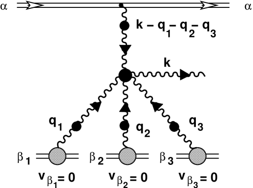
Figure 8: Transition bremsstrahlung induced by $\delta\Gamma_{5g}$ vertex HTL correction.

soft gluon, calculation of matrix element of this process is reduced to calculation of integral in the form

$$\int\!\frac{d{\Omega}_{\bf v}}{4\pi}\,\frac{v^{i}v^{j}}{(v\cdot k_{1})(v\cdot k_{2})(v\cdot k_{3})(v\cdot k_{4})},$$

where $k_{1}=k,\;k_{2}=k-q_{1},\;k_{3}=k-q_{1}-q_{2}$ and $k_{4}=k-q_{1}-q_{2}-q_{3}$. According reasoning of Frenkel and Taylor [74], this integral represents pure spatial part of Lorentz-covariant tensor of 2-rank

$$U^{\mu\nu}=\int\!\frac{d{\Omega}_{\bf v}}{4\pi}\,\frac{v^{\mu}v^{\nu}}{(v\cdot k_{1})(v\cdot k_{2})(v\cdot k_{3})(v\cdot k_{4})}.$$

This integral can be presented in the form of expansion in basis

$$U^{\mu\nu}=\sum\limits_{s=1}^{4}\!A_{s}n_{s}^{\mu}n_{s}^{\nu}+\sum\limits_{s<l}\!B_{s\,l}\,(n_{s}^{\mu}n_{l}^{\nu}+n_{l}^{\mu}n_{s}^{\nu}),\quad s,\,l=1,2,3,4\,,$$ (9.18)

where we enter 4-vectors

$$n_{1}^{\mu}=\varepsilon^{\mu\nu\lambda\sigma}k_{2}^{\nu}k_{3}^{\lambda}k_{4}^{\sigma},\quad n_{2}^{\mu}=\varepsilon^{\mu\nu\lambda\sigma}k_{3}^{\nu}k_{4}^{\lambda}k_{1}^{\sigma},\quad n_{3}^{\mu}=\varepsilon^{\mu\nu\lambda\sigma}k_{4}^{\nu}k_{1}^{\lambda}k_{2}^{\sigma},\quad n_{4}^{\mu}=\varepsilon^{\mu\nu\lambda\sigma}k_{1}^{\nu}k_{2}^{\lambda}k_{3}^{\sigma},$$

and $\varepsilon^{\mu\nu\lambda\sigma}$ is absolute antisymmetric tensor of 4-rank. In Appendix C calculation of coefficients $A_{s}$ and $B_{s\,l},\;s<l$ are given. They have following general structure analogous to (9.13)

$$A_{s}=\frac{1}{\Delta^{\prime\prime}}\,\tilde{A}_{s},\quad Z_{sl}=\frac{1}{\Delta^{\prime\prime}}\,\tilde{B}_{s\,l},$$ (9.19)

where the functions $\tilde{A}_{s}$ and $\tilde{B}_{sl}$ are given by expressions (C.1) and (C.2), correspondingly, and

$$\Delta^{\prime\prime}=(\varepsilon^{\mu\nu\lambda\sigma}k_{1\mu}k_{2\nu}k_{3\lambda}k_{4\sigma})^{2}=-\left|\begin{array}[]{lccr}k_{1}^{2}&k_{1}\cdot k_{2}&k_{1}\cdot k_{3}&k_{1}\cdot k_{4}\\ k_{1}\cdot k_{2}&k_{2}^{2}&k_{2}\cdot k_{3}&k_{2}\cdot k_{4}\\ k_{1}\cdot k_{3}&k_{2}\cdot k_{3}&k_{3}^{2}&k_{3}\cdot k_{4}\\ k_{1}\cdot k_{4}&k_{2}\cdot k_{4}&k_{3}\cdot k_{4}&k_{4}^{2}\end{array}\right|$$ (9.20)

represents Gramian for 4-vectors $k_{1},\,k_{2},\,k_{3}$ and $k_{4}$. Zeros of determinant (9.20) define singular surface in a space of kinematic variables, on which it should be defined all functions in matrix element of this transition bremsstrahlung.

If we consider medium induced bremsstrahlung of higher-order than in Fig. 8, i.e. one in scattering off four, five etc. static color centers, then we can expect an absence of general singular factor as it occurs in coefficient functions (5.4), (9.13) and (9.19) by virtue of the fact that it is impossible to define nontrivial Gramian for five and more 4-vectors. Therefore we can suppose that these higher processes of transition bremsstrahlung will be strongly suppressed in comparison with lower-order processes (i.e. containing gluon vertices with smaller number of soft external legs) and thus they are not of our interest.

10 Summary and outlook

In this work in the framework of semiclassical approximation we have proposed an approach to calculation of radiation intensity of high-energy parton travelling through hot QCD medium. The deriving of some effective color currents generating bremsstrahlung processes of arbitrary number of soft gluons for scattering energetic parton off arbitrary number of thermal particles of medium is a great moment for this consideration.

A suggested scheme for calculation of these effective currents tacitly implies by virtue of initial dynamical equations that hot QCD medium represents a weakly coupled system $(g\ll 1)$, allowing to use perturbative approach. However theoretical analysis of experimental data, especially concerning with collective flow, unambiguously shows that properties of ‘new matter’ produced at RHIC experiments for moderate temperatures $(1\div 3)T_{c}$ substantially different from the expectation of a weakly coupled colored plasma (see the last reviews on this subject [82, 83, 84, 85]). A major revision of proposed scheme to calculation of radiative energy loss can be one of the consequences of such conclusion. For example within standard Gyulassy-Wang model multiple scattering in medium is considered as totality of subsequent acts of pair interaction of particles, and in particular an influence of simultaneous collision of several (more then two) particles on formation of bremsstrahlung spectrum is neglected. It is clear that effects of such type can play an important role in the processes of gluon multiplication in rather dense scattering medium (e.g., liquid type), when plasma parameter $\Gamma$ becomes more or of the order of one. The attempt of taking into account of such effects in dense matter was made in work [86] for the case of bremsstrahlung of fast electric charged particles. Here, diagrammatic formalism for two-particle Green functions was used. It was shown that in the case of radiation in sufficiently dense medium in a distant long wavelength region of spectrum coherent multiple scattering of particles results in (supplementary to LPM effect) suppression of the yield of bremsstrahlung photons. We can expect that similar phenomenon has to take place and for the case of dense strongly coupled quark-gluon plasma ($s$QGP) for description of that a number of approaches is already proposed [88, 89, 90, 91].

The approach to calculation of effective currents suggested in this work (and in Papers I and II also) can be extended to the case of strongly coupled QGP. The use of collisionless Blaizot-Iancu equation (I.3.3) correctly describing behavior of QGP in the weakly coupling regime and at soft momentum scale of plasma density fluctuations is one of the most key moments for the derivation of effective color currents. Therefore as a first step of construction of the radiation energy loss theory in $s$QGP this kinetic equation is necessary to be extended in a way. As one of the leading ideas representations developed in attempt to describe thermodynamical properties, the transport coefficients and the dynamical correlations of strongly coupled usual plasma, can be used.

The extensive research of properties of usual plasma, when plasma parameter $\Gamma$ changes within huge region: from slowly coupling regime $\Gamma\ll 1$ and up to $\Gamma\sim 1000$ were undertaken more than 20 years ago. In particular, for a strongly coupled one-component plasma Vieillefosse and Hansen [92] and Wallenborn and Baus [93] have advanced theoretical estimations of the shear $\eta$ and the bulk viscosities on the basis of hydrodynamic and kinetic-theoretical arguments, correspondingly. The two calculations are in agreement shown that the transverse viscosity $\eta$ (exactly its dimensionless combination) exhibits a minimum as a function of $\Gamma$ (for values $\Gamma\sim 10\div 20$) and $\zeta$ is negligible compared to $\eta$. The value $\eta$ in a point of minimality is more little then a value for the weakly coupled plasma, when $\Gamma\ll 1$. This very important and striking observation was confirmed through molecular-dynamics computer simulations [94]. The position of the minimum is, however, rather sensitive to the various approximations.

Furthermore Tanaka and Ichimaru [95, 96] have developed a new kinetic theory of dynamic correlations for a strongly coupled, classical one-component plasma within the generalized viscoelastic formalism [97]. The strong Coulomb-coupling effects beyond random phase approximation are described in the present theory through the dynamic local-field correction $G({\bf k},\omega)$ introduced via linear-response relation between the external potential $\varphi_{\rm ext}({\bf k},\omega)$ and the induced density fluctuation $\delta n({\bf k},\omega)$. Making use a fully convergent kinetic equation originally proposed by them, where higher-order scattering processes are included through the factor $1-G({\bf k},\omega)$ in integrand of collision term, Tanaka, and Ichimaru have established a self-consistent scheme to calculate $\eta$ and $G({\bf k},\omega)$ simultaneously. Their predictions showed a good agreement with early obtained results of different approaches [92, 93, 94].

Performed researches for strongly coupled usual plasma suggest that in a case of classical $s$QGP we can also expect an existence of minimal value of the shear viscosity for some finite value of QCD plasma parameter (10.1) and this value can be appreciably smaller than value following from perturbative estimations [98, 99] for weakly coupled QGP. It is represented extremely important by virtue of very small value of $\eta$ for a new QCD matter discovered at RHIC experiments [100]. The requirement of minimality of shear viscosity has to lead to definite fixing of generalized collision term for kinetic equation, that in weakly coupled limit must turn to kinetic equation (I.3.3). Having in hand such an equation we can further develop an extended scheme for calculations of color effective currents generating bremsstrahlung processes (and radiative energy losses produced by them) of high-energy partons in the $s$QGP. The exact consideration of this approach will be the subject of a further research.

Appendix A

Here, we give complete expression for partial coefficient function $K_{\mu\mu_{1}}({\bf v}_{\alpha},{\bf v}_{\beta};{\bf b}|\,k,k_{1})$ defining bremsstrahlung of two soft gluons in scattering of energetic color particle $\alpha$ off hard thermal parton $\beta$

$$K_{\mu\mu_{1}}({\bf v}_{\alpha},{\bf v}_{\beta};{\bf b}|\,k,k_{1})=\int\!\biggl{\{}\frac{v_{\alpha\mu}v_{\alpha\nu}}{v_{\beta}\cdot(q-k_{1})}\,^{\ast}{\cal D}_{C}^{\nu\nu^{\prime}}\!(q-k_{1})K_{\nu^{\prime}\mu_{1}}({\bf v}_{\beta}|\,q-k_{1},k_{2})$$

$$+\,\frac{v_{\alpha\mu}v_{\alpha\mu_{1}}}{(v_{\alpha}\cdot(q-k_{1}))(v_{\alpha}\cdot q)}\,(v_{\alpha\nu}\!\,^{\ast}{\cal D}_{C}^{\nu\nu^{\prime}}\!(q)v_{\beta\nu^{\prime}})$$

$$+\,\frac{v_{\beta\mu}v_{\beta\mu_{1}}}{(v_{\beta}\cdot k_{1}))(v_{\beta}\cdot(k+k_{1}-q))}\,(v_{\beta\nu}\!\,^{\ast}{\cal D}_{C}^{\nu\nu^{\prime}}\!(k+k_{1}-q)v_{\alpha\nu^{\prime}})$$

$$+\,^{\ast}\Gamma_{\mu\nu\lambda}(k,k_{1}-q,-k-k_{1}+q)\,^{\ast}{\cal D}_{C}^{\nu\nu^{\prime}}\!(q-k_{1})K_{\nu^{\prime}\mu_{1}}({\bf v}_{\beta}|\,q-k_{1},k_{1})\,^{\ast}{\cal D}_{C}^{\lambda\lambda^{\prime}}\!(k+k_{1}-q)v_{\alpha\lambda}$$

$$+\,^{\ast}\Gamma_{\mu\mu_{1}\lambda}(k,k_{1},-k-k_{1})\,^{\ast}{\cal D}_{C}^{\lambda\lambda^{\prime}}\!(k+k_{1}){\cal K}_{\lambda^{\prime}}({\bf v}_{\alpha},{\bf v}_{\beta}|\,k+k_{1},q)$$

$$-\,^{\ast}\Gamma_{\mu\nu\lambda\mu_{1}}(k,-k-k_{1}+q,-q,k_{1})\,^{\ast}{\cal D}_{C}^{\nu\nu^{\prime}}\!(k+k_{1}-q)v_{\beta\nu^{\prime}}\,^{\ast}{\cal D}_{C}^{\lambda\lambda^{\prime}}\!(q)v_{\beta\lambda^{\prime}}\biggr{\}}$$

$$\times\,{\rm e}^{-i{\bf b}\cdot\,{\bf q}}\,\delta(v_{\alpha}\cdot(k+k_{1}-q))\delta(v_{\beta}\cdot q)dq.$$

Here, the functions $K_{\mu\mu_{1}}({\bf v}|\,k,k_{1})$ and ${\cal K}_{\mu}({\bf v}_{\alpha},{\bf v}_{\beta}|\,k,q)$ are defined by Eq. (2.10) and Eq. (3.7), correspondingly. The graphic interpretation of various terms in this expression is presented on Fig. 9. Remind that graphs, where radiation

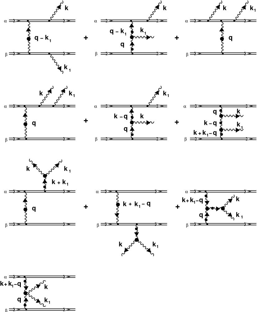
Figure 9: Two soft gluon bremsstrahlung.

lines from hard lines are located a prior one-gluon exchange, are not given here.

Below we adduce a complete expression for matrix element ${\cal K}^{(A)ii_{1}}{\rm e}^{i}{\rm e}^{i_{1}}$ in the high-frequency and small-angle approximations. This matrix element defines bremsstrahlung of two gluons forming odd state system (in the c.m.s. of gluons) with respect to space inversion

$${\cal K}^{(A)ii_{1}}({\bf v}_{\alpha},0|\,k,k_{1},q){\rm e}^{i}(\hat{\bf k},\zeta){\rm e}^{i_{1}}(\hat{\bf k}_{1},\zeta_{1})|_{\,q_{0}=0}$$

$$\simeq\frac{2}{{\bf q}_{\perp}+\mu_{D}^{2}+\displaystyle\frac{1}{v_{\alpha}^{2}}\left(\frac{1}{\tau_{f}}+\frac{1}{\tau_{\!1f}}\right)^{\!2}}\,\Biggl{[}\,\Biggl{(}\frac{\tau_{f}-\tau_{1f}}{\tau_{f}+\tau_{1f}}\Biggr{)}\frac{{\bf e}_{\perp}\cdot{\bf k}_{\perp}}{{\bf k}_{\perp}^{2}+m_{g}^{2}+x^{2}M^{2}}\,\,\frac{{\bf e}_{1\perp}\cdot{\bf k}_{1\perp}}{{\bf k}_{1\perp}^{2}+m_{g}^{2}+x_{1}^{2}M^{2}}$$

$$+\,\Biggl{\{}\,^{\ast}\!\Delta^{t}(q-k)\,\frac{({\bf e}_{\perp}\cdot({\bf k}-{\bf q})_{\perp})({\bf e}_{1\perp}\cdot{\bf k}_{1\perp})}{{\bf k}_{1\perp}^{2}+m_{g}^{2}+x_{1}^{2}M^{2}}\,-\,^{\ast}\!\Delta^{t}(q-k_{1})\,\frac{({\bf e}_{1\perp}\cdot({\bf k}_{1}-{\bf q})_{\perp})({\bf e}_{\perp}\cdot{\bf k}_{\perp})}{{\bf k}_{\perp}^{2}+m_{g}^{2}+x^{2}M^{2}}\Biggr{\}}$$

$$+\bigg{\{}\!\!\,^{\ast}\!\Delta^{t}(q-k_{1})\biggl{[}\Bigl{(}{\bf e}_{\perp}\cdot\Bigl{(}{\bf k}_{1}-\frac{x_{1}}{x}{\bf k}-{\bf q}\Bigr{)}_{\!\perp}\Bigr{)}({\bf e}_{1\perp}\cdot({\bf k}_{1}-{\bf q})_{\perp})+\Bigl{(}{\bf e}_{1\perp}\cdot\Bigl{(}{\bf k}_{1}-\frac{x_{1}}{x}{\bf k}-{\bf q}\Bigr{)}_{\!\perp}\Bigr{)}({\bf e}_{\perp}\cdot{\bf k}_{\perp})$$

$$+\,x_{1}\,\frac{({\bf e}_{\perp}\cdot{\bf e}_{1\perp})}{(x+x_{1})^{2}}\,\Bigl{[}\,x_{1}{\bf k}_{\perp}^{2}-x({\bf k}_{1}-{\bf q})^{2}_{\perp}-(x-x_{1})({\bf k}_{\perp}\cdot({\bf k}_{1}-{\bf q})_{\perp})\Bigr{]}\biggr{]}$$

$$+\,({\bf k}_{\perp}\rightleftharpoons{\bf k}_{1\perp},\,{\bf e}_{\perp}\rightleftharpoons{\bf e}_{1\perp},\,x\rightleftharpoons x_{1})\biggr{\}}\,^{\ast}\!\Delta^{t}(k+k_{1}-q)$$

$$+\,\,^{\ast}\!\Delta^{t}(k+k_{1})\Biggl{(}\frac{\omega+\omega_{1}}{\tau_{f}}+\frac{\omega+\omega_{1}}{\tau_{\!1f}}\Biggr{)}^{\!\!-1}\Biggr{\{}\Biggl{(}1+\frac{x}{x_{1}}\Biggr{)}\Bigl{(}{\bf e}_{\perp}\cdot\Bigl{(}{\bf k}_{1}-\frac{x_{1}}{x}{\bf k}\Bigr{)}_{\!\perp}\Bigr{)}({\bf e}_{1\perp}\cdot{\bf k}_{1\perp})$$

$$-\,\Biggl{(}1+\frac{x_{1}}{x}\Biggr{)}\Bigl{(}{\bf e}_{1\perp}\cdot\Bigl{(}{\bf k}-\frac{x}{x_{1}}{\bf k}_{1}\Bigr{)}_{\!\perp}\Bigr{)}({\bf e}_{\perp}\cdot{\bf k}_{\perp})+\frac{({\bf e}_{\perp}\cdot{\bf e}_{1\perp})}{x+x_{1}}\Bigl{[}\,x_{1}{\bf k}_{\perp}^{2}-x{\bf k}_{1\perp}^{2}-(x-x_{1})({\bf k}_{\perp}\cdot{\bf k}_{1\perp})\Bigr{]}\!\Biggr{\}}$$

$$+\,2\,^{\ast}\!\Delta^{t}(k+k_{1})\,^{\ast}\!\Delta^{t}(k+k_{1}-q)\biggr{\{}\Bigl{(}{\bf e}_{\perp}\cdot\Bigl{(}{\bf k}_{1}-\frac{x_{1}}{x}\,{\bf k}\Bigr{)}_{\!\perp}\Bigr{)}\Bigl{(}{\bf e}_{1\perp}\cdot\Bigl{(}\Bigl{(}1+\frac{x}{x_{1}}\Bigr{)}{\bf k}_{1}-{\bf q}\Bigr{)}_{\!\perp}\Bigr{)}$$

$$-\,\Bigl{(}{\bf e}_{1\perp}\cdot\Bigl{(}{\bf k}-\frac{x}{x_{1}}\,{\bf k}_{1}\Bigr{)}_{\!\perp}\Bigr{)}\Bigl{(}{\bf e}_{\perp}\cdot\Bigl{(}\Bigl{(}1+\frac{x_{1}}{x}\Bigr{)}{\bf k}-{\bf q}\Bigr{)}_{\!\perp}\Bigr{)}$$

$$+\,\frac{({\bf e}_{\perp}\cdot{\bf e}_{1\perp})}{x+x_{1}}\,\Bigl{[}\,x_{1}{\bf k}_{\perp}^{2}-x{\bf k}_{1\perp}^{2}-(x-x_{1})({\bf k}_{\perp}\cdot{\bf k}_{1\perp})-((x_{1}{\bf k}-x{\bf k}_{1})_{\perp}\cdot{\bf q}_{\perp})\Bigr{]}\biggr{\}}\Biggr{]},$$

where

$${}^{\ast}\!\Delta^{t}(k+k_{1})\simeq-\frac{1}{({\bf k}+{\bf k}_{1})^{2}_{\perp}+m_{g}^{2}-\displaystyle\Biggl{[}\Biggl{(}1+\frac{x_{1}}{x}\Biggr{)}({\bf k}_{\perp}^{2}+m_{g}^{2})+\Biggl{(}1+\frac{x}{x_{1}}\Biggr{)}({\bf k}_{1\perp}^{2}+m_{g}^{2})\Biggr{]}}\,.$$

The functions $\tau_{f}$, $\tau_{1f}$ are defined by Eq. (8.8) and the propagators $\,{}^{\ast}\!\Delta^{t}(q-k)$, $\,{}^{\ast}\!\Delta^{t}(q-k_{1})$ and ${}^{\ast}\!\Delta^{t}(k+k_{1}-q)$ are defined by Eqs. (8.8) and (8.11), correspondingly.

Appendix B

The coefficients $Y_{s},\;s=1,2,3$ in the expansion of (9.12) are defined by contracting with $k_{s}^{i}k_{s}^{j}$. Such, for example a contracting with $k_{1}^{i}k_{1}^{j}$ with use of identity

$$({\bf v}\cdot{\bf k}_{1})^{2}=\omega_{1}^{2}-2\omega_{1}(v\cdot k_{1})+(v\cdot k_{1})(\omega_{1}-{\bf v}\cdot{\bf k}_{1})$$

and formulas (3.24), (3.30) and (4.15) from [74] yields,

$$\delta^{\prime}\,Y_{1}=\tilde{Y}_{1}\equiv\omega_{1}^{2}[\,a\omega_{1}+b\,\omega_{2}+c\,\omega_{3}]-\omega_{1}M(k_{2},k_{3})$$

$$+\,\frac{1}{{\bf n}_{1}^{2}}\,\Bigl{\{}\Bigl{(}\omega_{2}({\bf n}_{1}\cdot{\bf n}_{2})+\omega_{3}({\bf n}_{1}\cdot{\bf n}_{3})\Bigr{)}M(k_{2},k_{3})-({\bf n}_{1}\cdot{\bf n}_{2})L(k_{3})-({\bf n}_{1}\cdot{\bf n}_{3})L(k_{2})\Bigr{\}},$$

where $\delta^{\prime}$ is defined by Eq. (9.14) and

$$a\equiv a(k_{1},k_{2},k_{3})=\frac{\Delta_{1}}{\Delta^{\prime}},\quad b\equiv b(k_{1},k_{2},k_{3})=\frac{\Delta_{2}}{\Delta^{\prime}},\quad c\equiv c(k_{1},k_{2},k_{3})=\frac{\Delta_{3}}{\Delta^{\prime}},$$

$$\Delta_{1}=\left|\begin{array}[]{lcr}M(k_{2},k_{3})&k_{1}\cdot k_{2}&k_{1}\cdot k_{3}\\ M(k_{1},k_{3})&k_{2}^{2}&k_{2}\cdot k_{3}\\ M(k_{1},k_{2})&k_{2}\cdot k_{3}&k_{3}^{2}\end{array}\right|\,,\quad\Delta_{2}=\left|\begin{array}[]{lcr}k_{1}^{2}&M(k_{2},k_{3})&k_{1}\cdot k_{3}\\ k_{1}\cdot k_{2}&M(k_{1},k_{3})&k_{2}\cdot k_{3}\\ k_{1}\cdot k_{3}&M(k_{1},k_{2})&k_{3}^{2}\end{array}\right|\,,$$

$$\Delta_{3}=\left|\begin{array}[]{lcr}k_{1}^{2}&k_{1}\cdot k_{2}&M(k_{2},k_{3})\\ k_{1}\cdot k_{2}&k_{2}^{2}&M(k_{1},k_{3})\\ k_{1}\cdot k_{3}&k_{2}\cdot k_{3}&M(k_{1},k_{2})\end{array}\right|\,,\quad\Delta^{\prime}=\left|\begin{array}[]{lcr}k_{1}^{2}&k_{1}\cdot k_{2}&k_{1}\cdot k_{3}\\ k_{1}\cdot k_{2}&k_{2}^{2}&k_{2}\cdot k_{3}\\ k_{1}\cdot k_{3}&k_{2}\cdot k_{3}&k_{3}^{2}\end{array}\right|\,,\hskip 25.6073pt$$

and functions $M(k,k_{1}),\,L(k)$ are defined by Eq. (5.5). The coefficients $Y_{2}$ and $Y_{3}$ are obtained in a similar way. They can be obtained from (B.1) by cyclic permutation of 1,2,3.

The coefficients $Z_{sl},\,s<l$ are defined by contracting (9.12) with $k_{s}^{i}k_{l}^{j}$. For example, a contracting with $k_{1}^{i}k_{2}^{j}$ yields an expression for $Z_{12}$

$$\delta^{\prime}Z_{12}=\tilde{Z}_{12}\equiv\omega_{1}\omega_{2}[\,a\omega_{1}+b\,\omega_{2}+c\,\omega_{3}]-\omega_{1}M(k_{1},k_{3})-\omega_{2}M(k_{2},k_{3})+L(k_{3}).$$

The remaining coefficients $Z_{13}$ and $Z_{23}$ follow from (B.3) by cyclic permutation of 1, 2, 3.

Now we add a term $X\delta^{ij}$ to the right-hand side of (9.12). In this case instead of relations (B.1) and (B.3) we will have

$$\delta^{\prime}Y_{s}+{\bf k}_{s}^{2}X=\tilde{Y}_{s},\quad\delta^{\prime}Z_{ls}+({\bf k}_{s}\cdot{\bf k}_{l})X=\tilde{Z}_{ls},\quad s<l;\;s,l=1,2,3.$$

The equation for $X$ is derived by taking of trace (9.12)

$$\tilde{X}\equiv\int\!\frac{d{\Omega}_{\bf v}}{4\pi}\,\frac{1}{(v\cdot k_{1})(v\cdot k_{2})(v\cdot k_{3})}=\,a\omega_{1}+b\,\omega_{2}+c\,\omega_{3}$$

$$=3X+\sum\limits_{s=1}^{3}{\bf n}_{s}^{2}Y_{s}+2\sum\limits_{s<l}({\bf n}_{s}\cdot{\bf n}_{l})Z_{sl}.$$

If we substitute (B.4) into the rightmost expression in (B.5) and collect similar terms, then we will have an equation for $X$

$$\tilde{X}=\frac{1}{\delta^{\prime}}\,X\biggl{[}\,3\delta^{\,\prime}-\Bigl{(}\sum\limits_{s=1}^{3}{\bf k}_{s}^{2}{\bf n}_{s}^{2}+2\sum\limits_{s<l}({\bf k}_{s}\cdot{\bf k}_{l})({\bf n}_{s}\cdot{\bf n}_{l})\Bigl{)}\biggr{]}+\frac{1}{\delta^{\prime}}\biggl{[}\,\sum\limits_{s=1}^{3}{\bf n}_{s}^{2}\tilde{Y}_{s}+2\sum\limits_{s<l}({\bf n}_{s}\cdot{\bf n}_{l})\tilde{Z}_{sl}\biggr{]}.$$

Let us consider an expression in square brackets in the first term on the right-hand side of Eq. (B.6). By virtue of the fact that scalar production represents algebraical adjunct to element $(ij)$ in Gramian (9.14), then

$${\bf k}_{s}^{2}{\bf n}_{s}^{2}+2\sum\limits_{l\neq s}({\bf k}_{s}\cdot{\bf k}_{l})({\bf n}_{s}\cdot{\bf n}_{l})=\delta^{\prime}\quad(\mbox{no summation over $s$!})$$

for all $s=1,2,3$. Therefore a factor after $X$ exactly vanishes. Let us show that the following identity is true

$$\tilde{X}=\frac{1}{\delta^{\prime}}\biggl{[}\,\sum\limits_{s=1}^{3}{\bf n}_{s}^{2}\tilde{Y}_{s}+2\sum\limits_{s<l}({\bf n}_{s}\cdot{\bf n}_{l})\tilde{Z}_{sl}\biggr{]}.$$

If one substitute instead of $\tilde{Y}_{s}$ and $\tilde{Z}_{sl}$ their integral representation, then the right-hand side of Eq. (6.8) can be written as

$$\frac{1}{\delta^{\prime}}\int\!\frac{d{\Omega}_{\bf v}}{4\pi}\,\frac{\biggl{(}\,\sum\limits_{s=1}^{3}{\bf n}_{s}({\bf v}\cdot{\bf k}_{s})\biggr{)}^{2}}{(v\cdot k_{1})(v\cdot k_{2})(v\cdot k_{3})}\,.$$

Let us expand unit vector ${\bf v}$ in basis $\{{\bf n}_{s}\}$:

$${\bf v}=\sum\limits_{s=1}^{3}\kappa_{s}{\bf n}_{s},$$

where $\kappa_{s}$ are coefficients of expansion. Then by the fact of independence of scalar product ${\bf k}_{s}\cdot{\bf n}_{s}$ from $s$ and condition ${\bf v}^{2}=1$, we will have

$$\biggl{(}\,\sum\limits_{s=1}^{3}{\bf n}_{s}({\bf v}\cdot{\bf k}_{s})\biggr{)}^{2}=\biggl{(}\,\sum\limits_{s=1}^{3}\kappa_{s}{\bf n}_{s}({\bf k}_{s}\cdot{\bf n}_{s})\biggr{)}^{2}=\delta^{\prime}\biggl{(}\,\sum\limits_{s=1}^{3}\kappa_{s}{\bf n}_{s}\biggr{)}^{2}=\delta^{\prime}.$$

Comparing (B.9) with (B.5) we see that equality (B.8) is really true. Incidentally its correctness can be shown by direct substitution of the functions (B.1), (B.3) and (B.5), and by use of equality

$$\Delta^{\prime}=({\bf n}_{1}\omega_{1}+{\bf n}_{2}\omega_{2}+{\bf n}_{3}\omega_{3})^{2}-\delta^{\prime}.$$

Such we see that without loss of generality one can set coefficient of expansion $X$ equal to zero, although in particular calculations it may be more convenient to use its explicit value.

Appendix C

The expression for coefficients $A_{s}$ in the expansion (9.18) is obtained by contracting with $k_{s}^{\mu}k_{s}^{\nu},$ where now $s=1,2,3,4$ and using properties

$$k_{s}\cdot n_{l}=0,\;{\rm for}\;s\neq l,\quad(k_{s}\cdot n_{s})^{2}=\Delta^{\prime\prime},$$

where $\Delta^{\prime\prime}$ is defined by Eq. (9.20). Thus for $A_{1}$ we derive equation

$$\Delta^{\prime\prime}A_{1}=\tilde{A}_{1}\equiv\int\!\frac{d{\Omega}_{\bf v}}{4\pi}\,\frac{(v\cdot k_{1})}{(v\cdot k_{2})(v\cdot k_{3})(v\cdot k_{4})}=a_{1}(k_{1}\cdot k_{2})+b_{1}(k_{1}\cdot k_{3})+c_{1}(k_{1}\cdot k_{4}).$$

Here, $a_{1}\equiv a_{1}(k_{2},k_{3},k_{4}),\;b_{1}\equiv b_{1}(k_{2},k_{3},k_{4}),\;c_{1}\equiv c_{1}(k_{2},k_{3},k_{4})$ and functions $a_{1},\,b_{1}$ and $c_{1}$ are defined by Eq. (B.2). The other coefficients $A_{2},\,A_{3}$ and $A_{4}$ are calculated in similar way.

The coefficients $B_{sl}$ are derived by contracting (9.18) with $k_{s}^{\mu}k_{l}^{\nu}$. Here, we will have, for example, for $B_{12}$

$$\Delta^{\prime\prime}B_{12}=\tilde{B}_{12}\equiv\int\!\frac{d{\Omega}_{\bf v}}{4\pi}\,\frac{1}{(v\cdot k_{3})(v\cdot k_{4})}=M(k_{3},k_{4}).$$

Now we add term $Cg^{\mu\nu}$ to the right-hand side of (9.18). In this case instead of (C.1) and (C.2), we will have equations

$$\Delta^{\prime\prime}A_{s}+Ck_{s}^{2}=\tilde{A}_{s},\quad\Delta^{\prime\prime}B_{sl}+C(k_{s}\cdot k_{l})=\tilde{B}_{12},\;s<l;\;s,l=1,2,3,4.$$

The equation for $C$ is defined by taking the trace (9.18) and allowing for $v^{2}=0$. Substituting the coefficients $A_{s}$ and $B_{sl}$ in obtained equation and collecting similar terms, we derive desired equation for coefficient $C$

$$-\frac{1}{\Delta^{\prime\prime}}\biggl{[}\,\sum\limits_{s=1}^{4}n_{s}^{2}\tilde{A}_{s}+2\sum\limits_{s<\,l}(n_{s}\cdot n_{l})\tilde{B}_{sl}\biggr{]}=\frac{1}{\Delta^{\prime\prime}}\biggl{[}\,4\Delta^{\,\prime\prime}-\Bigl{(}\sum\limits_{s=1}^{4}k_{s}^{2}n_{s}^{2}+2\sum\limits_{s<\,l}(k_{s}\cdot k_{l})(n_{s}\cdot n_{l})\Bigl{)}\biggr{]}C.$$

Let us show that expression in square brackets on the left-hand side of Eq. (C.4) vanishes. Substituting instead of $\tilde{A}_{s}$ and $\tilde{B}_{sl}$ their integral representations of (C.1) and (C.2) type, we obtain

$$\sum\limits_{s=1}^{4}n_{s}^{2}\tilde{A}_{s}+2\sum\limits_{s<\,l}(n_{s}\cdot n_{l})\tilde{B}_{sl}=\int\!\frac{d{\Omega}_{\bf v}}{4\pi}\,\frac{\biggl{(}\,\sum\limits_{s=1}^{4}n_{s}(v\cdot k_{s})\biggr{)}^{2}}{(v\cdot k_{1})(v\cdot k_{2})(v\cdot k_{3})(v\cdot k_{4})}\,.$$

Furthermore we use the same trick as supposed in Appendix B. We present 4-vector $v$ in the form of expansion over basis $\{n_{s}^{\mu}\}$:

$$v^{\mu}=\sum_{s=1}^{4}\eta_{s}n_{s}^{\mu},$$

where $\eta_{s}$ are coefficients of expansion. Then we can read

$$\biggl{(}\,\sum\limits_{s=1}^{4}n_{s}(v\cdot k_{s})\biggr{)}^{2}=\biggl{(}\,\sum\limits_{s=1}^{4}\eta_{s}n_{s}(k_{s}\cdot n_{s})\biggr{)}^{2}=\Delta^{\prime\prime}\biggl{(}\,\sum\limits_{s=1}^{4}\eta_{s}n_{s}\biggr{)}^{2}=\Delta^{\prime\prime}v^{2}=0,$$

by virtue of condition $v^{2}=0$ and independence of $k_{s}\cdot n_{s}$ on $s$. Such we show that expression on the left-hand side of Eq. (C.4) vanishes. It can be also shown by direct computing with use of explicit expression for $\tilde{A}_{s}$ and $\tilde{B}_{sl}$ of (C.1) and (C.2) type.

The expression in square brackets on the right-hand side of Eq. (C.4) vanishes by equality

$$k_{s}^{2}k_{s}^{2}+2\sum\limits_{l\neq s}(k_{s}\cdot k_{l})(n_{s}\cdot n_{l})=\Delta^{\prime\prime}\quad(\mbox{no summation over $s$!}),$$

being analog of identity (B.7). Such we show that coefficient of expansion $C$ by virtue of its arbitrariness can be assumed equal to zero.

References

[1]
Yu.A. Markov, M.A. Markova, Ann. Phys. (NY) 302
(2002) 172.
[2]
Yu.A. Markov, M.A. Markova, A.N. Vall, Ann. Phys. (NY) 309
(2004) 93.
[3]
M. Gyulassy and X.-N. Wang, Nucl. Phys. B 420 (1994) 583.
[4]
X.-N. Wang, M. Gyulassy, and M. Plümer, Phys. Rev. D 51 (1995) 3436.
[11]
S. Jeon, G.D. Moore, unpublished. Available from hep-ph/0309332.
[12]
B.G. Zakharov, JETP Lett. 63 (1996) 952; JETP Lett. 64 (1996) 781;
JETP Lett. 65 (1997) 615; JETP Lett. 73 (2001) 49;
Phys. Atom. Nucl. 61 (1998) 838;
Phys. Atom. Nucl. 62 (1999), 1008.
[13]
R. Baier, Yu.L. Dokshitzer, A.H. Mueller, D. Schiff,
Nucl. Phys. B 531 (1998) 403;
M. Gyulassy, P. Levai, I. Vitev, Nucl. Phys. B 594 (2001) 371.
[14]
M. Gyulassy, M. Plümer, Phys. Lett. B 243 (1990) 432;
Nucl. Phys. B 346 (1990) 1; M. Gyulassy, M. Plümer, M. Thoma,
X.-N. Wang, Nucl. Phys. A 538 (1992) 37c.
[15]
PHENIX Collaboration, K. Adcox et al., Phys. Rev. Lett. 88 (2002)
022301.
[16]
PHENIX Collaboration, S.S. Adler et al., Phys. Rev. Lett. 91 (2003)
072301.
[17]
PHENIX Collaboration, S.S. Adler et al., Phys. Rev. Lett. 91 (2003)
072302.
[18]
PHENIX Collaboration, K. Adcox et al., Phys. Lett. B 561 (2003) 82.
[19]
PHENIX Collaboration, S.S. Adler et al., Phys. Rev. C 69 (2004)
034910.
[20]
STAR Collaboration, C. Adler et al., Phys. Rev. Lett. 89 (2002)
202301.
[21]
STAR Collaboration, C. Adler et al., Phys. Rev. Lett. 90 (2003)
082302.
[22]
STAR Collaboration, C. Adler et al., Phys. Rev. Lett. 91 (2003)
172302.
[23]
PHOBOS Collaboration, B.B. Back et al., Phys. Lett. B 578 (2004)
297.
[24]
BRAHMS Collaboration, I. Arsene et al., Phys. Rev. Lett. 91 (2003)
072305.
[26]
E. Braaten, M.H. Thoma, Phys. Rev. D 44 (1991) 1298;
Phys. Rev. D 44 (1991) R2625.
[27]
M.H. Thoma, M. Gyulassy, Nucl. Phys. B 351 (1991) 491;
St. Mrówczyński, Phys. Lett. B 269 (1991) 383;
Y. Koike, T. Matsui, Phys. Rev. D 45 (1992) 3237.
[28]
E. Levin, Phys. Lett. B 380 (1996) 399.
[29]
R. Baier, Yu.L. Dokshitzer, A.H. Mueller, S. Peigné and D. Schiff,
Nucl. Phys. B 484 (1997) 265;
U.A. Wiedemann, M. Gyulassy, Nucl. Phys. B 560 (1999) 345;
U.A. Wiedemann, Nucl. Phys. B 582 (2000) 409.
[30]
B.Z. Kopeliovich, A. Schäfer, A.V. Tarasov, Phys. Rev. C 59 (1999)
1609;
M.B. Johnson, B.Z. Kopeliovich, A.V. Tarasov, Phys. Rev. C 63 (2001)
035203;
M.B. Johnson at al., Phys. Rev. C 65 (2002) 025203;
B.Z. Kopeliovich, J. Nemchik, E. Predazzi, A. Nayashigaki, Nucl. Phys. A
740 (2004) 211.
[31]
M.B. Johnson, Eur. Phys. J. A 19 (2004) 105.
[32]
F. Arleo, JHEP 0211 (2002) 044; Eur. Phys. J. C 30 (2003) 213.
[33]
R. Baier, Yu.L. Dokshitzer, S. Peigné, D. Schiff, Phys. Lett B 345
(1995), 277;
R. Baier, Yu.L. Dokshitzer, A.H. Mueller, S. Peigné, D. Schiff,
Nucl. Phys. B 483 (1997), 291.
[34]
M. Gyulassy, P. Lévai, I. Vitev, Nucl. Phys. B 571 (2000) 197.
[35]
U.A. Wiedemann, Nucl. Phys. B 588 (2000) 303;
Nucl. Phys. A 690 (2001) 731.
[36]
M. Gyulassy, P. Lévai, I. Vitev, Nucl. Phys. B 594 (2001) 371.
[37]
X.F. Guo, X.-N. Wang, Phys. Rev. Lett. 85 (2000) 3591;
X.-N. Wang, X.F. Guo, Nucl. Phys. A 696 (2001) 788;
J. Osborne, X.-N. Wang, Nucl. Phys. A 710 (2002) 281;
B.-W. Zhang and X.-W. Wang, Nucl. Phys. A 720 (2003) 429.
[38]
R. Baier, D. Schiff, B.G. Zakharov, Ann. Rev. Nucl. Part. Sci.
50 (2000) 37.
[39]
M. Gyulassy, I. Vitev, X.-N. Wang, B.-W. Zhang, in: R.C. Hwa, X.-N. Wang
(Eds.), Review for Quark-Gluon Plasma 3, Word Scientific, Singapore, 69p.
Available from nucl-th/0302077.
[40]
A. Kovner, U.A. Wiedemann, in: R.C. Hwa, X.-N. Wang (Eds.),
Review for Quark-Gluon Plasma 3, Word Scientific, Singapore, 57p.
Available from hep-ph/0304151.
[41]
R. Baier, Yu.L. Dokshitzer, A.H. Mueller, D. Schiff, JHEP 0109
(2001) 033.
[42]
X.-N. Wang, Z. Huang, I. Sarcevic, Phys. Rev. Lett. 77 (1996) 231;
X.-N. Wang, Z. Huang, Phys. Rev. C 55 (1997) 3047.
[43]
M. Gyulassy, P. Lévai, I. Vitev, Phys. Lett. B 538 (2002) 282;
C.A. Salgado, U.A. Wiedemann, Phys. Rev. Lett. 89 (2002) 092303.
[44]
B.G. Zakharov, JETP Lett. 76 (2002) 201.
[45]
B.G. Zakharov, JETP Lett. 80 (2004) 67.
[46]
B. Kämpfer, O.P. Pavlenko, Phys. Lett. B 477 (2000) 171.
[47]
Yu.L. Dokshitzer, D.E. Kharzeev, Phys. Lett. B 519 (2001) 199.
[48]
M.L. Ter-Mikayelian, Dokl. Akad. Nauk SSSR 94 (1954) 1033.
[49]
M.L. Ter-Mikayelian, High-Energy Electromagnetic Processes in
Condensed Media (Wiley, New York, 1972).
[50]
V.L. Ginzburg, V.N. Tsytovich, Transitional Radiation and
Transitional Scattering (Nauka, Moscow, 1984) [English transl. publ.
by Hilger, London].