Rare three-body decay $t\to ch\gamma$ in the standard model and the two-Higgs doublet model

Abstract

A complete calculation of the rare three-body decay $t\to ch\gamma$ is presented in the framework of the standard model. In the unitary gauge, such a calculation involves about 20 Feynman diagrams. We also calculate this decay in the general two-Higgs doublet model (model III), in which it arises at the tree-level. While in the standard model the decay $t\to ch\gamma$ is extremely suppressed, with a branching fraction of the order of $10^{-15}$ for a Higgs boson mass of the order of 115 GeV, in the model III it may have a branching ratio up to $10^{-5}$. We also discuss the crossed decay $h\to b\bar{s}\gamma$.

I introduction

Although the standard model (SM) has been tested to a great accuracy, it is worth investigating some rare processes as they may represent a detailed test for this theory in the current and future particle accelerators. Among these processes, top quark decays have attracted considerable attention due in part to the extraordinary disparity between the top quark mass and those of the remaining quarks, which suggests that the former may give rise to the appearance of new phenomena Chakraborty:2003iw . For instance, it has been conjectured that the top quark may play an important role in the mechanism of electroweak symmetry breaking topcolor . The interest in top quark physics also stems from the advent of the CERN large hadron collider (LHC), which will allow the copious production of about $10^{7}$-$10^{8}$ top quark pairs per year. This will be useful to examine to a high accuracy several top quark properties, such as decay channels other than the main one $t\to bW$. Due to the large top quark mass, it can have a wide spectrum of decay modes. In fact the top quark is likely to be the only SM particle to decay into a Higgs boson plus one or more other particles. In the SM, even the second most likely decay modes, the nondiagonal ones $t\to sW$ and $t\to dW$, have very small branching ratios, of the order of $10^{-3}$-$10^{-4}$ Chakraborty:2003iw . The top quark decay $t\to bWZ$ has a tiny branching ratio, but it was believed Mahlon:1994us ; Decker:1992wz ; Altarelli:2000nt it might be useful to probe the top quark mass due to the fact that this decay mode is close to the kinematical threshold. For a Higgs boson mass of the order of $120$ GeV, the branching ratio for the decay channel $t\to bWH$ is about $10^{-8}$ Decker:1992wz . Another three-body decay, $t\to cWW$, is much more suppressed by the Glashow-Illiopoulus-Maiani (GIM) mechanism: its branching ratio is of the order of $10^{-13}$ Jenkins:1996zd . One-loop induced flavor changing neutral current (FCNC) decays of the top quark seem to be far from the reach of detection, though they can have sizeable branching ratios in some extended theories. In fact, the search for large signatures of FCNCs involving the top quark is considered the ultimate test for the SM Han:1995pk . The following FCNC top quark decays have been widely studied in the SM and some of its extensions: $t\to ch$ Eilam:1990zc ; Mele:1999zk ; Hou:1991un ; Yang:1993rb ; Eilam:2001dh ; Guasch:1999jp ; Bejar:2000ub , $t\to cV$ ($V=\gamma,\,g,\,Z$) Eilam:1990zc ; Diaz1 ; Li:1993mg ; Couture:1994rr ; Yang:1997dk ; Lopez:1997xv ; deDivitiis:1997sh ; Yue:2001qr ; Lu:2003yr , $t\to cV_{i}V_{j}$ Diaz-Cruz:1999ab , and more recently other rare decays Cordero-Cid:2004hk . While the decay modes $t\to cV_{i}$ and $t\to ch$ all have branching ratios below the $10^{-10}$ level in the SM Eilam:1990zc ; Mele:1999zk , they can be dramatically enhanced beyond the SM. For instance, in the minimal supersymmetric standard model (MSSM) with broken $R$ parity the upper limits are deDivitiis:1997sh : $Br(t\to c\gamma)\sim 10^{-5}$, $Br(t\to cg)\sim 10^{-3}$, $Br(t\to cZ)\sim 10^{-3}$, and $Br(t\to ch)\sim 10^{-4}$. Two-Higgs doublet models (THDMs) can also give rise to large enhancements for this class of decays. In particular, the decay $t\to ch$ may have a branching ratio up to $10^{-2}$ in the THDM of type III Hou:1991un .

The aim of this work is to discuss the decay $t\to ch\gamma$ and the crossed one $h\to\bar{q_{i}}q_{j}\gamma$. These FCNC decay modes are interesting since they involve the Higgs boson, which still remains the most elusive piece of the SM. Since these processes are expected to be strongly suppressed by the GIM mechanism, which effectively suppresses FCNC transitions involving virtual down-type quarks, they are very sensitive to any new physics effects. The $t\to ch\gamma$ decay occurs at the one-loop level in the SM. In the unitary gauge there are about 20 Feynman diagrams. For completeness, we will present explicit results for this calculation. On the other hand, as already mentioned, some SM extensions may give rise to large FCNC effects. In this context, we will consider the specific case of the general two-Higgs doublet model type III Cheng:1987rs ; Antaramian:1992ya ; Hall:1993ca ; Luke:1993cy , which allows for tree-level FCNCs, unlike the type-I and type-II THDMs, where FCNCs are removed by invoking an ad hoc symmetry Glashow:1976nt . We will show below that this model may enhance considerably the decay $t\to ch\gamma$ due in part to the tree-level FCNCs.

The rest of the paper is organized as follows. In Sec. II we discuss the most important details of the $t\to ch\gamma$ calculation within the SM. Although the formulas for the decay $t\to ch\gamma$ are too lengthy, they are presented in Appendix A for completeness. The scenario that arises in the THDM is discussed in Sec. III. Finally, the conclusions are presented in Sec. IV.

II Decay $t\to ch\gamma$ in the SM

We turn to the most relevant details of the calculation of the decay $t\to ch\gamma$ in the SM. In the unitary gauge, this decay proceeds through 20 Feynman diagrams, which are depicted in Fig. 1, where the blob represents one-loop contributions. There are contributions from loops carrying charged $W$ gauge bosons and down quarks, which we will denote generically by $d_{i}$. We have grouped these diagrams into four sets: those that arise from the irreducible vertices $tc$, $tch$, and $tc\gamma$, as well as the box diagrams. The loops are shown explicitly through Fig. 2 to Fig. 5. We used the Passarino-Veltman reduction scheme Passarino:1978jh to calculate the amplitudes for each set of diagrams. As a check of the calculation we have verified explicitly the cancelation of ultraviolet singularities and fulfillment of electromagnetic gauge invariance. It turns out that the amplitude for the set of diagrams arising from the $tc$ vertex is ultraviolet divergent, but the divergences are exactly canceled by those appearing in the set of diagrams arising from the $tc\gamma$ vertex. Furthermore, the amplitudes of these two sets of diagrams should be combined to give a gauge invariant amplitude. As far as the remaining contributions are concerned, although the set of diagrams arising from the $tch$ vertex yields an ultraviolet finite amplitude by its own, and so does the set of box diagrams, gauge invariance is only achieved when these two amplitudes are added together. It is interesting to note that these properties verify only if those terms that are independent of the internal down quark mass $m_{d_{i}}$ are dropped. Those terms cancel when one sums over the three quark families since by unitarity of the CKM matrix $\sum_{d_{i}}V_{td_{i}}V^{\dagger}_{d_{i}c}=0$, which is the GIM mechanism.

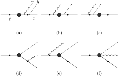
Figure 1: Feynman diagrams contributing to the decay $t\to ch\gamma$. An extra set of diagrams is obtained when the Higgs boson and the photon are exchanged. The blob represents the one-loop contributions from irreducible Feynman diagrams. In the massless charm quark limit, the diagrams in which the Higgs boson emerges from the $c$ quark give no contribution as the coupling $h\bar{c}c$ is proportional to $m_{c}$.

Figure 2: One-loop contribution to the $tc$ vertex in the unitary gauge. ${d_{i}}$ stands for a generic down quark.

Figure 3: Irreducible Feynman diagrams contributing to the $tc\gamma$ vertex in the unitary gauge.

Figure 4: The same as in Fig. 3 for the $tch$ vertex.

Figure 5: The same as in Fig. 3 for the $tch\gamma$ vertex. There is also another set of box diagrams where the Higgs boson and the photon are exchanged.

We now proceed to discuss in more detail the analytical results. We will denote the 4-momenta of the participating particles as follows

$$t(p_{1})\to c(p_{2})h(q)\gamma(k),$$ (1)

$\alpha$ stands for the photon momentum Lorentz index, and we introduce the scaled variables $x$, $y$ and $z$, given by $k\cdot p_{1}=m_{t}^{2}x/2$, $p_{1}\cdot q=m_{t}^{2}y/2$, and $p_{1}\cdot p_{2}=m_{t}^{2}z/2$, along with $\mu_{h}=m_{h}^{2}/m_{t}^{2}$. From 4-momentum conservation it follows that $z=2-x-y$. In the rest frame of the decaying $t$ quark, $x$, $y$ and $z$ are related to the energies of the final particles as follows: $x=2\,E_{\gamma}/m_{t}$, $y=2\,E_{h}/m_{t}$, and $z=2\,E_{c}/m_{t}$.

Before presenting the results, it is worth discussing the gauge invariance of the transition amplitude under $U(1)_{em}$. The calculation of the Feynman diagrams via the Passarino-Veltman reduction scheme leads to the following expression for the transition amplitude

$${\cal M}(t\to ch\gamma)=\epsilon^{*}_{\alpha}(k)\cdot\,\bar{u}_{c}(p_{2})\left({\cal M}^{\alpha}_{L}P_{L}+{\cal M}^{\alpha}_{R}P_{R}\right)u_{t}(p_{1}),$$ (2)

where $P_{L}=(1-\gamma^{5})/2$, $P_{R}=(1+\gamma^{5})/2$,

$${\cal M}^{\alpha}_{L}={A_{1}}_{L}p_{1}^{\alpha}+{A_{2}}_{L}p_{2}^{\alpha}+{A_{3}}_{L}\,\sigma^{\alpha\mu}k_{\mu}+{A_{4}}_{L}p_{1}^{\alpha}\hbox{\large$/$}\kern-5.76042pt\hbox{$k$}+{A_{5}}_{L}\gamma^{\alpha}+{A_{6}}_{L}p_{2}^{\alpha}\hbox{\large$/$}\kern-5.76042pt\hbox{$k$},$$ (3)

and a similar expression for ${\cal M}^{\alpha}_{R}$. The coefficients ${A_{i}}_{L,R}$ include the contributions of the three quarks $d_{i}$ that circulate in the loops. For this amplitude to be gauge invariant under $U(1)_{em}$, it must vanish when the polarization vector of the photon $\epsilon^{*}_{\alpha}(k)$ is replaced by its four-momentum $k_{\alpha}$, i.e., $k_{\alpha}({\cal M}_{L}^{\alpha}P_{L}+{\cal M}_{R}^{\alpha}P_{R})=0$, which is the Ward identity. One way to achieve this is that each term of the left side of the identity vanishes separately, which is equivalent to

$$(k\cdot p_{1}){A_{1}}_{L,R}+(k\cdot p_{2}){A_{2}}_{L,R}+{A_{3}}_{L,R}\,\sigma^{\alpha\mu}k_{\mu}k_{\alpha}+\left((k\cdot p_{1}){A_{4}}_{L,R}+{A_{5}}_{L,R}+(k\cdot p_{2}){A_{6}}_{L,R}\right)\hbox{\large$/$}\kern-5.76042pt\hbox{$k$}=0.$$ (4)

Since $\sigma^{\alpha\mu}k_{\mu}k_{\alpha}=0$, only the ${A_{3}}_{L,R}$ term vanishes automatically. It means that the remaining coefficients ${A_{i}}_{L,R}$ are not independent since the only way to fulfill the above equation is that $(k\cdot p_{1}){A_{1}}_{L,R}+(k\cdot p_{2}){A_{2}}_{L,R}=0$ and $(k\cdot p_{1}){A_{4}}_{L,R}+{A_{5}}_{L,R}+(k\cdot p_{2}){A_{6}}_{L,R}=0$. Therefore, if we showed that the coefficients obtained in our calculation fulfill these relations then we would have shown that the transition amplitude is gauge invariant under $U(1)_{em}$. We have verified explicitly that the amplitude obtained from our calculation obeys these relations. We can thus express ${A_{2}}_{L,R}$ in terms of ${A_{1}}_{L,R}$, whereas ${A_{5}}_{L,R}$ can be expressed in terms of ${A_{4}}_{L,R}$ and ${A_{6}}_{L,R}$. Using these results, the ${\cal M}_{L,R}$ amplitude can be rewritten in the form

$${\cal M}^{\alpha}_{L,R} = \frac{{F_{1}}_{L,R}}{m_{t}}\left((k\cdot p_{2})p_{1}^{\alpha}-(k\cdot p_{1})p_{2}^{\alpha}\right)+i\,m_{t}\,{F_{2}}_{L,R}\,\sigma^{\alpha\mu}k_{\mu}+{F_{3}}_{L,R}\left(p_{1}^{\alpha}\hbox{\large$/$}\kern-5.76042pt\hbox{$k$}-(k\cdot p_{1})\gamma^{\alpha}\right)$$ (5)

$$+ {F_{4}}_{L,R}\left(p_{2}^{\alpha}\hbox{\large$/$}\kern-5.76042pt\hbox{$k$}-(k\cdot p_{2})\gamma^{\alpha}\right).$$

where the new coefficients ${F_{i}}_{L,R}$ are given in terms of the old coefficients ${A_{i}}_{L,R}$. It is easy to see that the above equation vanishes when contracted with $k_{\alpha}$. The coefficients ${F_{i}}_{L,R}$ are too cumbersome to be presented here, we will content with presenting the results in the limit of a massless charm quark, in which case the charm quark becomes purely left-handed, namely, $u_{c}(p_{2})\to P_{L}u_{c}(p_{2})$ or $\bar{u}_{c}(p_{2})\to\bar{u}_{c}(p_{2})P_{R}$ . As a result, the ${F_{1}}_{L}$, ${F_{2}}_{L}$, ${F_{3}}_{R}$, and ${F_{4}}_{R}$ terms must vanish in this limit. We have also verified that this is true by setting $m_{c}=0$ in the general results. On the other hand, we cannot set $m_{d_{i}}=0$ since the whole amplitude would vanish when summing over the three quark families due to the GIM mechanism.

After squaring the amplitude (2) we average over initial spins and sum over final polarizations to obtain, in the $m_{c}=0$ limit:

$$|{\cal M}(t\to ch\gamma)|^{2} = \frac{m_{t}^{6}}{8}\Big{[}u\,z(x\,z-\,u)|{F_{1}}_{R}|^{2}+8\,x\,u\,|{F_{2}}_{R}|^{2}+2\,x^{2}\,z|{F_{3}}_{L}|^{2}+2\,u^{2}\,z|{F_{4}}_{L}|^{2}+4\,u\,{\rm Re}\Big{(}2\,x\,{F_{3}}_{L}{F_{2}}_{R}^{\dagger}$$ (6)

$$+ (x\,z-u)\big{(}{F_{1}}_{R}{F_{2}}_{R}^{\dagger}+{F_{3}}_{L}{F_{1}}_{R}^{\dagger}\big{)}+u\big{(}{F_{3}}_{L}{F_{4}}_{L}^{\dagger}+2\,{F_{4}}_{L}{F_{2}}_{R}^{\dagger}\big{)}\Big{)}\Big{]},$$

where we introduced the auxiliary variable $u=1+\mu_{h}-y$.

II.1 Decay width

From the square amplitude, we obtain the photon energy distribution, which is given by

$$\frac{d\Gamma(t\to ch\gamma)}{dx}=\int_{1-x+\frac{\mu_{h}}{1-x}}^{1+\mu_{h}}|{\cal M}(t\to ch\gamma)|^{2}dy,$$ (7)

whereas the decay width reads

$$\Gamma(t\to ch\gamma)=\frac{m_{t}}{256\pi^{3}}\int_{x_{min}}^{1-\mu_{h}}\frac{d\Gamma(t\to ch\gamma)}{dx}dx,$$ (8)

where $x_{min}=2{E_{\gamma}}_{min}/m_{t}$, with ${E_{\gamma}}_{min}$ being an arbitrary minimum value for the photon energy. We cannot integrate over the whole photon energy spectrum since the denominator of the amplitude coming from the Feynman diagrams where the photon emerges from the external top quark have a factor $(p_{1}-k)^{2}-m_{t}^{2}=-2k\cdot p_{1}=-2m_{t}E_{\gamma}$, which vanishes when $E_{\gamma}=0$. This is an infrared singularity which reflects the fact that a zero energy photon cannot be experimentally detected. The infrared nature of the transition amplitude can be observed in Fig. 6, where we have plotted the $t\to ch\gamma$ photon energy distribution for $m_{h}=115$ GeV.

Figure 6: Photon energy distribution for the decay $t\to ch\gamma$ in the SM and for $m_{h}=115$ GeV. The vertical scale is in units of $10^{-17}$. We have imposed a cutoff of $E_{\gamma}>1$ GeV to tame the infrared singularity.

The branching fraction follows easily after dividing (8) by the main top quark decay width $\Gamma(t\to bW)$. Using the current values for the SM parameters Eidelman:2004wy , numerical integration of Eq. (8) gives the result $Br(t\to ch\gamma)\sim 10^{-15}$ GeV for a Higgs boson mass around 115 GeV and ${E_{\gamma}}_{min}=1$ GeV. For a heavier Higgs boson the branching ratio is one order below, as shown in Fig. 7. In obtaining these numerical results, the Passarino-Veltman scalar form factors were evaluated numerically via the FF routines vanOldenborgh:1990yc . This very suppressed result is mainly due to the GIM mechanism and phase space suppression. It is somewhat interesting to assess how each single term in Eq. (6) contributes to the decay width. In Table 1 we present the partial contribution of each term appearing in Eq. (6) for $m_{h}=115$ GeV. We see that the largest contribution comes from the coefficient ${F_{1}}_{R}$, whereas the coefficient ${F_{4}}_{L}$ gives a contribution one order of magnitude below.

Figure 7: $Br(t\to ch\gamma)$ in the SM as a function of the Higgs boson mass. We consider $E_{\gamma}>1$ GeV.

Table 1: Partial contribution to the $Br(t\to ch\gamma)$ from each term in Eq. (6) for $m_{h}=115$ GeV.

	$|{F_{3}}_{L}|^{2}$	$|{F_{4}}_{L}|^{2}$	$|{F_{1}}_{R}|^{2}$	$|{F_{2}}_{R}|^{2}$	${F_{3}}_{L}{F_{2}}_{R}^{\dagger}$	${F_{1}}_{R}{F_{2}}_{R}^{\dagger}$	${F_{3}}_{L}{F_{1}}_{R}^{\dagger}$	${F_{3}}_{L}{F_{4}}_{L}^{\dagger}$	${F_{4}}_{L}{F_{2}}_{R}^{\dagger}$
Contribution$\times 10^{16}$	2.2	0.13	9.7	5.4	-4.8	2.4	-0.24	0.4	-0.9

III Decay $t\to ch\gamma$ in the THDM-III

In the THDM-III, the quarks are allowed to couple simultaneously to more than one scalar doublet Cheng:1987rs . This leaves open the possibility of sizeable effects in the scalar FCNC couplings involving quarks of the second and third generations. Unlike the first and second versions of the THDM, in model III no ad hoc symmetries are invoked to eliminate tree-level scalar FCNC couplings but instead a more realistic pattern for the Yukawa matrices is imposed and constraints on the scalar FCNC are derived from phenomenology Atwood:1996vj . The tree-level scalar FCNC interactions are given by

$${\cal{L}}_{Y,FCNC}^{III}=\xi_{ij}\sin{\alpha}\bar{f_{i}}f_{j}h+\xi_{ij}\cos{\alpha}\bar{f_{i}}f_{j}H+\xi_{ij}\cos{\alpha}\bar{f_{i}}\gamma^{5}f_{j}A+{\rm H.c.},$$ (9)

where we are using the Higgs mass-eigenstate basis with the light and heavy CP-even Higgs bosons $h$ and $H$, and the CP-odd Higgs boson $A$, $\alpha$ denotes the mixing angle, and $\xi_{ij}$ corresponds to the off-diagonal Yukawa couplings. It is usual to use the parametrization introduced by Cheng and Sher in Ref. Cheng:1987rs : $\xi_{ij}=\lambda_{ij}\sqrt{m_{i}m_{j}}/v$, where the mass factor gives the strength of the interaction, whereas the dimensionless parameters $\lambda_{ij}$ are usually assumed of order unity. Although the couplings involving light quarks are naturally suppressed according to this parametrization, the interaction $tc\phi$, with $\phi$ any of the three physical Higgs bosons of the THDM, is much less suppressed. Therefore, it is interesting to examine to what extent the decay $t\to ch\gamma$ can be enhanced by this model.

The tree-level Feynman diagrams contributing to $t\to c\phi\gamma$ are similar to those shown in Fig. 1(d) and 1(e). For illustration purposes it is enough to consider the decay into the lightest CP-even Higgs boson $h$. We will omit the factor $\sin\alpha$, which is to be reinserted when necessary. We will calculate the decay rate without neglecting the $c$ quark mass. The transition amplitude can be arranged as in Eqs. (2) and (5):

$${\cal M}^{\rm III}(t\to ch\gamma)=-\frac{i\pi\,\alpha\,\lambda_{tc}}{3\,s_{W}\,m_{W}}\frac{\sqrt{m_{t}\,m_{c}}}{k\cdot p_{1}\,k\cdot p_{2}}{\bar{u}}_{c}(p_{2})\Big{(}(k\cdot q)\,i\,\sigma^{\alpha\mu}k_{\mu}+2\left((k\cdot p_{2})p_{1}^{\alpha}-(k\cdot p_{1})p_{2}^{\alpha}\right)\Big{)}u_{t}(p_{1})\cdot\epsilon^{*}_{\alpha},$$ (10)

As discussed above, this amplitude vanishes when $\epsilon^{*}_{\alpha}$ is replaced by $k_{\alpha}$, thereby being $U(1)_{em}$ gauge invariant. The square amplitude reads

$$|{\cal M}^{\rm III}(t\to ch\gamma)|^{2} = \left(\frac{4\,\pi\,\alpha\,\lambda_{tc}}{3}\right)^{2}\frac{\sqrt{\mu_{c}}m_{t}^{2}}{2\,s_{W}^{2}\,m_{W}^{2}\,u^{2}\,x^{2}}\Big{(}u\,(u^{2}\,(2+x)+2\,(x+1)(y-2)u+x\,(x^{2}+2\,(y-2)(x+y-2)))$$ (11)

$$- 4\,u\,(u+x\,(x+y-2))\,\mu_{c}^{1/2}+2\,x^{2}\,(u+y-2)\,\mu_{c}-4\,x^{2}\,\mu_{c}^{3/2}\Big{)},$$

where $\mu_{c}=m_{c}^{2}/m_{t}^{2}$ and $u$ is now defined as $u=1+\mu_{h}-\mu_{c}-y$. This result can be inserted into Eq. (8) to obtain the $t\to ch\gamma$ branching fraction. However, the above result is also infrared divergent and we should be careful when integrating over the photon energy. Assuming and idealized situation, we will calculate the decay width in the rest frame of the $t$ quark and impose a minimum cut of $10$ GeV on the photon energy. This is equivalent to introduce a fictitious photon mass $m_{\gamma}=10$ GeV. The integration limits are thus

$$2\sqrt{\mu_{\gamma}}\leq x\leq 1+\mu_{\gamma}-\mu_{h}-\mu_{c}-2\,\sqrt{\mu_{c}\,\mu_{h}},$$ (12)

$$y_{min,\,max}=\frac{1}{2(1-x-\mu_{\gamma})}\left((2-x)(1+\mu_{\gamma}+\mu_{h}-\mu_{c}-x)\mp\sqrt{x^{2}-4\,\mu_{\gamma}}\,\lambda^{\frac{1}{2}}(1+\mu_{\gamma}-x,\mu_{h},\mu_{c})\right),$$ (13)

with $\mu_{\gamma}=m_{\gamma}^{2}/m_{t}^{2}$ and $\lambda(x,y,z)=x^{2}+y^{2}+z^{2}-2(xy+xz+yz)$. Assuming $\lambda_{tc}\sim 1$, numerical integration of Eq. (8) yields $Br(t\to ch\gamma)\sim 10^{-4}$ for $m_{h}$ around 115 GeV. In Fig. 8 we have plotted the $t\to ch\gamma$ branching ratio as a function of $m_{h}$. For $m_{h}$ ranging between 110 and 140 GeV, $Br(t\to ch\gamma)$ is of the order of $10^{-5}$, but it decreases quickly as $m_{h}$ approaches the top quark mass.

Figure 8: $t\to ch\gamma$ branching ratio in the THDM-III as a function of the Higgs boson mass. We assumed $E_{\gamma}\geq 10$ GeV and $\lambda_{tc}\sim 1$.

III.1 The decay $h\to b\bar{s}\gamma$

It is also interesting to consider the crossed decay $h\to b\bar{s}\gamma$, which is also very suppressed in the SM. The two-body decay $h\to b\bar{s}$ has already been calculated in the SM Haeri , the THDM Arhrib:2004xu , and the MSSM Bejar:2004rz . It has been found that this decay mode may be at the reach of future colliders. In the THDM-II, the two-body decay $h\to b{\bar{s}}$ as well as the $h\to b{\bar{s}}\gamma$ one are suppressed by a factor $\sqrt{m_{b}m_{s}}$, which enters into the Cheng-Sher ansatz for the $Hb\bar{s}$ coupling. The numerical calculation yields the $h\to b{\bar{s}}\gamma$ branching ratio shown in Fig. 9 as a function of $m_{h}$. We assumed that the total decay width of the Higgs boson is approximately the SM one, which was calculated via the HDECAY program Djouadi:1997yw . For 115 GeV $\leq m_{h}\leq$ 130 GeV the main decay channel of the Higgs boson is $h\to b\bar{b}$. Around $m_{h}=130$ GeV, the channel $h\to WW^{*}$ becomes more important, and for $m_{h}\geq 2\,m_{W}$ the $h\to WW$ mode, with two $W$ real, becomes the main decay channel. So the $h\to b{\bar{s}}\gamma$ decay start to decrease dramatically for $m_{h}$ around 140 GeV.

Figure 9: $h\to b\bar{s}\gamma$ branching ratio in the THDM-III as a function of the Higgs boson mass. We assumed $E_{\gamma}\geq 10$ GeV and $\lambda_{bs}\sim 1$.

IV conclusion

Although the top quark can have a wide spectrum of decay modes due to its large mass, it has a very restrictive dynamical behavior according to the SM predictions. This means that this particle may be very sensitive to new physics effects, which is strongly suggested by several SM extensions, which predict sizeable branching ratios for some rare top quark decay modes. In this paper we have presented an explicit calculation of the decay $t\to ch\gamma$ both in the SM and the THDM-III. As occurs with the FCNC two-body decay $t\to ch$, the three-body decay $t\to ch\gamma$ is negligibly small in the SM due to the GIM mechanism and phase space suppression. The reason why the decay width is so small even if there are infrared singularities is because the GIM mechanism strongly suppresses those loops diagrams carrying down quarks. In contrast, in the THDM-III the decay $t\to ch\gamma$ can be dramatically enhanced in part due to the existence of tree-level scalar FCNCs but also because of infrared singularities. In this model the $t\to ch\gamma$ branching ratio can be up to ten orders of magnitude larger than in the SM. So it can be an alternative mode to search for FCNC effects. Notice that in order to tame the infrared singularities, we integrate the decay width imposing a cut off on the photon energy. Although we calculate the decay width in the SM using a minimum photon energy of 1 GeV, the result is still strongly suppressed, whereas in the THDM there is a dramatic enhancement even if we use a cut off of 10 GeV.

As far as the crossed decay $h\to d_{i}\bar{u_{j}}\gamma$ is concerned, this is also very suppressed in the SM. In the THDM-III, the $h\to d_{i}\bar{u_{j}}\gamma$ branching ratio is proportional to $m_{d_{i}}\,m_{u_{j}}$, so it gets somewhat suppressed for external light quarks. In particular, $Br(h\to b\bar{s}\gamma)\sim 10^{-5}$ for $m_{h}\sim 115$ GeV, but it decreases dramatically for a heavier Higgs boson as more decay channels get opened.

Appendix A Amplitudes for the SM decay $t\to ch\gamma$

In this appendix we present the amplitudes for the decay $t\to ch\gamma$ in terms of Passarino-Veltman form factors Passarino:1978jh . We split the total amplitude into five pieces. The ${F_{i}}_{L,R}$ coefficients arising from the $tc$ vertex plus the $tc\gamma$ one will be denoted by the superscript $tc+tc\gamma$, whereas $tch$ will denote those contributions arising from the irreducible $tch$ vertex alone. As for the box diagrams, $\rm Box_{1}$, $\rm Box_{2}$, and $\rm Box_{3}$ will denote the contributions from the box diagrams with one, two and three internal $W$ gauge bosons, respectively. As discussed in Sec. II, the contribution denoted by the superscript $tc+tc\gamma$ is ultraviolet finite by itself, whereas the remaining contributions, $tch$ and ${\rm Box}_{i}$, give an ultraviolet finite amplitude by its own, but they should be added together to obtain gauge invariance. We do not present below any non gauge invariant terms since they cancel each other when adding the whole contributions.

Each coefficient will be written as

$${F_{i}}_{L,R}=\frac{\alpha^{2}}{2\,s_{W}^{3}\,m_{W}}\sum_{d_{i}=d,\,s,\,b}V_{td_{i}}V^{\dagger}_{d_{i}c}\left({G_{i}}_{L,R}^{tc+tc\gamma}+{G_{i}}_{L,R}^{tch}+\sum_{i=1}^{3}{G_{i}}_{L,R}^{{\rm Box}_{i}}\right).$$ (14)

The quark color factor is already included and we also introduced explicitly the values of the quark charges. The nonzero coefficients ${G_{i}}_{L,R}^{tc+tc\gamma}$ are given by

$${G_{4}}_{L}^{tc+tc\gamma} = \frac{1}{\eta m_{W}^{2}}\Bigg{[}um_{t}^{2}\Big{(}3(C_{0}^{(1)}+C_{1}^{(1)}+C_{2}^{(1)}-C_{2}^{(22)}+C_{11}^{(1)}+2C_{1}^{(22)}+3C_{12}^{(1)}+2C_{22}^{(1)})+2(C_{2}^{(13)}+C_{11}^{(21)})+C_{0}^{(2)}$$ (15)

$$+ C_{1}^{(13)}+C_{1}^{(21)}+C_{12}^{(21)}\Big{)}-m_{d_{i}}^{2}\Big{(}C_{1}^{(21)}+3(C_{1}^{(22)}+C_{12}^{(1)}+C_{22}^{(1)}+C_{12}^{(21)})+C_{11}^{(21)}\Big{)}-m_{W}^{2}\Big{(}3(C_{0}^{(1)}-C_{1}^{(1)}$$

$$- C_{2}^{(1)}+C_{12}^{(1)}+C_{22}^{(1)}+2C_{1}^{(22)})+C_{0}^{(2)}+C_{1}^{(21)}+2(C_{11}^{(21)}-C_{12}^{(21)})\Big{)}+6C_{00}^{(1)}+3C_{00}^{(21)}-B_{0}^{(1)}-B_{0}^{(2)}\Bigg{]},$$

$${G_{1}}_{R}^{tc+tc\gamma} = \frac{1}{2\eta m_{W}^{2}}\Bigg{[}\frac{m_{d_{i}}^{2}}{m_{t}^{2}}\Big{(}2(1+B_{0}^{(1)}+2C_{00}^{(21)}+3C_{00}^{(1)})-5B_{0}^{(2)}+B_{0}^{(7)}\Big{)}-u\Big{(}B_{0}^{(1)}-B_{0}^{(2)}\Big{)}-um_{d_{i}}^{2}C_{2}^{(13)}$$ (16)

$$+ \frac{\left({m_{W}^{2}}+m_{d_{i}}^{2}\right)m_{d_{i}}^{2}-2m_{W}^{4}}{um_{t}^{4}}\Big{(}B_{0}^{(2)}-B_{0}^{(7)}\Big{)}-\frac{2m_{W}^{2}}{m_{t}^{2}}\Big{(}1+2(B_{0}^{(2)}-3C_{00}^{(1)}-C_{00}^{(21)})+B_{0}^{(3)}-B_{0}^{(7)}\Big{)}$$

$$+ u^{2}m_{t}^{2}\Big{(}C_{0}^{(2)}+C_{1}^{(13)}+2C_{2}^{(13)}\Big{)}-um_{W}^{2}\Big{(}C_{0}^{(2)}+2(3(C_{0}^{(1)}+2C_{1}^{(22)}+2C_{2}^{(22)})+C_{2}^{(13)})\Big{)}\Bigg{]},$$

where $\xi=1-x$ and $\eta=1-u$. $B_{0}^{(i)}$, $C_{0}^{(i)}$, and $D_{0}^{(i)}$ are Passarino-Veltman scalar functions Passarino:1978jh , whereas $C_{lm}^{(i)}$ and $D_{lm}^{(i)}$ stand for the coefficient functions of tensor integrals. We follow the same nomenclature introduced in Mertig:1990an . The arguments of the Passarino-Veltman functions are represented by the superscript $(i)$ and are presented in Tables 2, 3, and 4. Note that although the $C_{0}$ and $D_{0}$ scalar functions are invariant under the permutation of their arguments, this is not true in general for the coefficient functions $C_{lm}$ and $D_{lm}$.

Table 2: Arguments for the two-point Passarino-Veltman scalar functions: $B_{0}^{(i)}=B_{0}(1,2,3)$. According to our notation $(p_{1}-k)^{2}=m_{t}^{2}(1-x)$, $(p_{1}-p_{2})^{2}=m_{h}^{2}+m_{t}^{2}\,(x-u)$, and $(p_{1}-q)^{2}=m_{t}^{2}\,u$.

$(i)$	1	2	3
$(1)$	$0$	$m_{d_{i}}^{2}$	$m_{d_{i}}^{2}$
$(2)$	$0$	$m_{d_{i}}^{2}$	$m_{W}^{2}$
$(3)$	$0$	$m_{W}^{2}$	$m_{W}^{2}$
$(4)$	$m_{h}^{2}$	$m_{d_{i}}^{2}$	$m_{d_{i}}^{2}$
$(5)$	$m_{h}^{2}$	$m_{W}^{2}$	$m_{W}^{2}$
$(6)$	$m_{t}^{2}$	$m_{d_{i}}^{2}$	$m_{W}^{2}$
$(7)$	$(p_{1}-q)^{2}$	$m_{d_{i}}^{2}$	$m_{W}^{2}$
$(8)$	$(p_{1}-k)^{2}$	$m_{d_{i}}^{2}$	$m_{W}^{2}$
$(9)$	$(p_{1}-p_{2})^{2}$	$m_{d_{i}}^{2}$	$m_{d_{i}}^{2}$
$(10)$	$(p_{1}-p_{2})^{2}$	$m_{W}^{2}$	$m_{W}^{2}$

Table 3: Arguments for the three-point Passarino-Veltman coefficient functions: $C_{lm}^{(i)}=C_{lm}(1,2,3,4,5,6)$.

$(i)$	1	2	3	4	5	6
$(1)$	$0$	$0$	$(p_{1}-q)^{2}$	$m_{d_{i}}^{2}$	$m_{W}^{2}$	$m_{W}^{2}$
$(2)$	$0$	$0$	$(p_{1}-q)^{2}$	$m_{W}^{2}$	$m_{d_{i}}^{2}$	$m_{d_{i}}^{2}$
$(3)$	$0$	$m_{h}^{2}$	$(p_{1}-k)^{2}$	$m_{d_{i}}^{2}$	$m_{W}^{2}$	$m_{W}^{2}$
$(4)$	$0$	$m_{h}^{2}$	$(p_{1}-k)^{2}$	$m_{W}^{2}$	$m_{d_{i}}^{2}$	$m_{d_{i}}^{2}$
$(5)$	$0$	$m_{h}^{2}$	$(p_{1}-p_{2})^{2}$	$m_{d_{i}}^{2}$	$m_{d_{i}}^{2}$	$m_{d_{i}}^{2}$
$(6)$	$0$	$m_{h}^{2}$	$(p_{1}-p_{2})^{2}$	$m_{W}^{2}$	$m_{W}^{2}$	$m_{W}^{2}$
$(7)$	$m_{t}^{2}$	$0$	$(p_{1}-k)^{2}$	$m_{d_{i}}^{2}$	$m_{W}^{2}$	$m_{W}^{2}$
$(8)$	$m_{t}^{2}$	$0$	$(p_{1}-k)^{2}$	$m_{W}^{2}$	$m_{d_{i}}^{2}$	$m_{d_{i}}^{2}$
$(9)$	$m_{t}^{2}$	$m_{h}^{2}$	$(p_{1}-q)^{2}$	$m_{d_{i}}^{2}$	$m_{W}^{2}$	$m_{W}^{2}$
$(10)$	$m_{t}^{2}$	$m_{h}^{2}$	$(p_{1}-q)^{2}$	$m_{W}^{2}$	$m_{d_{i}}^{2}$	$m_{d_{i}}^{2}$
$(11)$	$m_{t}^{2}$	$(p_{1}-p_{2})^{2}$	$0$	$m_{d_{i}}^{2}$	$m_{W}^{2}$	$m_{W}^{2}$
$(12)$	$m_{t}^{2}$	$(p_{1}-p_{2})^{2}$	$0$	$m_{W}^{2}$	$m_{d_{i}}^{2}$	$m_{d_{i}}^{2}$
$(13)$	$0$	$0$	$(p_{1}-q)^{2}$	$m_{d_{i}}^{2}$	$m_{d_{i}}^{2}$	$m_{W}^{2}$
$(14)$	$0$	$(p_{1}-k)^{2}$	$m_{t}^{2}$	$m_{d_{i}}^{2}$	$m_{d_{i}}^{2}$	$m_{W}^{2}$
$(15)$	$m_{h}^{2}$	$0$	$(p_{1}-k)^{2}$	$m_{d_{i}}^{2}$	$m_{d_{i}}^{2}$	$m_{W}^{2}$
$(16)$	$m_{h}^{2}$	$0$	$(p_{1}-p_{2})^{2}$	$m_{d_{i}}^{2}$	$m_{d_{i}}^{2}$	$m_{d_{i}}^{2}$
$(17)$	$m_{h}^{2}$	$(p_{1}-q)^{2}$	$m_{t}^{2}$	$m_{d_{i}}^{2}$	$m_{d_{i}}^{2}$	$m_{W}^{2}$
$(18)$	$m_{t}^{2}$	$0$	$(p_{1}-p_{2})^{2}$	$m_{d_{i}}^{2}$	$m_{W}^{2}$	$m_{d_{i}}^{2}$
$(19)$	$m_{t}^{2}$	$(p_{1}-q)^{2}$	$m_{h}^{2}$	$m_{d_{i}}^{2}$	$m_{W}^{2}$	$m_{d_{i}}^{2}$
$(20)$	$m_{t}^{2}$	$(p_{1}-k)^{2}$	$0$	$m_{d_{i}}^{2}$	$m_{W}^{2}$	$m_{d_{i}}^{2}$
$(21)$	$(p_{1}-q)^{2}$	$0$	$0$	$m_{d_{i}}^{2}$	$m_{W}^{2}$	$m_{d_{i}}^{2}$
$(22)$	$(p_{1}-q)^{2}$	$0$	$0$	$m_{d_{i}}^{2}$	$m_{W}^{2}$	$m_{W}^{2}$
$(23)$	$(p_{1}-q)^{2}$	$m_{h}^{2}$	$m_{t}^{2}$	$m_{d_{i}}^{2}$	$m_{W}^{2}$	$m_{W}^{2}$
$(24)$	$(p_{1}-k)^{2}$	$0$	$m_{h}^{2}$	$m_{d_{i}}^{2}$	$m_{W}^{2}$	$m_{d_{i}}^{2}$
$(25)$	$(p_{1}-k)^{2}$	$0$	$m_{t}^{2}$	$m_{d_{i}}^{2}$	$m_{W}^{2}$	$m_{W}^{2}$
$(26)$	$(p_{1}-k)^{2}$	$m_{h}^{2}$	$0$	$m_{d_{i}}^{2}$	$m_{W}^{2}$	$m_{W}^{2}$
$(27)$	$0$	$(p_{1}-q)^{2}$	$0$	$m_{d_{i}}^{2}$	$m_{d_{i}}^{2}$	$m_{W}^{2}$
$(28)$	$0$	$(p_{1}-k)^{2}$	$m_{h}^{2}$	$m_{d_{i}}^{2}$	$m_{W}^{2}$	$m_{d_{i}}^{2}$

Table 4: Arguments for the four-point Passarino-Veltman coefficient functions: $D_{lm}^{(i)}=D_{lm}(1,2,3,4,5,6,7,8,9,10)$.

$(i)$	1	2	3	4	5	6	7	8	9	10
$(1)$	$0$	$(p_{1}-k)^{2}$	$m_{h}^{2}$	$(p_{1}-q)^{2}$	$m_{t}^{2}$	$0$	$m_{W}^{2}$	$m_{W}^{2}$	$m_{d_{i}}^{2}$	$m_{d_{i}}^{2}$
$(2)$	$m_{h}^{2}$	$(p_{1}-q)^{2}$	$0$	$(p_{1}-k)^{2}$	$m_{t}^{2}$	$0$	$m_{W}^{2}$	$m_{W}^{2}$	$m_{d_{i}}^{2}$	$m_{d_{i}}^{2}$
$(3)$	$m_{t}^{2}$	$0$	$0$	$m_{h}^{2}$	$(p_{1}-p_{2})^{2}$	$(p_{1}-q)^{2}$	$m_{d_{i}}^{2}$	$m_{W}^{2}$	$m_{d_{i}}^{2}$	$m_{d_{i}}^{2}$
$(4)$	$m_{t}^{2}$	$0$	$m_{h}^{2}$	$0$	$(p_{1}-p_{2})^{2}$	$(p_{1}-k)^{2}$	$m_{d_{i}}^{2}$	$m_{W}^{2}$	$m_{d_{i}}^{2}$	$m_{d_{i}}^{2}$
$(5)$	$(p_{1}-p_{2})^{2}$	$0$	$(p_{1}-k)^{2}$	$0$	$m_{t}^{2}$	$m_{h}^{2}$	$m_{W}^{2}$	$m_{W}^{2}$	$m_{d_{i}}^{2}$	$m_{W}^{2}$
$(6)$	$(p_{1}-p_{2})^{2}$	$m_{t}^{2}$	$(p_{1}-q)^{2}$	$0$	$0$	$m_{h}^{2}$	$m_{W}^{2}$	$m_{W}^{2}$	$m_{d_{i}}^{2}$	$m_{W}^{2}$

The remaining nonzero coefficients are:

$${G_{2}}_{R}^{tch} = \frac{1}{x}\Bigg{[}2\left(2\xi-\mu_{h}\right)C_{0}^{(3)}+\frac{2m_{d_{i}}^{2}}{m_{t}^{2}m_{W}^{2}}\Big{(}1+B_{0}^{(1)}-B_{0}^{(4)}\Big{)}-2\left(\frac{m_{d_{i}}^{2}\mu_{h}}{m_{W}^{2}}-\frac{4m_{W}^{2}}{m_{t}^{2}}-\frac{m_{h}^{2}}{m_{W}^{2}}\left(\xi-{\mu_{h}}\right)+2\mu_{h}\right)C_{1}^{(26)}$$ (17)

$$- 2\frac{m_{d_{i}}^{2}}{m_{W}^{2}}\left(\frac{2m_{d_{i}}^{2}}{m_{t}^{2}}-\xi\right)\Big{(}C_{0}^{(4)}+C_{1}^{(15)}+C_{2}^{(15)}\Big{)}-\frac{2m_{d_{i}}^{2}}{m_{t}^{2}}\Big{(}2C_{0}^{(3)}+3C_{0}^{(4)}+4C_{1}^{(15)}+2C_{1}^{(26)}+4C_{2}^{(15)}\Big{)}$$

$$- \frac{2}{m_{t}^{2}}\Big{(}B_{0}^{(2)}+\ B_{0}^{(5)}-2B_{0}^{(8)}\Big{)}+\frac{m_{h}^{2}}{m_{t}^{2}m_{W}^{2}}\Big{(}B_{0}^{(5)}-2B_{0}^{(8)}\Big{)}\Bigg{]},$$

$${G_{1}}_{R}^{tch} = \frac{1}{uxm_{W}^{2}}\Bigg{[}\frac{m_{h}^{2}}{2m_{t}^{2}}\Big{(}x(B_{0}^{(5)}-2B_{0}^{(6)})+u(2B_{0}^{(8)}-B_{0}^{(5)})\Big{)}+\frac{1}{2}xuB_{0}^{(7)}+\frac{m_{d_{i}}^{2}}{2m_{t}^{2}}\Big{(}2(x-u)(1+B_{0}^{(1)}-B_{0}^{(4)})$$ (18)

$$+ x(B_{0}^{(7)}-B_{0}^{(2)})\Big{)}-\frac{m_{d_{i}}^{2}m_{h}^{2}}{m_{t}^{2}}\Big{(}u(C_{0}^{(4)}+C_{1}^{(15)}+C_{2}^{(15)}-C_{1}^{(26)})-x(C_{0}^{(10)}+C_{1}^{(17)}+C_{2}^{(17)}-C_{1}^{(9)})\Big{)}$$

$$+ \frac{2m_{d_{i}}^{4}}{m_{t}^{2}}\Big{(}u(C_{0}^{(4)}+C_{1}^{(15)}+C_{2}^{(15)})-x(C_{0}^{(10)}+C_{1}^{(17)}+C_{2}^{(17)})\Big{)}+m_{h}^{2}\Big{(}xC_{1}^{(9)}-\mu_{h}(xC_{1}^{(9)}-uC_{1}^{(26)})$$

$$- u(C_{1}^{(26)}-x(C_{0}^{(9)}+C_{1}^{(9)}+C_{1}^{(26)}+C_{2}^{(9)}))\Big{)}+m_{d_{i}}^{2}\Big{(}x(C_{0}^{(10)}+C_{1}^{(17)}+C_{2}^{(17)})-u(C_{1}^{(15)}+C_{2}^{(15)}$$

$$+ \xi C_{0}^{(4)}-x(C_{0}^{(10)}+C_{1}^{(17)}+C_{2}^{(15)}+C_{2}^{(17)}-C_{1}^{(15)}))\Big{)}+2m_{W}^{2}\Big{(}xC_{0}^{(9)}-u\xi C_{0}^{(3)}-ux(C_{0}^{(9)}+C_{2}^{(9)})\Big{)}$$

$$+ \frac{m_{W}^{2}}{2m_{t}^{2}}\Big{(}x(B_{0}^{(2)}-3B_{0}^{(7)}-2(B_{0}^{(5)}-2B_{0}^{(6)}))+2u(B_{0}^{(2)}+B_{0}^{(5)}-2B_{0}^{(8)})\Big{)}+\frac{4m_{W}^{4}}{m_{t}^{2}}\Big{(}uC_{1}^{(26)}-xC_{1}^{(9)}\Big{)}$$

$$- \frac{m_{h}^{2}m_{W}^{2}}{m_{t}^{2}}\Big{(}x(C_{0}^{(9)}-2(C_{1}^{(9)}-2C_{2}^{(9)}))-u(C_{0}^{(3)}+2(2C_{2}^{(26)}-C_{1}^{(26)}))\Big{)}+\frac{m_{d_{i}}^{2}m_{W}^{2}}{m_{t}^{2}}\Big{(}u(3C_{0}^{(4)}$$

$$+ 2(C_{0}^{(3)}+C_{1}^{(26)}+2(C_{1}^{(15)}+C_{2}^{(15)})))-x(3C_{0}^{(10)}+2(C_{0}^{(9)}-C_{1}^{(9)}+2(C_{1}^{(17)}+C_{2}^{(17)})))\Big{)}\Bigg{]},$$

$${G_{3}}_{L}^{\rm Box_{1}} = \frac{m_{d_{i}}^{2}}{m_{W}^{2}}\Bigg{[}\Big{(}C_{1}^{(14)}+C_{12}^{(14)}-C_{0}^{(4)}-C_{0}^{(8)}-C_{1}^{(16)}-C_{1}^{(20)}-C_{1}^{(24)}-C_{2}^{(5)}-C_{2}^{(16)}-C_{2}^{(20)}-C_{2}^{(24)}\Big{)}$$ (19)

$$+ m_{h}^{2}\Big{(}D_{0}^{(3)}+D_{0}^{(4)}+2(D_{1}^{(3)}+D_{12}^{(3)}+D_{12}^{(4)}+D_{2}^{(3)}+D_{2}^{(4)}-D_{13}^{(3)}+D_{3}^{(3)}+D_{23}^{(3)})+D_{22}^{(3)}+D_{22}^{(4)}+D_{33}^{(3)}\Big{)}$$

$$- 2m_{d_{i}}^{2}\Big{(}D_{0}^{(3)}+D_{0}^{(4)}+D_{1}^{(3)}+D_{1}^{(4)}+D_{2}^{(3)}+D_{2}^{(4)}+D_{13}^{(3)}+D_{33}^{(3)}-D_{13}^{(4)}-D_{23}^{(3)}-D_{23}^{(4)}+2D_{3}^{(3)}\Big{)}$$

$$- m_{t}^{2}\Big{(}D_{0}^{(3)}+D_{13}^{(4)}+D_{23}^{(4)}+D_{33}^{(3)}+2(D_{3}^{(3)}+D_{11}^{(3)}+D_{11}^{(4)}+D_{22}^{(3)}+D_{22}^{(4)}+2(D_{12}^{(3)}+D_{12}^{(4)}))+3(D_{1}^{(3)}+D_{1}^{(4)}$$

$$+ D_{2}^{(3)}+D_{2}^{(4)}+D_{13}^{(3)}+D_{23}^{(3)})+(u+\xi)D_{0}^{(4)}-x(D_{1}^{(4)}-D_{2}^{(4)})+u(D_{1}^{(3)}+D_{2}^{(4)}+D_{3}^{(4)}+D_{11}^{(4)}+D_{12}^{(3)}+D_{12}^{(4)}$$

$$+ D_{13}^{(4)}+D_{23}^{(4)}-D_{3}^{(3)}-D_{11}^{(3)}-D_{23}^{(3)}-D_{33}^{(3)}+2D_{1}^{(4)})\Big{)}+m_{W}^{2}\Big{(}D_{0}^{(3)}+D_{0}^{(4)}-D_{3}^{(3)}+3(D_{1}^{(3)}+D_{1}^{(4)}+D_{2}^{(3)}$$

$$+ D_{2}^{(4)})-4(D_{13}^{(3)}+D_{23}^{(3)}+D_{33}^{(3)}-D_{13}^{(4)}-D_{23}^{(4)})\Big{)}\Bigg{]},$$

$${G_{4}}_{L}^{\rm Box_{1}} = \frac{m_{d_{i}}^{2}}{m_{W}^{2}}\Bigg{[}C_{1}^{(16)}+C_{2}^{(5)}+C_{2}^{(16)}+C_{2}^{(24)}-C_{12}^{(27)}+2(C_{0}^{(5)}-D_{00}^{(3)}-D_{00}^{(4)})-m_{h}^{2}\Big{(}D_{3}^{(3)}+D_{22}^{(3)}$$ (20)

$$+ D_{22}^{(4)}+D_{33}^{(3)}+3D_{23}^{(3)}\Big{)}+2m_{d_{i}}^{2}\Big{(}D_{3}^{(3)}+D_{23}^{(3)}+D_{33}^{(3)}+D_{23}^{(4)}\Big{)}+m_{t}^{2}\Big{(}D_{3}^{(3)}+D_{23}^{(4)}+D_{33}^{(3)}$$

$$+ 3D_{23}^{(3)}+2(D_{2}^{(3)}+D_{12}^{(4)}+D_{13}^{(3)}+D_{22}^{(4)}-D_{22}^{(3)})+(2+u-x)D_{2}^{(4)}+(2+u)D_{12}^{(3)}$$

$$+ u(D_{12}^{(4)}+D_{13}^{(3)}+D_{23}^{(4)}-D_{23}^{(3)}-D_{33}^{(3)})-\mu_{h}(D_{2}^{(3)}+D_{2}^{(4)}+D_{12}^{(3)}+D_{12}^{(4)}-D_{13}^{(3)}-D_{23}^{(3)})\Big{)}$$

$$+ m_{W}^{2}\Big{(}D_{2}^{(3)}+D_{2}^{(4)}+5D_{3}^{(3)}+2(D_{0}^{(3)}+D_{0}^{(4)}+2(D_{23}^{(3)}+D_{33}^{(3)}-D_{23}^{(4)}))\Big{)}\Bigg{]},$$

$${G_{2}}_{R}^{\rm Box_{1}} = -\frac{m_{d_{i}}^{2}}{m_{W}^{2}}\Bigg{[}C_{0}^{(4)}+C_{0}^{(5)}+C_{1}^{(16)}+C_{1}^{(20)}+C_{1}^{(24)}+C_{2}^{(5)}+C_{2}^{(16)}+C_{2}^{(24)}+C_{22}^{(14)}-2C_{2}^{(14)}-2m_{d_{i}}^{2}\Big{(}D_{0}^{(3)}+D_{1}^{(4)}$$ (21)

$$+ D_{2}^{(4)}+D_{11}^{(3)}+D_{11}^{(4)}+D_{22}^{(3)}+D_{22}^{(4)}+D_{33}^{(3)}+2(D_{1}^{(3)}+D_{2}^{(3)}+D_{3}^{(3)}+D_{12}^{(4)}+D_{13}^{(3)}+D_{23}^{(3)}-D_{12}^{(3)})\Big{)}$$

$$- m_{W}^{2}\Big{(}3(D_{0}^{(3)}+D_{1}^{(4)}+D_{2}^{(4)})+7(D_{1}^{(3)}+D_{2}^{(3)}+D_{3}^{(3)})+4(D_{11}^{(3)}+D_{22}^{(3)}+D_{22}^{(4)}-D_{11}^{(4)}-D_{33}^{(3)}+2(D_{12}^{(3)}$$

$$+ D_{12}^{(4)}+D_{13}^{(3)}+D_{23}^{(3)}))\Big{)}+m_{t}^{2}\Big{(}D_{0}^{(3)}+D_{1}^{(4)}+D_{11}^{(3)}+D_{11}^{(4)}+D_{22}^{(3)}+D_{22}^{(4)}+D_{33}^{(3)}+2(D_{1}^{(3)}+D_{3}^{(3)}+D_{12}^{(3)}$$

$$+ D_{12}^{(4)}+D_{13}^{(3)}+D_{23}^{(3)})+\eta D_{2}^{(4)}-(u-2)D_{2}^{(3)}-u(D_{3}^{(3)}+D_{12}^{(3)}+D_{12}^{(4)}+D_{13}^{(3)}+D_{22}^{(3)}+D_{22}^{(4)}+D_{33}^{(3)}$$

$$- 2D_{23}^{(3)})\Big{)}-4m_{h}^{2}D_{2}^{(3)}\Bigg{]},$$

$${G_{1}}_{R}^{\rm Box_{1}} = \frac{m_{d_{i}}^{2}}{2m_{W}^{2}}\Bigg{[}C_{0}^{(8)}+C_{0}^{(10)}+C_{1}^{(20)}+C_{2}^{(17)}+2(C_{0}^{(5)}+C_{1}^{(17)}-D_{00}^{(3)}-D_{00}^{(4)})-2m_{h}^{2}D_{0}^{(4)}$$ (22)

$$+ (2m_{d_{i}}^{2}-m_{t}^{2})\Big{(}D_{0}^{(3)}+D_{0}^{(4)}+D_{1}^{(3)}+D_{1}^{(4)}+D_{2}^{(3)}+D_{2}^{(4)}+D_{3}^{(3)}\Big{)}+m_{t}^{2}\Big{(}uD_{3}^{(3)}-xD_{3}^{(4)}\Big{)}$$

$$- m_{W}^{2}\Big{(}D_{0}^{(3)}+D_{0}^{(4)}+4(D_{1}^{(3)}+D_{1}^{(4)}+D_{2}^{(3)}+D_{2}^{(4)}+D_{3}^{(3)})\Big{)}\Bigg{]},$$

$${G_{3}}_{L}^{\rm Box_{2}} = -\frac{m_{d_{i}}^{2}}{2m_{W}^{2}}\Bigg{[}2(C_{1}^{(14)}+C_{2}^{(14)}+C_{12}^{(14)}-C_{1}^{(20)}-C_{2}^{(20)}-3(C_{1}^{(19)}+C_{2}^{(25)}+C_{12}^{(25)}+D_{00}^{(1)}-2C_{1}^{(25)}))$$ (23)

$$+ 3(C_{2}^{(19)}+C_{2}^{(28)}-C_{0}^{(10)}+2(C_{0}^{(7)}+C_{11}^{(25)}))+m_{t}^{2}\Big{(}3((x-2(u+1))D_{2}^{(1)}+(x-2)(D_{12}^{(1)}+D_{23}^{(1)}$$

$$+ 2D_{22}^{(1)})+u(D_{3}^{(1)}+D_{13}^{(1)}+D_{33}^{(1)}-2(D_{12}^{(1)}+D_{22}^{(1)}+D_{23}^{(1)})))-\mu_{h}(D_{1}^{(2)}+D_{3}^{(2)}+D_{11}^{(2)}$$

$$+ D_{23}^{(2)}+D_{33}^{(2)}-D_{12}^{(2)}+2D_{13}^{(2)}-3(D_{22}^{(1)}-D_{1}^{(1)}))\Big{)}+12m_{d_{i}}^{2}\Big{(}D_{2}^{(1)}+D_{12}^{(1)}+D_{23}^{(1)}\Big{)}\Bigg{]}+C_{2}^{(14)}-C_{1}^{(9)}$$

$$- 2m_{t}^{2}\Big{(}D_{11}^{(2)}+D_{33}^{(2)}+2(D_{3}^{(2)}+D_{13}^{(2)}+D_{22}^{(2)})+3(D_{2}^{(2)}+D_{12}^{(2)}+D_{23}^{(2)})+\xi(D_{0}^{(2)}+2D_{1}^{(2)})$$

$$+ u(D_{2}^{(2)}+D_{12}^{(2)}+D_{22}^{(2)}+D_{23}^{(2)})-x(D_{11}^{(2)}+D_{33}^{(2)}-D_{22}^{(2)}+2(D_{2}^{(2)}+D_{3}^{(2)}+D_{12}^{(2)}+D_{13}^{(2)}+D_{23}^{(2)}))$$

$$- \mu_{h}(D_{0}^{(2)}+D_{11}^{(2)}+D_{22}^{(2)}+D_{33}^{(2)}+2(D_{1}^{(2)}+D_{2}^{(2)}+D_{12}^{(2)}+D_{13}^{(2)}+D_{23}^{(2)}-D_{3}^{(2)}))\Big{)}$$

$$- 2m_{W}^{2}\Big{(}2(D_{11}^{(2)}+D_{12}^{(2)}+D_{33}^{(2)}-D_{23}^{(2)}+2D_{13}^{(2)})+3(D_{0}^{(2)}+D_{2}^{(2)})+5(D_{1}^{(2)}+D_{3}^{(2)})\Big{)}$$

$$+ 2m_{d_{i}}^{2}\Big{(}2(D_{2}^{(2)}-D_{11}^{(2)}-D_{12}^{(2)}-D_{23}^{(2)}-D_{33}^{(2)}-2(D_{13}^{(2)}-3(D_{12}^{(1)}+D_{23}^{(1)})))-3(2D_{0}^{(1)}+3D_{2}^{(1)})\Big{)},$$

$${G_{4}}_{L}^{\rm Box_{2}} = \frac{m_{d_{i}}^{2}}{2m_{W}^{2}}\Bigg{[}3(C_{0}^{(4)}+C_{2}^{(28)}-C_{2}^{(19)}+2(C_{2}^{(1)}+C_{12}^{(1)}+C_{22}^{(1)}-3D_{00}^{(1)}))-2(C_{2}^{(13)}+C_{12}^{(13)}+C_{22}^{(13)})$$ (24)

$$+ 12m_{d_{i}}^{2}\Big{(}D_{3}^{(1)}+D_{13}^{(1)}+D_{33}^{(1)}\Big{)}+2m_{W}^{2}\Big{(}2(D_{11}^{(2)}+D_{13}^{(2)}+6(D_{13}^{(1)}+D_{33}^{(1)}))+3(2D_{0}^{(1)}+5D_{3}^{(1)})\Big{)}$$

$$- m_{t}^{2}\Big{(}3(2(1+u)D_{3}^{(1)}+(2+3u)(D_{13}^{(1)}+D_{33}^{(1)})+xD_{12}^{(1)}+(2(2+u)-x)D_{23}^{(1)})-2\mu_{h}(D_{1}^{(2)}+D_{11}^{(2)}$$

$$+ D_{13}^{(2)}+3(D_{23}^{(1)}-2D_{13}^{(1)}))\Big{)}\Bigg{]}+2m_{t}^{2}\Big{(}D_{2}^{(2)}+D_{3}^{(2)}+D_{11}^{(2)}+D_{13}^{(2)}+2D_{12}^{(2)}+\xi(D_{0}^{(2)}+2D_{1}^{(2)})$$

$$+ u(D_{2}^{(2)}+D_{12}^{(2)})-x(D_{2}^{(2)}+D_{3}^{(2)}+D_{11}^{(2)}+D_{12}^{(2)}+D_{13}^{(2)})+{\mu_{h}}(D_{0}^{(2)}+D_{2}^{(2)}+D_{3}^{(2)}+D_{11}^{(2)}+D_{12}^{(2)}$$

$$+ D_{13}^{(2)}+2D_{1}^{(2)})\Big{)}+2m_{W}^{2}\Big{(}D_{0}^{(2)}+D_{1}^{(2)}+2(D_{11}^{(2)}+D_{13}^{(2)})\Big{)}+2\Big{(}C_{0}^{(8)}-C_{0}^{(9)}-C_{2}^{(9)}-2D_{00}^{(2)}\Big{)},$$

$${G_{2}}_{R}^{\rm Box_{2}} = \frac{m_{d_{i}}^{2}}{2m_{W}^{2}}\Bigg{[}6\left(2m_{d_{i}}^{2}-m_{h}^{2}\right)D_{22}^{(1)}+2(C_{1}^{(20)}-C_{22}^{(14)}+3C_{22}^{(25)}-2(C_{2}^{(14)}-3C_{1}^{(25)}))+3(C_{0}^{(10)}+C_{1}^{(19)}$$ (25)

$$+ C_{2}^{(19)}-C_{2}^{(28)}+2(C_{0}^{(7)}+C_{11}^{(25)}-2C_{2}^{(25)}+3C_{12}^{(25)}))-2m_{d_{i}}^{2}m_{t}^{2}\Big{(}\mu_{h}(C_{1}^{(9)}-C_{1}^{(20)})+\xi(C_{1}^{(20)}$$

$$- C_{2}^{(14)})-u(C_{1}^{(14)}-C_{1}^{(20)}-C_{2}^{(14)}-C_{2}^{(20)})\Big{)}-m_{t}^{2}\Big{(}3(D_{22}^{(1)}+(2-x)D_{22}^{(1)}+uD_{23}^{(1)})-2\mu_{h}(D_{0}^{(2)}$$

$$+ D_{11}^{(2)}+D_{22}^{(2)}-D_{33}^{(2)}+2(D_{1}^{(2)}+D_{2}^{(2)}+D_{12}^{(2)}+D_{13}^{(2)}+D_{23}^{(2)}-D_{3}^{(2)}))\Big{)}+2m_{W}^{2}\Big{(}3D_{2}^{(1)}$$

$$+ 2(D_{1}^{(2)}+D_{2}^{(2)}+D_{3}^{(2)}+D_{11}^{(2)}+D_{22}^{(2)}+D_{33}^{(2)}+2(D_{12}^{(2)}+D_{13}^{(2)}+D_{23}^{(2)}-3D_{22}^{(1)}))\Big{)}\Bigg{]}-2(C_{0}^{(3)}$$

$$- C_{1}^{(9)}+C_{1}^{(26)}+C_{2}^{(14)})-\frac{m_{h}^{2}m_{t}^{2}}{m_{W}^{2}}\Big{(}D_{11}^{(2)}+D_{22}^{(2)}+D_{33}^{(2)}+2(D_{2}^{(2)}+D_{3}^{(2)}+D_{12}^{(2)}+D_{13}^{(2)}+D_{23}^{(2)})$$

$$+ \xi(D_{0}^{(2)}+2D_{1}^{(2)})+u(D_{2}^{(2)}+D_{12}^{(2)}+D_{22}^{(2)}+D_{23}^{(2)})-x(D_{11}^{(2)}+D_{33}^{(2)}-D_{22}^{(2)}+2(D_{2}^{(2)}+D_{3}^{(2)}$$

$$+ D_{12}^{(2)}+D_{13}^{(2)}+D_{23}^{(2)}))-\mu_{h}(D_{0}^{(2)}+D_{11}^{(2)}+D_{22}^{(2)}+D_{33}^{(2)}+2(D_{1}^{(2)}+D_{2}^{(2)}+D_{12}^{(2)}+D_{13}^{(2)}$$

$$+ D_{23}^{(2)}-D_{3}^{(2)}))\Big{)}+m_{t}^{2}\Big{(}2(D_{1}^{(2)}+D_{3}^{(2)}+\xi D_{0}^{(2)}-(1+u)D_{2}^{(2)}+u(D_{11}^{(2)}+D_{13}^{(2)}+D_{22}^{(2)}+D_{23}^{(2)}$$

$$+ 2D_{12}^{(2)})-x(D_{11}^{(2)}+D_{33}^{(2)}-D_{22}^{(2)}+2(D_{1}^{(2)}+D_{2}^{(2)}+D_{3}^{(2)}+D_{12}^{(2)}+D_{13}^{(2)}+D_{23}^{(2)})))$$

$$- {\mu_{h}}(3D_{0}^{(2)}+2(D_{11}^{(2)}+D_{22}^{(2)}+D_{33}^{(2)}+2(D_{12}^{(2)}+D_{23}^{(2)}-D_{13}^{(2)}))+5(D_{1}^{(2)}+D_{2}^{(2)}+D_{3}^{(2)}))\Big{)}$$

$$+ 4m_{W}^{2}\Big{(}D_{0}^{(2)}+D_{11}^{(2)}+D_{33}^{(2)}-D_{22}^{(2)}+2(D_{1}^{(2)}+D_{2}^{(2)}+D_{3}^{(2)}+D_{12}^{(2)}+D_{13}^{(2)}+D_{23}^{(2)})\Big{)},$$

$${G_{1}}_{R}^{\rm Box_{2}} = \frac{1}{4m_{W}^{2}}\Bigg{[}m_{d_{i}}^{2}\Big{(}3(C_{0}^{(4)}-C_{0}^{(10)}+2(C_{2}^{(28)}-C_{1}^{(19)}-C_{2}^{(19)}-4D_{00}^{(1)}))-2(C_{0}^{(8)}+C_{1}^{(20)})\Big{)}+B_{0}^{(7)}-2B_{0}^{(1)}$$ (26)

$$+ 2m_{t}^{2}\Big{(}{\mu_{h}}(C_{0}^{(8)}+C_{2}^{(14)}-C_{0}^{(9)}-C_{1}^{(20)}-C_{2}^{(9)})-u(C_{0}^{(2)}+C_{1}^{(13)}+C_{1}^{(20)}+C_{2}^{(13)}+C_{2}^{(20)}-C_{1}^{(14)}-C_{2}^{(14)})$$

$$+ \xi(C_{1}^{(20)}-C_{2}^{(14)})\Big{)}+m_{d_{i}}^{2}m_{t}^{2}\Big{(}\mu_{h}(3D_{0}^{(1)}-2(D_{0}^{(2)}+D_{1}^{(2)}+D_{2}^{(2)}+D_{3}^{(2)}-3D_{2}^{(1)}))-3(x(D_{2}^{(1)}-2(D_{12}^{(1)}$$

$$+ D_{23}^{(1)}))+u(D_{3}^{(1)}+2(D_{13}^{(1)}+D_{33}^{(1)})))\Big{)}+2m_{h}^{2}m_{t}^{2}\Big{(}\xi(D_{0}^{(2)}+D_{1}^{(2)}+D_{3}^{(2)})+(u+\xi)D_{2}^{(2)}-\mu_{h}(D_{0}^{(2)}+D_{2}^{(2)}$$

$$+ D_{3}^{(2)}-D_{1}^{(2)})\Big{)}+8m_{W}^{4}\Big{(}D_{0}^{(2)}+D_{1}^{(2)}+D_{2}^{(2)}+D_{3}^{(2)}\Big{)}+2m_{W}^{2}\Big{(}2(C_{0}^{(9)}+C_{1}^{(9)}-C_{0}^{(8)}-2D_{00}^{(2)})+C_{0}^{(2)}\Big{)}$$

$$- 2m_{d_{i}}^{2}m_{W}^{2}\Big{(}D_{1}^{(2)}+D_{2}^{(2)}+D_{3}^{(2)}-6(D_{0}^{(1)}+2D_{2}^{(1)})\Big{)}-2m_{W}^{2}m_{t}^{2}\Big{(}2\xi D_{0}^{(2)}-2(x-u)D_{2}^{(2)}$$

$$- \mu_{h}(3D_{0}^{(2)}+2(D_{1}^{(2)}+D_{2}^{(2)}-D_{3}^{(2)}))\Big{)}+\frac{m_{d_{i}}^{2}-m_{W}^{2}}{um_{t}^{2}}\Big{(}B_{0}^{(2)}-B_{0}^{(7)}\Big{)}-3m_{d_{i}}^{2}m_{h}^{2}\Big{(}D_{0}^{(1)}+2D_{2}^{(1)}\Big{)}\Bigg{]}.$$

$${G_{3}}_{L}^{\rm Box_{3}} = 6\Bigg{[}\frac{m_{d_{i}}^{2}}{2m_{W}^{2}}\Big{(}C_{1}^{(25)}+C_{11}^{(25)}+C_{12}^{(25)}\Big{)}+m_{h}^{2}\Big{(}D_{11}^{(5)}+D_{11}^{(6)}+D_{0}^{(5)}+2(D_{2}^{(5)}+D_{12}^{(5)}+D_{1}^{(5)})\Big{)}$$ (27)

$$+ \Big{(}C_{1}^{(25)}+C_{1}^{(26)}+C_{2}^{(23)}+C_{2}^{(25)}-C_{0}^{(6)}-C_{1}^{(9)}+2C_{12}^{(6)}\Big{)}+m_{d_{i}}^{2}\Big{(}D_{1}^{(5)}+D_{2}^{(5)}+D_{13}^{(5)}+D_{13}^{(6)}$$

$$+ D_{23}^{(5)}-D_{0}^{(6)}-D_{1}^{(6)}\Big{)}-m_{t}^{2}\Big{(}D_{1}^{(6)}+D_{13}^{(5)}+D_{13}^{(6)}+D_{23}^{(5)}+2(D_{11}^{(5)}+D_{22}^{(5)}-D_{11}^{(6)}+2D_{12}^{(5)})$$

$$+ 3(D_{1}^{(5)}+D_{2}^{(5)})+(u+\xi)D_{0}^{(5)}-x(D_{1}^{(5)}+D_{2}^{(5)})-{\mu_{h}}D_{22}^{(5)}-u(D_{1}^{(5)}+D_{3}^{(5)}+D_{12}^{(5)}+D_{13}^{(5)}$$

$$+ D_{13}^{(6)}+D_{22}^{(5)}+D_{23}^{(5)}-D_{12}^{(6)}+2D_{2}^{(5)})\Big{)}+m_{W}^{2}\Big{(}2(D_{13}^{(5)}+D_{13}^{(6)}+D_{23}^{(5)})-3(D_{0}^{(5)}+D_{1}^{(5)}$$

$$+ D_{2}^{(5)}-D_{1}^{(6)})\Big{)}+\frac{m_{h}^{2}}{m_{W}^{2}}C_{12}^{(6)}+\frac{m_{d_{i}}^{2}m_{h}^{2}}{m_{W}^{2}}\Big{(}D_{13}^{(5)}+D_{13}^{(6)}+D_{23}^{(5)}\Big{)}\Bigg{]},$$

$${G_{4}}_{L}^{\rm Box_{3}} = -6\Bigg{[}\frac{m_{h}^{2}}{m_{W}^{2}}C_{12}^{(6)}-\Big{(}C_{0}^{(3)}+C_{0}^{(6)}+C_{0}^{(7)}+C_{1}^{(23)}+C_{2}^{(26)}-C_{2}^{(9)}-2(C_{12}^{(6)}+D_{00}^{(5)}-D_{00}^{(6)})\Big{)}$$ (28)

$$+ m_{h}^{2}\Big{(}D_{0}^{(5)}+D_{11}^{(5)}+D_{11}^{(6)}+D_{12}^{(6)}+2(D_{1}^{(5)}-D_{22}^{(6)})\Big{)}+\frac{m_{d_{i}}^{2}m_{h}^{2}}{2m_{W}^{2}}\Big{(}D_{13}^{(5)}+D_{13}^{(6)}+D_{23}^{(6)}\Big{)}$$

$$- m_{d_{i}}^{2}\Big{(}D_{0}^{(6)}+D_{1}^{(6)}+D_{2}^{(6)}-D_{1}^{(5)}-D_{13}^{(5)}-D_{13}^{(6)}-D_{23}^{(6)}\Big{)}-m_{t}^{2}\Big{(}D_{1}^{(6)}+D_{2}^{(5)}+D_{13}^{(5)}+D_{13}^{(6)}$$

$$+ D_{23}^{(6)}+2(D_{11}^{(5)}+D_{11}^{(6)}+D_{12}^{(6)}-D_{12}^{(5)})+(u+\xi)D_{0}^{(5)}+(3+u-x)D_{1}^{(5)}-\mu_{h}(D_{2}^{(5)}-D_{12}^{(5)})$$

$$+ u(D_{2}^{(5)}+D_{12}^{(5)}+D_{13}^{(5)}+D_{13}^{(6)}+D_{23}^{(6)}-D_{3}^{(5)}-D_{12}^{(6)}-D_{22}^{(6)})\Big{)}-m_{W}^{2}\Big{(}D_{0}^{(5)}+D_{1}^{(6)}+D_{2}^{(6)}$$

$$- D_{1}^{(5)}+2(D_{0}^{(6)}-D_{13}^{(5)}-D_{13}^{(6)}-D_{23}^{(6)})\Big{)}+\frac{m_{d_{i}}^{2}}{2m_{W}^{2}}\Big{(}C_{2}^{(1)}+C_{12}^{(1)}+C_{22}^{(1)}\Big{)}\Bigg{]},$$

$${G_{2}}_{R}^{\rm Box_{3}} = \frac{3}{m_{W}^{2}}\Bigg{[}m_{h}^{2}\Big{(}C_{0}^{(3)}+C_{0}^{(7)}+C_{1}^{(25)}+C_{1}^{(26)}+C_{2}^{(6)}+C_{2}^{(23)}+C_{2}^{(25)}-C_{1}^{(9)}+2(C_{2}^{(11)}-C_{22}^{(6)})\Big{)}$$ (29)

$$- \frac{1}{2}\Big{(}B_{0}^{(8)}+2(B_{0}^{(6)}-B_{0}^{(10)}-2C_{00}^{(25)})\Big{)}+4m_{W}^{4}\Big{(}D_{1}^{(5)}+D_{2}^{(5)}+D_{11}^{(5)}+D_{11}^{(6)}+D_{22}^{(5)}+2D_{12}^{(5)}\Big{)}$$

$$+ m_{d_{i}}^{2}\Big{(}C_{0}^{(11)}-C_{1}^{(25)}-C_{2}^{(25)}-C_{11}^{(25)}-C_{22}^{(25)}-2C_{12}^{(25)}\Big{)}+m_{d_{i}}^{2}m_{h}^{2}\Big{(}D_{1}^{(5)}+D_{2}^{(5)}+D_{11}^{(5)}+D_{11}^{(6)}$$

$$+ D_{22}^{(5)}+2D_{12}^{(5)}\Big{)}+m_{t}^{2}\Big{(}C_{0}^{(7)}+3(C_{1}^{(25)}-C_{2}^{(25)})+(u+\xi)C_{1}^{(11)}-\mu_{h}(C_{0}^{(11)}+C_{1}^{(11)}+2C_{2}^{(11)})$$

$$- x(C_{1}^{(25)}+C_{11}^{(25)}+C_{12}^{(25)})+2(C_{11}^{(25)}-C_{22}^{(25)}+2C_{12}^{(25)})\Big{)}+6m_{h}^{4}\Big{(}D_{1}^{(5)}+D_{2}^{(5)}+D_{11}^{(5)}+D_{11}^{(6)}+2D_{12}^{(5)}\Big{)}$$

$$- m_{h}^{2}m_{t}^{2}\Big{(}D_{11}^{(5)}+D_{11}^{(6)}-D_{22}^{(5)}+2D_{12}^{(5)}+(u+\xi)(D_{1}^{(5)}+D_{2}^{(5)})-\mu_{h}D_{22}^{(5)}+u(D_{12}^{(5)}+D_{13}^{(6)}$$

$$+ D_{22}^{(5)}+D_{23}^{(5)}-D_{12}^{(6)}-D_{13}^{(5)})\Big{)}+m_{W}^{2}\Big{(}C_{0}^{(11)}+2(C_{2}^{(6)}+2C_{22}^{(6)})-3(C_{0}^{(7)}+C_{1}^{(25)}+C_{2}^{(25)})\Big{)}$$

$$+ m_{h}^{2}m_{w}^{2}\Big{(}D_{1}^{(6)}-2(2D_{12}^{(5)}+3D_{11}^{(5)}+D_{11}^{(6)}-D_{22}^{(5)})-3(D_{1}^{(5)}+D_{2}^{(5)})\Big{)}+2m_{d_{i}}^{2}m_{W}^{2}\Big{(}D_{1}^{(6)}+D_{11}^{(5)}+D_{11}^{(6)}$$

$$+ D_{22}^{(5)}+2D_{12}^{(5)}\Big{)}+2m_{t}^{2}m_{W}^{2}\Big{(}D_{1}^{(5)}+D_{2}^{(5)}-D_{1}^{(6)}-x(D_{1}^{(5)}+D_{2}^{(5)})+u(D_{0}^{(6)}+D_{1}^{(5)}+D_{2}^{(5)}+D_{11}^{(5)}+D_{11}^{(6)}$$

$$+ D_{13}^{(5)}+D_{13}^{(6)}+D_{22}^{(5)}+D_{23}^{(5)}-D_{2}^{(6)}+2(D_{1}^{(6)}+D_{12}^{(5)}))\Big{)}+\frac{m_{d_{i}}^{2}-m_{W}^{2}}{2\xi m_{t}^{2}}\Big{(}B_{0}^{(8)}-B_{0}^{(2)}\Big{)}\Bigg{]},$$

$${G_{1}}_{R}^{\rm Box_{3}} = 3\Bigg{[}\frac{m_{d_{i}}^{2}-m_{W}^{2}}{4um_{t}^{2}m_{W}^{2}}\Big{(}B_{0}^{(7)}-B_{0}^{(2)}\Big{)}+\frac{1}{4m_{W}^{2}}B_{0}^{(7)}+\frac{m_{h}^{2}}{2m_{W}^{2}}C_{1}^{(23)}-\Big{(}C_{2}^{(23)}+2(D_{00}^{(5)}+D_{00}^{(6)})\Big{)}$$ (30)

$$+ m_{t}^{2}(u-x)D_{3}^{(6)}+4m_{W}^{2}\Big{(}D_{0}^{(5)}+D_{1}^{(5)}-D_{1}^{(6)}+D_{2}^{(5)}\Big{)}\Bigg{]},$$

References

(1)
D. Chakraborty, J. Konigsberg, and D. L. Rainwater,
Ann. Rev. Nucl. Part. Sci. 53, 301 (2003);
M. Beneke et al.,
arXiv:hep-ph/0003033.
(2) S. Weinberg,
Phys. Rev. D 13, 974 (1976); L. Susskind,
Phys. Rev. D 20, 2619 (1979); C. T. Hill,
Phys. Lett. B 345, 483 (1995); K. D. Lane,
Phys. Lett. B 433, 96 (1998).
(3)
G. Mahlon and S. J. Parke,
Phys. Lett. B 347, 394 (1995).
(4)
R. Decker, M. Nowakowski, and A. Pilaftsis,
Z. Phys. C 57, 339 (1993).
(5)
G. Altarelli, L. Conti, and V. Lubicz,
Phys. Lett. B 502, 125 (2001).
(6)
E. Jenkins,
Phys. Rev. D 56, 458 (1997).
(7)
T. Han, R. D. Peccei, and X. Zhang,
Nucl. Phys. B 454, 527 (1995).
(8)
G. Eilam, J. L. Hewett, and A. Soni,
Phys. Rev. D 44, 1473 (1991); ibid. D 59, 039901
(E) (1999).
(9)
B. Mele, S. Petrarca, and A. Soddu,
Phys. Lett. B435, 401 (1999).
(10)
W. S. Hou,
Phys. Lett. B 296, 179 (1992); see also E. O. Iltan,
Phys. Rev. D 65, 075017 (2002).
(11)
J. M. Yang and C. S. Li,
Phys. Rev. D 49, 3412 (1994); ibid. D 51, 3974
(E) (1995).
(12)
G. Eilam, A. Gemintern, T. Han, J. M. Yang, and X. Zhang,
Phys. Lett. B 510, 227 (2001).
(13)
J. Guasch and J. Sola,
Nucl. Phys. B 562, 3 (1999).
(14)
S. Bejar, J. Guasch and J. Sola,
Nucl. Phys. B 600, 21 (2001).
(15) J. L. Díaz-Cruz, R. Martinez, M.A. Pérez, and A.
Rosado, Phys. Rev. D 41, 891 (1990).
(16)
G. M. de Divitiis, R. Petronzio, and L. Silvestrini,
Nucl. Phys. B 504, 45 (1997).
(17)
G. Couture, C. Hamzaoui, and H. Konig,
Phys. Rev. D 52, 1713 (1995).
(18)
C. S. Li, R. J. Oakes, and J. M. Yang,
Phys. Rev. D 49, 293 (1994); ibid. D 56, 3156
(E) (1997).
(19)
J. M. Yang, B. L. Young, and X. Zhang,
Phys. Rev. D 58, 055001 (1998).
(20)
J. L. Lopez, D. V. Nanopoulos, and R. Rangarajan,
Phys. Rev. D 56, 3100 (1997).
(21)
C. x. Yue, G. r. Lu, G. l. Liu, and Q. j. Xu,
Phys. Rev. D 64, 095004 (2001).
(22)
G. r. Lu, F. r. Yin, X. l. Wang, and L. d. Wan,
Phys. Rev. D 68, 015002 (2003).
(23)
J. L. Diaz-Cruz, M. A. Perez, G. Tavares-Velasco, and J. J. Toscano,
Phys. Rev. D 60, 115014 (1999).
(24)
S. Bar-Shalom, G. Eilam, and A. Soni,
Phys. Rev. D 60, 035007 (1999);
E. O. Iltan and I. Turan,
Phys. Rev. D 67, 015004 (2003);
A. Cordero-Cid, J. M. Hernandez, G. Tavares-Velasco, and
J. J. Toscano,
arXiv:hep-ph/0411188.
(25)
T. P. Cheng and M. Sher,
Phys. Rev. D 35, 3484 (1987).
(26)
A. Antaramian, L. J. Hall, and A. Rasin,
Phys. Rev. Lett. 69, 1871 (1992).
(27)
L. J. Hall and S. Weinberg,
Phys. Rev. D 48, 979 (1993).
(28)
M. E. Luke and M. J. Savage,
Phys. Lett. B 307, 387 (1993).
(29)
S. L. Glashow and S. Weinberg,
Phys. Rev. D 15, 1958 (1977).
(30)
G. Passarino and M. J. G. Veltman,
Nucl. Phys. B 160, 151 (1979).
(31)
S. Eidelman et al.,
Phys. Lett. B 592, 1 (2004).
(32)
G. J. van Oldenborgh,
Comput. Phys. Commun. 66, 1 (1991).
(33)
D. Atwood, L. Reina, and A. Soni,
Phys. Rev. D 55, 3156 (1997);
eConf C960625, LTH093 (1996); M. Sher,
arXiv:hep-ph/9809590; T. M. Aliev and E. O. Iltan,
Phys. Rev. D 58, 095014 (1998).
(34) G. Eilam, B. Haeri, and A. Soni, Phys. Rev. D 41, 875
(1991).
(35)
A. Arhrib,
arXiv:hep-ph/0409218.
(36)
S. Bejar, F. Dilme, J. Guasch, and J. Sola,
JHEP 0408, 018 (2004).
(37)
A. Djouadi, J. Kalinowski, and M. Spira,
Comput. Phys. Commun. 108 (1998) 56.
(38)
R. Mertig, M. Bohm, and A. Denner,
Comput. Phys. Commun. 64, 345 (1991).