Diquarks and the Semi-Leptonic Decay of $\Lambda_{b}$ in the Hybrid Scheme

Abstract

In this work we use the heavy-quark-light-diquark picture to study the semileptonic decay $\Lambda_{b}\to\Lambda_{c}+l+\bar{\nu}_{l}$ in the so-called hybrid scheme. Namely, we apply the heavy quark effective theory (HQET) for larger $q^{2}$ (corresponding to small recoil), which is the invariant mass square of $l+\bar{\nu}$, whereas the perturbative QCD approach for smaller $q^{2}$ to calculate the form factors. The turning point where we require the form factors derived in the two approaches to be connected, is chosen near $\rho_{cut}=1.1$. It is noted that the kinematic parameter $\rho$ which is usually adopted in the perturbative QCD approach, is in fact exactly the same as the recoil factor $\omega=v\cdot v^{\prime}$ used in HQET where $v$, $v^{\prime}$ are the four velocities of $\Lambda_{b}$ and $\Lambda_{c}$ respectively. We find that the final result is not much sensitive to the choice, so that it is relatively reliable. Moreover, we apply a proper numerical program within a small range around $\rho_{cut}$ to make the connection sufficiently smooth and we parameterize the form factor by fitting the curve gained in the hybrid scheme. The expression and involved parameters can be compared with the ones gained by fitting the experimental data. In this scheme the end-point singularities do not appear at all. The calculated value is satisfactorily consistent with the data which is recently measured by the DELPHI collaboration within two standard deviations.

I Introduction

The general theory of QCD has been developed for more than 40 years, and at present, nobody ever doubts its validity. However, on the other side there is still not a reliable way to deal with the long-distance effects of QCD which are responsible for the quark confinement and hadronic transition matrix elements, because their evaluations cannot be done in perturbative approach. Thus, one needs to factorize the perturbative sub-processes and the non-perturbative parts which correspond to different energy scales. The perturbative parts are in principle, calculable to any order within the framework of quantum field theory, whereas the non-perturbative part must be evaluated by either fitting data while its universality is assumed, or invoking concrete models.

The perturbative QCD method (PQCD) has been applied to study processes where transitions from heavy mesons or baryons to light hadrons are concerned Sterman ; H.N. Li ; Li , namely the PQCD which includes the Sudakov resummation, is proved to be successful for handling processes with small 4-momentum transfer $q^{2}$. Indeed the processes involving heavy hadrons may provide us with an opportunity to study strong interaction, because compared to $\Lambda_{QCD}$ there exist natural energy scales (heavy quark masses) which can be used to factorize the perturbative contributions from the non-perturbative effects. On the other hand, for the processes involving heavy hadrons, at small recoil region, where $v\cdot v^{\prime}$ is close to unity ($v$ and $v^{\prime}$ denote the four-velocities of the initial and final hadrons), i.e. the momentum transfer $q^{2}$ is sufficiently large, the heavy quark effective theory (HQET) works well due to an extra symmetry $SU_{f}(2)\otimes SU_{s}(2)$ Isgur . Therefore the HQET and PQCD seem to apply at different regions of $q^{2}$. For a two-body decay, the momentum transfer is fixed by the kinematics, however, for a three-body decay, $q^{2}$ would span the two different regions.

Among all the processes, the semi-leptonic decay of hadrons plays an important role for probing the underlying principles and employed models because this process is relatively simple and less dependent on the non-perturbative QCD effects. Namely leptons do not participate in strong interaction, and there is no contamination from the crossed gluon-exchanges between quarks residing in different hadrons which are produced in the weak transitions, whereas such effects are important for the non-leptonic decays. Thus one might gain more model-independent information, such as extraction of the Cabibbo-Kobayashi-Maskawa matrix elements from data. In the semi-leptonic decays of heavy hadrons it is expected to factorize the perturbative and non-perturbative parts more naturally. Recently the DELPHI collaboration reported their measurement on the $\Lambda_{b}$ decay form factor in the semi-leptonic process $\Lambda_{b}\rightarrow\Lambda_{c}+l+\bar{\nu}_{l}$ and determined the parameter $\hat{\rho}^{2}$ in the Isgur-Wise function $\xi(v\cdot v^{\prime})=1-\hat{\rho}^{2}(1-v\cdot v^{\prime})$ DELPHI .

There is a flood of papers to discuss the semi-leptonic decays of heavy mesons and the concerned factorization. By contraries, the studies on heavy baryons are much behind Liu1 ; Liu2 ; xhg , because baryons consist of three constituent quarks and their inner structures are much more complicated than mesons. In this work, we are going to employ the one-heavy-quark-one-light-diquark picture for the heavy $\Lambda_{b}$ and $\Lambda_{c}$ to evaluate the form factors of this semi-leptonic transition $\Lambda_{b}\rightarrow\Lambda_{c}+l+\bar{\nu}$. Even though the subject of diquark is still in dispute, it is commonly believed that the quark-diquark picture may be a plausible description of baryons Wilczek , especially for the heavy baryons which possess one or two heavy quarks.

The kinematic region for the semileptonic decay $\Lambda_{b}\rightarrow\Lambda_{c}+l+\bar{\nu}$ can be characterized by the quantity $\rho$, which is defined as

$$\rho\equiv\frac{p\cdot p^{\prime}}{M_{\Lambda_{b}}M_{\Lambda_{c}}},$$ (1)

where $p,\;p^{\prime}$ are the four-momenta of $\Lambda_{b}$ and $\Lambda_{c}$ respectively. It is noted that this parameter $\rho$ which is commonly adopted in the PQCD approach is exactly the same as the recoil factor $\omega=v\cdot v^{\prime}$ used in the HQET. The momentum transfer $q^{2}$ in the process is within the range of $(m_{l}+m_{\nu})^{2}\leq q^{2}\leq(M_{\Lambda_{b}}-M_{\Lambda_{c}})^{2}$, equivalently, it is $1\leq\rho\leq{(M_{\Lambda_{b}}^{2}+M_{\Lambda_{c}}^{2})\over M_{\Lambda_{b}}M_{\Lambda_{c}}}\equiv\rho_{max}$. In the framework of the HQET Isgur , this process was investigated by some authors Liu1 ; Liu2 ; xhg ; Holdom . For larger $q^{2}$, the HQET works well, whereas one can expect that for smaller $q^{2}$, the PQCD approach applies. In this work, following Ref.H.N. Li , we calculate the contribution from the region with small $q^{2}$, i.e. $\rho\rightarrow\rho_{max}$, to the amplitude in PQCD. One believes that the PQCD makes better sense in this region. Körner et al. discussed similar cases and suggested that the symmetry for smaller recoil is different from that for larger recoil, so they used the Isgur-Wise function to obtain the amplitude in the kinematic region of smaller recoil, but Brodsky-Lepage function for larger recoils Kroll . Our strategy is similar that we apply the PQCD for small $q^{2}$ while apply HQET for large $q^{2}$ where the PQCD is no longer reliable, instead.

Concretely, when integrating the amplitude square from minimum to maximum of $q^{2}$ to gain the decay rate, we divide the whole kinematic region into two parts, small and large $q^{2}$ ($\rho$, equivalently). We phenomenologically adopt a turning point at a certain $\rho$ value, to derive the form factors (defined below in the text) in terms of PQCD in the region from $\rho_{max}$ to this point and then beyond it we use the HQET instead xhg . We let the two parts connect at the turning point. From Ref. Li , we notice that as $\rho\leq 1.1$, the PQCD result is not reliable, so that we choose the turning point at vicinity of $\rho=1.1$. To testify if the choice is reasonable, we slightly vary the values of the turning point as choosing $\rho=1.05$, $1.10$ and $1.15$ to see how sensitive the result is to the choice. Moreover, it is noted that as $\rho_{cut}=1.1$ and 1.15 are chosen, the two parts connect almost smoothly. Even though, to make more sense, we adopt a proper numerical program to make the connection sufficiently smooth, namely we let not only the two parts connect, but also the derivatives from two sides are exactly equal. In fact, small differences in the derivatives are easily smeared out by the program. Later in the text, we will explicitly show that the final result is not much sensitive to it, thus one can trust its validity. We name the scheme as the “hybrid” approach. We also parameterize the form factor with respect to $\rho$ based on our numerical results. In fact, when we integrate over the whole kinematic range of $\rho$, we just use the parameterized expression.

Moreover, we not only reevaluate the form factors $f_{1}$ and $g_{1}$ of the exclusive process in the diquark picture, but also calculate the form factors $f_{2}$ and $g_{2}$ which were neglected in previous works Li . So far, the data on the $\Lambda_{b}$ semi-leptonic decay are only provided by the DELPHI collaboration DELPHI and not rich enough to single out the contributions from $f_{2}$ and $g_{2}$. More accurate measurement in the future may offer information about them. Our treatment has another advantage. In the pure PQCD approach, there is an end-point divergence at $\rho\to 1$, even though it is mild and the decay rate which includes an integration over the phase space of final states, i.e. over $\rho$, is finite. As calculating the contribution from the region with large $q^{2}$ ($\rho\to 1)$ to the form factors in terms of the HQET, the end-point divergence does not exist at all.

We organize our paper as follows, in section II, we derive the factorization formula for $\Lambda_{b}\rightarrow\Lambda_{c}l\bar{\nu}$. Our numerical results are presented in Section III. Finally, Section IV is devoted to some discussions and our conclusion.

II Formulations

The amplitude of $\Lambda_{b}\rightarrow\Lambda_{c}l\bar{\nu}$decay process is written as:

$$\mathcal{M}=\frac{G_{F}}{\sqrt{2}}V_{cb}\overline{l}\gamma^{\mu}(1-\gamma_{5})\nu_{l}<\Lambda_{c}(p^{\prime})\mid\overline{c}\gamma_{\mu}(1-\gamma_{5})b\mid\Lambda_{b}(p)>,$$ (2)

where $p$ and $p^{\prime}$ are the momenta of $\Lambda_{b}$ and $\Lambda_{c}$ respectively. According to its Lorentz structure, the hadronic transition matrix element can be parameterized as

$$\mathcal{M}_{\mu} \equiv <\Lambda_{c}(p^{\prime})\mid\overline{c}\gamma_{\mu}(1-\gamma_{5})b\mid\Lambda_{b}(p)>$$

$$= \overline{\Lambda}_{c}(p^{\prime})\left[\gamma_{\mu}\left(f_{1}(q^{2})+\gamma_{5}g_{1}(q^{2})\right)+\sigma_{\mu\nu}\frac{q^{\nu}}{M_{\Lambda_{b}}}\left(f_{2}(q^{2})+\gamma_{5}g_{2}(q^{2})\right)+\frac{q_{\mu}}{M_{\Lambda_{b}}}(f_{3}(q^{2})+\gamma_{5}g_{3}(q^{2}))\right]\Lambda_{b}(p),$$

where $q\equiv p-p^{\prime}$ and $\sigma_{\mu\nu}\equiv{[\gamma_{\mu},\gamma_{\nu}]}/{2}$.

For the convenience of comparing with the works in literature, we rewrite the above equation in the following form according to Ref.xhg

$$\mathcal{M}_{\mu} = \overline{\Lambda}_{c}(p^{\prime})\left[\gamma_{\mu}\left(F_{1}(q^{2})+\gamma_{5}G_{1}(q^{2})\right)+\frac{p_{\mu}}{M_{\Lambda_{b}}}(F_{2}(q^{2})+\gamma_{5}G_{2}(q^{2}))\right.$$ (4)

$$\left.+\frac{p^{\prime}_{\mu}}{M_{\Lambda_{c}}}(F_{3}(q^{2})+\gamma_{5}G_{3}(q^{2}))\right]\Lambda_{b}(p).$$

For the case of massless leptons,

$$q_{\mu}\overline{l}\gamma^{\mu}(1-\gamma_{5})\nu_{l}=0,$$ (5)

thus the form factors $f_{3}$ and $g_{3}$ result in null contributions. The contributions from $f_{2}$ and $g_{2}$ were neglected in previous literature Li , nevertheless in our work, we will consider their contributions to the matrix elements and calculate them in terms of the diquark picture and our hybrid scheme.

The kinematic variables are defined as follows. In the rest frame of $\Lambda_{b}$

$$p\equiv(p^{+},p^{-},\mathbf{p}_{T})=\left(\frac{M_{\Lambda_{b}}}{\sqrt{2}},\frac{M_{\Lambda_{b}}}{\sqrt{2}},\mathbf{0}_{T}\right),$$ (6)

and

$$p^{\prime}=\left(\frac{\rho+\sqrt{\rho^{2}-1}}{\sqrt{2}}M_{\Lambda_{c}},\frac{\rho-\sqrt{\rho^{2}-1}}{\sqrt{2}}M_{\Lambda_{c}},\mathbf{0}_{T}\right),$$ (7)

the diquark momenta inside $\Lambda_{b}$ and $\Lambda_{c}$ are parameterized respectively as

$$k_{1}=\left(0,\frac{M_{\Lambda_{b}}}{\sqrt{2}}x_{1},\mathbf{k_{1}}_{T}\right),\ \ \ k_{2}=\left(\frac{M_{\Lambda_{c}}}{\sqrt{2}}\xi_{1}x_{2},0,\mathbf{k_{2}}_{T}\right),$$ (8)

where $\rho\equiv\frac{p\cdot p^{\prime}}{M_{\Lambda_{b}}M_{\Lambda_{c}}}$, $\xi_{1}\equiv\rho+\sqrt{\rho^{2}-1}$, $x_{1}\equiv k_{1}^{-}/p^{-}$ and $x_{2}\equiv k_{2}^{+}/p^{\prime+}$. According to the factorization theorem Sterman ; H.N. Li ; Li ; Hsiang-nan Li ; Hoi-Lai Yu , the hadronic matrix element is factorized in the b-space as

$$\mathcal{M}_{\mu} = \int^{1}_{0}dx_{1}dx_{2}\int\frac{d^{2}\mathbf{b}_{1}}{(2\pi)^{2}}\frac{d^{2}\mathbf{b}_{2}}{(2\pi)^{2}}\overline{\Psi}_{\Lambda_{c}}(x_{2},{\mathbf{b}_{2}},p^{\prime},\mu)$$ (9)

$$\times\widetilde{H}_{\mu}(x_{1},x_{2},{\mathbf{b}_{1}},{\mathbf{b}_{2}},r,M_{\Lambda_{b}},\mu)\Psi_{\Lambda_{b}}(x_{1},{\mathbf{b}_{1}},p,\mu),$$

where $r\equiv M_{\Lambda_{c}}/M_{\Lambda_{b}}$. The renormalization group evolution of the hard amplitude $\widetilde{H}_{\mu}$ is shown as follows Hsiang-nan Li sudakov

$$\widetilde{H}_{\mu}(x_{1},x_{2},{\mathbf{b}_{1}},{\mathbf{b}_{2}},r,M_{\Lambda_{b}},\mu)={\rm{exp}}[-4\int_{\mu}^{t_{a(b)}}\frac{d\overline{\mu}}{\overline{\mu}}\gamma_{q}(\alpha_{s}(\overline{\mu}))]\widetilde{H}_{\mu}(x_{1},x_{2},{\mathbf{b}_{1}},{\mathbf{b}_{2}},r,M_{\Lambda_{b}},t_{a(b)}),$$ (10)

where $\gamma_{q}(\alpha_{s}(\overline{\mu}))$ is the anomalous dimension.

The wave function of $\Lambda_{b}$ which has the heavy-quark and light-diquark structure, is given as Kroll ; kroll

$$\Psi_{\Lambda_{b}}(x_{1},\mathbf{b}_{1},p,\mu) = f^{S}_{\Lambda_{b}}\Phi^{S}_{\Lambda_{b}}(x_{1},\mathbf{b}_{1},p,\mu)\chi^{S}_{\Lambda_{b}}\Lambda_{b}(p,\lambda),$$ (11)

where $\Lambda_{b}(p,\lambda)$ is the baryon spinor, and the superscript S denotes scalar diquark (spin$=0$, isospin$=0$). $f^{S}_{\Lambda_{b}}$ is a constant introduced in literature. $\chi^{S}_{\Lambda_{b}}$ is the flavor component of the baryon, namely $\chi^{S}_{\Lambda_{b}}=b^{\dagger}S^{\dagger}_{[u,d]}|0>$, where $b^{\dagger}$ and $S^{\dagger}_{[u,d]}$ are the creation operator of b-quark and the scalar diquark of $ud-$quarks.

The $\Lambda_{c}$ distribution amplitude bears a similar form,

$$\Psi_{\Lambda_{c}}(x_{2},{\mathbf{b}_{2}},p^{\prime},\mu) = f^{S}_{\Lambda_{c}}\Phi^{S}_{\Lambda_{c}}(x_{2},{\mathbf{b}_{2}},p^{\prime},\mu)\chi^{S}_{\Lambda_{c}}\Lambda_{c}(p^{\prime},\lambda_{2}).$$ (12)

Including the Sudakov evolution of hadronic wave functions, i.e. running the scale of wave function from $\mu$ down to $\omega_{1}(\omega_{2})$ Hsiang-nan Li sudakov :

$$\Phi^{S}_{\Lambda_{b}}(x_{1},{\mathbf{b}_{1}},p,\mu)=\mathrm{exp}[-s(\omega_{1},(1-x_{l})p^{-})-2\int_{\omega_{1}}^{\mu}\frac{d\overline{\mu}}{\overline{\mu}}\gamma_{q}(\alpha_{s}(\overline{\mu}))]\Phi^{S}_{\Lambda_{b}}(x_{1},{\bf{b}_{1}}),$$

$$\Phi^{S}_{\Lambda_{c}}(x_{2},{\mathbf{b}_{2}},p^{\prime},\mu)=\mathrm{exp}[-s(\omega_{2},(1-x_{2})p^{\prime+})-2\int_{\omega_{2}}^{\mu}\frac{d\overline{\mu}}{\overline{\mu}}\gamma_{q}(\alpha_{s}(\overline{\mu}))]\Phi^{S}_{\Lambda_{c}}(x_{2},{\bf{b}_{2}}),$$ (13)

where $\omega_{i}=1/b_{i}$(i=1,2).

In our work, the effective gluon-diquark vertices are defined as Kroll ; kroll

$$SgS: ig_{s}t^{\alpha}(p_{1}+p_{2})_{\mu}F_{S}(Q^{2}),$$ (14)

$$F_{S}(Q^{2})=\delta_{s}\frac{Q_{0}^{2}}{Q_{0}^{2}+Q^{2}},$$

$$\delta_{s}=\alpha_{s}(Q^{2})/\alpha_{s}(Q_{0}^{2})\ \ (if\ \ Q^{2}\geq Q_{0}^{2});\qquad\delta_{s}=1\ \ (if\ \ Q^{2}<Q_{0}^{2}),$$

where $Q^{2}\equiv-(p_{1}-p_{2})^{2}$.

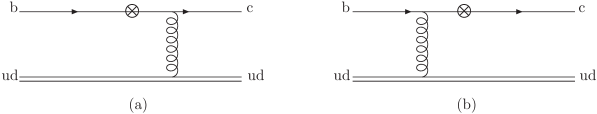
Figure 1: The lowest order diagrams of the hard parts of the transition processes in the quark-diquark picture.

According to the factorization scheme which is depicted in Fig.1, it is straightforward to obtain the analytic expressions of the form factors $F_{1}$, $G_{1}$, $F_{2}$, $G_{2}$, $F_{3}$ and $G_{3}$, by comparing eqs. (4) with (9). In the above derivation, the following transformation has been used.

$$k_{1}=Ap+Bp^{\prime},\qquad k_{2}=Cp+Dp^{\prime}$$ (15)

and the explicit expressions of A,B,C and D are given in the appendix.

Then we can obtain the analytical form of $f_{i}$ and $g_{i}$ (i=1,2,3) making use of the relations between them and $F_{j},G_{j}$(j=1,2,3) listed below

$$f_{1} = F_{1}+\frac{1}{2}(\frac{F_{2}}{M_{\Lambda_{b}}}+\frac{F_{3}}{M_{\Lambda_{c}}})(M_{\Lambda_{b}}+M_{\Lambda_{c}}),\ \ g_{1}=G_{1}-\frac{1}{2}(\frac{G_{2}}{M_{\Lambda_{b}}}+\frac{G_{3}}{M_{\Lambda_{c}}})(M_{\Lambda_{b}}-M_{\Lambda_{c}}),$$

$$f_{2} = -\frac{1}{2}(\frac{F_{2}}{M_{\Lambda_{b}}}+\frac{F_{3}}{M_{\Lambda_{c}}})M_{\Lambda_{b}}^{2},\ \ g_{2}=-\frac{1}{2}(\frac{G_{2}}{M_{\Lambda_{b}}}+\frac{G_{3}}{M_{\Lambda_{c}}})M_{\Lambda_{b}}^{2},$$

$$f_{3} = \frac{1}{2}(\frac{F_{2}}{M_{\Lambda_{b}}}-\frac{F_{3}}{M_{\Lambda_{c}}})M_{\Lambda_{b}}^{2},\ \ g_{3}=\frac{1}{2}(\frac{G_{2}}{M_{\Lambda_{b}}}-\frac{G_{3}}{M_{\Lambda_{c}}})M_{\Lambda_{b}}^{2}.$$ (16)

We do not display the expressions of $f_{3}$ and $g_{3}$ for the reason given above. The form factors are integrations which convolute over three parts Hsiang-nan Li : the hard-part kernel function, the Sudakov factor and the wave functions of the concerned hadrons as

$$f_{i}(g_{i}) = 4\pi C_{F}f_{\Lambda_{b}}f_{\Lambda_{c}}\int^{1}_{0}dx_{1}dx_{2}\int^{\infty}_{0}b_{1}db_{1}b_{2}db_{2}{\int_{0}}^{2\pi}d\theta\ \Phi_{\Lambda_{c}}(x_{2},\mathbf{b}_{2})$$

$$\times kernSgS_{f_{i}(g_{i})}\Phi_{\Lambda_{b}}(x_{1},\mathbf{b}_{1})\exp{[-S(x_{1},x_{2},{\mathbf{b}_{1}},{\mathbf{b}_{2}},r,M_{\Lambda_{b}})]},$$

where the explicit expression of the kernel functions $kernSgS_{f_{i}(g_{i})}$ is given in the appendix for concision of the text. The explicit form of the Sudakov factor appearing in the above equations is given in Ref.Hsiang-nan Li as

$$S(x_{1},x_{2},{\mathbf{b}_{1}},{\mathbf{b}_{2}},r,M_{\Lambda_{b}})$$

$$=s(\omega_{1},(1-x_{l})p^{-})+s(\omega_{2},(1-x_{2})p^{\prime+})+2\int_{\omega_{1}}^{t_{a(b)}}\frac{d\overline{\mu}}{\overline{\mu}}\gamma_{q}(\alpha_{s}(\overline{\mu}))+2\int_{\omega_{2}}^{t_{a(b)}}\frac{d\overline{\mu}}{\overline{\mu}}\gamma_{q}(\alpha_{s}(\overline{\mu})),$$ (18)

where $C_{F}=4/3$ is the color factor.

The wave function $\Phi_{\Lambda_{b}}(x_{1},\mathbf{k}_{1T})$ is Hoi-Lai Yu ; peterson

$$\Phi_{\Lambda_{b}}(x_{1},\mathbf{k}_{1T})=\frac{2N_{b}x_{1}^{6}(1-x_{1})^{3}}{\pi[(1-a_{b}-x_{1})^{2}x_{1}^{2}(1-x_{1})+\varepsilon_{pb}(1-x_{1})^{2}x_{1}^{2}+\mathbf{k}_{1T}^{2}]^{3}},$$ (19)

and

$$\Phi_{\Lambda_{b}}(x_{1},b_{1}) = \int d^{2}\mathbf{k}_{1T}\Phi_{\Lambda_{b}}(x_{1},\mathbf{k}_{1T})e^{i\mathbf{k}_{1T}\cdot\mathbf{b}_{1}}$$ (20)

$$= \frac{N_{b}x_{1}^{6}(1-x_{1})^{3}b_{1}^{2}K_{2}(\sqrt{(1-a_{b}-x_{1})^{2}x_{1}^{2}(1-x_{1})+\varepsilon_{pb}(1-x_{1})^{2}x_{1}^{2}}b_{1})}{2[(1-a_{b}-x_{1})^{2}x_{1}^{2}(1-x_{1})+\varepsilon_{pb}(1-x_{1})^{2}x_{1}^{2}]},$$

where $K_{2}$ is the modified Bessel function of the second kind. If neglecting the transverse momentum $\mathbf{k}_{1T}$, i.e. set $\mathbf{k}_{1T}\sim 0$, the wave function can be simplified as

$$\Phi_{\Lambda_{b}}(x_{1})\simeq\frac{N_{b}x_{1}^{2}(1-x_{1})}{[(1-a_{b}-x_{1})^{2}+\varepsilon_{pb}(1-x_{1})]^{2}}.$$ (21)

The normalization conditions are set as Hoi-Lai Yu

$$\int_{0}^{1}\Phi_{\Lambda_{b}}(x_{1})dx_{1} = 1,$$

$$\int_{0}^{1}\Phi_{\Lambda_{b}}(x_{1})x_{1}dx_{1} = \frac{\bar{\Lambda}}{M_{\Lambda_{b}}},$$

$$\int_{0}^{1}\Phi_{\Lambda_{b}}(x_{1})x_{1}^{2}dx_{1} = (\frac{\bar{\Lambda}^{2}}{M_{\Lambda_{b}}^{2}}+\frac{\lambda_{1}}{3M^{2}_{\Lambda_{b}}}).$$ (22)

The first formula determines the normalization of the parton distribution of the baryon, whereas the second one is related to the effective mass of the light diquark $\bar{\Lambda}\sim M_{\Lambda_{b}}-m_{b}$, and the third formula reflects connection between hadronic matrix element of the kinematic operator $\lambda_{1}=-\frac{1}{2M_{\Lambda_{b}}}\langle\Lambda_{b}\mid\bar{b}_{v}(iD_{\perp})^{2}b_{v}\mid\Lambda_{b}\rangle$ and hadronic distribution amplitude. To satisfy the above three normalization conditions, the parameters would take the following values $\bar{\Lambda}=0.848$ GeV, $\lambda_{1}=-0.76$ GeV², $a_{b}=0.916$, $\varepsilon_{pb}=0.0051$ and $N_{b}=0.0219$, and in the following numerical evaluation, we will use them as inputs.

For the wave function of $\Lambda_{c}$, the expressions are the same as that for $\Lambda_{b}$, while the corresponding parameters are $\bar{\Lambda}=0.8849$ GeV, $\lambda_{1}=-1.87$GeV² , $a_{c}=1.48$, $\varepsilon_{pc}=0.080$ and $N_{c}=12.14$. Thus we can write the differential decay width as

$$\frac{d\Gamma}{d\rho} = \frac{G_{F}^{2}|V_{cb}|^{2}}{24\pi^{3}}M_{\Lambda_{b}}^{5}r^{3}\sqrt{\rho^{2}-1}$$ (23)

$$[\ |f_{1}|^{2}(\rho-1)(3r^{2}-4\rho r+2r+3)+|g_{1}|^{2}(\rho+1)(3r^{2}-4\rho r-2r+3)$$

$$+6\ f_{1}\ f_{2}(r+1)(\rho-1)(r^{2}-2\ r\rho+1)+6\ g_{1}\ g_{2}(r-1)(r^{2}-2\ r\rho+1)$$

$$+|f_{2}|^{2}(\rho-1)(3r^{2}-2\rho r+4r+3)(r^{2}-2\rho r+1)$$

$$+|g_{2}|^{2}(\rho+1)(3r^{2}-2\rho r-4r+3)(r^{2}-2\rho r+1)\ ],$$

with

$$1\leq\rho\leq\rho_{max}=\frac{1}{2}\left(\frac{M_{\Lambda_{b}}}{M_{\Lambda_{c}}}+\frac{M_{\Lambda_{c}}}{M_{\Lambda_{b}}}\right).$$ (24)

III Numerical Results

III.1 The results of PQCD

In the one-heavy-quark-one-light-diquark picture, the $(ud)_{\bar{3}}$ diquark in $\Lambda_{b}$ is considered as a scalar of color anti-triplet. To calculate the form factors in the framework of PQCD, one can adjust the product $f^{S}_{\Lambda_{b}}f^{S}_{\Lambda_{c}}$ to fit the empirical formula $f_{1}(\rho_{max})\sim 1.32/\rho_{max}^{5.18}$ given by the authors of Ref.Li . Then the corresponding parameters are obtained as

$$m_{b}\simeq M_{\Lambda_{b}}=5.624\;{\rm GeV}, m_{c}\simeq M_{\Lambda_{c}}=2.2849\;{\rm GeV}, V_{cb}=0.040,$$

$$f^{S}_{\Lambda_{b}}f^{S}_{\Lambda_{c}}=0.0096\rm{GeV^{2}}, Q^{2}_{0}=3.22\rm{GeV^{2}}, \Lambda_{QCD}=0.2\rm{GeV}.$$ (25)

Using these values, we can continue to numerically estimate the form factors $f_{1}$ and $g_{1}$. Fig.2(a) shows that the form factor $f_{1}$ is exactly equal to $|g_{1}|$ in the heavy quark limit. The form factor $f_{2}$ and $g_{2}$ are much smaller than $f_{1}$ and $|g_{1}|$, thus they can in fact be safely neglected for the present experimental accuracy.

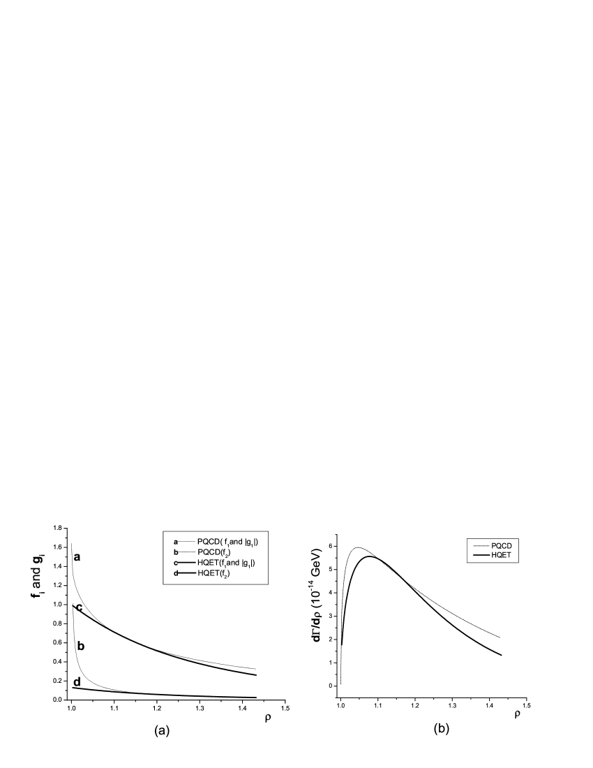
Figure 2: (a) Form factors $f_{2}$, $f_{1}$ and $|g_{1}|$     (b) Differential decay width of $\Lambda_{b}\rightarrow\Lambda_{c}l\nu$

In Fig.2(b), we plot the dependence of the differential width $d\Gamma/d\rho$ on $\rho$. Although both $f_{1}$ and $g_{1}$ have an end-point divergence at $\rho\rightarrow 1$ in PQCD approach, the differential decay rate is finite.

If one extrapolates the PQCD calculation to the region with smaller $\rho$ values, we obtain the form factors $f_{1,2}$ and $g_{1,2}$ in that region where there are obvious end-point singularities at $\rho\to 1$. Redo the computations with the extrapolation (in the original work Li , the authors extend the tangent of the PQCD result at a small $\rho$ value to $\rho=1$, so the end-point singularity is avoided) and obtain $BR(\Lambda_{b}\rightarrow\Lambda_{c}l\nu)$ which is about $1.35\%$ (slightly smaller than the value of 2% guessed by the authors of Ref.Li , because then no data were available. ).

Obviously, the calculation in PQCD depends on the factor $f^{S}_{\Lambda_{b}}f^{S}_{\Lambda_{c}}$, which regularly must be obtained by fitting the data of semileptonic decays, so that the theoretical predictions are less meaningful. Instead, we will use our hybrid scheme where we do not need to obtain the factor $f^{S}_{\Lambda_{b}}f^{S}_{\Lambda_{c}}$ by fitting data, since the connection requirement substitutes the fitting procedure (see below for details).

III.2 The results of HQET

The transition rate was evaluated in terms of HQET by the authors of Ref. xhg . According to the definitions given in eq.(II), we re-calculate $f_{1},\;f_{2},\;g_{1},\;g_{2}$ while dropping out $f_{3}$ and $g_{3}$ and also obtain similar conclusion that $f_{1}$ and $g_{1}$ are the same in amplitude, but opposite in sign, as shown in Fig. 2(a), whereas $f_{2}$ is very small and $g_{2}$ is exactly zero in HQET. The theoretical prediction on the rate of the semi-leptonic decay $\Lambda_{b}\rightarrow\Lambda_{c}+l+\bar{\nu}$ in the HQET is

$$\Gamma(\Lambda_{b}\rightarrow\Lambda_{c}l\bar{\nu}) = 1.54\times 10^{-14}\;{\rm{GeV}},\;\;{\rm without\;contributions\;from}\;f_{2}\;{\rm and}\;g_{2},$$

$$\Gamma(\Lambda_{b}\rightarrow\Lambda_{c}l\bar{\nu}) = 1.56\times 10^{-14}\;{\rm{GeV}},\;\;{\rm with\;contributions\;from}\;f_{2}\;{\rm and}\;g_{2},$$ (26)

and the branching ratio is $2.87\%$.

The transition rate of $\Lambda_{b}\rightarrow\Lambda_{c}l\bar{\nu}$ has recently been measured by the DELPHI Collaboration DELPHI , and the value of $BR(\Lambda_{b}\rightarrow\Lambda_{c}l\nu)$ is $5.0^{+1.1}_{-0.8}(stat)^{+1.6}_{-1.2}(syst)\%$. It is noted that the result calculated in terms of HQET is only consistent with data within two standard deviations.

III.3 The hybrid scheme: Reconciling the two approaches

As widely discussed in literature, in the region with large $q^{2}$ (small $\rho-$values), the result of HQET is reliable, whereas for the region with small $q^{2}$ (larger $\rho-$values) the PQCD is believed to work well. Therefore, to reconcile the two approaches which work in different $\rho$ regions, $1\leq\rho<\rho_{max}$, we apply the HQET for small $\rho$, but use PQCD for larger $\rho$. Our strategy is that we let the form factors $f_{1}$, $g_{1}$ derived in the PQCD approach be equal to the value obtained in terms of HQET at the point $\rho_{cut}$. The numerical results of the form factor $f_{1}=|g_{1}|$ in the hybrid scheme are shown in Fig.3 for three different $\rho_{cut}-$values: 1.05, 1.10 and 1.15, respectively. It is noted that for $\rho_{cut}=1.1$ and 1.15, the left- and right-derivatives are very close and the connection is smooth, whereas, as $\rho_{cut}$ is chosen as 1.05, a difference between the derivatives at the two sides of $\rho_{cut}=1.05$ obviously manifests. We then adopt a proper numerical program to smoothen the curve, namely let the derivatives of the two sides meet each other for any $\rho-$value near the cut point. Fig.3 shows that such treatment in fact does not change the general form of the curve, but makes it sufficiently smooth for all $\rho$ values including the selected cut point $\rho_{cut}$.

Another advantage of adopting such a “hybrid” scheme is that there does not exist end-point singularity for the form factors at $\rho=1$. Since at the turning point, we let the form factors derived in terms of PQCD be connected with that obtained in HQET, the product $f_{\Lambda_{b}}f_{\Lambda_{c}}$ is automatically determined by the connection. With the value, we calculate the form factors within the range of small $q^{2}$ in PQCD. In this hybrid scheme, one does not need to invoke the data on the semi-leptonic decay to fix the parameter $f_{\Lambda_{b}}f_{\Lambda_{c}}$ at all.

By our numerical results obtained in the hybrid scheme, the form factors $f_{1}$ (or $g_{1}$) can be parameterized in a satisfactory expression, here we only present the expression for $\rho_{cut}=1.10$ as

$$f_{1}(\rho)=1-3.61(\rho-1)+7.24(\rho-1)^{2}-5.83(\rho-1)^{3},$$ (27)

and similar parameterized form factors were discussed in ref.cheng .

The expression can be described by only one “Isger-Wise function” for the transition $\Lambda_{b}\rightarrow\Lambda+l\bar{l}$ at the heavy quark limit, and it is done by the DELPHI collaboration based on their data on $\Lambda_{b}\rightarrow\Lambda_{c}l\bar{\nu}$. It is parameterized as DELPHI

$$\xi(\omega)=1-\hat{\rho}^{2}(\omega-1)+O((\omega-1)^{2}),$$ (28)

where $\hat{\rho}^{2}=2.03\pm 0.46(stat)^{+0.72}_{-1.00}(syst)$.

Obviously, this expression is only valid to the leading order, i.e. linearly proportional to $\omega-1$ where $\omega$ exactly corresponds to the parameter $\rho$ which is commonly adopted in the PQCD language. By contrast, our result includes higher power terms because the $1/M$ corrections are automatically taken into account in our work. It is noted that the coefficient of the linear term in our numerical result is reasonably consistent with the $\hat{\rho}^{2}$ obtained by fitting data.

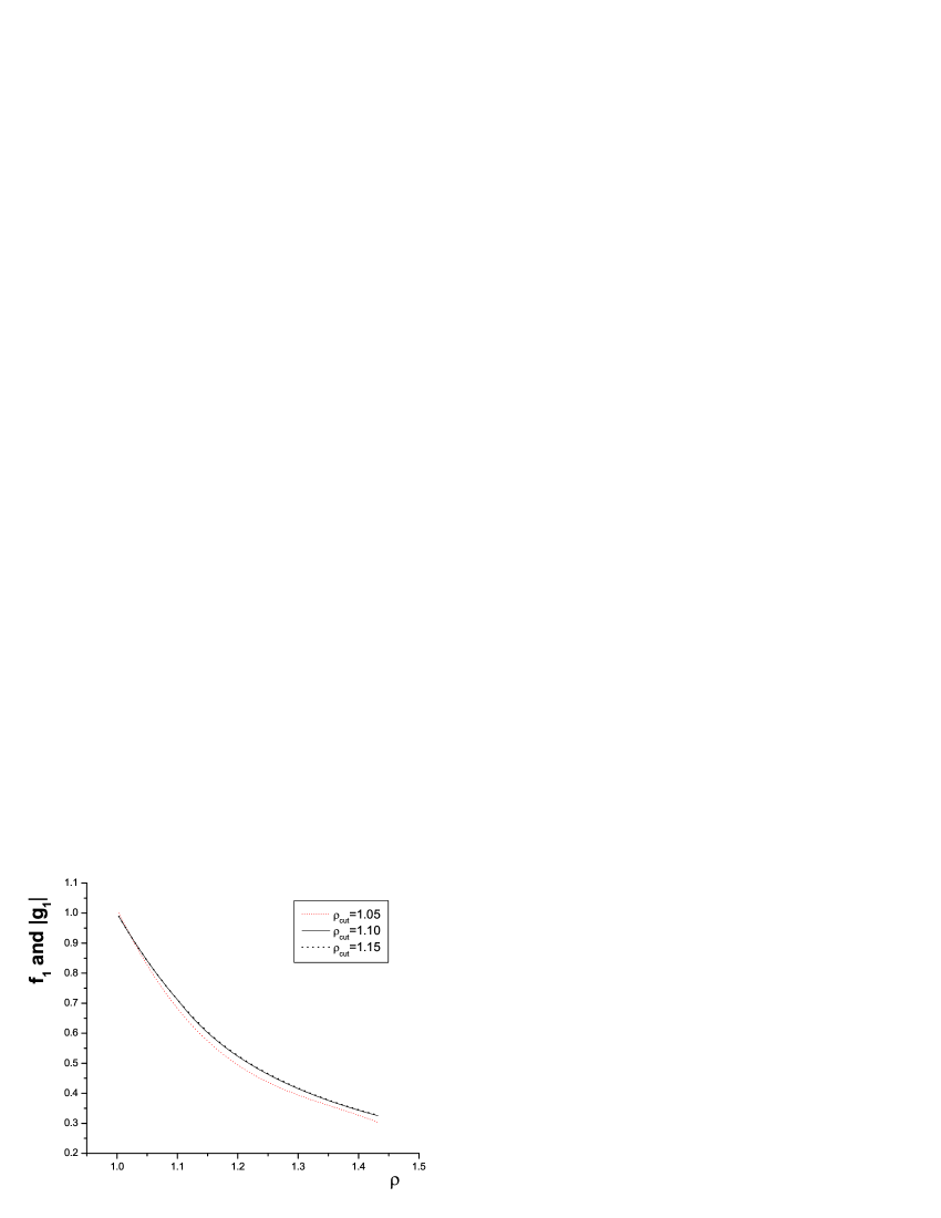
Figure 3: Form factors $f_{1}=|g_{1}|$ in the hybrid scheme

To obtain the total decay width, we integrate over the whole range $\rho$ from 1 to $\rho_{max}$, the integrand is the parameterized form factor in eq.(27). We obtain

$$\Gamma(\Lambda_{b}\rightarrow\Lambda_{c}l\nu)=1.65\times 10^{-14}{\rm{GeV}},\;\;BR=3.08\%\;\;\;\;\;{\rm with}\;\rho_{cut}=1.10,\;\;f_{\Lambda_{b}}f_{\Lambda_{c}}=0.0149\;{\rm{GeV}^{2}}.$$ (29)

For a comparison, we present the results corresponding to other two $\rho_{cut}$ values where the smoothing treatment is employed, and they are

$$\Gamma(\Lambda_{b}\rightarrow\Lambda_{c}l\nu) = 1.54\times 10^{-14}\;{\rm{GeV}},\;\;BR=2.87\%\;\;\;\;\;\rho_{cut}=1.05,\;\;f_{\Lambda_{b}}f_{\Lambda_{c}}=0.0142\;\rm{{GeV}^{2}};$$

$$\Gamma(\Lambda_{b}\rightarrow\Lambda_{c}l\nu) = 1.67\times 10^{-14}\;{\rm{GeV}},\;\;BR=3.12\%\;\;\;\;\;\rho_{cut}=1.15;\;\;f_{\Lambda_{b}}f_{\Lambda_{c}}=0.0150\;\rm{{GeV}^{2}}.$$ (30)

One can notice that the factor $f_{\Lambda_{b}}f_{\Lambda_{c}}$ does not change much as $\rho_{cut}$ varies and they are about 1.5 times larger than the value obtained in pure PQCD (eq.(III.1)). When the turning point is chosen at $\rho_{cut}=1.05$, the branching ratio calculated in the hybrid scheme is very close to the result obtained in pure HQET, while for $\rho_{cut}=1.10$ and $\rho_{cut}=1.15$, the resultant branching ratio is slightly larger than that obtained in pure HQET, but more coincides with the data.

Figure 4: The $G_{1}/F_{1}$ ratio obtained in our hybrid scheme

In our scenario, the HQET is applied for smaller $\rho$, and the values of the form factors at $\rho_{cut}$ are fixed by the theory. The values can also determine $f_{\Lambda_{b}}f_{\Lambda_{c}}$ which will be used for the PQCD calculations for larger $\rho$. The HQET is an ideal theoretical framework, but there is an unknown function which is fully governed by the non-perturbative QCD effects, that is the famous Isgur-Wise function. The function can be either obtained by fitting data, or evaluated by concrete models. Various models would result in different slopes. The authors of ref. xhg used the Drell-Yan type overlap integrals to obtain the slope which is what we employed to get the parametrization eq.(27) and the slope is $-3.6$. Instead, the authors of Liu1 evaluated the slope in the Isgur-Wise function by means of the QCD sum rules. According to their result, we re-parameterize the form factor $f_{1}(\rho)$ and have

$$f_{1}(\rho)=1.01-1.57(\rho-1)-2.59(\rho-1)^{2}+6.99(\rho-1)^{3}.$$ (31)

Correspondingly, we obtain

$$\Gamma(\Lambda_{b}\rightarrow\Lambda_{c}l\nu)=2.38\times 10^{-14}{\rm{GeV}},\;\;BR=4.45\%\;\;\;\;\;{\rm with}\;\rho_{cut}=1.10,\;\;f_{\Lambda_{b}}f_{\Lambda_{c}}=0.0213\;{\rm{GeV}^{2}}.$$ (32)

The fitted slope by the DELPHI collaboration is $\hat{\rho}^{2}=2.03\pm 0.46(stat)^{+0.72}_{-1.00}(syst)$ DELPHI , which is between the two theoretical evaluated values. In these references, only linear term remained, due to uncertainties in the approximations the deviations are understandable. Therefore, one can note that there is a model-dependence which mainly manifests in the slope of the Isgur-Wise function. Even though they deviate from each other at the linear term, the high power terms would compensate the deviation slightly and the predicted values on the branching ratio in two approaches eqs.(27,31) are qualitatively consistent with data. There indeed is a byproduct which brings in an advantage that more accurate measurements can help to make judgement on validity of the models by which the Isgur-Wise functions are evaluated.

To make more sense, we purposely present the ratio $G_{1}/F_{1}$ obtained in the hybrid scheme in Fig. 4, it is noted that the ratio is qualitatively consistent with that given in ref. Kroll which was shown on the left part of Fig. 3 of their paper Kroll .

The authors of ref. Kroll extended $\rho$ into the un-physical region ($\rho>\rho_{max}$ for $\Lambda_{b}\rightarrow\Lambda_{c}l\bar{\nu}$), while we only keep it within the physical region. It is noted that in the physical region, numerically our result is very close to that obtained in ref. Kroll . But if one extends the curve to larger $\rho$, he will notice that our curve is convex, but theirs is concave, namely the coefficient of the quadratic term has an opposite sign, but the difference is too tiny to be observed or bring up substantial difference for the evaluation of the decay width.

IV discussion and conclusion

In this work, we investigate the semi-leptonic decay $\Lambda_{b}\to\Lambda_{c}+l+\bar{\nu}_{l}$ in the so called “hybrid scheme” and the diquark picture for heavy baryons $\Lambda_{b}$ and $\Lambda_{c}$. The hybrid scheme means that for the range of smaller $q^{2}$ (larger $\rho-$value) we use the PQCD approach, whereas the HQET for larger $q^{2}$ (near $\rho=1$), to calculate the form factors. We find that the form factors $f_{2}$ and $g_{2}$ can be safely neglected as suggested in the literature. Besides, we do not need to determine the phenomenological parameters $f_{\Lambda_{b}}$ and $f_{\Lambda_{c}}$ by fitting data in the hybrid scheme as one did with the pure PQCD approach. Our result is generally consistent with the newly measured branching ratio $\Lambda_{b}\to\Lambda_{c}+l+\bar{\nu}_{l}$ within two standard deviations and the end-point singularities existing in the PQCD approach are completely avoided. In fact, the final result somehow depends on the slope in the Isgur-Wise function of the HQET, which is obtained by model-dependent theoretical calculations. Therefore, we may only trust the obtained value to this accuracy, the further experimental data and development in theoretical framework will help to improve the accuracy of the theoretical predictions.

The quark-diquark picture seems to work well for dealing with the semi-leptonic decays of $\Lambda_{b}$, and we may expect that the quark-diquark picture indeed reflects the physical reality and is applicable to the processes where baryons are involved, at least for the heavy baryons Guo . This picture will be further tested in the non-leptonic decays of heavy baryons. We will employ the diquark picture and PQCD to further study the non-leptonic decay modes in our future work.

Appendix A Explicit expressions of hard kernel

$$kernSgS_{f_{1}} = \Big{\{}\Big{[}(BC-AD)(1+r)-(C^{2}-A(2-C+Dr)+(B+D)r(Dr-2\rho)+$$

$$C(Br+2Br\rho+2Dr\rho-2))\Big{]}hha+\Big{[}(BC-AD)r\ (1+r)-\ (A^{2}+A$$

$$(C-r(D+2\rho-2B\rho))+r(B^{2}r-2(Dr+C\rho)-B(C+(-2+D)r$$

$$+2C\rho)))\Big{]}hhb\Big{\}}{M^{2}_{\Lambda_{b}}}F_{S}(\eta),$$

$$kernSgS_{g_{1}} = \Big{\{}\Big{[}(BC-AD)(r-1)+(C^{2}+A(-2+C+Dr)+(B+D)r(Dr-2\rho)-$$

$$C(rB-2Dr\rho-2rB\rho+2))\Big{]}hha+\Big{[}(BC-AD)\ r(1-r)+(A^{2}+A$$

$$(C+r(D-2\rho+2B\rho))+r(B^{2}r-2(Dr+C\rho)+B\ ((-2+D)r-C$$

$$+2C\rho)))\Big{]}hhb\Big{\}}\ {M^{2}_{\Lambda_{b}}}F_{S}(\eta),$$

$$kernSgS_{f_{2}} = (AD-BC)\ (hha+r\ hhb)\ M^{2}_{\Lambda_{b}}F_{S}(\eta),$$

$$kernSgS_{g_{2}} = (AD-BC)\ (hha-r\ hhb)\ M^{2}_{\Lambda_{b}}F_{S}(\eta),$$

where

$$\eta\equiv M_{\Lambda_{b}}M_{\Lambda_{c}}x_{1}x_{2}\xi_{1}.$$ (34)

The explicit expressions of A, B, C and D

$$A=\frac{x_{1}\ \xi_{1}}{\xi_{1}-\xi_{2}},\qquad\ B=-\frac{x_{1}\ M_{\Lambda_{b}}}{M_{\Lambda_{c}}(\xi_{1}-\xi_{2})},$$

$$C=-\frac{x_{2}\ M_{\Lambda_{c}}}{M_{\Lambda_{b}}(\xi_{2}-\xi_{1})},\qquad\ D=\frac{x_{2}\ \beta_{1}}{\xi_{1}-\xi_{2}},$$ (35)

with

$$\xi_{1}=\rho+\sqrt{\rho^{2}-1},\qquad\xi_{2}=\rho-\sqrt{\rho^{2}-1}.\\$$

The explicit expressions of $hha$, $hhb$ are

$$hha = \alpha_{s}(t_{a})K_{0}(\sqrt{x_{1}x_{2}\xi_{1}M_{\Lambda_{b}}M_{\Lambda_{c}}}b_{1})K_{0}(\sqrt{x_{2}\xi_{1}M_{\Lambda_{b}}M_{\Lambda_{c}}}|\textbf{b}_{1}+\textbf{b}_{2}|),\,\,\,\,\,\,$$

$$hhb = \alpha_{s}(t_{b})K_{0}(\sqrt{x_{1}x_{2}\xi_{1}M_{\Lambda_{b}}M_{\Lambda_{c}}}b_{2})K_{0}(\sqrt{x_{1}\xi_{1}M_{\Lambda_{b}}M_{\Lambda_{c}}}|\textbf{b}_{1}+\textbf{b}_{2}|),\,\,\,\,\,\,$$ (36)

with

$$t_{a}=max(\sqrt{x_{2}\xi_{1}M_{\Lambda_{b}}M_{\Lambda_{c}}},1/|\textbf{b}_{1}+\textbf{b}_{2}|,1/b_{1},1/b_{2}),$$

$$t_{b}=max(\sqrt{x_{1}\xi_{1}M_{\Lambda_{b}}M_{\Lambda_{c}}},1/|\textbf{b}_{1}+\textbf{b}_{2}|,1/b_{1},1/b_{2}).$$

References

• (1) H. Li and G. Sterman, Nucl. Phys. B 381,129 (1992); G. Korchemsky and G. Sterman, Phys. Lett. B 340, 96 (1994); J. Botts and G. Sterman, Nucl. Phys. B 325, 62 (1989).
• (2) Y. Keum, H. Li, A.I. Sanda, Phys. Lett. B 504, 6 (2001); Phys. Rev. D 63, 054008 (2001); C. LΓΌ, K. Ukai, M. Yang, Phys. Rev. D 63, 074009 (2001).
• (3) H. Shih, S. Lee and H. Li, Phys. Rev. D 61, 114002 (2000).
• (4) N. Isgur and M. Wise, Phys. Lett. B232, 113 (1989); N. Isgur and M. Wise, Nucl.Phys. B 348, 276 (1991) ; H. Georgi, ibid B348, 293 (1991).
• (5) J. Abdallah et al, DELPHI Collaboration, Phys. Lett. B585, 63 (2004) .
• (6) M. Huang , H. Jin , J. K$\rm{\ddot{o}}$rner and C. Liu Phys. Lett. B629, 27 (2005).
• (7) Y. Dai, C. Huang, M. Huang and C. Liu, Phys. Lett. B 387, 379 (1996); Y. Dai, C. Huang, C. Liu and C. D. LΓΌ, ibid B 371, 99 (1996); C. Liu Phys. Rev. D 57, 1991 (1998) ; J. Lee, C. Liu and H. Song, ibid D 58, 014013 (1998).
• (8) X. H. Guo, P. Kroll, Z. Phys. C 59, 567 (1993);
• (9) F. Wilczek, hep-ph/0409168.
• (10) A. Flak and M. Neubert, Phys. Rev. D 47, 2982 (1993) ; B. Holdom, M. Sutherland and J. Mureika, ibid D49, 2359 (1994).
• (11) J. K$\rm{\ddot{o}}$rner and P. Kroll, Z. Phys. C 57, 383 (1993).
• (12) H. Li, Phys. Rev. D 52, 3958 (1995).
• (13) H. Li and H. Yu, Phys.Rev.D 53, 4970 (1996) .
• (14) H. Shih, S. Lee and H. Li, Phys.Rev. D 59, 094014 (1999); C.H. Chou, H. Shih, S. Lee and H. Li, Phys. Rev. D 65, 074030 (2002).
• (15) R. Jakob, P. Kroll, M. Schuermann and W. Schweiger, Z. Phys. A 347, 109 (1993).
• (16) C. Peterson, D. Schlatter, I. Schmitt and P. Zerwas, Phys. Rev. D 27, 105 (1983) .
• (17) H. Cheng, C. Cheung and C. Hwang , Phys. Rev. D 69, 074025 (2004) .
• (18) X. Guo and T. Muta, Phys. Rev. D 54, 4629 (1996) ; X. Guo, A. Thomas and A. Williams, ibid D 59, 116007 (1999) .