Abstract

In this work we show that the physics reach of a long-baseline (LBL) neutrino oscillation experiment based on a superbeam and a megaton water Cherenkov detector can be significantly increased if the LBL data are combined with data from atmospheric neutrinos (ATM) provided by the same detector. ATM data are sensitive to the octant of $\theta_{23}$ and to the type of the neutrino mass hierarchy, mainly through three-flavor effects in $e$-like events. This allows to resolve the so-called $\theta_{23}$- and sign($\Delta m_{31}^{2}$)-parameter degeneracies in LBL data. As a consequence it becomes possible to distinguish the normal from the inverted neutrino mass ordering at $2\sigma$ CL from a combined LBL+ATM analysis if $\sin^{2}2\theta_{13}\gtrsim 0.02$. The potential to identify the true values of $\sin^{2}2\theta_{13}$ and the CP-phase $\delta_{\mathrm{CP}}$ is significantly increased through the lifting of the degeneracies. These claims are supported by a detailed simulation of the T2K (phase II) LBL experiment combined with a full three-flavor analysis of ATM data in the HyperKamiokande detector.

1 Introduction

Thanks to the out-standing developments in recent neutrino physics a rather clear picture of neutrino oscillation parameters is emerging. We know that there are two large angles in the lepton mixing matrix, $\theta_{12}$ and $\theta_{23}$, and one small angle $\theta_{13}$, and the mass-squared differences $\Delta m_{21}^{2}$ and $|\Delta m_{31}^{2}|$ are well determined by the global data from solar [1] atmospheric [2], reactor [3], and accelerator [4] neutrino experiments. A recent global analysis of world neutrino oscillation data can be found e.g. in Ref. [5]. Despite these enormous achievements there are still important open questions related to neutrino physics, which have to be addressed by future neutrino oscillation experiments:

1. What is the value of the mixing angle $\theta_{13}$?

2. What is the value of the complex phase $\delta_{\mathrm{CP}}$ in the mixing matrix?

3. Is the neutrino mass ordering normal ($m_{1}<m_{2}<m_{3}$) or inverted ($m_{3}<m_{1}<m_{2}$), i.e., what is the sign of $\Delta m_{31}^{2}$?

In contrast to the “discovery phase”, which was dominated by natural neutrino sources such as the sun or the atmosphere, the subsequent generation of oscillation experiments will be mainly based on man-made neutrinos, where the neutrino source is well under control. Among the future projects are conventional beam experiments [6], new reactor experiments [7], superbeam experiments [8, 9], and eventually experiments based on a neutrino factory or a beta-beam [10].

A characteristic feature in the analysis of future long-baseline (LBL) experiments is the presence of so-called parameter degeneracies, see e.g., Refs. [11, 12, 13, 14, 15, 16, 17]. Due to the inherent three-flavor structure of the oscillation probabilities, for a given experiment in general several disconnected regions in the multi-dimensional space of oscillation parameters will be present. Traditionally these degeneracies are referred to in the following way:

• The intrinsic or ($\delta_{\mathrm{CP}},\theta_{13}$)-degeneracy [18, 19]: For a measurement based on the $\nu_{\mu}\to\nu_{e}$ oscillation probability for neutrinos and anti-neutrinos two disconnected solutions appear in the ($\delta_{\mathrm{CP}},\theta_{13}$) plane.

• The hierarchy or sign($\Delta m_{31}^{2}$)-degeneracy [20]: The two solutions corresponding to the two signs of $\Delta m_{31}^{2}$ appear in general at different values of $\delta_{\mathrm{CP}}$ and $\theta_{13}$.

• The octant or $\theta_{23}$-degeneracy [21]: Since LBL experiments are sensitive mainly to $\sin^{2}2\theta_{23}$ it is difficult to distinguish the two octants $\theta_{23}<\pi/4$ and $\theta_{23}>\pi/4$. Again, the solutions corresponding to $\theta_{23}$ and $\pi/2-\theta_{23}$ appear in general at different values of $\delta_{\mathrm{CP}}$ and $\theta_{13}$.

This leads to an eight-fold ambiguity in the determination of $\theta_{13}$ and $\delta_{\mathrm{CP}}$ [11], and hence degeneracies provide a serious limitation in the ability to answer the questions 1 and 2 above. Moreover, the fact that one speaks of a “sign($\Delta m_{31}^{2}$)-degeneracy” illustrates that answering question 3 is difficult: determining the neutrino mass ordering is equivalent to resolving the sign($\Delta m_{31}^{2}$)-degeneracy. Several methods to resolve these degeneracies have been proposed, among them the combination of experiments at various baselines and/or $(L/E)$-values [22, 23, 20, 11, 24, 25], the use of spectral information [12, 26], the combination of $\nu_{e}\to\nu_{\mu}$ and $\nu_{e}\to\nu_{\tau}$ oscillation channels [27], and the combination of LBL and reactor experiments [28, 29, 30, 31, 32].

In the present work we discuss a new possibility to resolve the LBL parameter degeneracies, based on the data from atmospheric neutrinos. It is known that atmospheric neutrinos are in principle sensitive to $\theta_{13}$ and the neutrino mass hierarchy due to earth matter effects [33] in the $e$-like events [34, 35, 36, 37, 38, 39, 40]. These effects are most pronounced in the multi-GeV energy range and for large zenith angles, corresponding to neutrino trajectories crossing the earth mantle or the mantle and the core. In addition effects from the solar parameters $\theta_{12}$ and $\Delta m_{21}^{2}$ on $e$-like events in the sub-GeV energy range provide sensitivity to the octant of $\theta_{23}$ [41, 42, 43], and in principle even on $\delta_{\mathrm{CP}}$ [44]. For a recent discussion of sub-leading effects in atmospheric neutrino oscillations see Ref. [45]. It turns out, however, that atmospheric (ATM) data on its own can never compete with LBL in many respects, such as the determination of $\theta_{13},\delta_{\mathrm{CP}},|\Delta m_{31}^{2}|$, or $\sin^{2}2\theta_{23}$. One reason is that they are limited by systematical uncertainties, e.g. from the neutrino fluxes. However, as we will show in the following, due to the effects mentioned above ATM data can break the sign($\Delta m_{31}^{2}$)- and $\theta_{23}$-degeneracies in LBL data, and hence the combined analysis of LBL and ATM leads to significant synergies.

An important part of the future neutrino program are gigantic water Cherenkov detectors at the megaton scale. Apart from serving as detector for LBL experiments such a facility will provide unprecedented opportunities for proton decay, solar and atmospheric neutrino experiments, as well as for the detection of supernova and other astrophysical neutrinos. The projects under discussion are UNO [46] in the US, a megaton detector in the Frejus laboratory [47] in Europe, and the HyperKamiokande project [9, 40] in Japan. If a LBL experiment with such a detector will be built atmospheric neutrino data come for free. Therefore, our method provides a very efficient possibility to resolve the parameter degeneracies from LBL data, in contrast to the previously discussed methods, which in general are based on the combination of two or more expensive experiments.

In the following we will illustrate how the LBL+ATM combination works by considering the phase II of the T2K experiment (T2K-II) [9], assuming a 4 MW superbeam produced at the J-PARC accelerator, and the 1 Mt HyperKamiokande (HK) detector serving as the far detector for the LBL experiment as well as providing the high statistics atmospheric neutrino data. Let us note that similar results are expected also for the other megaton detector proposals. Furthermore, if huge magnetized iron detectors are available one expects similar synergies between LBL and ATM data. For these type of detectors the ability to distinguish between neutrinos and anti-neutrinos will increase the potential of ATM data even further [48]. In the present work we stick to the HK water Cherenkov detector, the potential of magnetized detectors will be considered elsewhere.

The outline of the paper is as follows. In Section 2 we give some technical details of our simulation of the T2K-II experiment (Section 2.1) and of the atmospheric neutrino analysis (Section 2.2), and we describe the statistical methods used in the following (Section 2.3). In Section 3 we illustrate the LBL/ATM complementarity by discussing the effects of parameter degeneracies for the LBL data (Section 3.1), whereas in Sections 3.2 and 3.3 we consider the effects in ATM data which allow to resolve the octant and the sign($\Delta m_{31}^{2}$) degeneracies, respectively. In Section 4 we investigate in detail the ability to exclude degenerate solutions with LBL+ATM data by performing a systematic scan of the parameter space of $\theta_{13}$, $\theta_{23}$ and $\delta_{\mathrm{CP}}$. In Section 5 we discuss the potential to identify the neutrino mass ordering, for the special case $\theta_{23}=\pi/4$ (Section 5.1) as well as for the general case (Section 5.2). In Section 6 we show how the sensitivity to $\theta_{13}$ is improved by resolving the $\theta_{23}$-degeneracy by ATM data, and we summarize our results in Section 7.

2 Description of the experiments and statistical analysis

2.1 The T2K-II long-baseline experiment

In the following the label “LBL” refers to the phase II of the T2K experiment (T2K-II) [9]. We are assuming a high luminosity superbeam with mean neutrino energy of 0.76 GeV, produced with a target power of 4 MW at the J-PARC accelerator. The neutrinos are detected at a 1 Mt water Cherenkov detector, HyperKamiokande (HK), at a baseline of 295 km and an off-axis angle of $2^{\circ}$. We consider 2 years running time with a neutrino beam, and 6 years with anti-neutrinos, such that comparable event numbers are obtained for neutrinos and anti-neutrinos.

Our simulation of the T2K-II experiment is performed by using the GLoBES software package [49]. We take into account realistic neutrino fluxes, detection cross sections, energy resolution, and efficiencies [9]. This experimental information is folded with the three-flavor oscillation probability, fully taking into account the earth matter effect. We consider all available information, from $\nu_{\mu}\to\nu_{e}$ appearance, as well as $\nu_{\mu}$ disappearance channels. The signal events are given by $\nu_{e}$ and $\nu_{\mu}$ charged current (CC) interactions, respectively. We divide the signal into the total event rate, where the full CC cross section is used, and into the energy spectrum with free normalization, where only events from quasi-elastic scattering are used, since non-quasi-elastic events do not allow to reconstruct the neutrino energy. Various backgrounds such as a $\nu_{e}$ contamination of the beam, $\nu_{\mu}$ neutral current events, and misidentification of muon neutrinos as electron neutrinos are taken into account, using information given in Ref. [9]. We list the numbers of signal and background events expected in T2K-II for typical oscillation parameters in Table 1. More details of our T2K-II analysis can be found in Ref. [13].

The T2K-II LBL experiment			The HK ATM experiment (9 Mt yrs)
	$\nu$ (2 Mt yrs)	$\bar{\nu}$ (6 Mt yrs)		$\nu$	$\bar{\nu}$
$\nu_{\mu}\to\nu_{e}$ signal	21 300	16 000	$e$-like sub-GeV	239 000	58 000
$\nu_{\mu}\to\nu_{e}$ background	2 140	3 260	$e$-like multi-GeV	52 700	18 100
$\nu_{\mu}\to\nu_{\mu}$ signal	73 200	75 600	$\mu$-like sub-GeV	232 000	66 200
$\nu_{\mu}\to\nu_{\mu}$ background	340	320	$\mu$-like multi-GeV	108 000	49 100
			upward going $\mu$	127 000	65 400

Table 1: Number of events in the LBL and ATM experiments considered in our work for the oscillation parameters $\sin^{2}2\theta_{13}=0.05$, $\sin^{2}\theta_{23}=0.5$, $\sin^{2}\theta_{12}=0.3$, $\delta_{\mathrm{CP}}=0$, $\Delta m_{21}^{2}=8.1\times 10^{-5}$ eV², and $\Delta m_{31}^{2}=2.2\times 10^{-3}$ eV².

2.2 The HK atmospheric neutrino experiment

To simulate atmospheric neutrino data in the HK detector we follow closely Ref. [43]. A crucial element of the analysis is to take into account the full three-flavor oscillation probability, including earth matter effects, as well as oscillations induced by the “solar” mass splitting $\Delta m_{21}^{2}$ (for other three-flavor analyses see Refs. [50, 51, 52, 53]). In our analysis we consider charged current data, divided into sub-GeV and multi-GeV $e$-like and $\mu$-like contained event samples (each grouped into 10 bins in zenith angle), as well as stopping (5 angular bins) and through-going (10 angular bins) up-going muon events.

Details of our statistical analysis can be found in the Appendix of Ref. [54]. Together with the statistical errors, we consider theoretical as well as systematical uncertainties, where theoretical uncertainties are uncertainties in the original atmospheric neutrino fluxes and in the cross-sections. We are using the atmospheric neutrino fluxes from Ref. [55], and flux uncertainties include total normalization errors (20%) allowing for an independent fluctuation of neutrino and anti-neutrino fluxes (5%) as well as $\nu_{\mu}$ and $\nu_{e}$ fluxes (5%), spectral uncertainty of the fluxes (“tilt” factor), and an uncertainty on the zenith angle dependence which induces an error in the up/down asymmetry of events (5%). We also include independent normalization errors for the different contributions to the interaction cross section: quasi-elastic scattering (15%), single pion production (15%), and deep inelastic scattering (15% for contained events and 10% for upward-going muons). Moreover, we include as systematical errors experimental uncertainties associated with the simulation of the hadronic interactions, the particle identification procedure, the ring-counting procedure, the fiducial volume determination, the energy calibration, the relative normalization between partially-contained and fully-contained events, the track reconstruction of up-going muons, the detection efficiency of up-going muons, and the stopping/through-going separation.

The current atmospheric neutrino data sample from SuperKamiokande (SK-I) consists of 1489 days of data (contained events) with a detector mass of 22.5 kt, which gives roughly $90\,\mathrm{kt\,yrs}$ of data. In this work we are considering a data taking period for the LBL experiment of 8 years. We assume that the 1 Mt HK detector will be finished one year before the T2K-II beam, and hence $9\,\mathrm{Mt\,yrs}$ of atmospheric neutrino data will be available. For the atmospheric data sample used in our analysis, which we will denote in the following by the label “ATM”, we scale the present SK-I sample (1489 days contained events, 1657 days of stopping, and 1678 days of through-going muons) by a factor 100. Event numbers for various ATM data samples for typical oscillation parameters are given in Table 1.

2.3 Details of the statistical analysis

In order to investigate the potential of the experiments described in the previous sub-sections we adopt the standard method for analyzing future experiments. First, artificial “data” is simulated by calculating event numbers for LBL and ATM for some “true values” $\boldsymbol{\theta}^{\mathrm{true}}$ for the oscillation parameters $\boldsymbol{\theta}=(\theta_{13},\theta_{12},\theta_{23},\delta_{\mathrm{CP}},\Delta m_{21}^{2},\Delta m_{31}^{2})$. Then a $\chi^{2}$-analysis of these “data” is performed to extract allowed regions for the oscillation parameters. It is important to note that in general the results will depend on the values adopted for $\boldsymbol{\theta}^{\mathrm{true}}$. For all calculations we will use for $\theta_{12}^{\mathrm{true}},(\Delta m_{21}^{2})^{\mathrm{true}}$ and $(\Delta m_{31}^{2})^{\mathrm{true}}$ the best fit values obtained in Ref. [5],

$$\sin^{2}\theta_{12}=0.3\,,\quad\Delta m_{21}^{2}=8.1\times 10^{-5}\,\mathrm{eV}^{2}\,,\quad|\Delta m_{31}^{2}|=2.2\times 10^{-3}\,\mathrm{eV}^{2}\,.$$ (1)

We do not expect any significant changes of our results if these parameters are varied within the present allowed ranges [5]. However, we adopt various values for $\theta_{13}^{\mathrm{true}},\theta_{23}^{\mathrm{true}}$, $\delta_{\mathrm{CP}}^{\mathrm{true}}$, and sign($\Delta m_{31}^{2}$), and show our results as a function of these parameters. Furthermore, since neither LBL nor ATM data allow an accurate determination of $\theta_{12}$ and $\Delta m_{21}^{2}$ we assume that these two parameters are known with an uncertainty of 10% from solar and reactor neutrino experiments.

If one is interested in the allowed range for a certain parameter $\xi\in\boldsymbol{\theta}$ for a given choice of $\boldsymbol{\theta}^{\mathrm{true}}$, the function $\chi^{2}(\boldsymbol{\theta}^{\mathrm{true}};\boldsymbol{\theta})$ has to be minimized with respect to all other parameters $\boldsymbol{\theta}$ except $\xi$ to take into account the correlations and degeneracies between parameters. This minimization is performed by using the GLoBES software package [49], which has been generalized in order to include the atmospheric neutrino code. Let us stress that for both data samples, LBL as well as ATM, a full three-flavor analysis including matter effects is performed. The only approximation is to neglect the (very weak) dependence on $\theta_{12}$. Since LBL depends in leading order only on the product $\sin 2\theta_{12}\Delta m_{21}^{2}$ fixing $\theta_{12}$ does not introduce any error, as long as the dependence on $\Delta m_{21}^{2}$ is properly taken into account, and for ATM varying $\theta_{12}$ in the allowed range is expected to have a very small impact. Apart from this simplification the full parameter dependence of both data sets has been taken into account. However, we assume that LBL and ATM data are statistically independent. This might not be completely correct since both data sets are based on the same detector, and hence, uncertainties related to the detection process can introduce correlations between LBL and ATM data. Although such effects will have to be included eventually in the analysis of real data, we expect that such correlations introduce only very minor corrections to our present results.

3 Complementarity between LBL and ATM data

3.1 Parameter degeneracies and the T2K-II experiment

In this section we discuss the problem of parameter degeneracies for the T2K-II experiment. First we note that for this particular experiment the $(\delta_{\mathrm{CP}},\theta_{13})$-degeneracy does not occur. It is known that for experiments operating at the oscillation maximum of $\Delta m_{31}^{2}$ the second solution in the $(\delta_{\mathrm{CP}},\theta_{13})$ plane can be disfavored efficiently [11, 13]. Moreover, spectral information is important, since $\delta_{\mathrm{CP}}$-dependent and $\delta_{\mathrm{CP}}$-independent terms in the oscillation probability show a different energy dependence (compare Eq. (3.1) later in this section). Thus it is difficult to leave the spectrum unchanged when $\delta_{\mathrm{CP}}$ is varied, and the $(\delta_{\mathrm{CP}},\theta_{13})$-degenerate solution, which implies a different value of $\delta_{\mathrm{CP}}$, is disfavored. An illustration of the relevance of spectral information for the $(\delta_{\mathrm{CP}},\theta_{13})$-degeneracy in the T2K-II experiment can be found in Figure 5 of Ref. [13].

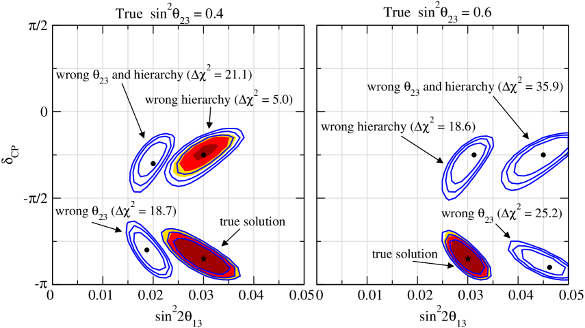
Therefore, in the case of T2K-II we are confronted only with the sign($\Delta m_{31}^{2}$)- and $\theta_{23}$-degeneracies. Apart from the incapacity to determine the neutrino mass ordering and the octant of $\theta_{23}$ this leads to a four-fold ambiguity in the determination of $\theta_{13}$ and $\delta_{\mathrm{CP}}$. The impact of the degeneracies can be appreciated in Figure 1, where the solid curves show the allowed regions from LBL data in the $(\sin^{2}2\theta_{13},\delta_{\mathrm{CP}})$ plane for an example-point with the true values $\sin^{2}2\theta_{13}=0.03$, $\delta_{\mathrm{CP}}=-0.85\pi$, and non-maximal values of $\theta_{23}^{\mathrm{true}}$. Apart from the true solution, three degenerate regions are present, corresponding to the wrong octant of $\theta_{23}$, the wrong sign of $\Delta m_{31}^{2}$, and the wrong octant as well as the wrong hierarchy. Let us introduce the following abbreviations to denote these four solutions:

$$\begin{array}[]{l@{\qquad}l}\text{$(O^{\mathrm{tr}},H^{\mathrm{tr}})$}&\text{true solution}\\ \text{$(O^{\mathrm{tr}},H^{\mathrm{wr}})$}&\text{true octant of $\theta_{23}$ and wrong hierarchy}\\ \text{$(O^{\mathrm{wr}},H^{\mathrm{tr}})$}&\text{wrong octant of $\theta_{23}$ and true hierarchy}\\ \text{$(O^{\mathrm{wr}},H^{\mathrm{wr}})$}&\text{wrong octant of $\theta_{23}$ and wrong hierarchy}\end{array}$$ (2)

Figure 1: Allowed regions in the $(\sin^{2}2\theta_{13},\delta_{\mathrm{CP}})$ plane at 2$\sigma$, 99%, and 3$\sigma$ CL (2 dof) of the true and all degenerate solutions for $\sin^{2}2\theta_{13}^{\mathrm{true}}=0.03$, $\delta_{\mathrm{CP}}^{\mathrm{true}}=-0.85\pi$, and $\sin^{2}\theta_{23}^{\mathrm{true}}=0.4$ (left) and $\sin^{2}\theta_{23}^{\mathrm{true}}=0.6$ (right). The solid curves correspond to LBL data only, and the shaded regions correspond to LBL+ATM data. The true best fit point is marked with a star, the best fit points of the degenerate solutions are marked with dots, and the corresponding $\Delta\chi^{2}$-values of LBL+ATM data are given in the figure. The true mass ordering is the normal hierarchy.

A qualitative understanding of the degenerate solutions can be obtained from the approximate formula for the $\nu_{\mu}\to\nu_{e}$ appearance probability in vacuum [24]

$$P_{\nu_{\mu}\rightarrow\nu_{e}} \simeq \sin^{2}2\theta_{13}\,\sin^{2}\theta_{23}\sin^{2}{\Delta}$$

$$+ \alpha\;\sin 2\theta_{13}\,\sin 2\theta_{12}\sin 2\theta_{23}\,\Delta\sin{\Delta}\cos(\Delta\pm\delta_{\mathrm{CP}})$$

$$+ \alpha^{2}\,\cos^{2}\theta_{23}\sin^{2}2\theta_{12}\,\Delta^{2}$$

with $\Delta\equiv\Delta m^{2}_{31}L/(4E_{\nu})$ and $\alpha\equiv\Delta m^{2}_{21}/\Delta m^{2}_{31}$. The sign in the second term is ‘$+$’ for neutrinos and ‘$-$’ for anti-neutrinos. Since in the T2K-II experiment matter effects are small this expression for the probability suffices to obtain a qualitative understanding of most of the effects in LBL data presented throughout this work.

Following Ref. [11] the location of the $\theta_{23}$-degenerate solution $(O^{\mathrm{wr}},H^{\mathrm{tr}})$ can be estimated from Eq. (3.1) in the following way. Since the T2K-II experiment operates close to the oscillation maximum it is a good approximation to use $\Delta\approx\pi/2$. Furthermore, for values of $\sin^{2}2\theta_{13}\gtrsim 0.01$ the $\alpha^{2}$ term can be neglected. Under these approximation solving the two equations

$$P_{\nu_{\mu}\to\nu_{e}}(\theta_{13},\delta_{\mathrm{CP}},\theta_{23}) = P_{\nu_{\mu}\to\nu_{e}}(\theta_{13}^{\prime},\delta_{\mathrm{CP}}^{\prime},\pi/2-\theta_{23})$$

$$P_{\bar{\nu}_{\mu}\to\bar{\nu}_{e}}(\theta_{13},\delta_{\mathrm{CP}},\theta_{23}) = P_{\bar{\nu}_{\mu}\to\bar{\nu}_{e}}(\theta_{13}^{\prime},\delta_{\mathrm{CP}}^{\prime},\pi/2-\theta_{23})$$ (4)

leads to

$$\sin^{2}2\theta_{13}^{\prime} \approx \sin^{2}2\theta_{13}\,\tan^{2}\theta_{23}$$ (5)

$$\sin\delta_{\mathrm{CP}}^{\prime} \approx \sin\delta_{\mathrm{CP}}\,\tan\theta_{23}$$ (6)

for the parameter values of the wrong-$\theta_{23}$ solution. For the example shown in Figure 1 Eq. (5) gives $\sin^{2}2\theta_{13}^{\prime}=0.02$ for $\sin^{2}\theta_{23}^{\mathrm{true}}=0.4$, and $\sin^{2}2\theta_{13}^{\prime}=0.045$ for $\sin^{2}\theta_{23}^{\mathrm{true}}=0.6$. Furthermore, Eq. (6) gives $\delta_{\mathrm{CP}}^{\prime}=-0.81\pi$ for $\sin^{2}\theta_{23}^{\mathrm{true}}=0.4$, and $\delta_{\mathrm{CP}}^{\prime}=0.88\pi$ for $\sin^{2}\theta_{23}^{\mathrm{true}}=0.6$. These numbers are in good agreement with the actual fit shown in Figure 1. One observes that the $\theta_{23}$-degeneracy has a strong impact on the measurement of $\sin^{2}2\theta_{13}$, however, it hardly affects the determination of $\delta_{\mathrm{CP}}$ [11, 13]; the $(O^{\mathrm{wr}},H^{\mathrm{tr}})$-solution occurs practically at the same value of $\delta_{\mathrm{CP}}$ as the true one.

This is in contrast to the sign($\Delta m_{31}^{2}$)-degeneracy, which in general leads to a severe ambiguity for $\delta_{\mathrm{CP}}$, whereas the $\sin^{2}2\theta_{13}$ measurement is essentially unaffected. Following Ref. [20] we observe from Eq. (3.1) that only the term in the second line is affected by changing the sign of $\Delta m_{31}^{2}$. This term transforms as

$$\alpha\,\Delta\,\sin\Delta\cos(\Delta\pm\delta_{\mathrm{CP}})\to-\alpha\,\Delta\,\sin\Delta\cos(-\Delta\pm\delta_{\mathrm{CP}})$$ (7)

under $\Delta m_{31}^{2}\to-\Delta m_{31}^{2}$. Therefore, the full probability stays invariant under this transformation if $\delta_{\mathrm{CP}}$ is adjusted such that $\cos(-\Delta\pm\delta_{\mathrm{CP}})=-\cos(\Delta\pm\delta_{\mathrm{CP}}^{\prime})$, which can be achieved for

$$\delta_{\mathrm{CP}}^{\prime}=\pi-\delta_{\mathrm{CP}}\,.$$ (8)

According to this reasoning we would obtain in the example plotted in Figure 1 the value $\delta_{\mathrm{CP}}^{\prime}=1.85\pi\,\hat{=}\,-0.15\pi$. Although in this case the accuracy is not excellent, Eq. (8) still provides a rough method to estimate the location of the $(O^{\mathrm{tr}},H^{\mathrm{wr}})$-solution in $\delta_{\mathrm{CP}}$ (for more refined methods see e.g. Refs. [56, 14]). Finally, the values of $\sin^{2}2\theta_{13}$ and $\delta_{\mathrm{CP}}$ corresponding to the combined $\theta_{23}$ and sign($\Delta m_{31}^{2}$)-degeneracy $(O^{\mathrm{wr}},H^{\mathrm{wr}})$ can be estimated by applying simultaneously Eqs. (5) and (8).

This four-fold degeneracy can be lifted to large extent if LBL data is combined with data from atmospheric neutrinos. We observe from Figure 1 that the degenerate solutions corresponding to the wrong octant of $\theta_{23}$ are highly disfavored by the inclusion of ATM data, at the level of $\Delta\chi^{2}\gtrsim 20$. Furthermore, also the solution with the wrong mass ordering gets disfavored in the combined analysis, although in this case the ability to resolve the degeneracy is more subtle. In the following subsections we discuss the relevant features of ATM data to resolve the degeneracies in LBL data.

3.2 The sensitivity of ATM data to the octant of $\theta_{23}$

The T2K-II experiment will provide a very precise determination of $\sin^{2}2\theta_{23}$ thanks to the large statistics data from the $\nu_{\mu}$ disappearance channel (compare Table 1). The relative accuracy at 2$\sigma$ is expected to be better than 1%. Despite this impressive performance on $\sin^{2}2\theta_{23}$ there are some subtleties related to the measurement of $\sin^{2}\theta_{23}$ (see, e.g., Refs. [57, 58]). Especially, if $\theta_{23}$ deviates from $\pi/4$ it will be impossible to distinguish between the two solutions at $\theta_{23}$ and $\pi/2-\theta_{23}$. Although the determination of $\sin^{2}2\theta_{23}$ from atmospheric data is significantly less precise than from LBL they provide the very interesting ability to distinguish between the two octants of $\theta_{23}$.

The sensitivity of atmospheric data to the deviation of $\theta_{23}$ from $\pi/4$ follows mainly from effects of the solar mass splitting $\Delta m_{21}^{2}$ for $e$-like events in the sub-GeV region, see e.g. Refs. [41, 42, 44, 43]. The excess of $e$-like events can be written as

$$\epsilon_{e}^{\mathrm{sub}}\equiv\frac{N_{e}}{N_{e}^{0}}-1\approx\left(r\,\cos^{2}\theta_{23}-1\right)\langle P_{21}^{2\nu}\rangle\,.$$ (9)

Here $N_{e}\,(N_{e}^{0})$ is the number of $e$-like events with (without) oscillations, $\langle P_{21}^{2\nu}\rangle$ is the averaged two neutrino oscillation probability given by the solar parameters $\Delta m_{21}^{2}$ and $\theta_{12}$ including the (weighted) contributions from neutrinos and anti-neutrinos, and $r\equiv F_{\mu}^{0}/F_{e}^{0}$ is the ratio of the initial muon and electron neutrino fluxes. Since for sub-GeV energies $r\approx 2$ the effect is suppressed for $\theta_{23}\approx\pi/4$, however it provides a sensitive measure for deviations from maximal mixing. Given the present LMA parameters, for $|\sin^{2}\theta_{23}-0.5|\approx 0.1$ one expects $\epsilon_{e}^{\mathrm{sub}}$ values of a few percent (see e.g. Fig. 8 of Ref. [44]). In contrast to LBL data, which is essentially sensitive only to $\sin^{2}2\theta_{23}$, this effect depends on $\cos^{2}\theta_{23}$, and therefore the discrimination between $\theta_{23}>\pi/4$ and $\theta_{23}<\pi/4$ becomes possible.

Figure 2: $\Delta\chi^{2}$ of the solution in the wrong octant of $\theta_{23}$ as a function of the true value of $\sin^{2}\theta_{23}$ for LBL data only, for ATM data only, and for the LBL+ATM combination. Furthermore, we take $\theta_{13}^{\mathrm{true}}=0$.

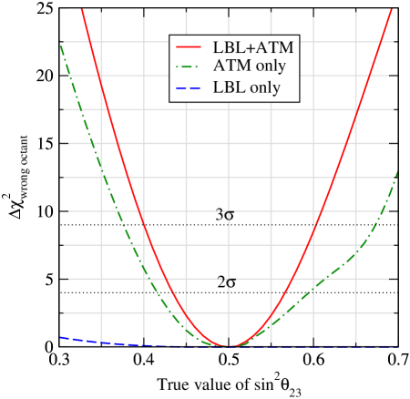
Building upon the results of Ref. [43] we show in Figure 2 the difference in $\chi^{2}$ between the true solution (with $\chi^{2}=0$) and the $\chi^{2}$-minimum in the wrong octant of $\theta_{23}$ ($(O^{\mathrm{wr}},H^{\mathrm{tr}})$-solution). It is clear form this figure that LBL data alone have no sensitivity at all to the octant of $\theta_{23}$, whereas ATM can reject the fake solution efficiently. Taking the combination of LBL+ATM data improves the sensitivity slightly, due to the more precise determination of other oscillation parameters by the LBL data. Using the combined LBL+ATM data the wrong octant can be rejected at 3$\sigma$ if $|\sin^{2}\theta_{23}-0.5|>0.1$. Let us note that the results shown in Figure 2 do hardly depend on our choice for the true neutrino mass ordering, thanks to $\theta_{13}^{\mathrm{true}}=0$. Non-zero values for $\theta_{13}^{\mathrm{true}}$ will be considered in Section 4.

3.3 The sensitivity of ATM data to the mass hierarchy

The determination of the ordering of the neutrino mass states is one of the most challenging tasks of future neutrino experiments. In long-baseline experiments the effects of $\theta_{13}$, $\delta_{\mathrm{CP}}$ and the sign of $\Delta m_{31}^{2}$ are highly entangled, and the determination of sign($\Delta m_{31}^{2}$) is probably only possible through the matter effect induced in an experiment with a very long baseline plus additional information from other LBL or reactor experiments [60, 61, 30, 23, 22, 13, 20, 62]. Therefore, the combined analysis of LBL and ATM data as offered from an oscillation experiment with a Mt water Cherenkov detector provides a very interesting possibility to answer the question of the neutrino mass hierarchy.

The sensitivity of atmospheric neutrino data to the neutrino mass hierarchy comes mainly from the modification of $e$-like multi-GeV events by earth matter effects for not too small values of $\sin^{2}2\theta_{13}$ [36, 39, 38, 37, 34, 35, 40]. Similar as in Eq. (9), one finds for the $\theta_{13}$ induced excess of $e$-like multi-GeV events

$$\epsilon_{e}^{\mathrm{multi}}\equiv\frac{N_{e}}{N_{e}^{0}}-1\approx\left(r\,\sin^{2}\theta_{23}-1\right)\langle P_{31}^{2\nu}\rangle\,.$$ (10)

Now $\langle P_{31}^{2\nu}\rangle$ is an effective two-flavor probability governed by $\Delta m_{31}^{2}$ and $\theta_{13}$, appropriately averaged and including the (weighted) contributions from neutrinos and anti-neutrinos. The effect is most pronounced for zenith angles corresponding to neutrino trajectories crossing the earth mantle, or earth mantle and core, where $\sin^{2}2\theta_{13}$-effects can be resonantly enhanced due to matter effects [33, 34, 35]. In the relevant zenith angle bins $\epsilon_{e}^{\mathrm{multi}}$ can reach values of the order of 10% (see e.g. Fig. 5 of Ref. [39]). Qualitatively $\epsilon_{e}^{\mathrm{multi}}$ shows the following behavior [39]:

• $\epsilon_{e}^{\mathrm{multi}}$ vanishes for $\sin^{2}2\theta_{13}=0$ and increases monotonically with $\sin^{2}2\theta_{13}$.

• For the normal hierarchy the resonant matter enhancement occurs for neutrinos, whereas for the inverted hierarchy it occurs for anti-neutrinos. Since the event numbers in water Cherenkov detectors are dominated by neutrinos because of larger cross sections (see Table 1), $\epsilon_{e}^{\mathrm{multi}}$ is larger by a factor of $1.5-2$ for the normal hierarchy than for the inverted one.

• Since in the multi-GeV range we have $r\simeq 2.6-4.5$, the factor $(r\,\sin^{2}\theta_{23}-1)$ in Eq. (10) suppresses the excess of $e$-like events for small values $\sin^{2}\theta_{23}\lesssim 0.4$, whereas larger values of $\sin^{2}\theta_{23}$ increase $\epsilon_{e}^{\mathrm{multi}}$. In particular, the effect is enhanced for $\theta_{23}>\pi/4$.

Therefore, if the true hierarchy is normal and $\theta_{23}<\pi/4$ there is only a small excess of $e$-like multi-GeV events, which can be accommodated to some extent with the inverted hierarchy. For the example point with $\sin^{2}\theta_{23}^{\mathrm{true}}=0.4$ chosen in the left panel of Figure 1 the wrong hierarchy can be disfavored only with a $\Delta\chi^{2}=5.0$. In contrast, for $\theta_{23}>\pi/4$ the excess of $e$-like events is enhanced by the flux-factor $(r\,\sin^{2}\theta_{23}-1)$. Therefore, a true normal hierarchy (resonant enhancement for neutrinos) plus the flux-factor enhancement leads to large values of $\epsilon_{e}^{\mathrm{multi}}$, which cannot be fitted with the inverted hierarchy (resonant enhancement for the smaller anti-neutrino sample). This explains the strong rejection of the wrong hierarchy solution in the right panel of Figure 1, with a $\Delta\chi^{2}=18.6$. We will discuss the mechanisms relevant for the rejection of the wrong hierarchy in more detail in Sections 4 and 5.

Finally we note that in addition to $\Delta m_{21}^{2}$-effects of Eq. (9) and $\theta_{13}$-effects of Eq. (10) also an interference term between the two contributions is present [44] (see also Ref. [53]). It is proportional to $(r\,\sin\theta_{13}\,\sin 2\theta_{23})$ and depends on the CP-phase $\delta_{\mathrm{CP}}$. Because of the different dependence on the flux ratio $r$ the interference term may become important in cases where the effects governed by Eqs. (9) and (10) are suppressed.

4 Resolving the degeneracies

Figure 3: Rejection of the fake solutions from LBL+ATM data as a function of the true values of $\sin^{2}2\theta_{13}$ and $\sin^{2}\theta_{23}$ for various $\delta_{\mathrm{CP}}^{\mathrm{true}}$ if the true hierarchy is normal (left) or inverted (right). Solid curves correspond to the solution with the wrong octant and the right hierarchy $(O^{\mathrm{wr}},H^{\mathrm{tr}})$, dashed curves to the right octant and the wrong hierarchy $(O^{\mathrm{tr}},H^{\mathrm{wr}})$, and shaded regions to the wrong octant and the wrong hierarchy $(O^{\mathrm{wr}},H^{\mathrm{wr}})$. We show the contours of $\Delta\chi^{2}=1,4,9$ between the fake and the true solution, corresponding to a rejection of the fake solution at the $1\sigma$, $2\sigma$, and $3\sigma$ CL (from light to dark shading) for 1 dof.

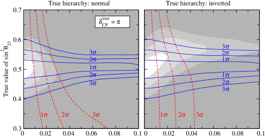
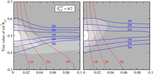
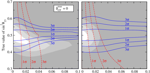
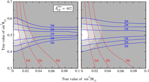
The examples shown in Figure 1 suggest that the LBL+ATM combination offers an efficient method to reject the degenerate solutions. To investigate this more systematically we have performed a scan over the true values for $\theta_{13}$ and $\theta_{23}$ and various values for $\delta_{\mathrm{CP}}^{\mathrm{true}}$. For a given point in the space of $\sin^{2}2\theta_{13}^{\mathrm{true}}$, $\sin^{2}\theta_{23}^{\mathrm{true}}$ and $\delta_{\mathrm{CP}}^{\mathrm{true}}$ we test the ability to rule out each of the three degenerate solutions $(O^{\mathrm{wr}},H^{\mathrm{tr}})$, $(O^{\mathrm{tr}},H^{\mathrm{wr}})$, and $(O^{\mathrm{wr}},H^{\mathrm{wr}})$. This is done by minimizing $\chi^{2}_{\mathrm{LBL+ATM}}$ with respect to all fit parameters, constraining the octant of $\theta_{23}$ and the sign of $\Delta m_{31}^{2}$ corresponding to the fake solution which we want to test. The results of this analysis are shown in Figure 3, which represents one of the main results of this work.

The solid curves in Figure 3 show that the $(O^{\mathrm{wr}},H^{\mathrm{tr}})$-solution corresponding to the $\theta_{23}$-degeneracy can be excluded at high confidence level if $\theta_{23}$ is far enough from $\pi/4$. (Note that if $\theta_{23}$ is close to $\pi/4$ this degeneracy disappears anyway.) For small values of $\sin^{2}2\theta_{13}^{\mathrm{true}}$ this follows mainly from the atmospheric sub-GeV $e$-like events, as discussed in Section 3.2. Moreover, if the true hierarchy is normal (left panels of Figure 3) we find an improvement of the octant sensitivity for $\sin^{2}2\theta_{13}\gtrsim 0.04$. This effect comes from the multi-GeV $e$-like events, where resonant enhancement occurs for sufficiently large $\sin^{2}2\theta_{13}$, and therefore an additional dependence on $\sin^{2}\theta_{23}$ appears according to Eq. (10). This can be seen from Figure 4, where we show the ability to reject the fake solutions using only sub-GeV (left) and multi-GeV (right) ATM data. The improvement for large $\sin^{2}2\theta_{13}$ is also visible for the inverted mass ordering (right panels of Figure 3), however, in that case the effect is much smaller, since the resonance occurs for anti-neutrinos in the inverted hierarchy, which contribute less to the total ATM data, and hence the significance of the effect is smaller than in the normal hierarchy, where the resonance occurs for neutrinos.

The wrong hierarchy solution $(O^{\mathrm{tr}},H^{\mathrm{wr}})$ can be excluded to the right of the dashed curves in Figure 3. We observe that the ability to reject this solution increases with $\sin^{2}\theta_{23}$. As discussed in Section 3.3 this follows from the fact that the excess of $e$-like multi-GeV events is enhanced for large $\sin^{2}\theta_{23}$. In particular, for $\sin^{2}\theta_{23}>0.5$ the sensitivity is completely dominated by multi-GeV data (compare Figure 4), and we observe a very small dependence on the true value of $\delta_{\mathrm{CP}}$ and on the true hierarchy. For $\sin^{2}\theta_{23}<0.5$ the situation becomes more complicated, and the sensitivity depends on the true value of $\delta_{\mathrm{CP}}$. In that region also sub-GeV data can contribute significantly, as visible in Figure 4. For low values of $\sin^{2}\theta_{23}$ the effect of multi-GeV data becomes suppressed by the flux factor $(r\sin^{2}\theta_{23}-1)$ in Eq. (10), and the contribution of sub-GeV data from Eq. (9) can become of comparable size. Moreover, as discussed in Ref. [44] for certain parameter values an interference term between the two contributions may become relevant, which depends on $\delta_{\mathrm{CP}}$. Therefore, the final sensitivity emerges from a rather involved interplay of various effects and ATM data samples.

Figure 4: Rejection of the fake solutions from LBL data combined with sub-GeV (left) and multi-GeV (right) $e$-like and $\mu$-like ATM data as a function of the true values of $\sin^{2}2\theta_{13}$ and $\sin^{2}\theta_{23}$ for $\delta_{\mathrm{CP}}^{\mathrm{true}}=0$ (upper) and $\delta_{\mathrm{CP}}^{\mathrm{true}}=-\pi/2$ (lower) and true normal hierarchy. Solid curves correspond to the solution with the wrong octant and the right hierarchy $(O^{\mathrm{wr}},H^{\mathrm{tr}})$, dashed curves to the right octant and the wrong hierarchy $(O^{\mathrm{tr}},H^{\mathrm{wr}})$, and shaded regions to the wrong octant and the wrong hierarchy $(O^{\mathrm{wr}},H^{\mathrm{wr}})$. We show the contours of $\Delta\chi^{2}=1,4,9$ between the fake and the true solution, corresponding to a rejection of the fake solution at the $1\sigma$, $2\sigma$, and $3\sigma$ CL (from light to dark shading) for 1 dof.

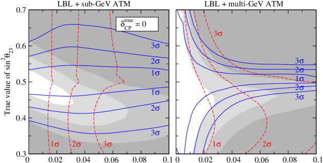
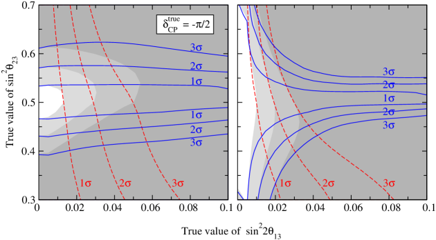
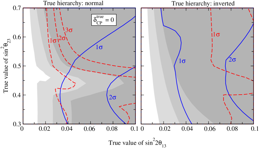
Finally, moving to the $(O^{\mathrm{wr}},H^{\mathrm{wr}})$-solution, we find that in most cases this “double” degenerate solution can be excluded if either the $(O^{\mathrm{wr}},H^{\mathrm{tr}})$- or the $(O^{\mathrm{tr}},H^{\mathrm{wr}})$-solution is ruled out. However, for certain parameter configurations an interesting degeneracy between the octant and the mass ordering appears, such that the $(O^{\mathrm{wr}},H^{\mathrm{wr}})$-solution cannot be excluded, although the $(O^{\mathrm{wr}},H^{\mathrm{tr}})$- and the $(O^{\mathrm{tr}},H^{\mathrm{wr}})$-solutions are not allowed. We find from Figure 3 that it is difficult to distinguish a normal mass hierarchy and $\sin^{2}\theta_{23}\simeq 0.45$, $\delta_{\mathrm{CP}}\simeq 0$ from an inverted hierarchy and $\sin^{2}\theta_{23}\simeq 0.55$, $\delta_{\mathrm{CP}}\simeq\pi$. We observe from the upper panels of Figure 4 that for these particular parameters sub-GeV as well as multi-GeV data cannot exclude the $(O^{\mathrm{wr}},H^{\mathrm{wr}})$-solution. However, the appearance of this remaining degeneracy strongly depends on the true value of $\delta_{\mathrm{CP}}$. For example, from the lower panels of Figure 4 it becomes clear that it does not occur for $\delta_{\mathrm{CP}}=-\pi/2$. The dependence on $\delta_{\mathrm{CP}}$ indicates that again the interference term between $\Delta m_{21}^{2}$- and $\theta_{13}$-effects is important.

5 Determining the neutrino mass hierarchy

In this section we discuss in detail the possibility to identify the type of the neutrino mass ordering from a combined LBL+ATM analysis. To this aim we simulate data for the T2K-II LBL experiment as well as for atmospheric neutrino data assuming a “true” neutrino mass ordering. Then we fit these data with the “wrong” hierarchy and search for the minimum $\chi^{2}$-value in the full 6-dimensional space of oscillation parameters, taking into account both $\theta_{23}$-degenerate solutions $(O^{\mathrm{tr}},H^{\mathrm{wr}})$ and $(O^{\mathrm{wr}},H^{\mathrm{wr}})$. If this minimum is larger than a certain value the wrong hierarchy can be excluded at the corresponding CL.

5.1 Sensitivity to the mass hierarchy for maximal $\theta_{23}$ mixing

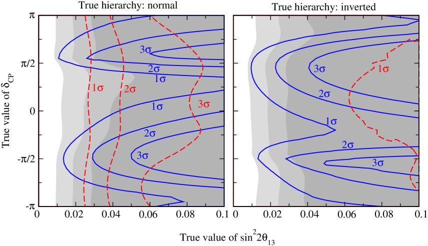
Before considering the general case we will first adopt the choice $\theta_{23}^{\mathrm{true}}=\pi/4$, such that the $\theta_{23}$-degeneracy is absent, and we are left only with the two-fold ambiguity related to sign($\Delta m_{31}^{2}$). We show the sensitivity to the hierarchy in Figure 5 as a function of the true values of $\sin^{2}2\theta_{13}$ and $\delta_{\mathrm{CP}}$. First we observe from this figure that the sensitivity of LBL data alone strongly depends on the true value of $\delta_{\mathrm{CP}}$. For certain values of $\delta_{\mathrm{CP}}$ the ability to distinguish normal and inverted hierarchy is even lost for $\sin^{2}2\theta_{13}=0.1$. The main reason for the difficulties of LBL alone to determine the mass hierarchy, is that for T2K-II the matter effect is very small. ATM data on their own allow to identify the normal mass hierarchy at $2\sigma$ CL for $\sin^{2}2\theta_{13}^{\mathrm{true}}\gtrsim 0.04$ (see left panel of Figure 5), whereas there is rather poor sensitivity to the inverted hierarchy (right panel of Figure 5). However, the sensitivity is significantly increased by combining the two data sets: For LBL+ATM data the wrong hierarchy can be excluded at $2\sigma$ CL for $\sin^{2}2\theta_{13}^{\mathrm{true}}\gtrsim 0.02$, with a rather small dependence on the true value of $\delta_{\mathrm{CP}}$ or the true type of the hierarchy.

Figure 5: Sensitivity to the mass hierarchy as a function of the true values of $\sin^{2}2\theta_{13}$ and $\delta_{\mathrm{CP}}$ for $\theta_{23}^{\mathrm{true}}=\pi/4$, if the true hierarchy is normal (left) or inverted (right). We show the contours of $\Delta\chi^{2}=1,4,9$ between the wrong and the true hierarchy, corresponding to a rejection of the wrong hierarchy at the $1\sigma$, $2\sigma$, and $3\sigma$ CL (from light to dark shading) for 1 dof. The shaded regions correspond to LBL+ATM data combined, solid curves correspond to LBL-only, and dashed curves to ATM-only.

These results can be understood qualitatively from the discussion given in Section 3.3. To achieve the same value of $\epsilon_{e}^{\mathrm{multi}}$ as implied by the (true) normal hierarchy and a given $\sin^{2}2\theta_{13}^{\mathrm{true}}$ with the inverted hierarchy, one has to adopt values of $\sin^{2}2\theta_{13}$ larger than $\sin^{2}2\theta_{13}^{\mathrm{true}}$ to increase the effect for the inverted hierarchy. Conversely, if the true hierarchy is inverted and one wants to fit $\epsilon_{e}^{\mathrm{multi}}$ with the normal ordering, $\sin^{2}2\theta_{13}$ has to be smaller than $\sin^{2}2\theta_{13}^{\mathrm{true}}$. This expectation is confirmed in Figure 6, where the allowed regions in the ($\sin^{2}2\theta_{13},\delta_{\mathrm{CP}}$) plane from ATM data are shown as dashed curves for the true values $\sin^{2}2\theta_{13}=0.03$ and $\delta_{\mathrm{CP}}=-0.85\pi$. The left panel shows that the normal hierarchy can be fitted with the inverted one for rather large values of $\sin^{2}2\theta_{13}$, whereas the opposite situation is visible for the inverted hierarchy in the right panel.

Figure 6: Allowed regions in the ($\sin^{2}2\theta_{13},\delta_{\mathrm{CP}}$) plane assuming for the true mass spectrum a normal (left) and an inverted (right) hierarchy, and $\theta_{23}^{\mathrm{true}}=\pi/4$. The true values $\sin^{2}2\theta_{13}^{\mathrm{true}}=0.03$ and $\delta_{\mathrm{CP}}^{\mathrm{true}}=-0.85\pi$ are marked by a star. The shaded areas and the solid curves correspond to the 1, 2, and 3 $\sigma$ allowed regions (2 dof) for the true and the sign($\Delta m^{2}_{31}$)-degenerate solution for LBL+ATM and LBL data, respectively. The dashed curves correspond to the $\Delta\chi^{2}$ contours of ATM data for the wrong sign of $\Delta m^{2}_{31}$. The $\Delta\chi^{2}$ of the best fit point with the wrong hierarchy for LBL+ATM data is given in the figure and its location is marked by a dot.

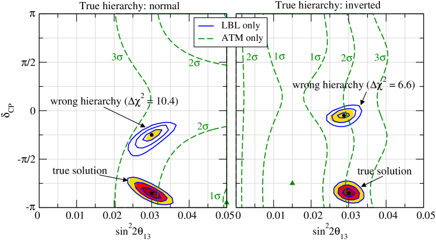
This behavior explains also the ATM-only results shown in Figure 5. The reasonable sensitivity of ATM data to the normal hierarchy visible in the left panel is given by the fact, that a fit with the inverted hierarchy would be only possible for very large values of $\sin^{2}2\theta_{13}$. This is disfavored by data, first because the values of $\sin^{2}2\theta_{13}$ required to fit the data start to get in conflict with the CHOOZ bound, and hence are disfavored, and second because such large values of $\sin^{2}2\theta_{13}$ start to be excluded from ATM data on their own. On the other hand the reason for the poor sensitivity to the inverted hierarchy shown in the right panel of Figure 5 is that in general small values of $\epsilon_{e}^{\mathrm{multi}}$ are expected, which can be easily fitted with the normal hierarchy but smaller $\sin^{2}2\theta_{13}$ (compare right panel of Figure 6), well below the sensitivity of ATM data.

Let us now discuss the effect of the sign($\Delta m_{31}^{2}$)-degeneracy for LBL data. In agreement with the discussion of Section 3.1 we observe from Figure 6 that the sign($\Delta m^{2}_{31}$) degeneracy affects mainly the determination of $\delta_{\mathrm{CP}}$, whereas the value of $\sin^{2}2\theta_{13}$ of the wrong-sign solution practically coincides with the true one. According to Eq. (8) we expect for the fake solution the value $\delta_{\mathrm{CP}}^{\prime}=-0.15\pi$, which is in good agreement with the values obtained in the actual fit: $\delta_{\mathrm{CP}}^{\prime}=-0.25(-0.05)\pi$ for true hierarchy normal (inverted). The deviations from the value of $\delta_{\mathrm{CP}}^{\prime}$ given by Eq. (8) are due to the matter effect, which is not included in the probability Eq. (3.1) and to some extent also to spectral information, which in general is difficult to include in the analytical discussion. Note that because of the choice $\theta_{23}^{\mathrm{true}}=\pi/4$ the $(O^{\mathrm{tr}},H^{\mathrm{wr}})$- and $(O^{\mathrm{wr}},H^{\mathrm{wr}})$-solutions coincide, and we are left only with the two-fold ambiguity implied by the sign($\Delta m_{31}^{2}$)-degeneracy, as visible in Figure 6.

From Figure 6 also the reason for the significant improvement of the sensitivity to the hierarchy for the LBL+ATM combination becomes clear. Although for LBL data alone the degenerate solution is present at a wrong value of $\delta_{\mathrm{CP}}$ even at $1\sigma$ CL, the value of $\sin^{2}2\theta_{13}$ has to be very similar to the true one. This makes it impossible to accommodate ATM data with the wrong hierarchy, since either values $\sin^{2}2\theta_{13}$ significantly larger or smaller than the true one are necessary to obtain the correct value for $\epsilon_{e}^{\mathrm{multi}}$ with the wrong hierarchy. The location in the ($\sin^{2}2\theta_{13},\delta_{\mathrm{CP}}$) plane required by the degenerate solution of LBL gives for ATM data a $\chi^{2}$ corresponding to $2-3\sigma$ CL. Therefore the combined data lead to the rather good sensitivity implied by the $\Delta\chi^{2}$-values given in Figure 6.

To summarize, the example shown in Figure 6 demonstrates how the combination of LBL and ATM data leads to a sensitivity to the mass hierarchy at the $3\sigma$ level, although each data set on its own cannot distinguish normal from inverted mass ordering for this particular choice of parameter values. The sensitivity of ATM data alone suffers from the fact that the wrong hierarchy can be accommodated by adjusting $\theta_{13}$, but also the parameters $\theta_{23}$, $\Delta m_{31}^{2}$, and $\delta_{\mathrm{CP}}$ are important. To benefit from the earth matter effects in $e$-like events from atmospheric neutrinos for the hierarchy determination the rather precise measurement of the oscillation parameters from LBL data is mandatory. In particular, it is necessary to know $\theta_{23}$ and $\Delta m_{31}^{2}$ at the 1% level, and a reasonable constraint on $\sin^{2}2\theta_{13}$ is required. Finally, the determination of the correct mass hierarchy through the LBL+ATM combination allows to resolve the ambiguity in $\delta_{\mathrm{CP}}$ from the sign($\Delta m_{31}^{2}$)-degeneracy, and hence the potential to measure $\delta_{\mathrm{CP}}$ is significantly increased. For the example shown in Figure 6 the correct value of $\delta_{\mathrm{CP}}$ can be identified at $2\sigma$ CL.

5.2 Sensitivity to the mass hierarchy for non-maximal $\theta_{23}$ mixing

Figure 7: Sensitivity to the mass hierarchy as a function of the true values of $\sin^{2}2\theta_{13}$ and $\sin^{2}\theta_{23}$ for $\delta_{\mathrm{CP}}^{\mathrm{true}}=0$ and a true normal (left panel) and inverted (right panel) hierarchy. We show the contours of $\Delta\chi^{2}=1,4,9$ between the wrong and the true hierarchy, corresponding to a rejection of the wrong hierarchy at the $1\sigma$, $2\sigma$, and $3\sigma$ CL (from light to dark shading) for 1 dof. The shaded regions correspond to LBL+ATM data combined, solid curves correspond to LBL-only, and dashed curves to ATM-only.

Now we generalize the discussion of the previous subsection to non-maximal values of $\theta_{23}^{\mathrm{true}}$, such that in general all four solutions of Eq. (2) are present. To identify the correct mass hierarchy the $(O^{\mathrm{tr}},H^{\mathrm{wr}})$- as well as the $(O^{\mathrm{wr}},H^{\mathrm{wr}})$-solution has to be excluded. In Figure 7 we show the sensitivity to the mass hierarchy as a function of the true values of $\sin^{2}2\theta_{13}$ and $\sin^{2}\theta_{23}$ for LBL, ATM, and LBL+ATM data. First we note that the results for LBL data-only strongly depend on the true value of $\delta_{\mathrm{CP}}$, as observed already in Figure 5. ATM data on their own provide only a reasonable sensitivity to the mass hierarchy if the true hierarchy is normal and $\sin^{2}\theta_{23}^{\mathrm{true}}>0.5$. This is the region of large excess of $e$-like multi-GeV events (see discussion in Section 3.3), which cannot be achieved for any configuration in the inverted hierarchy.

The sensitivity to the hierarchy for the LBL+ATM combination can be inferred from Figure 3 by considering the intersection of the shaded region ($(O^{\mathrm{wr}},H^{\mathrm{wr}})$-solution), with the region to the right of the dashed curves ($(O^{\mathrm{tr}},H^{\mathrm{wr}})$-solution). The shaded regions in Figure 7 give an explicit example for $\delta_{\mathrm{CP}}^{\mathrm{true}}=0$. For the true inverted hierarchy (right panel) the sensitivity to determine the mass hierarchy is given by the ability to exclude the $(O^{\mathrm{tr}},H^{\mathrm{wr}})$-solution. As discussed in Section 3 the worsening of the sensitivity for low values of $\sin^{2}\theta_{23}$ can be understood from the flux factor $(r\sin^{2}\theta_{23}-1)$ in the multi-GeV $e$-like event excess. If the true hierarchy is normal (left panel) the $(O^{\mathrm{tr}},H^{\mathrm{wr}})$- as well as the $(O^{\mathrm{wr}},H^{\mathrm{wr}})$-solutions have to be taken into account. The “spike” visible in Figure 7 at $\sin^{2}\theta_{23}^{\mathrm{true}}\sim 0.45$ comes from the fact that the double degenerate solution $(O^{\mathrm{wr}},H^{\mathrm{wr}})$ cannot be excluded.

Figure 8: Panel (a) shows the $\Delta\chi^{2}$ of the wrong hierarchy, panel (b) and (c) show the values of $\sin^{2}2\theta_{13}$ and $\sin^{2}\theta_{23}$ at the best fit point of the wrong hierarchy as a function of the true value of $\sin^{2}\theta_{23}$. The true hierarchy is normal and $\sin^{2}2\theta_{13}^{\mathrm{true}}=0.04$, $\delta_{\mathrm{CP}}^{\mathrm{true}}=0$.

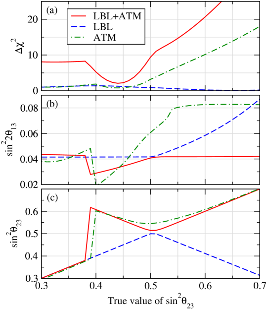
We illustrate this behavior in Figure 8, where we show the location of the best fit point for the wrong hierarchy as a function of the true value of $\sin^{2}\theta_{23}$. We observe from panel (c) that for $\sin^{2}\theta_{23}^{\mathrm{true}}>0.5$ the minimum for LBL+ATM follows the true value of $\sin^{2}\theta_{23}$, i.e., it corresponds to the $(O^{\mathrm{tr}},H^{\mathrm{wr}})$-solution. As discussed in Section 3 this implies in turn that $\sin^{2}2\theta_{13}$ has to be close to the true value, as can be seen from panel (b). However, in that case the large values of $\epsilon_{e}^{\mathrm{multi}}$ from the normal hierarchy cannot be obtained in the inverted hierarchy, which leads to the large $\chi^{2}$ values, i.e. good sensitivity, in that region. For $0.4<\sin^{2}\theta_{23}^{\mathrm{true}}<0.5$ one observes from Figure 8 that the best fit moves to the $(O^{\mathrm{wr}},H^{\mathrm{wr}})$-solution, characterized by the wrong $\theta_{23}$, see panel (c), and a value of $\sin^{2}2\theta_{13}$ given by Eq. (5), see panel (b). As mentioned in Section 4 the occurrence of this degeneracy strongly depends on the true value of $\delta_{\mathrm{CP}}$, and follows from a delicate interplay of effects in sub- and multi-GeV data. In the region of $\sin^{2}\theta_{23}^{\mathrm{true}}<0.4$ the best fit returns again to the $(O^{\mathrm{tr}},H^{\mathrm{wr}})$-solution, characterized by the true $\theta_{23}$ and a value of $\sin^{2}2\theta_{13}$ close to the true one. From Figure 8 we find that the fit of LBL-only, as well as ATM-only chooses best fit values of $\theta_{23}$ and $\sin^{2}2\theta_{13}$ close to the true ones. This suggests that in that region the sensitivity comes from effects related to $\Delta m_{31}^{2},\Delta m_{21}^{2}$, and $\delta_{\mathrm{CP}}$. As mentioned in Section 4 here the main sensitivity comes from the ATM sub-GeV data sample (compare Figure 4) and the interference term between $\Delta m_{21}^{2}$- and $\Delta m_{31}^{2}$-effects [44] can become important, which introduces the dependence on $\delta_{\mathrm{CP}}$.

Figure 9: Sensitivity to the mass hierarchy as a function of the true values of $\sin^{2}2\theta_{13}$ and $\delta_{\mathrm{CP}}$ for $\sin^{2}\theta_{23}^{\mathrm{true}}=0.3$ (left) and $\sin^{2}\theta_{23}^{\mathrm{true}}=0.7$ (right). The true hierarchy is normal. We show the contours of $\Delta\chi^{2}=1,4,9$ between the wrong and the true hierarchy, corresponding to a rejection of the wrong hierarchy at the $1\sigma$, $2\sigma$, and $3\sigma$ CL (from light to dark shading). The shaded regions correspond to LBL+ATM data combined, solid curves correspond to LBL-only, and dashed curves to ATM-only.

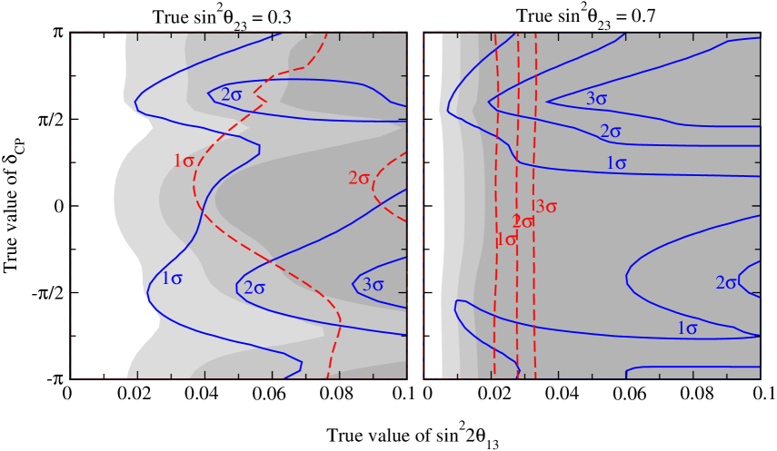
The strong dependence of the sensitivity on $\delta_{\mathrm{CP}}$ for small $\sin^{2}\theta_{23}$ is visible in the left panel of Figure 9, where we show the sensitivity to the hierarchy as a function of $\sin^{2}2\theta_{13}^{\mathrm{true}}$ and $\delta_{\mathrm{CP}}^{\mathrm{true}}$ for $\sin^{2}\theta_{23}^{\mathrm{true}}=0.3$. The rich structure visible for the LBL+ATM combination indicates a complicated interplay and/or cancellations of various effects. On the other hand, from the right panel we observe that for large values of $\sin^{2}\theta_{23}^{\mathrm{true}}$ the sensitivity to the hierarchy becomes practically independent of the true value of $\delta_{\mathrm{CP}}$. In this range multi-GeV $\Delta m_{31}^{2}$-effects are enhanced by the flux factor and dominate over $\Delta m_{21}^{2}$-effects and the interference term. Also ATM data alone provide quite a good sensitivity, thanks to the big effect in multi-GeV $e$-like events.

6 The $\theta_{23}$-degeneracy and the sensitivity to $\sin^{2}2\theta_{13}$

As discussed in Section 3, the presence of the octant degeneracy leads to severe complications in the determination of $\sin^{2}2\theta_{13}$. In this section we consider the specific case $\theta_{13}^{\mathrm{true}}=0$, and we investigate how the upper bound on $\sin^{2}2\theta_{13}$ (“sensitivity to $\sin^{2}2\theta_{13}$”) can be improved by the combined LBL+ATM analysis. The fact that the $\theta_{23}$-degeneracy affects the $\sin^{2}2\theta_{13}$-sensitivity is well-known, see e.g., Refs. [11, 13, 14, 16]. The choice $\theta_{13}^{\mathrm{true}}=0$ essentially eliminates the differences between normal and inverted hierarchies, i.e. the degeneracy is perfect, and the fact that it cannot be resolved introduces only very small ambiguities for other parameters. Hence the $(O^{\mathrm{wr}},H^{\mathrm{tr}})$- and $(O^{\mathrm{wr}},H^{\mathrm{wr}})$-solutions coincide within good accuracy. Moreover, the analysis is independent of the true value of $\delta_{\mathrm{CP}}$, since the phase becomes unphysical for $\theta_{13}=0$. We define the sensitivity to $\sin^{2}2\theta_{13}$ as the largest value of $\sin^{2}2\theta_{13}$ which fits the data generated for a true value $\sin^{2}2\theta_{13}^{\mathrm{true}}=0$ at a given CL (see Appendix C of Ref. [31] for a detailed discussion).

Figure 10: Sensitivity to $\sin^{2}2\theta_{13}$ as a function of the true value of $\sin^{2}\theta_{23}$ for LBL data only (dashed), and the combination LBL+ATM (solid). In panels (a) and (b) we restrict the fit of $\theta_{23}$ to the octant corresponding to $\theta_{23}^{\mathrm{true}}$ and $\pi/2-\theta_{23}^{\mathrm{true}}$, respectively, whereas panel (c) shows the overall sensitivity taking into account both octants.

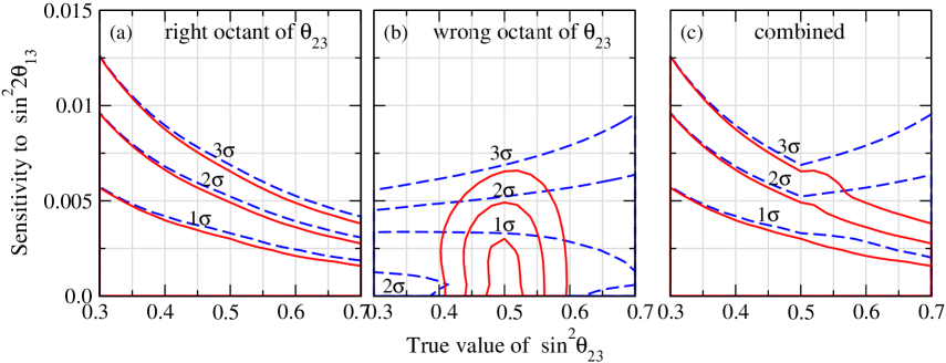
Let us first assume that the true octant of $\theta_{23}$ was known. In that case one expects from Eq. (3.1) that the sensitivity for $\sin^{2}2\theta_{13}$ becomes better for increasing $\sin^{2}\theta_{23}$, since for large $\sin^{2}\theta_{23}$ the first term in Eq. (3.1), which is proportional to $\sin^{2}2\theta_{13}$, is enhanced. Moreover, the $\alpha^{2}$ term gets suppressed for small $\cos^{2}\theta_{23}$, which reduces the effect of multi-parameter correlations induced by $\Delta m_{21}^{2}$. This expectation is confirmed in panel (a) of Figure 10, where the sensitivity to $\sin^{2}2\theta_{13}$ is shown as a function of the true value of $\sin^{2}\theta_{23}$, assuming that the octant is known. However, if the octant of $\theta_{23}$ is not known, the degenerate solution prevents the smaller $\sin^{2}2\theta_{13}$-limits implied by $\sin^{2}\theta_{23}^{\mathrm{true}}>0.5$. In that case the data can be fitted by relatively large values of $\sin^{2}2\theta_{13}$, since exchanging $\sin^{2}\theta_{23}$ and $\cos^{2}\theta_{23}$ reduces the effect of $\sin^{2}2\theta_{13}$ and increases the $\alpha^{2}$ term in Eq. (3.1). This effect is shown by the curves corresponding to LBL data in panel (c) of Figure 10. We observe that the sensitivity to $\sin^{2}2\theta_{13}$ gets worse for non-maximal values of $\theta_{23}^{\mathrm{true}}$ in both octants because of the presence of the degenerate solution.

Since the octant-degeneracy can be efficiently resolved by atmospheric data one expects a significant improvement of the $\sin^{2}2\theta_{13}$-sensitivity for the combined LBL+ATM analysis. In panel (b) of Figure 10 we show the $\sin^{2}2\theta_{13}$-limit constraining the fit to the wrong octant of $\theta_{23}$. As expected from Figure 2 there are no solutions for LBL+ATM data if $\theta_{23}$ is sufficiently far from maximal, since the wrong solution is disfavored by ATM data. Consequently, we find that the final result shown in panel (c) for LBL+ATM is very close to the situation in panel (a), where only the true solution for $\theta_{23}$ has been used. Hence, the $\sin^{2}2\theta_{13}$-sensitivity is significantly increased for $\theta_{23}>\pi/4$ through the exclusion of the wrong octant solution by ATM data. There is no relevant improvement for $\theta_{23}<\pi/4$, since in that case the sensitivity to $\sin^{2}2\theta_{13}$ suffers for the true $\theta_{23}$ solution because of the $\sin^{2}2\theta_{13}$-suppression implied by the small values of $\sin^{2}\theta_{23}$.

7 Conclusions

In this work we have performed a combined analysis of future long-baseline (LBL) and atmospheric (ATM) neutrino data. As a specific example we have considered the phase II of the T2K experiment, consisting of a 4 MW superbeam produced at the J-PARC facility. The 1 Mt HyperKamiokande water Cherenkov detector will serve as detector for the LBL experiment and simultaneously provide high statistics ATM neutrino data. We have shown that the combined LBL+ATM analysis offers a very appealing possibility to resolve parameter degeneracies in the LBL data. In particular, the ambiguities implied by the sign($\Delta m_{31}^{2}$)- and the $\theta_{23}$-degeneracies can be lifted to a large extent. This becomes possible through three-flavor effects in ATM data related to $\theta_{13}$ and $\Delta m_{21}^{2}$. A systematic scan of the parameter space has been performed to investigate the ability to determine the type of the neutrino mass ordering. Let us summarize our main findings:

• For true values of $\sin^{2}\theta_{23}>0.5$ the correct mass hierarchy can be identified at $2\sigma$ CL if $\sin^{2}2\theta_{13}\gtrsim 0.015$, rather independent of the true value of $\delta_{\mathrm{CP}}$ or the type of the true hierarchy. In this region the sensitivity is dominated by multi-GeV $e$-like events in ATM data.

• For true values of $\sin^{2}\theta_{23}<0.5$ the correct mass hierarchy can be identified at $2\sigma$ CL if $\sin^{2}2\theta_{13}\gtrsim 0.03$, where here the actual sensitivity depends on the true value of $\delta_{\mathrm{CP}}$ and the true hierarchy. The final sensitivity emerges from an interplay of various effects in the different ATM data samples.

• The solution with the wrong octant of $\theta_{23}$ can be excluded at $3\sigma$ CL if $|\sin^{2}\theta_{23}-0.5|\gtrsim 0.1$, independent of the true values of $\theta_{13}$, $\delta_{\mathrm{CP}}$, and the hierarchy. This follows mainly from $\Delta m_{21}^{2}$-effects in $e$-like sub-GeV ATM data. If $\sin^{2}2\theta_{13}\gtrsim 0.03$ and the true hierarchy is normal the octant sensitivity at $3\sigma$ CL improves to $|\sin^{2}\theta_{23}-0.5|\gtrsim 0.05$ due to $\theta_{13}$-effects in the multi-GeV ATM data.

• The lifting of the degeneracies by ATM data significantly increases the performance of the LBL experiment for the measurement of $\sin^{2}2\theta_{13}$ and $\delta_{\mathrm{CP}}$, since fake solutions implied by the degeneracies can be ruled out. Generically, the determination of the correct octant of $\theta_{23}$ removes an ambiguity in the measurement of $\sin^{2}2\theta_{13}$, whereas lifting the sign($\Delta m_{31}^{2}$)-degeneracy allows the identification of the correct value of $\delta_{\mathrm{CP}}$.

• If no finite value for $\theta_{13}$ is found the upper limit on $\sin^{2}2\theta_{13}$ is significantly improved by resolving the $\theta_{23}$-degeneracy by ATM data if $\theta_{23}>\pi/4$.

Let us stress that these results follow from the complementarity of the two data sets; neither LBL data alone nor ATM data alone can provide a comparable physics reach. The LBL data allow a very precise determination of $|\Delta m_{31}^{2}|$ and $\sin^{2}2\theta_{23}$, and although $\theta_{13}$ and $\delta_{\mathrm{CP}}$ suffer from ambiguities related to the degeneracies they are constrained to rather specific values. However, there is very poor sensitivity to the mass hierarchy and to the octant of $\theta_{23}$ for LBL data alone. For ATM data alone only for $\sin^{2}\theta_{23}^{\mathrm{true}}\gtrsim 0.6$ and a true normal hierarchy a reasonable sensitivity exists for the mass ordering, since in this case a big excess of $e$-like multi-GeV events is predicted, which cannot be achieved by any configuration within the inverted hierarchy. For all other regions in the parameter space the sensitivity of ATM-only is rather poor, since the data can be fitted with the wrong hierarchy by adjusting the oscillation parameters. To benefit from the hierarchy sensitivity offered by $\theta_{13}$-earth matter effects in ATM data the precise measurement of the oscillation parameters from LBL data is mandatory. In particular, it is necessary to know $\theta_{23}$ and $|\Delta m_{31}^{2}|$ at the 1% level, and a reasonable constraint on $\sin^{2}2\theta_{13}$ is required. Hence, only the combination of LBL and ATM data makes it possible to obtain a good sensitivity to the neutrino mass hierarchy. Let us add that to benefit from the LBL+ATM combination indeed a few $\mathrm{Mt\,yrs}$ of ATM data are necessary. In particular we have checked that for exposures below $1\,\mathrm{Mt\,yrs}$ the sensitivity to the hierarchy is essentially lost.

Finally, let us remark that the methods to resolve parameter degeneracies discussed previously in general involve the combination of two or more (expensive) experiments, e.g. at different baselines or using different oscillation channels. In contrast, once a LBL experiment with a megaton Cherenkov detector is built, ATM data come for free. Therefore, in addition to the interesting physics, the synergies between LBL and ATM data offer a relatively economical way of resolving parameter degeneracies.

Acknowledgment

M.M. is supported by the National Science Foundation grant PHY-0354776. T.S. is supported by the VI Framework Programme of the European Community under a Marie Curie Intra-European Fellowship.

References

- [1] S. N. Ahmed et al. (SNO), Phys. Rev. Lett. 92, 181301 (2004), nucl-ex/0309004; S. Fukuda et al. (Super-Kamiokande), Phys. Lett. B539, 179 (2002), hep-ex/0205075; B. T. Cleveland et al., Astrophys. J. 496, 505 (1998); J. N. Abdurashitov et al. (SAGE), J. Exp. Theor. Phys. 95, 181 (2002); M. Altmann et al. (GNO), Phys. Lett. B490, 16 (2000), hep-ex/0006034.
- [2] Y. Fukuda et al. (Super-Kamiokande), Phys. Rev. Lett. 81, 1562 (1998), hep-ex/9807003; M. Sanchez et al. (Soudan 2), Phys. Rev. D68, 113004 (2003), hep-ex/0307069; M. Ambrosio et al. (MACRO), Eur. Phys. J. C36, 323 (2004).
- [3] T. Araki et al. (KamLAND) (2004), hep-ex/0406035; M. Apollonio et al. (CHOOZ), Eur. Phys. J. C27, 331 (2003), hep-ex/0301017; F. Boehm et al. (Palo Verde), Phys. Rev. D64, 112001 (2001), hep-ex/0107009.
- [4] E. Aliu (K2K) (2004), hep-ex/0411038.
- [5] M. Maltoni, T. Schwetz, M. A. Tortola, and J. W. F. Valle, New J. Phys. 6, 122 (2004), hep-ph/0405172.
- [6] E. Ables et al. (MINOS) FERMILAB-PROPOSAL-P-875; P. Aprili et al. (ICARUS) CERN-SPSC-2002-027; D. Duchesneau (OPERA), eConf C0209101, TH09 (2002), hep-ex/0209082.
- [7] K. Anderson et al. (2004), White paper report on using nuclear reactors to search for a value of , hep-ex/0402041; F. Ardellier et al. (2004), Letter of intent for Double-CHOOZ, hep-ex/0405032.
- [8] J. J. Gomez-Cadenas et al. (CERN working group on Super Beams), Nucl. Phys. B646, 321 (2001), hep-ph/0105297; I. Ambats et al. (NOvA) FERMILAB-PROPOSAL-0929; M. V. Diwan et al., Phys. Rev. D68, 012002 (2003), hep-ph/0303081.
- [9] Y. Itow et al., Nucl. Phys. B, Proc. Suppl. 111, 146 (2001), The JHF-Kamioka neutrino project, hep-ex/0106019.
- [10] C. Albright et al. (Neutrino Factory/Muon Collider) (2004), physics/0411123.
- [11] V. Barger, D. Marfatia, and K. Whisnant, Phys. Rev. D65, 073023 (2002), hep-ph/0112119.
- [12] M. Freund, P. Huber, and M. Lindner, Nucl. Phys. B615, 331 (2001), hep-ph/0105071.
- [13] P. Huber, M. Lindner, and W. Winter, Nucl. Phys. B645, 3 (2002), hep-ph/0204352.
- [14] A. Donini, D. Meloni, and S. Rigolin, JHEP 06, 011 (2004), hep-ph/0312072.
- [15] M. Aoki, K. Hagiwara, and N. Okamura (2003), hep-ph/0311324.
- [16] O. Yasuda, New J. Phys. 6, 83 (2004), hep-ph/0405005.
- [17] H. Minakata, H. Nunokawa, and S. J. Parke, Phys. Rev. D66, 093012 (2002), hep-ph/0208163.
- [18] M. Koike, T. Ota, and J. Sato, Phys. Rev. D65, 053015 (2002), hep-ph/0011387.
- [19] J. Burguet-Castell, M. B. Gavela, J. J. Gomez-Cadenas, P. Hernandez, and O. Mena, Nucl. Phys. B608, 301 (2001), hep-ph/0103258.
- [20] H. Minakata and H. Nunokawa, JHEP 10, 001 (2001), hep-ph/0108085.
- [21] G. L. Fogli and E. Lisi, Phys. Rev. D54, 3667 (1996), hep-ph/9604415.
- [22] P. Huber, M. Lindner, and W. Winter, Nucl. Phys. B654, 3 (2003), hep-ph/0211300.
- [23] P. Huber and W. Winter, Phys. Rev. D68, 037301 (2003), hep-ph/0301257.
- [24] A. Cervera et al., Nucl. Phys. B579, 17 (2000), hep-ph/0002108.
- [25] V. Barger, D. Marfatia, and K. Whisnant, Phys. Rev. D66, 053007 (2002), hep-ph/0206038.
- [26] J. Burguet-Castell, D. Casper, J. J. Gomez-Cadenas, P. Hernandez, and F. Sanchez, Nucl. Phys. B695, 217 (2004), hep-ph/0312068.
- [27] A. Donini, D. Meloni, and P. Migliozzi, Nucl. Phys. B646, 321 (2002), hep-ph/0206034; D. Autiero et al., Eur. Phys. J. C33, 243 (2004), hep-ph/0305185.
- [28] H. Minakata, H. Sugiyama, O. Yasuda, K. Inoue, and F. Suekane, Phys. Rev. D68, 033017 (2003), hep-ph/0211111.
- [29] H. Minakata and H. Sugiyama, Phys. Lett. B580, 216 (2004), hep-ph/0309323.
- [30] P. Huber, M. Lindner, T. Schwetz, and W. Winter, Nucl. Phys. B665, 487 (2003), hep-ph/0303232.
- [31] P. Huber, M. Lindner, M. Rolinec, T. Schwetz, and W. Winter, Phys. Rev. D70, 073014 (2004), hep-ph/0403068.
- [32] K. B. McConnel and M. H. Shaevitz (2004), hep-ex/0409028.
- [33] L. Wolfenstein, Phys. Rev. D17, 2369 (1978); S. P. Mikheev and A. Y. Smirnov, Sov. J. Nucl. Phys. 42, 913 (1985).
- [34] S. T. Petcov, Phys. Lett. B434, 321 (1998), hep-ph/9805262.
- [35] E. K. Akhmedov, Nucl. Phys. B538, 25 (1999), hep-ph/9805272.
- [36] E. K. Akhmedov, A. Dighe, P. Lipari, and A. Y. Smirnov, Nucl. Phys. B542, 3 (1999), hep-ph/9808270.
- [37] M. Chizhov, M. Maris, and S. T. Petcov (1998), hep-ph/9810501; M. V. Chizhov and S. T. Petcov, Phys. Rev. Lett. 83, 1096 (1999), hep-ph/9903399; Phys. Rev. D63, 073003 (2001), hep-ph/9903424.
- [38] J. Bernabeu, S. Palomares-Ruiz, A. Perez, and S. T. Petcov, Phys. Lett. B531, 90 (2002), hep-ph/0110071.
- [39] J. Bernabeu, S. Palomares Ruiz, and S. T. Petcov, Nucl. Phys. B669, 255 (2003), hep-ph/0305152.
- [40] T. Kajita, Talk at NOON2004, February 11-15, 2004, Tokyo, Japan, http://www-sk.icrr.u-tokyo.ac.jp/noon2004.
- [41] C. W. Kim and U. W. Lee, Phys. Lett. B444, 204 (1998), hep-ph/9809491.
- [42] O. L. G. Peres and A. Y. Smirnov, Phys. Lett. B456, 204 (1999), hep-ph/9902312.
- [43] M. C. Gonzalez-Garcia, M. Maltoni, and A. Y. Smirnov, Phys. Rev. D70, 093005 (2004), hep-ph/0408170.
- [44] O. L. G. Peres and A. Y. Smirnov, Nucl. Phys. B680, 479 (2004), hep-ph/0309312.
- [45] RCCN Workshop on sub-dominant oscillation effects in atmospheric neutrino experiments, Dec 9-11, 2004, Kashiwa, Japan, http://www-rccn.icrr.u-tokyo.ac.jp/rccnws04/.
- [46] The UNO whitepaper, ‘Physics Potential and Feasibility of UNO’, SBHEP01-3 (2001), available at http://ale.physics.sunysb.edu/uno/.
- [47] L. Mosca, Talk at ‘Physics with a Multi-MW Proton Source’, CERN, Geneva, 25–27 May 2004, available at http://physicsatmwatt.web.cern.ch/physicsatmwatt/.
- [48] T. Tabarelli de Fatis, Eur. Phys. J. C24, 43 (2002), hep-ph/0202232; G. Rajasekaran (2004), hep-ph/0402246; S. Palomares-Ruiz and S. T. Petcov (2004), hep-ph/0406096; D. Indumathi and M. V. N. Murthy (2004), hep-ph/0407336.
- [49] P. Huber, M. Lindner, and W. Winter (2004), hep-ph/0407333; GLoBES webpage: http://www.ph.tum.de/globes/.
- [50] O. Yasuda (1996), hep-ph/9602342; (1997), hep-ph/9706546.
- [51] G. L. Fogli, E. Lisi, and A. Marrone, Phys. Rev. D64, 093005 (2001), hep-ph/0105139.
- [52] M. C. Gonzalez-Garcia and M. Maltoni, Eur. Phys. J. C26, 417 (2003), hep-ph/0202218.
- [53] E. Lisi (2004), Talk at Ref. [45].
- [54] M. C. Gonzalez-Garcia and M. Maltoni, Phys. Rev. D70, 033010 (2004), hep-ph/0404085.
- [55] M. Honda, T. Kajita, K. Kasahara, and S. Midorikawa, Phys. Rev. D70, 043008 (2004), astro-ph/0404457.
-
[56]
P. Huber
(2003), PhD thesis, available at
http://www.ph.tum.de/lehrstuehle/T30d/papers/huber2.pdf. - [57] S. Antusch, P. Huber, J. Kersten, T. Schwetz, and W. Winter, Phys. Rev. D70, 097302 (2004), hep-ph/0404268.
- [58] H. Minakata, M. Sonoyama, and H. Sugiyama (2004), hep-ph/0406073.
- [59] S. Antusch, J. Kersten, M. Lindner, and M. Ratz, Nucl. Phys. B674, 401 (2003), hep-ph/0305273.
- [60] V. D. Barger, S. Geer, R. Raja, and K. Whisnant, Phys. Lett. B485, 379 (2000), hep-ph/0004208.
- [61] P. Lipari, Phys. Rev. D61, 113004 (2000), hep-ph/9903481.
- [62] O. Mena and S. Parke, Phys. Rev. D70, 093011 (2004), hep-ph/0408070.
- [63] M. Kachelriess and R. Tomas (2004), hep-ph/0412100.