Mixing and decays of the antidecuplet in the context of approximate SU(3) symmetry

Abstract

We consider mixing of the antidecuplet with three $J^{P}=1/2^{+}$ octets (the ground-state octet, the octet containing $N(1440)$, $\Lambda(1600)$, $\Sigma(1660)$ and $\Xi(1690)$ and the octet containing $N(1710)$, $\Lambda(1800)$, $\Sigma(1880)$ and $\Xi(1950)$) in the framework of approximate flavor SU(3) symmetry. We give general expressions for the partial decay widths of all members of the antidecuplet as functions of the two mixing angles. Identifying $N_{\overline{10}}$ with the $N(1670)$ observed by the GRAAL experiment, we show that the considered mixing scenario can accommodate all present experimental and phenomenological information on the $\Theta^{+}$ and $N_{\overline{10}}$ decays: $\Theta^{+}$ could be as narrow as 1 MeV; the $N_{\overline{10}}\to N\,\eta$ decay is sizable, while the $N_{\overline{10}}\to N\,\pi$ decay is suppressed and the $N_{\overline{10}}\to\Lambda\,K$ decay is possibly suppressed. Constraining the mixing angles by the $N_{\overline{10}}$ decays, we make definite predictions for the $\Sigma_{\overline{10}}$ decays. We point out that $\Sigma_{\overline{10}}$ with mass near 1770 MeV could be searched for in the available data on $K_{S}\,p$ invariant mass spectrum, which already revealed the $\Theta^{+}$ peak. It is important to experimentally verify the decay properties of $\Sigma(1770)$ because its mass and $J^{P}=1/2^{+}$ make it an attractive candidate for $\Sigma_{\overline{10}}$.

I Introduction

Approximate flavor SU(3) symmetry of strong interactions predicts that hadrons are grouped into certain multiplets (families) Eightfoldway : Singlets, octets ($\bf{8}$), decuplets ($\bf{10}$), antidecuplets ($\bf{\overline{10}}$), 27-plets, 35-plets, etc. It is a piece of textbook wisdom that all known hadrons, which can constitute of three quarks, can be successively placed into singlets, octets and decuplets Kokkedee ; Close ; Samios74 and that other (higher) SU(3) representations are not required. The discoveries of the $\Theta^{+}$ SPRING8 ; DIANA ; CLAS ; SAPHIR ; Neutrino ; CLAS2 ; HERMES ; SVD ; COSYTOF ; ZEUS ; GRAAL ; Togoo ; Troyan and $\Xi_{3/2}$ NA49 , if confirmed BES ; ALEPH ; BABAR ; HERAB ; CDF ; FOCUS ; Belle ; PHENIX , mean the existence of the whole new exotic family – the antidecuplet.

In QCD and in Nature, SU(3) is broken by non-equal masses of the up, down and strange quarks. As a result, members of different SU(3) multiplets of the same spin and parity can mix. If the antidecuplet has indeed $J^{P}=1/2^{+}$ as predicted in the chiral quark-soliton approach DPP , then the antidecuplet can potentially mix with three known $J^{P}=1/2^{+}$ octets and with a $J^{P}=1/2^{+}$ decuplet. In addition to the traditional SU(3) multiplets, the antidecuplet can also mix with a 27-plet and a 35-plet 27plet .

The degree of mixing due to SU(3) violation among SU(3) multiplets, especially in the baryon sector, cannot be large in order for the notion of approximate SU(3) symmetry to make sense. However, in the meson sector, there are known exceptions from small mixing because of the accidental degeneracy in mass of a singlet and an octet member. The most celebrated example is the large (ideal) mixing between the $\phi$ and $\omega$ vector mesons Eightfoldway ; Kokkedee .

In our analysis, we consider the mixing angles (the parameters which describe the mixing) as small parameters. Because of the small width of the $\Theta^{+}$ PWA ; Nussinov ; Heidenbauer ; Cahn ; Gibbs ; Sibirtsev ; Sibirtsev2 , small mixing with the antidecuplet does not affect the properties of the involved octets. However, the decays of the ${\bf\overline{10}}$ members dramatically depend on even very small mixing.

In this work, we examine the scenario that the antidecuplet mixes simultaneously with three octets – with the ground-state octet, with the octet containing $N(1440)$, $\Lambda(1600)$, $\Sigma(1660)$ and $\Xi(1690)$, and with the octet containing $N(1710)$, $\Lambda(1800)$, $\Sigma(1880)$ and $\Xi(1950)$ – and with a 27-plet and a 35-plet. The coupling constants and the mixing angles with the ground-state octet and with the 27-plet and 35-plet are taken from the chiral quark soliton model 27plet . For the other two octets, the coupling constants are determined from the $\chi^{2}$ fit to the available decay widths, and the two corresponding mixing angles are left as free parameters.

This strategy enables us to present the general expressions for the $\overline{10}\to B+P$ decay widths, where $B$ is the ground-state baryon and $P$ is the ground-state pseudoscalar meson, as functions of the two mixing angles, the total width of the $\Theta^{+}$ and the pion-nucleon sigma term. Using scarce experimental information on the observation, non-observation and decays of the members of the antidecuplet, we give most probable regions of the mixing angles and make predictions for the yet unmeasured decay modes of the ${\bf\overline{10}}$. This enables us to suggest the reactions most favorable for the excitation and identification of the members of the antidecuplet.

II Antidecuplet mixing with three octets and $\overline{10}\to B+P$ decays

II.1 General formalism

We examine the scenario that the antidecuplet mixes simultaneously with three octets. The mixing takes place through the $N$-like and $\Sigma$-like states of the involved multiplets. The physical octet $|N_{1}^{\rm phys}\rangle$, $|N_{2}^{\rm phys}\rangle$, $|N_{3}^{\rm phys}\rangle$ and the antidecuplet $|N_{\overline{10}}^{\rm phys}\rangle$ states can be expressed in terms of the octet states, $|N_{1}\rangle$, $|N_{2}\rangle$ and $|N_{3}\rangle$, and the purely antidecuplet $|N_{\overline{10}}\rangle$ state,

$$\left(\begin{array}[]{c}|N_{1}^{\rm phys}\rangle\\ |N_{2}^{\rm phys}\rangle\\ |N_{3}^{\rm phys}\rangle\\ |N_{\overline{10}}^{\rm phys}\rangle\\ \end{array}\right)=\left(\begin{array}[]{cccc}1&0&0&\sin\theta_{1}\\ 0&1&0&\sin\theta_{2}\\ 0&0&1&\sin\theta_{3}\\ -\sin\theta_{1}&-\sin\theta_{2}&-\sin\theta_{3}&1\\ \end{array}\right)\left(\begin{array}[]{c}|N_{1}\rangle\\ |N_{2}\rangle\\ |N_{3}\rangle\\ |N_{\overline{10}}\rangle\\ \end{array}\right)\,,$$ (1)

assuming that the $\theta_{1}$, $\theta_{2}$ and $\theta_{3}$ mixing angles are small. A similar equation relates the physical $|\Sigma_{1}^{\rm phys}\rangle$, $|\Sigma_{2}^{\rm phys}\rangle$, $|\Sigma_{3}^{\rm phys}\rangle$ and $|\Sigma_{\overline{10}}^{\rm phys}\rangle$ states to the octet $|\Sigma_{1}\rangle$, $|\Sigma_{2}\rangle$, $|\Sigma_{3}\rangle$ states and the purely antidecuplet $|\Sigma_{\overline{10}}\rangle$ state after the replacement $\theta_{i}\to\theta_{i}^{\Sigma}$.

In our analysis, we assume that the $\theta_{i}$ mixing angles are small, $\sin\theta_{i}={\cal O}(\epsilon)$. The small parameter $\epsilon$ describes not only the violation of flavor SU(3) symmetry due to the non-zero mass of the strange quark, but also a possible additional dynamical suppression of the mixing between exotic and non-exotic states. In addition, the smallness of $\theta_{i}$ rests on the previous phenomenological analyses of non-exotic baryon multiplets, which observed only small mixing angles, see e.g. Samios74 .

In our analysis, we systematically neglect ${\cal O}(\epsilon^{2})$ terms. Therefore, the mixing matrix in Eq. (1) is unitary up to ${\cal O}(\epsilon^{2})$ corrections.

It is important to note that, in general, the $|N_{1}\rangle$, $|N_{2}\rangle$ and $|N_{3}\rangle$ states can mix among themselves. Indeed, our analysis GPreview shows that the $|N_{2}\rangle$ and $|N_{3}\rangle$ states are slightly mixed and that the $|N_{1}\rangle$ state can be considered as a pure state (it does not have components from other SU(3) multiplets). Therefore, in practice the problem of mixing of the antidecuplet with the three octets is solved in two steps. First, we determine the SU(3) coupling constants and the mixing angles for the three octets. Because of the smallness of $\Gamma_{\Theta^{+}}$ and $\theta_{i}$, it is legitimate to neglect the antidecuplet admixture at this stage. Details of this analysis are presented in Appendix A. Second, the resulting octet states are mixed with the antidecuplet states. Naturally, since the possible mixing among the octets was already been taken into account in step one, it is sufficient to consider only the mixing of each individual $|N_{i}^{\rm phys}\rangle$ ($i=1,2,3$) with $|N_{\overline{10}}^{\rm phys}\rangle$ – see Eq. (1). The same procedure applies to the considered octet and antidecuplet $\Sigma$ states.

The assumption of small mixing angles with the antidecuplet is in stark contrast with the quark model calculations JW ; Stancu , which automatically lead to almost ideal  mixing Faiman ; Cohen . Indeed, eigenstates of a generic quark model Hamiltonian have separately almost well-defined number of strange quarks and strange antiquarks. In the language of approximate flavor SU(3) symmetry, this can be realized only by almost ideal mixing of SU(3) states, which contain both non-strange and hidden strange components, such that the states resulting after the mixing contain mostly either non-strange quarks or strange quarks.

Of course, both small mixing and large mixing scenarios are assumptions which must be confronted with the data. A straightforward $\chi^{2}$ analysis of the available $N(1440)$ and $N(1710)$ partial decays widths shows that the popular scenario of Jaffe and Wilczek JW , which assumes nearly ideal mixing of $N(1440)$ (mostly octet state) with $N(1710)$ (mostly antidecuplet state), is inconsistent with the experimental data on the $N(1440)$ and $N(1710)$ decays PDG : It is impossible to simultaneously accommodate $\Gamma_{\Theta^{+}}\leq 10$ MeV and a large $\Gamma_{N(1440)\to N\,\pi}$. The same conclusion, but without the $\chi^{2}$ fit, was obtained in DP2004 ; Cohen .

The physical states are eigenstates of the mass operator $\hat{M}$. The corresponding physical masses $N_{i}^{\rm phys}$ are

$$N_{i}^{\rm phys}\equiv\langle N_{i}^{\rm phys}|\hat{M}|N_{i}^{\rm phys}\rangle=N_{i}+\sin^{2}\theta_{i}N_{\overline{10}}=N_{i}+{\cal O}(\epsilon^{2})\,,$$ (2)

where $N_{i}$ is the mass of the unmixed $|N_{i}\rangle$ state and $i=1,2,3,\overline{10}$. Thus, to the leading order in the SU(3)-violation effect, the physical masses are equal to the corresponding masses of the unmixed states. This means that the Gell-Mann–Okubo mass formulas are not sensitive to the small mixing, if it is treated consistently. Keeping only terms linear in the mass of the strange quark, it is not legitimate to estimate the mixing angles from the Gell-Mann–Okubo mass splitting formula, as was done for instance in DP2004 . Instead, as will be shown below, one has to consider decays since, in the presence of multiplet mixing, the decay widths contain a first power of the mixing angles.

Since the mechanism of the mixing of the $N$-states and $\Sigma$-states is the same, the mixing angles $\theta_{i}$ and $\theta_{i}^{\Sigma}$ are related DP2004

$$\sin\theta_{i}\left(N_{i}^{\rm phys}-N_{\overline{10}}^{\rm phys}\right)=\sin\theta_{i}^{\Sigma}\left(\Sigma_{i}^{\rm phys}-\Sigma_{\overline{10}}^{\rm phys}\right)\,.$$ (3)

However, since $N_{i}^{\rm phys}-N_{\overline{10}}^{\rm phys}=\Sigma_{i}^{\rm phys}-\Sigma_{\overline{10}}^{\rm phys}+{\cal O}(\epsilon)$ and $\theta_{i},\theta_{i}^{\Sigma}\propto{\cal O}(\epsilon)$,

$$\theta_{i}=\theta_{i}^{\Sigma}+{\cal O}(\epsilon)=\theta_{i}^{\Sigma}\,,$$ (4)

when we consistently neglect ${\cal O}(\epsilon^{2})$ terms.

In our analysis we assume that SU(3) symmetry is violated only by the non-equal masses of hadrons inside a given multiplet and by the multiplet mixing and that it is preserved  in the decays. The success of this assumption was proven in Samios74 ; GPreview . This allows one to make definite predictions for the $\overline{10}\to B+P$ transitions in terms of the antidecuplet and octet universal coupling constants. The general SU(3) formula for the $\bf{\overline{10}}\to\bf{8}+\bf{8}$ coupling constants reads

$$g_{B_{1}B_{2}P}=-G_{\overline{10}}\ \frac{1}{\sqrt{5}}\left(\begin{array}[]{cc}8&8\\ Y_{2}T_{2}&Y_{\phi}T_{\phi}\end{array}\right|\left.\begin{array}[]{c}\overline{10}\\ Y_{1}T_{1}\end{array}\right)\,,$$ (5)

where $G_{\overline{10}}$ is the antidecuplet universal coupling constant; the factors in parenthesis are SU(3) isoscalar factors, which are known for any SU(3) multiplets deSwart ; $Y_{1,2}$ and $T_{1,2}$ are hypercharges and isospins of the baryons $B_{1,2}$; $Y_{\phi}$ and $T_{\phi}$ are the hypercharge and isospin of the pseudoscalar meson.

Because of the mixing with octets, we also need the coupling constants for the $\bf{\overline{10}}\to\bf{\overline{10}}+{\bf 8}$, $\bf{8}\to\bf{8}+\bf{8}$ and $\bf{8}\to\bf{10}+\bf{8}$ transitions. The former is defined as

$$g_{B_{1}B_{2}P}=H_{\overline{10}}\frac{1}{2\sqrt{2}}\left(\begin{array}[]{cc}\overline{10}&8\\ Y_{2}T_{2}&Y_{\phi}T_{\phi}\end{array}\right|\left.\begin{array}[]{c}\overline{10}\\ Y_{1}T_{1}\end{array}\right)\,.$$ (6)

In the SU(3) symmetric limit, the coupling constants for the $\bf{8}\to\bf{8}+\bf{8}$ transition are parametrized in terms of the universal octet coupling constant $G_{8}$, the ratio $\alpha=F/D$ (we choose our notations in such a way that $\alpha=2/3$ for the ground-state octet in the naive quark model) and SU(3) isoscalar factors

$$g_{B_{1}B_{2}P}=G_{8}\ \frac{3}{\sqrt{20}}\left(\begin{array}[]{cc}8&8\\ Y_{2}T_{2}&Y_{\phi}T_{\phi}\end{array}\right|\left.\begin{array}[]{c}8_{S}\\ Y_{1}T_{1}\end{array}\right)\left[1+\alpha\ \frac{3}{\sqrt{5}}\ \frac{\left(\begin{array}[]{cc}8&8\\ Y_{2}T_{2}&Y_{\phi}T_{\phi}\end{array}\right|\left.\begin{array}[]{c}8_{A}\\ Y_{1}T_{1}\end{array}\right)}{\left(\begin{array}[]{cc}8&8\\ Y_{2}T_{2}&Y_{\phi}T_{\phi}\end{array}\right|\left.\begin{array}[]{c}8_{S}\\ Y_{1}T_{1}\end{array}\right)}\right]\,.$$ (7)

Finally, the $\bf{8}\to\bf{10}+\bf{8}$ coupling constant is defined in terms of the universal coupling constant $G_{10}$

$$g_{B_{1}B_{2}P}=G_{10}\left(\begin{array}[]{cc}10&8\\ Y_{2}T_{2}&Y_{\phi}T_{\phi}\end{array}\right|\left.\begin{array}[]{c}8\\ Y_{1}T_{1}\end{array}\right)\,.$$ (8)

Equations (5)-(8) are written in the SU(3) symmetric limit. The mixing between the antidecuplet and the octets results in the mixing of the coupling constants which is controlled by the mixing matrix of Eq. (1). The coupling constants for the decays of the $\bf{\overline{10}}$ members are summarized by Eqs. (9)-(12). For the only decay mode of the $\Theta^{+}$, one has DPP

$$g_{\Theta^{+}N\,K}=\frac{1}{\sqrt{5}}\left(G_{\overline{10}}+\sin\theta_{1}H_{\overline{10}}\frac{\sqrt{5}}{4}\right)\,.$$ (9)

The coupling constants for the $N_{\overline{10}}^{\rm phys}$ decays read

$$g_{N_{\overline{10}}N\,\pi}=\frac{1}{2\sqrt{5}}\left(G_{\overline{10}}+\sin\theta_{1}\left(H_{\overline{10}}\frac{\sqrt{5}}{4}-G_{8}\frac{7}{\sqrt{5}}\right)-\sum_{i=2,3}\sin\theta_{i}\,g_{N_{i}N\,\pi}\right)\,,$$

$$g_{N_{\overline{10}}N\,\eta}=\frac{1}{2\sqrt{5}}\left(-G_{\overline{10}}+\sin\theta_{1}\left(H_{\overline{10}}\frac{\sqrt{5}}{4}-G_{8}\frac{1}{\sqrt{5}}\right)+\sum_{i=2,3}\sin\theta_{i}\,g_{N_{i}N\,\eta}\right)\,,$$

$$g_{N_{\overline{10}}\Lambda\,K}=\frac{1}{2\sqrt{5}}\left(G_{\overline{10}}+\sin\theta_{1}G_{8}\frac{4}{\sqrt{5}}+\sum_{i=2,3}\sin\theta_{i}\,g_{N_{i}\Lambda\,K}\right)\,,$$

$$g_{N_{\overline{10}}\Sigma\,K}=\frac{1}{2\sqrt{5}}\left(G_{\overline{10}}+\sin\theta_{1}^{\Sigma}H_{\overline{10}}\frac{\sqrt{5}}{2}+\sin\theta_{1}G_{8}\frac{2}{\sqrt{5}}+\sum_{i=2,3}\sin\theta_{i}\,g_{N_{i}\Sigma\,K}\right)\,,$$

$$g_{N_{\overline{10}}\Delta\,\pi}=\frac{2}{\sqrt{5}}\left(\sin\theta_{1}G_{8}+\sum_{i=2,3}\sin\theta_{i}\,g_{N_{i}\Delta\,\pi}\right)\,.$$ (10)

In Eqs. (10), $G_{8}$ refers to the ground-state baryon octet; $g_{N_{2}BP}$ refer to the transition between the octet containing the Roper $N(1440)$ and ground-state octet; $g_{N_{3}BP}$ refer to the transition between the octet containing the $N(1710)$ and ground-state octet; $g_{N_{i}\Delta\,\pi}$ are the universal couplings for the transition between the octets and the ground-state decuplet. The $g_{N_{2}BP}$, $g_{N_{3}BP}$ and $g_{N_{i}\Delta\,\pi}$ parameters can be determined by considering two-body hadronic decays of the two octets, see GPreview and Appendix A. Note that the $N_{\overline{10}}\to\Delta\,\pi$ decay is possible only due to the mixing.

Turning to the $\Sigma_{\overline{10}}$, its coupling constants read

$$g_{\Sigma_{\overline{10}}\Lambda\,\pi}=\frac{1}{2\sqrt{5}}\left(G_{\overline{10}}-\sin\theta_{1}^{\Sigma}G_{8}\frac{3}{\sqrt{5}}-\sum_{i=2,3}\sin\theta_{i}^{\Sigma}\,g_{\Sigma_{i}\Lambda\,\pi}\right)\,,$$

$$g_{\Sigma_{\overline{10}}\Sigma\,\eta}=-\frac{1}{2\sqrt{5}}\left(G_{\overline{10}}+\sin\theta_{1}^{\Sigma}G_{8}\frac{3}{\sqrt{5}}+\sum_{i=2,3}\sin\theta_{i}^{\Sigma}\,g_{\Sigma_{i}\Sigma\,\eta}\right)\,,$$

$$g_{\Sigma_{\overline{10}}\Sigma\,\pi}=\frac{1}{\sqrt{30}}\left(G_{\overline{10}}+\sin\theta_{1}\left(H_{\overline{10}}\frac{\sqrt{5}}{2}-G_{8}\sqrt{5}\right)-\sum_{i=2,3}\sin\theta_{i}^{\Sigma}\,g_{\Sigma_{i}\Sigma\,\pi}\right)\,,$$

$$g_{\Sigma_{\overline{10}}\Xi\,K}=\frac{1}{\sqrt{30}}\left(G_{\overline{10}}+\sin\theta_{1}^{\Sigma}G_{8}\frac{14}{\sqrt{20}}+\sum_{i=2,3}\sin\theta_{i}^{\Sigma}\,g_{\Sigma_{i}\Xi\,K}\right)\,,$$

$$g_{\Sigma_{\overline{10}}N\,\overline{K}}=\frac{1}{\sqrt{30}}\left(-G_{\overline{10}}+\sin\theta_{1}H_{\overline{10}}\frac{\sqrt{5}}{2}+\sin\theta_{1}^{\Sigma}G_{8}\frac{4}{\sqrt{20}}+\sum_{i=2,3}\sin\theta_{i}^{\Sigma}\,g_{\Sigma_{i}N\,\overline{K}}\right)\,,$$

$$g_{\Sigma_{\overline{10}}\Sigma_{10}\,\pi}=\frac{\sqrt{30}}{15}\left(G_{8}\sin\theta_{1}+\sum_{i=2,3}\sin\theta_{i}^{\Sigma}\,g_{\Sigma_{i}\Sigma_{10}\,\pi}\right)\,.$$ (11)

Like in the case of the $N_{\overline{10}}\to\Delta\,\pi$ decay, the $\Sigma_{\overline{10}}\to\Sigma_{10}(1385)\,\pi$ decay is only possible because of the mixing.

Finally, the coupling constants for the $\Xi_{\overline{10}}$ decays are

$$g_{\Xi_{\overline{10}}\Sigma\,\overline{K}}=-\frac{1}{\sqrt{10}}\left(G_{\overline{10}}-\sin\theta_{1}^{\Sigma}H_{\overline{10}}\frac{\sqrt{5}}{4}\right)\,,$$

$$g_{\Xi_{\overline{10}}\Xi\,\pi}=\frac{1}{\sqrt{10}}G_{\overline{10}}\,.$$ (12)

One sees that the $\Xi_{\overline{10}}\to\Xi\,\pi$ decay is unique in that it completely determines the $G_{\overline{10}}$ coupling constant.

Equations (9)-(12) generalize the corresponding expressions of Arndt2004 because in addition to the mixing with the ground-state octet, we consider simultaneous mixing with two additional octets.

Using Eqs. (9)-(12), one can readily calculate the $\bf{\overline{10}}\to\bf{8}+\bf{8}$ partial decay widths DPP ; Arndt2004 ,

$$\Gamma(B_{1}\to B_{2}+P)=3|g_{B1B2P}|^{2}\frac{|\vec{p}|^{3}}{2\pi(M_{1}+M_{2})^{2}}\frac{M_{2}}{M_{1}}\,,$$ (13)

where $|\vec{p}|$ is the center-of-mass momentum in the final state; $M_{1}$ and $M_{2}$ are the masses of the initial and final baryon, respectively.

It is important to note that there is no universal prescription for the choice of the phase space factor in Eq. (13): Different choices of the phase space factor correspond to different mechanisms of SU(3) violation, which is out of theoretical control. Therefore, it is purely a phenomenological issue which phase space factor to use in the calculation of the partial decay width. For instance, it has been known since the 70’s that Eq. (13) works poorly for the decays of the ground-state decuplet and that it should be modified Samios74 . This issue was recently hotly debated phasefactor in relation to the prediction of the total width of the $\Theta^{+}$ in the chiral quark soliton model. We emphasize that the heart of the problem lies not in a particular dynamical model for strong interactions (be it a chiral quark soliton model or any generic quark model) but in a phenomenological, i.e. rather general, observation that approximate flavor SU(3) symmetry cannot simultaneously describe all four decays of the ground-state decuplet. One possible modification, which helps to remedy the problem, leads to the following expression for the $\bf{\overline{10}}\to\bf{8}+\bf{8}$ partial decay widths DPP

$$\Gamma(B_{1}\to B_{2}+P)=3|g_{B1B2P}|^{2}\frac{|\vec{p}|^{3}}{2\pi(M_{1}+M_{2})^{2}}\frac{M_{2}}{M_{1}}\left(\frac{M_{1}}{M_{2}}\right)^{2}=3|g_{B1B2\phi}|^{2}\frac{|\vec{p}|^{3}}{2\pi(M_{1}+M_{2})^{2}}\frac{M_{1}}{M_{2}}\,.$$ (14)

II.2 Input parameters

In order to use Eqs. (9)-(12) in practice, one has to have an input for the coupling constants and mixing angles. In the present work, we used the chiral quark soliton model results for the $G_{8}$ and $H_{\overline{10}}$ coupling constants, $2G_{\overline{10}}-H_{\overline{10}}\approx G_{8}\approx 18$ DPP ; Arndt2004 , and for the mixing angle with the ground-state octet 27plet ,

$$\sin\theta_{1}=\sqrt{5}c_{\overline{10}}=-I_{2}\frac{\sqrt{5}}{15}\left(\alpha+\frac{1}{2}\gamma\right)\,,$$ (15)

where the parameters $I_{2}$, $\alpha$ and $\gamma$ depend on the pion-nucleon sigma term, $\Sigma_{\pi\,N}$,

$$\frac{1}{I_{2}}=608.7-2.9\,\Sigma_{\pi\,N}\,$$

$$\alpha=336.4-12.9\,\Sigma_{\pi\,N}\,$$

$$\gamma=-475.94+8.6\,\Sigma_{\pi\,N}\,.$$ (16)

As follows from Eq. (9), when one fixes the total width of the $\Theta^{+}$, there are two solutions for $G_{\overline{10}}$ and $H_{\overline{10}}$ because one essentially has to solve a quadratic equation in order to find them.

The octet-octet transition coupling constants $g_{N_{2}BP}$ and $g_{N_{3}BP}$ and the octet-decuplet coupling constants $g_{N_{i}\Delta\,\pi}$ are determined by performing a $\chi^{2}$ fit to the experimentally measured two-body hadronic decays, see GPreview , where this approach was applied for the systematization of all SU(3) multiplets. Also, in Appendix A we summarize the derivation of Eq. (17), see below. In order to have the same notations as in GPreview and also for brevity, we call the octet containing $N(1440)$, $\Lambda(1600)$, $\Sigma(1660)$ and $\Xi(1690)$ octet 3, and the octet containing $N(1710)$, $\Lambda(1810)$, $\Sigma(1880)$ and $\Xi(1950)$ – octet 4. The key observation that the mixing with the antidecuplet does not influence the decays of octets 3 and 4 enables us to completely determine $g_{N_{2}BP}$, $g_{N_{3}BP}$ and $g_{N_{i}\Delta\,\pi}$ from the $\chi^{2}$ fit to the available experimental data on partial decay widths of the octets PDG .

An analysis of GPreview shows that it is impossible to describe the decays of octet 4 without mixing it with some other SU(3) multiplet because SU(3) predicts incorrectly the sign of the $\Sigma(1880)\to\Sigma\,\pi$ amplitude. If the data on the two-star $\Sigma(1880)$ are taken seriously, this presents a serious challenge to our approach based on approximate SU(3) symmetry. A possible solution, which remedies the problem and produces an acceptably low value of $\chi^{2}$ per degree of freedom, is to mix octets 4 with octet 3. The resulting values of the coupling constants for the $N(1440)$, $N(1710)$, $\Sigma(1660)$ and $\Sigma(1880)$, which should be used in Eqs. (10) and (11), are summarized in Eq. (17)

$$g_{N_{2}N\,\pi}=34.9\qquad\qquad g_{N_{3}N\,\pi}=7.69$$

$$g_{N_{2}N\,\eta}=-0.992\qquad\qquad g_{N_{3}N\,\eta}=-2.60$$

$$g_{N_{2}\Lambda\,K}=18.0\qquad\qquad g_{N_{3}\Lambda\,K}=5.14$$

$$g_{N_{2}\Sigma\,K}=16.0\qquad\qquad g_{N_{3}\Sigma\,K}=-0.051$$

$$g_{N_{2}\Delta\,\pi}=16.7\qquad\qquad g_{N_{3}\Delta\,\pi}=13.6$$

$$g_{\Sigma_{2}\Lambda\,\pi}=17.1\qquad\qquad g_{\Sigma_{3}\Lambda\,\pi}=-1.49$$

$$g_{\Sigma_{2}\Sigma\,\eta}=g_{\Sigma_{2}\Lambda\,\pi}\qquad\qquad g_{\Sigma_{3}\Sigma\,\eta}=g_{\Sigma_{3}\Lambda\,\pi}$$

$$g_{\Sigma_{2}\Sigma\,\pi}=20.2\qquad\qquad g_{\Sigma_{3}\Sigma\,\pi}=3.09$$

$$g_{\Sigma_{2}\Xi\,K}=35.8\qquad\qquad g_{\Sigma_{3}\Xi\,K}=-0.694$$

$$g_{\Sigma_{2}N\,\overline{K}}=15.5\qquad\qquad g_{\Sigma_{3}N\,\overline{K}}=-3.79$$

$$g_{\Sigma_{2}\Sigma_{10}\,\pi}=19.4\qquad\qquad g_{\Sigma_{3}\Sigma_{10}\,\pi}=9.31\,.$$ (17)

The expressions for the coupling constants, Eqs. (9)-(12) and (17), combined with the phase space factors (13) and (14) enable one to make predictions for all $\bf{\overline{10}}\to\bf{8}+\bf{8}$ and $\bf{\overline{10}}\to\bf{10}+\bf{8}$ decay modes as functions of the two mixing angles $\theta_{2}$ and $\theta_{3}$, the pion-nucleon sigma term $\Sigma_{\pi\,N}$ (which determines the $\theta_{1}$ mixing angle, see Eqs. (15) and 16)) and the total width of the $\Theta^{+}$.

III Predictions for antidecuplet decays

While different experiments give slightly different masses of the $\Theta^{+}$, nevertheless the mass of the $\Theta^{+}$ can be considered established: We use $m_{\Theta^{+}}=1540$ MeV. There is only one experiment, the CERN NA49 experiment NA49 , which reports the $\Xi_{\overline{10}}$ signal with $m_{\Xi_{\overline{10}}}=1862\pm 2$ MeV: This is the value we use in our analysis. Since we do not use the Gell-Mann–Okubo mass formula for the antidecuplet to determine the mixing angles, the value of $m_{\Xi_{\overline{10}}}$ affects only the $\Xi_{\overline{10}}$ decays. Note that the validity of the NA49 analysis was challenged in NA49:critique and that there is a number of null results on the $\Xi^{--}$ search ALEPH ; BABAR ; HERAB ; CDF ; FOCUS . The masses of $N_{\overline{10}}$ and, especially, of $\Sigma_{\overline{10}}$ states are not known. In this work, we identify the peak around 1670 MeV seen in the $\gamma\,n\to n\,\eta$ reaction by the GRAAL experiment with $N_{\overline{10}}$ and, thus, use $m_{N_{\overline{10}}}=1670$ MeV. It was predicted that the mass of $N_{\overline{10}}$ should be in this range in DP2004 ; Arndt2004 . Finally, we simply assume that $m_{\Sigma_{\overline{10}}}=1765$ MeV, i.e. that $\Sigma_{\overline{10}}$ is equally-spaced between $N_{\overline{10}}$ and $\Xi_{\overline{10}}$.

III.1 Decays of $\Theta^{+}$ and the value of $G_{\overline{10}}$

In our analysis, we take $\Gamma_{\Theta^{+}}$ and $\Sigma_{\pi\,N}$ as external parameters which are varied in the following intervals: $1\leq\Gamma_{\Theta^{+}}\leq 5$ MeV; $45\leq\Sigma_{\pi\,N}\leq 75$ MeV. We vary $\Sigma_{\pi\,N}$ in a wide interval between the values obtained by kh ; Gasser and Pavan . Thus, at given $\Gamma_{\Theta^{+}}$ and $\Sigma_{\pi\,N}$ (the latter fully determines $\theta_{1}$), the $G_{\overline{10}}$ coupling constant is found from Eq. (9) by solving a quadratic equation. The two solutions are presented in Fig. 1. As seen in Fig. 1, $|G_{\overline{10}}|\ll G_{8}\approx 18$, which justifies one of our key assumptions that mixing with the antidecuplet affects the decay properties of the considered octets only little and, hence, can be neglected.

Figure 1: The $G_{\overline{10}}$ coupling constant as a function of $\Sigma_{\pi\,N}$ and at different $\Gamma_{\Theta^{+}}$. At each $\Sigma_{\pi\,N}$ and $\Gamma_{\Theta^{+}}$, there two values of $G_{\overline{10}}$: Positive and negative.

III.2 Decays of $\Xi_{\overline{10}}$

The $\Xi_{\overline{10}}$ partial decay widths depend only on $\Gamma_{\Theta^{+}}$ and $\Sigma_{\pi\,N}$, see Eq. (12). The total width of $\Xi_{\overline{10}}$ as a function of these two parameters is presented in Fig. 2. The two plots correspond to the two solutions for the $G_{\overline{10}}$ coupling constant at given $\Gamma_{\Theta^{+}}$ and $\Sigma_{\pi\,N}$ (labeled as “Positive G” and “Negative G” in the plot). The NA49 experiment gives the upper limit of the total width of the $\Xi_{\overline{10}}$: $\Gamma_{\Xi_{\overline{10}}}<18$ MeV NA49 . Therefore, the both solutions are compatible with the experimental upper limit. However, a slight increase in the mass of $\Xi_{\overline{10}}$ rather significantly increases $\Gamma_{\Xi_{\overline{10}}}$. Therefore, the scenario with a positive $G_{\overline{10}}$ at large $\Gamma_{\Theta^{+}}$ and $\Sigma_{\pi\,N}$ might lead to too large $\Gamma_{\Xi_{\overline{10}}}$.

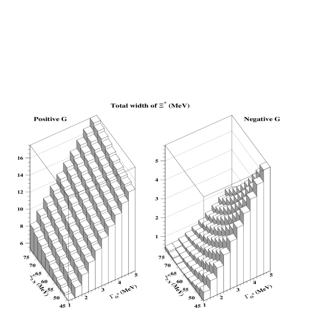
Figure 2: The total width of $\Xi_{\overline{10}}$ as a function of $\Gamma_{\Theta^{+}}$ and $\Sigma_{\pi\,N}$. The two plots correspond to the positive and negative solutions for $G_{\overline{10}}$.

III.3 Decays of $N_{\overline{10}}$

Next we turn to the decays of $N_{\overline{10}}$. An examination shows that the total width of $N_{\overline{10}}$ only weakly depends on $\Gamma_{\Theta^{+}}$ and $G_{\overline{10}}$ and that the dependence on $\Sigma_{\pi\,N}$ is more important because the $\theta_{1}$ mixing angle crucially depends on $\Sigma_{\pi\,N}$, see Eq. (15). As an example of this trend, in Fig. 3 we present $\Gamma_{N_{\overline{10}}}$ as a function of the $\theta_{2}$ and $\theta_{3}$ mixing angles for $\Gamma_{\Theta^{+}}=1$ MeV (upper row) and 5 MeV (lower row) and for $\Sigma_{\pi\,N}=45$ and 75 MeV. All plots correspond to the positive $G_{\overline{10}}$ solution. One sees from Fig. 3 that the total width of $N_{\overline{10}}$ depends very dramatically on all mixing angles and, in general, can be very large.

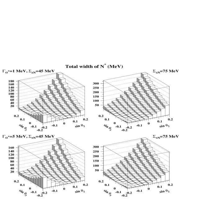
Figure 3: The total width of $N_{\overline{10}}$ as a function of $\theta_{2}$ and $\theta_{3}$ at $\Gamma_{\Theta^{+}}=1$ and 5 MeV and $\Sigma_{\pi\,N}=45$ and 75 MeV.

It is instructive to separately examine different $N_{\overline{10}}$ partial decay widths. As an example of such an analysis, we plot $\Gamma_{N_{\overline{10}}\to N\,\pi}$, $\Gamma_{N_{\overline{10}}\to N\,\eta}$, $\Gamma_{N_{\overline{10}}\to\Lambda\,K}$ and $\Gamma_{N_{\overline{10}}\to\Delta\,\pi}$ at $\Gamma_{\Theta^{+}}=1$ and 5 MeV and $\Sigma_{\pi\,N}=45$ and 75 MeV as functions of $\theta_{2}$ and $\theta_{3}$ in Figs. 4 and 5. Again, we present the results with the positive $G_{\overline{10}}$ solution because the results with the negative $G_{\overline{10}}$ solution give too large $\Gamma_{N_{\overline{10}}\to N\,\pi}$ which seems to be ruled out by the PWA of Arndt2004 . Note that the $N_{\overline{10}}\to\Sigma\,K$ decay is kinematically impossible for the used $N_{\overline{10}}$ mass.

Figures 4 and 5 reveal the following approximate correlation between the partial decays widths. Small $\Gamma_{N_{\overline{10}}\to N\,\pi}$ is correlated with small $\Gamma_{N_{\overline{10}}\to\Lambda\,K}$ and $\Gamma_{N_{\overline{10}}\to\Delta\,\pi}$. At the same time, $\Gamma_{N_{\overline{10}}\to N\,\eta}$ does not have to be small. The $\Gamma_{N_{\overline{10}}\to\Delta\,\pi}$ peaks at large positive values of the mixing angles because the decay is possible only due to the mixing. The variation of $\Gamma_{\Theta^{+}}$ or $\Sigma_{\pi\,N}$ in the considered ranges does not significantly change this trend (except for $\Gamma_{N_{\overline{10}}\to N\,\pi}$ at $\Gamma_{\Theta^{+}}=5$ MeV and $\Sigma_{\pi\,N}=45$ MeV and for $\Gamma_{N_{\overline{10}}\to\Delta\,\pi}$ at $\Sigma_{\pi\,N}=45$ MeV in the region $\sin\theta_{2,3}\approx-0.2$) but merely affects the absolute values of the partial decay widths.

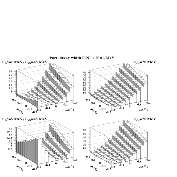
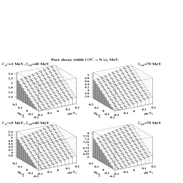
Figure 4: $\Gamma_{N_{\overline{10}}\to N\,\pi}$ and $\Gamma_{N_{\overline{10}}\to N\,\eta}$ as functions of $\theta_{2}$ and $\theta_{3}$ for $\Gamma_{\Theta^{+}}=1$ and 5 MeV and $\Sigma_{\pi\,N}=45$ and 75 MeV.

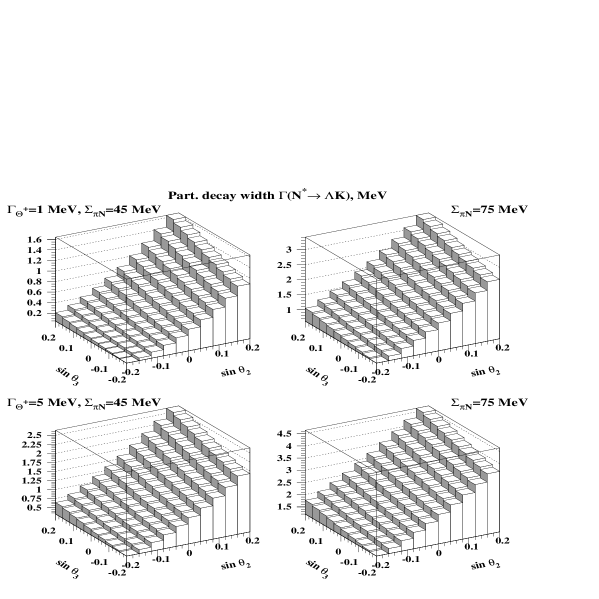
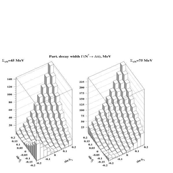
Figure 5: $\Gamma_{N_{\overline{10}}\to\Lambda\,K}$ and $\Gamma_{N_{\overline{10}}\to\Delta\,\pi}$ as functions of $\theta_{2}$ and $\theta_{3}$ for $\Gamma_{\Theta^{+}}=1$ and 5 MeV and $\Sigma_{\pi\,N}=45$ and 75 MeV. $\Gamma_{N_{\overline{10}}\to\Delta\,\pi}$ does not depend on $\Gamma_{\Theta^{+}}$.

The trend of the correlation among the partial decay widths of $N_{\overline{10}}$ presented in Figs. 4 and 5 seems to be in a broad agreement with the present experimental situation. First, the PWA analysis of Arndt2004 indicates that the candidate $N_{\overline{10}}$ state with mass near 1680 MeV should have a small partial decay width for the decay into the $N\,\pi$ final state, $\Gamma_{N_{\overline{10}}\to N\,\pi}\leq 0.5$ MeV. We find that such small $\Gamma(N_{\overline{10}}\to N\,\pi)$ solutions do exist (see the following discussion). Second, the GRAAL experiment indicates the existence of a narrow nucleon resonance near 1670 MeV in the reaction $\gamma\,n\to n\,\eta$ GRAAL2 . Therefore, $\Gamma_{N_{\overline{10}}\to N\,\eta}$ should not be too small. Third, the STAR collaboration observes a narrow peak at $1734\pm 0.5\pm 5$ MeV and only a weak indication of a narrow peak at $1693\pm 0.5$ MeV in the $\Lambda\,K_{S}$ invariant mass STAR . The former peak is interpreted as a candidate for $N_{\overline{10}}$; the latter is hypothesized to be a candidate for the $\Xi(1690)$ state. This does not fit well our picture of the $N_{\overline{10}}$ decays. Therefore, until the STAR results and conclusions are proven by other groups, in the present analysis we ignore the peak at $1734$ MeV and assume that the peak at $1693$ MeV corresponds to the $N_{\overline{10}}$. In this case, we interpret the STAR results as an indication that the $\Gamma_{N_{\overline{10}}\to\Lambda\,K}$ is not larger than 1-2 MeV, i.e. the decay is possibly suppressed.

An examination of the general expressions for the $N_{\overline{10}}$ decay widths in Eq. (10) shows that the picture of the $N_{\overline{10}}$ decays, which emerges from the present experimental information, can be qualitatively justified. Indeed, because of the minus sign in front of the positive $G_{\overline{10}}$ and $G_{8}$ coupling constants and negative values of $g_{N_{i}N\,\eta}$ in the expression for $g_{N_{\overline{10}}N\,\eta}$, the $g_{N_{\overline{10}}N\,\eta}$ coupling constant can be enhanced compared to the $g_{N_{\overline{10}}N\,\pi}$ coupling constant where the terms proportional to $G_{8}$ and $g_{N_{i}N\,\pi}$ partially cancel the $G_{\overline{10}}$ contribution. Note that this logic works only if $G_{\overline{10}}$ is positive. Therefore, unless specified, we always give our predictions for the positive $G_{\overline{10}}$, see Fig. 1. As to the $N_{\overline{10}}\to\Lambda\,K$ decay, its partial width is suppressed in any case by the phase space factor.

In order to quantitatively examine how well the above mentioned constraints on the partial decay widths of $N_{\overline{10}}$ are satisfied and at which mixing angles, in Figs. 7 and 8 we show the partial decay widths of Figs. 4 and 5 only at those $\theta_{2}$ and $\theta_{3}$ which correspond to $\Gamma_{N_{\overline{10}}\to N\,\pi}\leq 1$ MeV. If this criterion is not met, the partial decay widths are not shown (they are formally set to zero).

Figure 6 presents the allowed regions of $\sin\theta_{2,3}$ when the $\Gamma_{N_{\overline{10}}\to N\,\pi}\leq 1$ MeV condition is imposed. At given $\sin\theta_{2}$, the two solid curves present the maximal and minimal values of $\sin\theta_{3}$.

Figure 6: The regions of the $\theta_{2}$ and $\theta_{2}$ mixing angles allowed by the $\Gamma_{N_{\overline{10}}\to N\,\pi}\leq 1$ MeV condition.

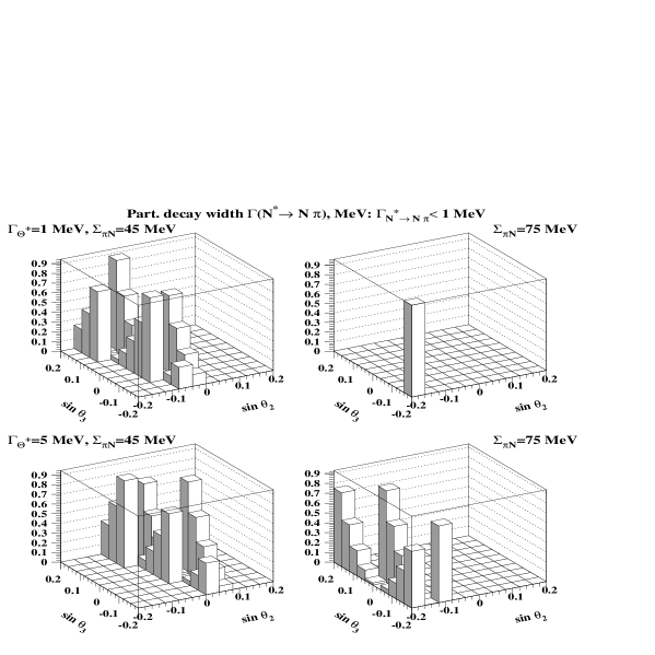
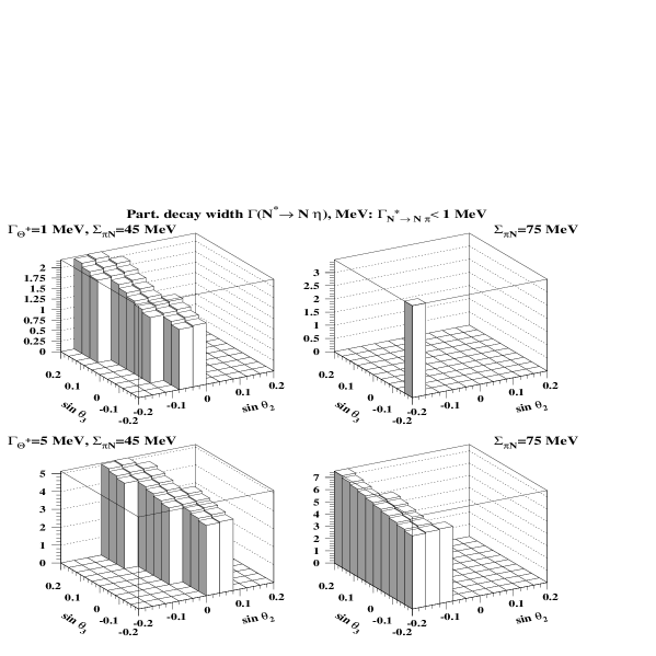
Figure 7: $\Gamma_{N_{\overline{10}}\to N\,\pi}$ and $\Gamma_{N_{\overline{10}}\to N\,\eta}$ as functions of $\theta_{2}$ and $\theta_{3}$. The decay widths are shown only where $\Gamma_{N_{\overline{10}}\to N\,\pi}\leq 1$ MeV.

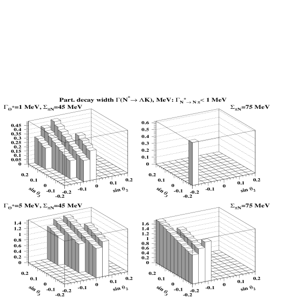
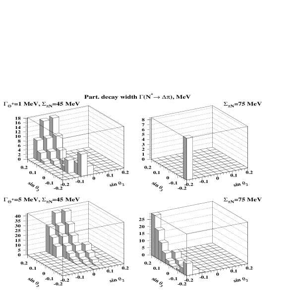
Figure 8: $\Gamma_{N_{\overline{10}}\to\Lambda\,K}$ and $\Gamma_{N_{\overline{10}}\to\Delta\,\pi}$ as functions of $\theta_{2}$ and $\theta_{3}$. The decay widths are shown only where $\Gamma_{N_{\overline{10}}\to N\,\pi}\leq 1$ MeV.

As seen from Figs. 7 and 8, an appropriate choice of the $\theta_{2}$ and $\theta_{3}$ mixing angles allows to simultaneously suppress the $\Gamma_{N_{\overline{10}}\to N\,\pi}$ and $\Gamma_{N_{\overline{10}}\to\Lambda\,K}$ (the latter is much more significantly suppressed at small values of the total width of $\Theta^{+}$) decay widths and to have the unsuppressed $\Gamma_{N_{\overline{10}}\to N\,\eta}$ partial decay widths – in accord with the present experimental situation with the $N_{\overline{10}}$ decays, if $N_{\overline{10}}$ is identified with the GRAAL’s $N(1670)$.

In addition, imposing the $\Gamma_{N_{\overline{10}}\to N\,\pi}\leq 1$ MeV constraint, we find that the sum of the considered two-body partial decay widths of $N_{\overline{10}}$, $\Gamma_{N_{\overline{10}}}^{{\rm 2-body}}$, varies in the interval summarized in Table 1. Note that our analysis predicts the $N_{\overline{10}}$ total width which is somewhat larger than predicted by the PWA of Arndt2004 .

$\Gamma_{\Theta^{+}}$ (MeV)	$\Sigma_{\pi\,N}$ (MeV)	$\Gamma_{N_{\overline{10}}}^{{\rm 2-body,min}}$ (MeV)	$\Gamma_{N_{\overline{10}}}^{{\rm 2-body,max}}$ (MeV)
1	45	2.1	30
1	75	8.2	18
5	45	5.2	66
5	75	7.8	44

Table 1: The range of change of $\Gamma_{N_{\overline{10}}}^{{\rm 2-body}}$.

Note that because of the approximate correlation between $\Gamma_{N_{\overline{10}}\to N\,\pi}$ and $\Gamma_{N_{\overline{10}}\to\Lambda\,K}$ in our analysis, it seems unnatural to simultaneously have sizable $\Gamma_{N_{\overline{10}}\to\Lambda\,K}$ and suppressed $\Gamma_{N_{\overline{10}}\to N\,\pi}$. Therefore, our analysis disfavors the identification of the peak at 1734 MeV seen by the STAR collaboration in the $\Lambda\,K_{S}$ invariant mass STAR with $N_{\overline{10}}$, which should have a suppressed partial decay width for the $N\,\pi$ final state Arndt2004 .

III.4 Decays of $\Sigma_{\overline{10}}$

Next we turn to the decays of $\Sigma_{\overline{10}}$ which we consider analogously to the decays of $N_{\overline{10}}$. Figure 9 depicts the dependence of the total width of the $\Sigma_{\overline{10}}$, $\Gamma_{\Sigma_{\overline{10}}}$, on the $\theta_{2}$ and $\theta_{3}$ mixing angles and on $\Gamma_{\Theta^{+}}$ and $\Sigma_{\pi\,N}$. Unlike the total width of $N_{\overline{10}}$, $\Gamma_{\Sigma_{\overline{10}}}$ depends on both $\Gamma_{\Theta^{+}}$ and $\Sigma_{\pi\,N}$.

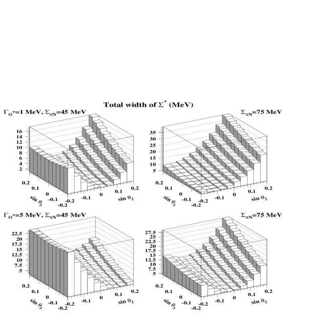
Figure 9: The total width of $\Sigma_{\overline{10}}$ as a function of $\theta_{2}$ and $\theta_{3}$ for $\Gamma_{\Theta^{+}}=1$ and 5 MeV and for $\Sigma_{\pi\,N}=45$ and 75 MeV.

Next we examine correlations between partial decay widths of $\Sigma_{\overline{10}}$. In Figs. 10 and 11 we present $\Gamma_{\Sigma_{\overline{10}}\to\Lambda\,\pi}$, $\Gamma_{\Sigma_{\overline{10}}\to\Sigma\,\pi}$, $\Gamma_{\Sigma_{\overline{10}}\to N\,\overline{K}}$ and $\Gamma_{\Sigma_{\overline{10}}\to\Sigma_{10}\,\pi}$ partial decay widths as functions of $\theta_{2}$ and $\theta_{3}$ for $\Gamma_{\Theta^{+}}=1$ and 5 MeV and for $\Sigma_{\pi\,N}=45$ and 75 MeV. The $\Gamma_{\Sigma_{\overline{10}}\to\Sigma\,\eta}$ partial decay width is very small because the decay takes place very near its threshold – we do not show $\Gamma_{\Sigma_{\overline{10}}\to\Sigma\,\eta}$ in this work.

The approximate correlation between the partial decay widths, which is seen in the $N_{\overline{10}}$ case, is much less pronounced in the case of $\Sigma_{\overline{10}}$. The following, very approximate, trend can be seen in Figs. 10 and 11: At $\sin\theta_{2}\approx-0.2$, large $\Gamma_{\Sigma_{\overline{10}}\to\Lambda\,\pi}$ correspond to large $\Gamma_{\Sigma_{\overline{10}}\to N\,\overline{K}}$ and to the suppressed $\Gamma_{\Sigma_{\overline{10}}\to\Sigma\,\pi}$ (except for $\Gamma_{\Theta^{+}}=5$ MeV and $\Sigma_{\pi\,N}=45$ MeV); suppressed $\Gamma_{\Sigma_{\overline{10}}\to\Lambda\,\pi}$ correspond to suppressed $\Gamma_{\Sigma_{\overline{10}}\to N\,\overline{K}}$ ($\Gamma_{\Sigma_{\overline{10}}\to\Lambda\,\pi}$ at $\Gamma_{\Theta^{+}}=1$ MeV and $\Sigma_{\pi\,N}=75$ MeV is an exception); $\Gamma_{\Sigma_{\overline{10}}\to\Sigma(1385)\,\pi}$ increases towards large and positive $\theta_{2}$ and $\theta_{3}$ mixing angles.

These trends can be traced back to the general expressions for the $\Sigma_{\overline{10}}$ coupling constants, see Eq. (11), along with the octet coupling constants of Eq. (17). For instance, at $\Gamma_{\Theta^{+}}=1$ MeV, the increase of $\theta_{2}$ towards its maximal value (as seen from Eq. (17), mixing with octet 4 hardly matters for the $\Sigma_{\overline{10}}$ decays) leads to an increase of $g_{\Sigma_{\overline{10}}\to\Lambda\,\pi}$ and $g_{\Sigma_{\overline{10}}\to\Sigma\,\pi}$ and to a decrease of $g_{\Sigma_{\overline{10}}\to N\,\overline{K}}$.

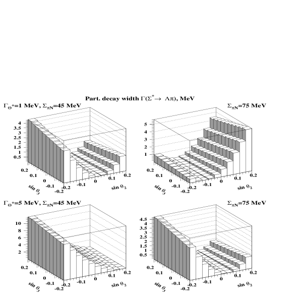
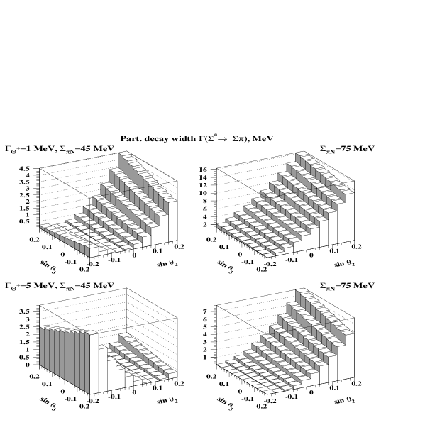
Figure 10: $\Gamma_{\Sigma_{\overline{10}}\to\Lambda\,\pi}$ and $\Gamma_{\Sigma_{\overline{10}}\to\Sigma\,\pi}$ as functions of $\theta_{2}$ and $\theta_{3}$ for $\Gamma_{\Theta^{+}}=1$ MeV and 5 and $\Sigma_{\pi\,N}=45$ and 75 MeV.

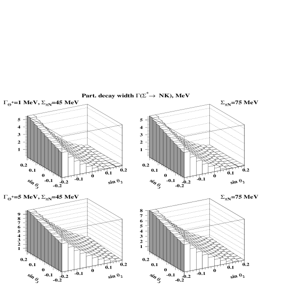
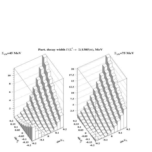
Figure 11: $\Gamma_{\Sigma_{\overline{10}}\to N\,K}$ and $\Gamma_{\Sigma_{\overline{10}}\to\Sigma(1385)\,\pi}$ as functions of $\theta_{2}$ and $\theta_{3}$ for $\Gamma_{\Theta^{+}}=1$ and 5 MeV and $\Sigma_{\pi\,N}=45$ and 75 MeV. $\Gamma_{\Sigma_{\overline{10}}\to\Sigma(1385)\,\pi}$ does not depend on $\Gamma_{\Theta^{+}}$.

Finally, in Figs. 12 and 13 we show the partial decay widths of $\Sigma_{\overline{10}}$ in the range of $\theta_{2}$ and $\theta_{3}$ where $\Gamma_{N_{\overline{10}}\to N\,\pi}\leq 1$ MeV.

Taking the sum of the considered two-body partial decay widths of $\Sigma_{\overline{10}}$, $\Gamma_{\Sigma_{\overline{10}}}^{{\rm 2-body}}$, we find that in presence of the $\Gamma_{N_{\overline{10}}\to N\,\pi}\leq 1$ MeV constraint, $\Gamma_{\Sigma_{\overline{10}}}^{{\rm 2-body}}$ varies in the interval summarized in Table 2.

$\Gamma_{\Theta^{+}}$ (MeV)	$\Sigma_{\pi\,N}$ (MeV)	$\Gamma_{\Sigma_{\overline{10}}}^{{\rm 2-body,min}}$ (MeV)	$\Gamma_{N_{\overline{10}}}^{{\rm 2-body,max}}$ (MeV)
1	45	0.95	9.1
1	75	5.7	6.5
5	45	2.9	15
5	75	5.3	15

Table 2: The range of change of $\Gamma_{\Sigma_{\overline{10}}}^{{\rm 2-body}}$.

In the spirit of the antidecuplet, $\Sigma_{\overline{10}}$ appears to be much narrower than any known $\Sigma$ baryon with mass larger than 1650 MeV PDG .

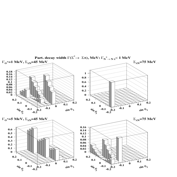
Figure 12: $\Gamma_{\Sigma_{\overline{10}}\to\Lambda\,\pi}$ and $\Gamma_{\Sigma_{\overline{10}}\to\Sigma\,\pi}$ as functions of $\theta_{2}$ and $\theta_{3}$. The decay widths are shown only where $\Gamma_{N_{\overline{10}}\to N\,\pi}\leq 1$ MeV.

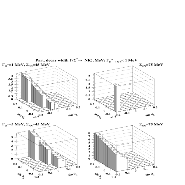
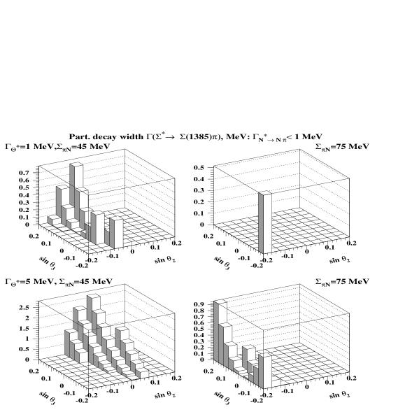
Figure 13: $\Gamma_{\Sigma_{\overline{10}}\to N\,\overline{K}}$ and $\Gamma_{\Sigma_{\overline{10}}\to\Sigma(1385)\,\pi}$ as functions of $\theta_{2}$ and $\theta_{3}$. The decay widths are shown only where $\Gamma_{N_{\overline{10}}\to N\,\pi}\leq 1$ MeV.

Among the experiments reporting the $\Theta^{+}$ signal, there were four experiments Neutrino ; SVD ; HERMES ; ZEUS where the $\Theta^{+}$ was observed as a peak in the $p\,K_{S}$ invariant mass and strangeness was not tagged. Since $\Sigma_{\overline{10}}$ decays in the same final state ($N\,\overline{K}$), the four experiments give direct information on the $\Sigma_{\overline{10}}\to N\,\overline{K}$ decay – virtually the only experimental piece of information on $\Sigma_{\overline{10}}$! Below we shall consider the relevant results of the four experiments in some detail.

The analysis of neutrino-nuclear (mostly neon) interaction data Neutrino clearly reveals the $\Theta^{+}$ peak as well as a number of other peaks in the $1650<M_{p\,K_{S}}<1850$ MeV mass region, which cannot be suppressed by the random-star elimination procedure, see Fig. 3 of Neutrino . This is an agreement with the present analysis (Figs. 11 and 13), which shows that the branching ratio for the $\Sigma_{\overline{10}}\to N\,\overline{K}$ decay width is essential. Obviously, any of the peaks of Neutrino in the 1700-1800 MeV mass range could be a good candidate for $\Sigma_{\overline{10}}$.

Similar conclusions apply to the SVD collaboration result SVD . Before the cuts aimed to enhance the $\Theta^{+}$ signal are imposed, the $p\,K_{S}$ invariant mass spectrum contains at least two prominent peaks in the 1700-1800 MeV mass range (see Fig. 5 of SVD ), each of which can be interpreted as $\Sigma_{\overline{10}}$.

The HERMES HERMES and ZEUS ZEUS $p\,K_{S}$ invariant mass spectra extend only up to 1.7 MeV and, therefore, do not allow to make any conclusions about the $\Sigma_{\overline{10}}$.

In addition to the $p\,K_{S}$ invariant mass spectrum, the HERMES collaboration also presents the $\Lambda\,\pi$ invariant mass spectrum in order to see if the observed peak in the $p\,K_{S}$ final state is indeed generated by the $\Theta^{+}$ and not by some yet unknown $\Sigma^{\ast}$ resonance Lorenzon . The $\Lambda\,\pi$ invariant mass spectrum has no resonance structures except for the prominent $\Sigma(1385)$ peak. According to our analysis, the $\Gamma_{\Sigma_{\overline{10}}\to\Lambda\,\pi}$ partial decay width is in general not large. Moreover, at a small total width of the $\Theta^{+}$ and large $\Sigma_{\pi\,N}$, $\Gamma_{\Sigma_{\overline{10}}\to\Lambda\,\pi}$ is dramatically suppressed which seems to be exactly what is needed to comply with no-observation of $\Sigma_{\overline{10}}$ in the HERMES $\Lambda\,\pi$ invariant mass spectrum!

However, it is difficult to make any quantitative conclusions from the HERMES spectrum because of its course scale. Indeed, if one naively assumes that the HERMES spectrum reveals only the well-known $\Sigma(1385)$, several well-established $\Sigma$ baryons PDG with noticeable branching ratios to the $\Lambda\,\pi$ final state are missed.

In our opinion, the Neutrino ; SVD data already contain an indication for a narrow $\Sigma_{\overline{10}}$ member of the antidecuplet in the 1700-1800 MeV mass range and the HERMES ; ZEUS ; Lorenzon data do not rule out its existence. Obviously, a dedicated search for the $\Sigma_{\overline{10}}$ signal in the $p\,K_{S}$ and $\Lambda\,\pi$ invariant mass spectra is needed in order to address several key issues surrounding this least known member of the antidecuplet.

It is interesting that one can offer a candidate $\Sigma_{\overline{10}}$ state, $\Sigma(1770)$, which has been known for almost three decades PDG ; Gopal77 . Indeed, the one-star $\Sigma(1770)$ has the required $J^{P}=1/2^{+}$ and the mass, a $14\pm 4$ % branching ratio in the $N\,\overline{K}$ final state and poorly known but still probably rather small branching ratios into the $\Lambda\,\pi$ and $\Sigma\,\pi$ final states. Moreover, our comprehensive SU(3) analysis of baryon multiplets GPreview disfavors that $\Sigma(1770)$ belongs to any octet or decuplet, i.e. it is very natural to assign $\Sigma(1770)$ to the antidecuplet, see also Hosaka .

However, the $\Sigma(1770)$ with the total width $72\pm 10$ MeV appears to be too wide for the antidecuplet, see Table 2. On the other hand, taking the $\Sigma(1770)$ branching ratios at their face values Gopal77 ,

$$Br(N\,\overline{K})=0.14\pm 0.04$$

$$\sqrt{Br(N\,\overline{K})Br(\Lambda\,\pi)}<0.04$$

$$\sqrt{Br(N\,\overline{K})Br(\Sigma\,\pi)}<0.04\,,$$ (18)

we observe that the experimental value for the sum of the two-hadron branching ratios is less than 20%, i.e. the two-hadron decays constitute less than 1/5 of all possible (including many-body) decays. This indicates that our predictions for the $\Gamma_{\Sigma_{\overline{10}}}^{{\rm 2-body}}$, which is of the order of $7-15$ MeV, do not exclude the $\Sigma(1770)$ as candidate for $\Sigma_{\overline{10}}$.

In conclusion, our qualitatively reasonable description of the decays of the $\Sigma(1770)$ along with its “correct” spin, parity and mass makes $\Sigma(1770)$ an appealing candidate for $\Sigma_{\overline{10}}$. This conjecture can be tested only by a dedicated analysis of the $\Sigma$ baryon spectrum in the 1700-1800 mass range.

It was argued in 27plet that the antidecuplet mixing with 27-plet and 35-plet SU(3) representations has a significant impact on the antidecuplet decays. Therefore, in order to study how robust our predictions for the antidecuplet decays with respect to the additional mixing, in Appendix B we explicitly add the 27-plet and 35-plet contributions to the antidecuplet coupling constants and repeat the entire analysis of Sect. III. We arrive at the following two scenarios corresponding to two possible solutions for the $G_{\overline{10}}$ coupling constant.

When we use the larger and always positive $G_{\overline{10}}$ solution, imposing the $\Gamma_{N_{\overline{10}}\to N\,\pi}<1$ MeV condition, we reproduce the qualitative picture of the $N_{\overline{10}}$ decays presented in Sect. III. At the same time, the correlation between the $\Sigma_{\overline{10}}$ change. For instance, we generally have $\Gamma_{\Sigma_{\overline{10}}\to\Lambda\,\pi}>\Gamma_{\Sigma_{\overline{10}}\to N\,\overline{K}}$, which makes it impossible to identify $\Sigma_{\overline{10}}$ with $\Sigma(1770)$.

Using the other solution for $G_{\overline{10}}$, which is mostly negative and becomes positive and small in magnitude towards larger $\Sigma_{\pi\,N}$, we can obtain a picture of the $N_{\overline{10}}$ decays, which is marginally compatible with the one presented in Sect. III, only if $\Gamma_{\Theta^{+}}=1$ MeV and $\Sigma_{\pi\,N}=75$ MeV. At the same time, the correlation between the partial decay widths of $\Sigma_{\overline{10}}$ reminds the pattern of the $\Sigma(1770)$ decays. A characteristic feature of this scenario of the antidecuplet decays is rather narrow $N_{\overline{10}}$ and $\Sigma_{\overline{10}}$.

IV Conclusions and Discussion

In this work, we consider mixing of the antidecuplet with three $J^{P}=1/2^{+}$ octets in the framework of approximate flavor SU(3) symmetry. These are the ground-state octet, the octet containing $N(1440)$, $\Lambda(1600)$, $\Sigma(1660)$ and $\Xi(1690)$ (referred to as octet 3) and the octet containing $N(1710)$, $\Lambda(1800)$, $\Sigma(1880)$ and $\Xi(1950)$ (referred to as octet 4). Assuming that SU(3) symmetry is broken only by non-equal masses of hadrons within a given unitary multiplet and by small mixing among multiplets and that SU(3) symmetry is exact in the decay vertices, we derived expressions for the partial decay widths all members of the antidecuplet in the limit of small mixing angles. The results are expressed in terms of the universal SU(3) coupling constants and three mixing angles $\theta_{i}$. For the transition between the antidecuplet and the ground-state octet, the coupling constants and the $\theta_{1}$ mixing angle are determined by the chiral quark soliton model. For the transition between the antidecuplet and octets 3 and 4, the coupling constants are determined by fitting to the octet decays, while the $\theta_{2}$ and $\theta_{3}$ mixing angles are left as free parameters. Finally, the total width of the $\Theta^{+}$ and the pion-nucleon sigma term are treated as external parameters which are varied in the following intervals: $1\leq\Gamma_{\Theta^{+}}\leq 5$ MeV; $45\leq\Sigma_{\pi\,N}\leq 75$ MeV. The $\theta_{2}$ and $\theta_{3}$ mixing angles are varied in the $-0.2\leq\sin\theta_{2,3}\leq 0.2$ interval.

In this analysis, the $\theta_{2}$ and $\theta_{3}$ mixing angles were constrained by identifying the $N_{\overline{10}}$ state with the peak around 1670 MeV observed by the GRAAL experiment in the $\gamma\,n\to n\,\eta$ reaction GRAAL2 . The fact that $N_{\overline{10}}$ might have mass around 1670 was earlier predicted in DP2004 ; Arndt2004 . In general, the nowadays experimental information on the $N_{\overline{10}}$ decays can be qualitatively summarized as follows: $\Gamma_{N_{\overline{10}}\to N\,\eta}$ is sizable GRAAL2 ; $\Gamma_{N_{\overline{10}}\to N\,\pi}$ is small Arndt2004 ; $\Gamma_{N_{\overline{10}}\to\Lambda\,K}$ is possibly suppressed in order to comply with the STAR result STAR ; the total width of $N_{\overline{10}}$ is of the order of 10-20 MeV Arndt2004 . We find that all these conditions can be met by a suitable choice of $\theta_{2}$ and $\theta_{3}$, see Figs. 6, 7 and 8.

Our approach based on the mixing of the antidecuplet with three octets appears to be an improvement over the scenario of Arndt2004 , which implied that the antidecuplet mixes only with the ground-state octet, because we are able to demonstrate that a narrow $\Theta^{+}$ and small $\Gamma_{N_{\overline{10}}\to N\,\pi}$ become consistent due to the mixing with several multiplet (this was only hypothesized in Arndt2004 ).

After the mixing angles are constrained by the $N_{\overline{10}}$ decays, we make definite predictions for the $\Sigma_{\overline{10}}$ decays, see Figs. 12 and 13. In particular, at $\Gamma_{\Theta^{+}}=1$ MeV and $\Sigma_{\pi\,N}=75$ MeV, we predict that $\Gamma_{\Sigma_{\overline{10}}\to N\,\overline{K}}$ is significantly enhanced compared to $\Gamma_{\Sigma_{\overline{10}}\to\Lambda\,\pi}$ and $\Gamma_{\Sigma_{\overline{10}}\to\Sigma\,\pi}$. This correctly reproduces the trend of the branching ratios of $\Sigma(1770)$, a known one-star $\Sigma$ baryon with $J^{P}=1/2^{+}$ PDG . However, the sum of the predicted two-body partial decay widths is much smaller than the experimental value for the total width of $\Sigma(1770)$, $\Gamma_{\Sigma(1770)}=72\pm 10$ MeV. In any case, we believe that our conjecture that $\Sigma_{\overline{10}}$ could be identified with $\Sigma(1770)$ deserves further experimental and phenomenological analyses.

We discuss that a narrow $\Sigma_{\overline{10}}$ state with mass near 1770 MeV could be searched for in the $K_{S}\,p$ invariant mass spectrum using the available data which already revealed the $\Theta^{+}$ signal Neutrino ; SVD .

In order to access a possible theoretical uncertainty of our predictions, we examine how our predictions for the antidecuplet decays change when we introduce an additional mixing of the antidecuplet with a 27-plet 27plet . We observe the following two scenarios, which correspond to two possible solutions for the $G_{\overline{10}}$ coupling constant. Using the larger $G_{\overline{10}}$ solution and imposing the $\Gamma_{N_{\overline{10}}\to N\,\pi}$ constraint, we reproduce the qualitative picture of the $N_{\overline{10}}$ decays presented in Sect. III. At the same time, the correlation between the $\Sigma_{\overline{10}}$ change, which makes it impossible to identify $\Sigma_{\overline{10}}$ with $\Sigma(1770)$.

Using the smaller $G_{\overline{10}}$ solution, which is mostly negative and becomes positive at small $\Gamma_{\Theta^{+}}$ and large $\Sigma_{\pi\,N}$, we can still obtain a picture of the $N_{\overline{10}}$ decays, which is marginally compatible with the one presented in Sect. III. At the same time, the correlation between the partial decay widths of $\Sigma_{\overline{10}}$ is similar to that of $\Sigma(1770)$. In addition, this scenario predicts rather narrow $N_{\overline{10}}$ and $\Sigma_{\overline{10}}$ states.

Any further progress in our understanding of the properties of the antidecuplet should come from experiments. One of the main purposes of this work was to show that it is possible to bring order to a multitude of direct and indirect experimental information on the antidecuplet decays using the very fundamental and successful principle of approximate flavor SU(3) symmetry and to ignite interest among experimentalists in studying all members of the antidecuplet.

Appendix A Determination of SU(3) coupling constants of octets 3 and 4

In this appendix, we derive the SU(3) coupling constants of octets 3 and 4, which are summarized in Eq. (17. Octet 3 consists of $N(1440)$, $\Lambda(1600)$, $\Sigma(1660)$ and $\Xi(1690)$; octet 4 consists of $N(1710)$, $\Lambda(1810)$, $\Sigma(1880)$ and $\Xi(1950)$.

In general, the SU(3) coupling constants of a given unitary multiplet can be determined by performing a $\chi^{2}$ fit to the experimentally measured partial decay widths, see e.g. Samios74 ; GPreview . In some cases, the fit is unsuccessful, which indicates that the considered multiplet is most likely mixed with some other multiplet(s). Our analysis shows that while approximate flavor SU(3) symmetry can account for the known decays of octet 4, SU(3) fails for octet 4 because SU(3) incorrectly predicts the sign of the $\Sigma(1880)\to\Sigma\,\pi$ amplitude. A possible solution, which remedies the problem, is to introduce a mixing between octets 3 and 4.

The mixing of two octets can be parameterized in terms of four mixing angles: $\Theta_{N}$, $\Theta_{\Lambda}$, $\Theta_{\Sigma}$ and $\Theta_{\Xi}$. However, only two mixing angles are independent. In our analysis, we take $\Theta_{N}$ and $\Theta_{\Sigma}$ as the independent mixing angles. Then, the physical decay coupling constants of octet 3 and 4, which we generically call $G_{2}$ and $G_{3}$, are expressed in terms of the unmixed coupling constants, $G_{2}^{0}$ and $G_{3}^{0}$, and the mixing angle $\theta$

$$G_{2}=\cos\theta\,G_{2}^{0}+\sin\theta\,G_{3}^{0}$$

$$G_{3}=-\sin\theta\,G_{2}^{0}+\cos\theta\,G_{3}^{0}\,.$$ (19)

In particular, the SU(3) coupling constants of $N(1440)$ from octet 3, which are proportional to the relevant coupling constants entering Eq. (10), have the following form

$$G_{N_{2}N\,\pi}=\frac{1}{2\sqrt{5}}g_{N_{2}N\,\pi}=\frac{9}{20}\left(G_{8}^{(2)}(1+\alpha^{(2)})\cos\phi_{N}+G_{8}^{(3)}(1+\alpha^{(3)})\sin\phi_{N}\right)$$

$$G_{N_{2}N\,\eta}=\frac{1}{2\sqrt{5}}g_{N_{2}N\,\eta}=-\frac{3}{20}\left(G_{8}^{(2)}(1-3\,\alpha^{(2)})\cos\phi_{N}+G_{8}^{(3)}(1-3\,\alpha^{(3)})\sin\phi_{N}\right)$$

$$G_{N_{2}\Lambda\,K}=\frac{1}{2\sqrt{5}}g_{N_{2}\Lambda\,K}=-\frac{3}{20}\left(G_{8}^{(2)}(1+3\,\alpha^{(2)})\cos\phi_{N}+G_{8}^{(3)}(1+3\,\alpha^{(3)})\sin\phi_{N}\right)$$

$$G_{N_{2}\Delta\,\pi}=\frac{2}{\sqrt{5}}g_{N_{2}\Delta\,\pi}=-\frac{2}{\sqrt{5}}\left(G_{10}^{(2)}\cos\phi_{N}+G_{10}^{(3)}\sin\phi_{N}\right)\,.$$ (20)

For the $N(1710)$ from octet 4, the relevant $g_{N_{3}}$ coupling constants are obtained from Eq. (20) after the replacement $\cos\phi_{N}\to-\sin\phi_{N}$ and $\sin\phi_{N}\to\cos\phi_{N}$.

The parameters $G_{8}^{(2,3)}$, $\alpha^{(2,3)}$ and $G_{10}^{(2,3)}$ and the mixing angles $\theta_{N,\Sigma}$ are determined from the $\chi^{2}$ fit to the combined set of experimentally measured partial decay widths of octets 3 and 4.

The SU(3) coupling constants of $\Sigma(1660)$, which enter Eq. (11), have the following structure

$$G_{\Sigma_{2}\Lambda\,\pi}=\frac{1}{2\sqrt{5}}g_{\Sigma_{2}\Lambda\,\pi}=\frac{3}{10}\left(G_{8}^{(2)}\cos\phi_{\Sigma}+G_{8}^{(3)}\sin\phi_{\Sigma}\right)$$

$$G_{\Sigma_{2}\Sigma\,\eta}=\frac{1}{2\sqrt{5}}g_{\Sigma_{2}\Sigma\,\eta}=\frac{3}{10}\left(G_{8}^{(2)}\cos\phi_{\Sigma}+G_{8}^{(3)}\sin\phi_{\Sigma}\right)$$

$$G_{\Sigma_{2}\Sigma\,\pi}=\frac{1}{\sqrt{30}}g_{\Sigma_{2}\Sigma\,\pi}=\frac{3\sqrt{6}}{10}\left(G_{8}^{(2)}\,\alpha^{(2)}\cos\phi_{\Sigma}+G_{8}^{(3)}\,\alpha^{(3)}\sin\phi_{\Sigma}\right)$$

$$G_{\Sigma_{2}N\,\overline{K}}=\frac{1}{\sqrt{30}}g_{\Sigma_{2}N\,\overline{K}}=-\frac{3\sqrt{3}}{10\sqrt{2}}\left(G_{8}^{(2)}(1-\alpha^{(2)})\cos\phi_{\Sigma}+G_{8}^{(3)}(1-\alpha^{(3)})\sin\phi_{\Sigma}\right)$$

$$G_{\Sigma_{2}\Sigma_{10}\,\pi}=\frac{\sqrt{30}}{15}g_{\Sigma_{2}\Sigma_{10}\,\pi}=-\frac{\sqrt{30}}{15}\left(G_{10}^{(2)}\cos\phi_{\Sigma}+G_{10}^{(3)}\sin\phi_{\Sigma}\right)\,.$$ (21)

The corresponding $\Sigma(1880)$ coupling constants are obtained from Eq. (21) after the replacement $\cos\phi_{\Sigma}\to-\sin\phi_{\Sigma}$ and $\sin\phi_{\Sigma}\to\cos\phi_{\Sigma}$.

In addition, for the $\chi^{2}$ fit we need two coupling constants of the $\Lambda(1600)$ state

$$G_{\Lambda_{2}N\,\overline{K}}=\frac{3}{10\sqrt{2}}\left(G_{8}^{(2)}(1+3\,\alpha^{(2)})\cos\phi_{\Lambda}+G_{8}^{(3)}(1+3\,\alpha^{(3)})\sin\phi_{\Lambda}\right)$$

$$G_{\Lambda_{2}\Sigma\,\pi}=-\frac{3\sqrt{3}}{10}\left(G_{8}^{(2)}\cos\phi_{\Lambda}+G_{8}^{(3)}\sin\phi_{\Lambda}\right)\,.$$ (22)

The $\phi_{\Lambda}$ mixing angle can be expressed in terms of $\phi_{N}$ and $\phi_{\Sigma}$ and, with good accuracy, $\phi_{\Lambda}\approx-\phi_{\Sigma}$. Naturally, the relevant $\Lambda(1810)$ coupling constants are obtained from Eq. (22) after the replacement $\cos\phi_{\Lambda}\to-\sin\phi_{\Lambda}$ and $\sin\phi_{\Lambda}\to\cos\phi_{\Lambda}$.

The SU(3) predictions for the partial decay widths are formed by squaring the coupling constants of Eqs. (20), (21) and (22) and multiplying them by the phase space factors of Eqs. (13) and (14).

We performed an eight-parameter $\chi^{2}$ fit to the combined set of twelve observables of octets 3 and 4. The following observables of octet 3 were used

• $\Gamma(N\to N\,\pi)$

• $Br(N\to N\,\pi)/Br(N\to\Delta\,\pi)$

• $\Gamma(\Lambda\to N\overline{K})$

• $Br(\Lambda\to N\overline{K})/\sqrt{Br(\Lambda\to N\overline{K})Br(\Lambda\to\Sigma\pi)}$

• $\Gamma(\Sigma\to N\overline{K})$

• $Br(\Sigma\to N\overline{K})/\sqrt{Br(\Sigma\to N\overline{K})Br(\Sigma\to\Sigma\pi)}$.

Note that we use the ratios of branching ratios as our fitted observables in order to rid of error correlations.

From octet 4, we took the following observables

• $\Gamma(N\to N\,\pi)$

• $Br(N\to N\,\pi)/Br(N\to\Delta\,\pi)$

• $\Gamma(\Lambda\to N\overline{K})$

• $Br(\Lambda\to N\overline{K})/\sqrt{Br(\Lambda\to N\overline{K})Br(\Lambda\to\Sigma\pi)}$

• $Br(\Sigma\to N\overline{K})/\sqrt{Br(\Sigma\to N\overline{K})Br(\Sigma\to\Sigma\pi)}$

• $Br(\Sigma\to N\overline{K})/\sqrt{Br(\Sigma\to N\overline{K})Br(\Sigma\to\Lambda\pi)}$.

The results of the $\chi^{2}$ fit are summarized in Eq. (23)

$$G_{8}^{(2)}=12.6\pm 0.2\quad\quad G_{8}^{(3)}=2.20\pm 1.88$$

$$\alpha^{(2)}=0.37\pm 0.08\quad\quad\alpha^{(3)}=0.93\pm 0.83$$

$$G_{10}^{(2)}=16.4\pm 2.1\quad\quad G_{10}^{(3)}=14.4\pm 4.5$$

$$\phi_{N}=(1.4\pm 6.8)^{0}\quad\quad\phi_{\Sigma}=(14.9\pm 5.2)^{0}$$

$$\chi^{2}/d.o.f=6.17/4\,.$$ (23)

The acceptably good value of $\chi^{2}$ per degree of freedom is a result of the fact that all the fitted decay amplitudes, including the $\Sigma(1880)\to\Sigma\,\pi$ amplitude, are described rather well.

Finally, substituting the values of the coupling constants and mixing angles from Eq. (23) into Eqs. (20) and (21),one readily obtains the values of the coupling constants entering our predictions for the antidecuplet decays, which are summarized in Eq. (17).

Appendix B Additional mixing with 27-plet

It was argued in 27plet that the mixing of the antidecuplet with (yet fictitious) 27-plet and 35-plet SU(3) representations has a significant impact on the antidecuplet decays. Therefore, in order to study how robust our predictions for the antidecuplet decays in Sect. II with respect to the additional mixing, we explicitly add the 27-plet and 35-plet contributions to the antidecuplet coupling constants (9), (10), (11) and (12). In doing this, we borrow the required coupling constants, $H_{27}$ and $H_{27}^{\prime}$, and mixing angles, which are proportional to $d_{27}$ and $c_{27}$, from 27plet . Equation (24) summarizes which replacements of the previously used coupling constants one has to make in order to include the 27-plet contributions (note that mixing with a 35-plet does not enter the expressions for $\bf{\overline{10}}\to\bf{8}+\bf{8}$ and $\bf{\overline{10}}\to\bf{10}+\bf{8}$ decays) 27plet

$$g_{\Theta^{+}N\,K}\to g_{\Theta^{+}N\,K}-\frac{1}{\sqrt{5}}\frac{7}{4}c_{27}\,H_{27}^{\prime}\,,$$

$$g_{N_{\overline{10}}N\,\pi}\to g_{N_{\overline{10}}N\,\pi}+\frac{1}{2\sqrt{5}}\left(\frac{49}{12}c_{27}\,H_{27}^{\prime}+\frac{1}{15}d_{27}\,H_{27}\right)\,,$$

$$g_{N_{\overline{10}}N\,\eta}\to g_{N_{\overline{10}}N\,\eta}+\frac{1}{2\sqrt{5}}\left(\frac{7}{4}c_{27}\,H_{27}^{\prime}+\frac{1}{5}d_{27}\,H_{27}\right)\,,$$

$$g_{N_{\overline{10}}\Lambda\,K}\to g_{N_{\overline{10}}\Lambda\,K}+\frac{1}{2\sqrt{5}}\left(-\frac{7}{2}c_{27}\,H_{27}^{\prime}+\frac{1}{5}d_{27}\,H_{27}\right)\,,$$

$$g_{N_{\overline{10}}\Sigma\,K}\to g_{N_{\overline{10}}\Sigma\,K}-\frac{1}{2\sqrt{5}}\left(\frac{7}{3}c_{27}\,H_{27}^{\prime}+\frac{1}{15}d_{27}\,H_{27}\right)\,,$$

$$g_{N_{\overline{10}}\Delta\,\pi}\to g_{N_{\overline{10}}\Delta\,\pi}\,,$$

$$g_{\Sigma_{\overline{10}}\Lambda\,\pi}\to g_{\Sigma_{\overline{10}}\Lambda\,\pi}+\frac{1}{2\sqrt{5}}\left(\frac{7}{2}c_{27}\,H_{27}^{\prime}+\frac{4}{15}d_{27}\,H_{27}\right)\,,$$

$$g_{\Sigma_{\overline{10}}\Sigma\,\eta}\to g_{\Sigma_{\overline{10}}\Sigma\,\eta}+\frac{1}{2\sqrt{5}}\left(\frac{7}{3}c_{27}\,H_{27}^{\prime}+\frac{4}{15}d_{27}\,H_{27}\right)\,,$$

$$g_{\Sigma_{\overline{10}}\Sigma\,\pi}\to g_{\Sigma_{\overline{10}}\Sigma\,\pi}+\frac{1}{\sqrt{30}}\left(\frac{7}{2}c_{27}\,H_{27}^{\prime}\right)\,,$$

$$g_{\Sigma_{\overline{10}}\Xi\,K}\to g_{\Sigma_{\overline{10}}\Xi\,K}+\frac{1}{\sqrt{30}}\left(-\frac{14}{3}c_{27}\,H_{27}^{\prime}+\frac{4}{15}d_{27}\,H_{27}\right)\,,$$

$$g_{\Sigma_{\overline{10}}N\,\overline{K}}\to g_{\Sigma_{\overline{10}}N\,\overline{K}}+\frac{1}{\sqrt{30}}\left(-\frac{7}{6}c_{27}\,H_{27}^{\prime}+\frac{4}{15}d_{27}\,H_{27}\right)\,,$$

$$g_{\Sigma_{\overline{10}}\Sigma_{10}\,\pi}\to g_{\Sigma_{\overline{10}}\Sigma_{10}\,\pi}\,,$$

$$g_{\Xi_{\overline{10}}\Sigma\,\overline{K}}\to g_{\Xi_{\overline{10}}\Sigma\,\overline{K}}+\frac{1}{\sqrt{10}}\left(-\frac{7}{12}c_{27}\,H_{27}^{\prime}+\frac{1}{3}d_{27}\,H_{27}\right)\,,$$

$$g_{\Xi_{\overline{10}}\Xi\,\pi}\to g_{\Xi_{\overline{10}}\Xi\,\pi}+\frac{1}{\sqrt{10}}\left(\frac{7}{6}c_{27}\,H_{27}^{\prime}+\frac{1}{3}d_{27}\,H_{27}\right)\,.$$ (24)

We neglect the contribution of the 27-plet to the $\overline{10}\to 10+8$ decays because the corresponding coupling constant is extremely small, see the first of Refs. 27plet .

B.1 The $G_{\overline{10}}$ coupling constant

The 27-plet contribution to the total width of $\Theta^{+}$ affects the values of the $G_{\overline{10}}$ coupling constant which we extract from $\Gamma_{\Theta^{+}}$. Figure 14 presents the resulting $G_{\overline{10}}$ as a function of $\Sigma_{\pi\,N}$ and at different $\Gamma_{\Theta^{+}}$. A comparison of Figs. 1 and 14 shows that while previously there was one positive and one negative solution for $G_{\overline{10}}$, now there is one positive solution and one solution, which changes sign: $G_{\overline{10}}$ at $\Gamma_{\Theta^{+}}=1$ and 3 MeV changes sign and becomes positive at large $\Sigma_{\pi\,N}$. Since the positive sign of $G_{\overline{10}}$ is essential in order to obtain a qualitatively correct picture of the $N_{\overline{10}}$ decays, we present our predictions for the antidecuplet decays using the both solutions for the $G_{\overline{10}}$. The two solutions for $G_{\overline{10}}$ will be referred to as “positive” and “mostly negative” solutions.

Figure 14: The $G_{\overline{10}}$ coupling constant as a function of $\Sigma_{\pi\,N}$ and at different $\Gamma_{\Theta^{+}}$. There are two solution of $G_{\overline{10}}$: Positive and mostly negative.

B.2 Decays of $\Xi_{\overline{10}}$

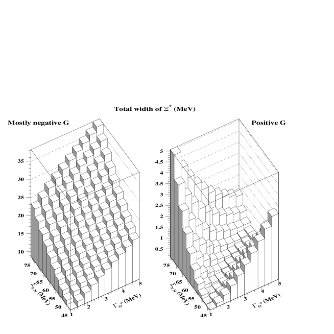
Figure 15: The total width of $\Xi_{\overline{10}}$ as a function of $\Gamma_{\Theta^{+}}$ and $\Sigma_{\pi\,N}$ in the presence of the mixing with the 27-plet. The two plots correspond to the positive and mostly negative $G_{\overline{10}}$ solutions.

In what follows, we repeat the analysis of the antidecuplet decays including the 27-plet contribution. We start with the total width of $\Xi_{\overline{10}}$. Figure 15 presents $\Gamma_{\Xi_{\overline{10}}}$ as a function of $\Gamma_{\Theta^{+}}$ and $\Sigma_{\pi\,N}$ for the two possible solutions for $G_{\overline{10}}$. In agreement with the analysis of 27plet , the mixing with the 27-plet is rather important for the decays of the $\Xi_{\overline{10}}$.

Note that the positive $G_{\overline{10}}$ solution at large $\Gamma_{\Theta^{+}}$ and $\Sigma_{\pi\,N}$ results in the values of $\Gamma_{\Xi_{\overline{10}}}$ which are higher than the present upper limit on the total width of $\Xi_{\overline{10}}$. However, until the existence of $\Xi_{\overline{10}}$ and its properties receive firmer experimental support BABAR ; NA49:critique , one should not make any quantitative statements about which values $\Gamma_{\Theta^{+}}$, $\Sigma_{\pi\,N}$, $\theta_{2}$ and $\theta_{3}$ are appropriate for the sufficiently narrow $\Gamma_{\Xi_{\overline{10}}}$.

B.3 Decays of $N_{\overline{10}}$

We found that the mixing with the 27-plet insignificantly lowers the total width of $N_{\overline{10}}$ and, hence, Fig. 3 changes only little when the 27-plet admixture is included. The change is small because, in general, $\Gamma_{N_{\overline{10}}}$ receives a dominant contribution from $\Gamma_{N_{\overline{10}}\to\Delta\,\pi}$, which is insensitive to the 27-plet contribution, see Eqs. 24.

Figures 16, 17 and 18 present the $\Gamma_{N_{\overline{10}}\to N\,\pi}$, $\Gamma_{N_{\overline{10}}\to N\,\eta}$ and $\Gamma_{N_{\overline{10}}\to\Lambda\,K}$ partial decay widths in the presence of the mixing with the 27-plet as functions of the $\theta_{2}$ and $\theta_{3}$ mixing angles at $\Gamma_{\Theta^{+}}=1$ and 5 MeV and at $\Sigma_{\pi\,N}=45$ and 75 MeV. In each plot, the four upper panels correspond to the positive $G_{\overline{10}}$ solution; the four lower panels correspond to the mostly negative $G_{\overline{10}}$ solution. Note that the $\Gamma_{N_{\overline{10}}\to\Delta\,\pi}$ is presented in Fig. 5.

An examination of Figs. 16, 17 and 18 shows that the difference between the predicted partial widths using the two solutions for $G_{\overline{10}}$ is dramatic: The use of the mostly negative $G_{\overline{10}}$ instead of the positive $G_{\overline{10}}$ increases $\Gamma_{N_{\overline{10}}\to N\,\pi}$ and reduces $\Gamma_{N_{\overline{10}}\to N\,\eta}$ and $\Gamma_{N_{\overline{10}}\to\Lambda\,K}$. However, we shall still be able to find regions of the $\theta_{2}$ and $\theta_{3}$ mixing angles where $\Gamma_{N_{\overline{10}}\to N\,\eta}>\Gamma_{N_{\overline{10}}\to N\,\pi}$.

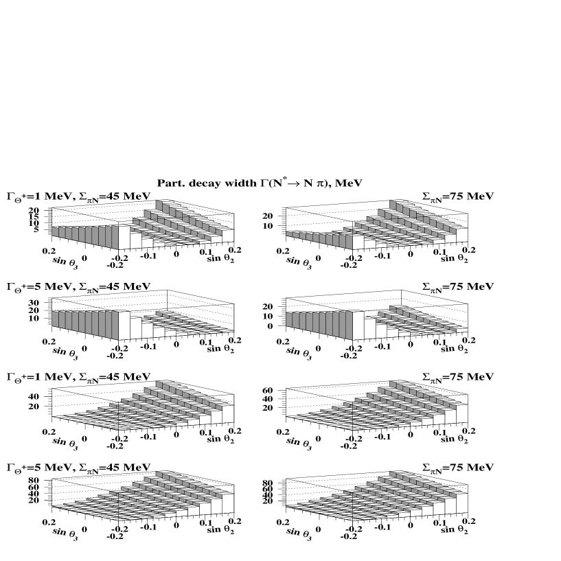
Figure 16: $\Gamma_{N_{\overline{10}}\to N\,\pi}$ as a function of $\theta_{2}$ and $\theta_{3}$ in the presence of the mixing with the 27-plet. The four upper panels correspond to the positive $G_{\overline{10}}$ solution; the four lower panels correspond to the mostly negative $G_{\overline{10}}$ solution.

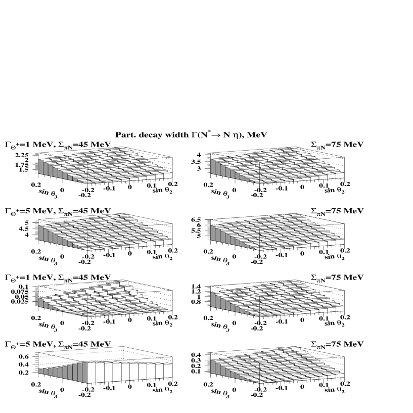
Figure 17: $\Gamma_{N_{\overline{10}}\to N\,\eta}$ as a function of $\theta_{2}$ and $\theta_{3}$ in the presence of the mixing with the 27-plet. The four upper panels correspond to the positive $G_{\overline{10}}$ solution; the four lower panels correspond to the mostly negative $G_{\overline{10}}$ solution.

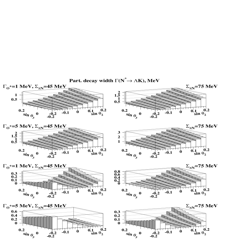
Figure 18: $\Gamma_{N_{\overline{10}}\to\Lambda\,K}$ as a function of $\theta_{2}$ and $\theta_{3}$ in the presence of the mixing with the 27-plet. The four upper panels correspond to the positive $G_{\overline{10}}$ solution; the four lower panels correspond to the mostly negative $G_{\overline{10}}$ solution.

We are interested in the values of the $\theta_{2,3}$ mixing angles which correspond to $\Gamma_{N_{\overline{10}}\to N\,\pi}\leq 1$ MeV. Figure 19 presents the allowed regions of $\sin\theta_{2,3}$ in the presence of the $\Gamma_{N_{\overline{10}}\to N\,\pi}\leq 1$ MeV condition. At given $\sin\theta_{2}$, the two solid curves present the maximal and minimal values of $\sin\theta_{3}$. The four upper panels correspond to the positive $G_{\overline{10}}$ solution; the four lower panels correspond to the mostly negative $G_{\overline{10}}$ solution.

Figure 19: The regions of the $\theta_{2}$ and $\theta_{2}$ mixing angles allowed by the $\Gamma_{N_{\overline{10}}\to N\,\pi}\leq 1$ MeV condition in the presence of the mixing with the 27-plet. The four upper panels correspond to the positive $G_{\overline{10}}$ solution; the four lower panels correspond to the mostly negative $G_{\overline{10}}$ solution.

Figures 20, 21, 22 and 23 present the $\Gamma_{N_{\overline{10}}\to N\,\pi}$, $\Gamma_{N_{\overline{10}}\to N\,\eta}$, $\Gamma_{N_{\overline{10}}\to\Lambda\,K}$ and $\Gamma_{N_{\overline{10}}\to\Delta\,\pi}$ partial decay widths in the region of $\theta_{2}$ and $\theta_{3}$ where $\Gamma_{N_{\overline{10}}\to N\,\pi}\leq 1$ MeV.

For the positive $G_{\overline{10}}$ solution, the 27-plet contribution lowers $\Gamma_{N_{\overline{10}}\to N\,\pi}$. As a result, the kinematic region where $\Gamma_{N_{\overline{10}}\to N\,\pi}\leq 1$ MeV (four upper panels in Fig. 20) is somewhat wider than in Fig. 7. In addition, the region is shifted towards positive $\sin\theta_{2}$. As to the mostly negative $G_{\overline{10}}$ solution, the 27-plet contribution increases $\Gamma_{N_{\overline{10}}\to N\,\pi}$ and, thus, makes the region $\Gamma_{N_{\overline{10}}\to N\,\pi}\leq 1$ rather narrow. The allowed region corresponds to large and negative $\sin\theta_{2}$, see four lower panels in Fig. 20.

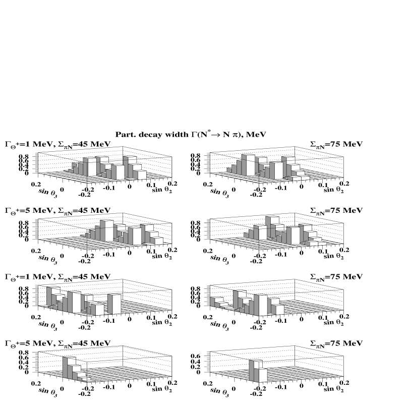
Figure 20: $\Gamma_{N_{\overline{10}}\to N\,\pi}$ as a function of $\theta_{2}$ and $\theta_{3}$ in the presence of the mixing with the 27-plet. The decay width is shown only where $\Gamma_{N_{\overline{10}}\to N\,\pi}\leq 1$ MeV. The four upper panels correspond to the positive $G_{\overline{10}}$ solution; the four lower panels correspond to the mostly negative $G_{\overline{10}}$ solution.

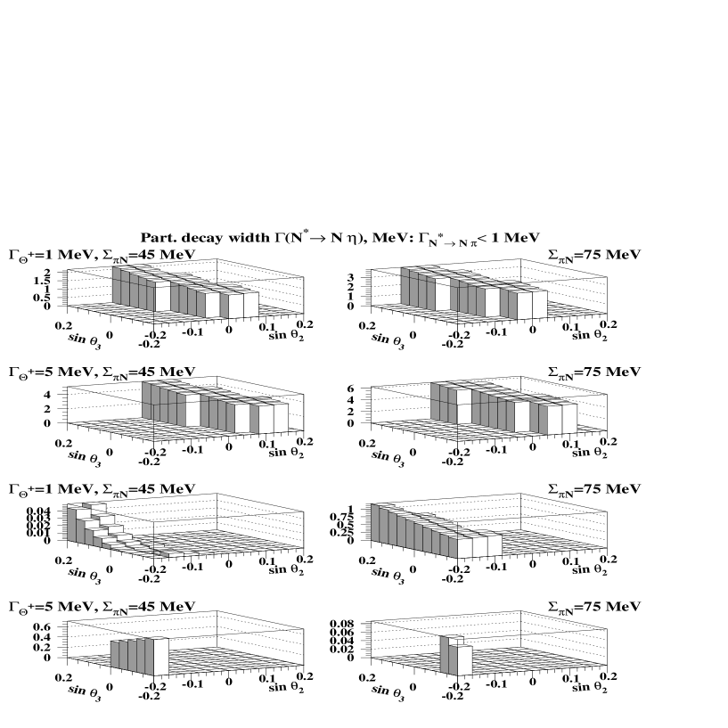
Figure 21: $\Gamma_{N_{\overline{10}}\to N\,\eta}$ as a function of $\theta_{2}$ and $\theta_{3}$ in the presence of the mixing with the 27-plet. The decay width is shown only where $\Gamma_{N_{\overline{10}}\to N\,\pi}\leq 1$ MeV. The four upper panels correspond to the positive $G_{\overline{10}}$ solution; the four lower panels correspond to the mostly negative $G_{\overline{10}}$ solution.

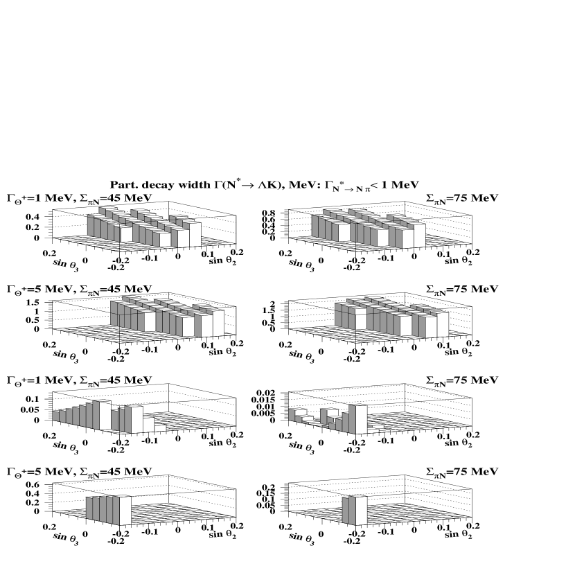
Figure 22: $\Gamma_{N_{\overline{10}}\to\Lambda\,K}$ as a function of $\theta_{2}$ and $\theta_{3}$ in the presence of the mixing with the 27-plet. The decay width is shown only where $\Gamma_{N_{\overline{10}}\to N\,\pi}\leq 1$ MeV. The four upper panels correspond to the positive $G_{\overline{10}}$ solution; the four lower panels correspond to the mostly negative $G_{\overline{10}}$ solution.

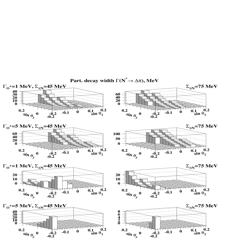
Figure 23: $\Gamma_{N_{\overline{10}}\to\Delta\,\pi}$ as a function of $\theta_{2}$ and $\theta_{3}$ in the presence of the mixing with the 27-plet. The decay width is shown only where $\Gamma_{N_{\overline{10}}\to N\,\pi}\leq 1$ MeV. The four upper panels correspond to the positive $G_{\overline{10}}$ solution; the four lower panels correspond to the mostly negative $G_{\overline{10}}$ solution.

Turning to the $\Gamma_{N_{\overline{10}}\to N\,\eta}$ partial decay width (Fig. 21), we notice that the positive $G_{\overline{10}}$ solution corresponds to the $\Gamma_{N_{\overline{10}}\to N\,\eta}$, which is of the order of several MeV. On the other hand, among the cases corresponding to the mostly negative $G_{\overline{10}}$ solution (four lower panels of Fig. 21), only the $\Gamma_{\Theta^{+}}=1$ MeV and $\Sigma_{\pi\,N}=75$ MeV case fits our qualitative picture of the $N_{\overline{10}}$ decays, which assumes that while the $\Gamma_{N_{\overline{10}}\to N\,\pi}$ is suppressed and $\Gamma_{N_{\overline{10}}\to\Lambda\,K}$ is possibly suppressed, $\Gamma_{N_{\overline{10}}\to N\,\eta}$ is sizable.

We explained in Sect. III that the STAR result on the $\Lambda\,K_{S}$ invariant mass spectrum STAR can be interpreted as an indication that $\Gamma_{N_{\overline{10}}\to\Lambda\,K}$ is possibly suppressed. Therefore, all cases considered in Fig. 22 (except maybe for the $\Gamma_{\Theta^{+}}=5$ MeV and positive $G_{\overline{10}}$ case) fit well the hypothesis of the suppressed $\Gamma_{N_{\overline{10}}\to\Lambda\,K}$.

The $\Gamma_{N_{\overline{10}}\to\Delta\,\pi}$ is a steeply rising function of $\theta_{2}$. For the positive $G_{\overline{10}}$ solution, the 27-plet admixture shifts the range of $\sin\theta_{2,3}$ allowed by the $\Gamma_{N_{\overline{10}}\to N\,\pi}\leq 1$ MeV condition towards positive $\sin\theta_{2}$. As a results, the values of $\Gamma_{N_{\overline{10}}\to\Delta\,\pi}$ in four upper panels of Fig. 23 are significantly higher than in Fig. 8. This should be contrasted with the predicted much lower $\Gamma_{N_{\overline{10}}\to\Delta\,\pi}$, which corresponds to the mostly negative $G_{\overline{10}}$ solution, see the lower four panels of Fig. 23.

The sum of the considered two-hadron partial decays widths of $N_{\overline{10}}$, in the presence of the $\Gamma_{N_{\overline{10}}\to N\,\pi}\leq 1$ MeV condition and the mixing with the 27-plet, varies in the interval summarized in Table 3. The first value corresponds to the positive $G_{\overline{10}}$ solution; the value in the parenthesis corresponds to the mostly negative $G_{\overline{10}}$ solution.

$\Gamma_{\Theta^{+}}$ (MeV)	$\Sigma_{\pi\,N}$ (MeV)	$\Gamma_{N_{\overline{10}}}^{{\rm 2-body,min}}$ (MeV)	$\Gamma_{N_{\overline{10}}}^{{\rm 2-body,max}}$ (MeV)
1	45	1.9 (0.1)	52 (37)
1	75	4.3 (0.8)	103 (38)
5	45	5.7 (3.4)	97 (55)
5	75	17 (1.3)	157 (14)

Table 3: The range of change of $\Gamma_{N_{\overline{10}}}^{{\rm 2-body}}$. The first value corresponds to the positive $G_{\overline{10}}$ solution; the value in the parenthesis corresponds to the mostly negative $G_{\overline{10}}$ solution.

In summary, the additional mixing with the 27-plet does not change our qualitative picture of the $N_{\overline{10}}$ decays when we use the positive solution for the $G_{\overline{10}}$ coupling constant. The picture consists in the following observations: $\Gamma_{N_{\overline{10}}\to N\,\pi}$ is suppressed; $\Gamma_{N_{\overline{10}}\to\Lambda\,K}$ is possibly suppressed; $\Gamma_{N_{\overline{10}}\to N\,\eta}$ is sizable; $\Gamma_{N_{\overline{10}}\to\Delta\,\pi}$ is not too large such that $\Gamma_{N_{\overline{10}}}$ is of the order of 10-20 MeV.

Using the mostly negative solution for the $G_{\overline{10}}$ coupling constant, the above mentioned picture emerges only at $\Gamma_{\Theta^{+}}=1$ MeV and $\Sigma_{\pi\,N}=75$ MeV. A particular feature of this scenario is a possibly very narrow $N_{\overline{10}}$ with a vanishingly small $\Gamma_{N_{\overline{10}}\to\Lambda\,K}$.

B.4 Decays of $\Sigma_{\overline{10}}$

The total width of $\Sigma_{\overline{10}}$ is presented in Fig. 24. A comparison with Fig. 9 reveals that using the positive $G_{\overline{10}}$ solution, the 27-plet makes an insignificant contribution at small values of $\Gamma_{\Theta^{+}}$. On the other hand, at $\Sigma_{\pi\,N}=75$ MeV, the 27-plet contribution alters the pattern of the $\theta_{2}$ and $\theta_{3}$ dependence and noticeably changes the size of $\Gamma_{\Sigma_{\overline{10}}}$. In addition, our predictions for $\Gamma_{\Sigma_{\overline{10}}}$ are very different when we use the positive and mostly native solutions for $G_{\overline{10}}$.

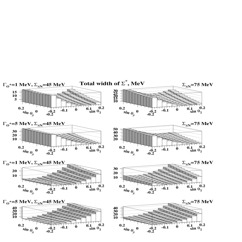
Figure 24: The total width of $\Sigma_{\overline{10}}$ as a function of $\theta_{2}$ and $\theta_{3}$ in the presence of the mixing with the 27-plet. The four upper panels correspond to the positive $G_{\overline{10}}$ solution; the four lower panels correspond to the mostly negative $G_{\overline{10}}$ solution.

The $\Gamma_{\Sigma_{\overline{10}}\to\Lambda\,\pi}$, $\Gamma_{\Sigma_{\overline{10}}\to\Sigma\,\pi}$ and $\Gamma_{\Sigma_{\overline{10}}\to N\,K}$ partial decay widths in the presence of the mixing with the 27-plet are presented in Figs. 25, 26 and 27. As can be readily seen from a comparison with Figs. 10 and 11, the influence of the 27-plet is dramatic: Both the patterns and the absolute values of the predicted partial decay widths are different.

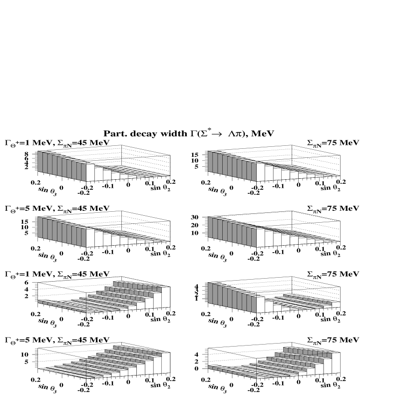
Figure 25: $\Gamma_{\Sigma_{\overline{10}}\to\Lambda\,\pi}$ as a function of $\theta_{2}$ and $\theta_{3}$ in the presence of the mixing with the 27-plet. The four upper panels correspond to the positive $G_{\overline{10}}$ solution; the four lower panels correspond to the mostly negative $G_{\overline{10}}$ solution.

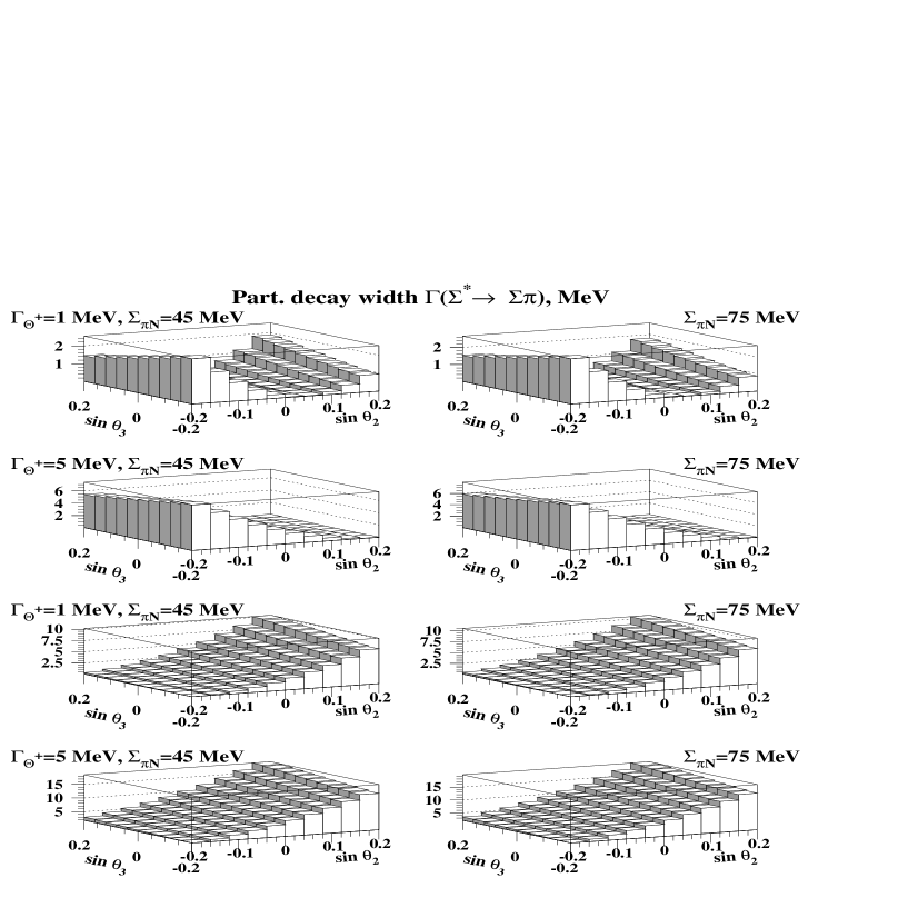
Figure 26: $\Gamma_{\Sigma_{\overline{10}}\to\Sigma\,\pi}$ as a function of $\theta_{2}$ and $\theta_{3}$ in the presence of the mixing with the 27-plet. The four upper panels correspond to the positive $G_{\overline{10}}$ solution; the four lower panels correspond to the mostly negative $G_{\overline{10}}$ solution.

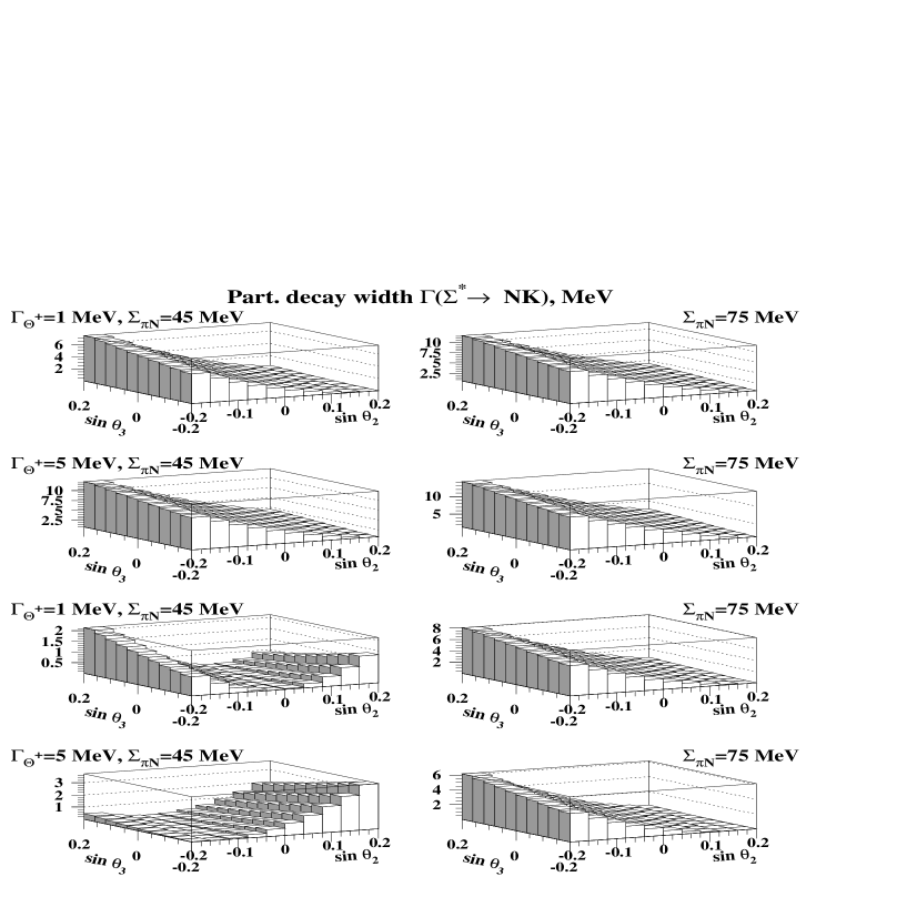
Figure 27: $\Gamma_{\Sigma_{\overline{10}}\to N\,K}$ as a function of $\theta_{2}$ and $\theta_{3}$ in the presence of the mixing with the 27-plet. The four upper panels correspond to the positive $G_{\overline{10}}$ solution; the four lower panels correspond to the mostly negative $G_{\overline{10}}$ solution.

Next we examine the considered partial decay widths of $\Sigma_{\overline{10}}$ in the domain of the $\theta_{2}$ and $\theta_{3}$ mixing angles where $\Gamma_{N_{\overline{10}}\to N\,\pi}\leq 1$ MeV. The results are presented in Figs. 28, 29, 30 and 31.

First we consider the case of the positive $G_{\overline{10}}$ coupling constant. As seen from a comparison of Figs. 28 and 30, $\Gamma_{\Sigma_{\overline{10}}\to\Lambda\,\pi}>\Gamma_{\Sigma_{\overline{10}}\to N\,K}$, which makes it difficult or even impossible to identify $\Sigma_{\overline{10}}$ with $\Sigma(1770)$ because the data suggests that $Br(\Sigma(1770)\to N\,\overline{K})$ is several times larger than $Br(\Sigma(1770)\to\Lambda\,\pi)$.

Turning to the mostly negative $G_{\overline{10}}$ solution, we see that the emerging pattern of the $\Sigma_{\overline{10}}$ decays reminds that of $\Sigma(1770)$: The $\Gamma_{\Sigma_{\overline{10}}\to N\,K}$ partial decay widths is several times larger than $\Gamma_{\Sigma_{\overline{10}}\to\Lambda\,\pi}$ and $\Gamma_{\Sigma_{\overline{10}}\to\Sigma\,\pi}$.

Taking the sum of the considered two-hadron partial decay widths of $\Sigma_{\overline{10}}$, we find that in presence of the $\Gamma_{N_{\overline{10}}\to N\,\pi}\leq 1$ MeV constraint and mixing with the 27-plet, $\Gamma_{\Sigma_{\overline{10}}}^{{\rm 2-body}}$ varies in the interval summarized in Table 4.

$\Gamma_{\Theta^{+}}$ (MeV)	$\Sigma_{\pi\,N}$ (MeV)	$\Gamma_{\Sigma_{\overline{10}}}^{{\rm 2-body,min}}$ (MeV)	$\Gamma_{\Sigma_{\overline{10}}}^{{\rm 2-body,max}}$ (MeV)
1	45	1.2 (1.5)	13 (4.2)
1	75	7.8 (5.3)	30 (17)
5	45	3.8 (3.1)	21 (6.8)
5	75	13 (6.9)	40 (8.2)

Table 4: The range of change of $\Gamma_{\Sigma_{\overline{10}}}^{{\rm 2-body}}$. The first value corresponds to the positive $G_{\overline{10}}$ solution; the value in the parenthesis corresponds to the mostly negative $G_{\overline{10}}$ solution.

In summary, the antidecuplet mixing with a 27-plet significantly affects the $\Sigma_{\overline{10}}$ decays. Using the positive $G_{\overline{10}}$ solution, we predict that $\Gamma_{\Sigma_{\overline{10}}\to\Lambda\,\pi}>\Gamma_{\Sigma_{\overline{10}}\to N\,K}$ and that the both partial widths of the order of 5-15 MeV. With the mostly negative $G_{\overline{10}}$ solution, we obtain a rather narrow $\Sigma_{\overline{10}}$ with decays properties qualitatively reminding those of $\Sigma(1770)$. Of course, our $\Sigma_{\overline{10}}$ is much narrower than $\Sigma(1770)$.

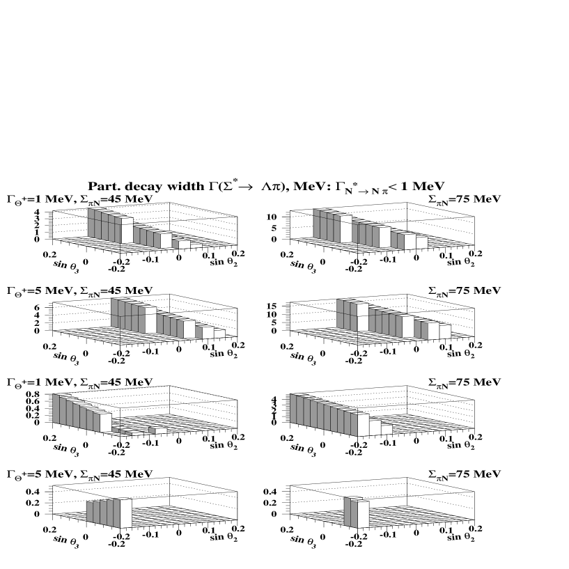
Figure 28: $\Gamma_{\Sigma_{\overline{10}}\to\Lambda\,\pi}$ as a function of $\theta_{2}$ and $\theta_{3}$ in the presence of the mixing with the 27-plet. The decay width is shown only where $\Gamma_{N_{\overline{10}}\to N\,\pi}\leq 1$ MeV. The four upper panels correspond to the positive $G_{\overline{10}}$ solution; the four lower panels correspond to the mostly negative $G_{\overline{10}}$ solution.

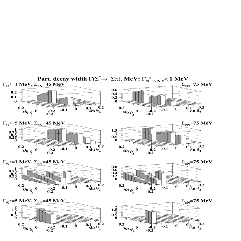
Figure 29: $\Gamma_{\Sigma_{\overline{10}}\to\Sigma\,\pi}$ as a function of $\theta_{2}$ and $\theta_{3}$ in the presence of the mixing with the 27-plet. The decay width is shown only where $\Gamma_{N_{\overline{10}}\to N\,\pi}\leq 1$ MeV. The four upper panels correspond to the positive $G_{\overline{10}}$ solution; the four lower panels correspond to the mostly negative $G_{\overline{10}}$ solution.

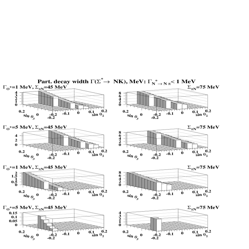
Figure 30: $\Gamma_{\Sigma_{\overline{10}}\to N\,\overline{K}}$ as a function of $\theta_{2}$ and $\theta_{3}$ in the presence of the mixing with the 27-plet. The decay width is shown only where $\Gamma_{N_{\overline{10}}\to N\,\pi}\leq 1$ MeV. The four upper panels correspond to the positive $G_{\overline{10}}$ solution; the four lower panels correspond to the mostly negative $G_{\overline{10}}$ solution.

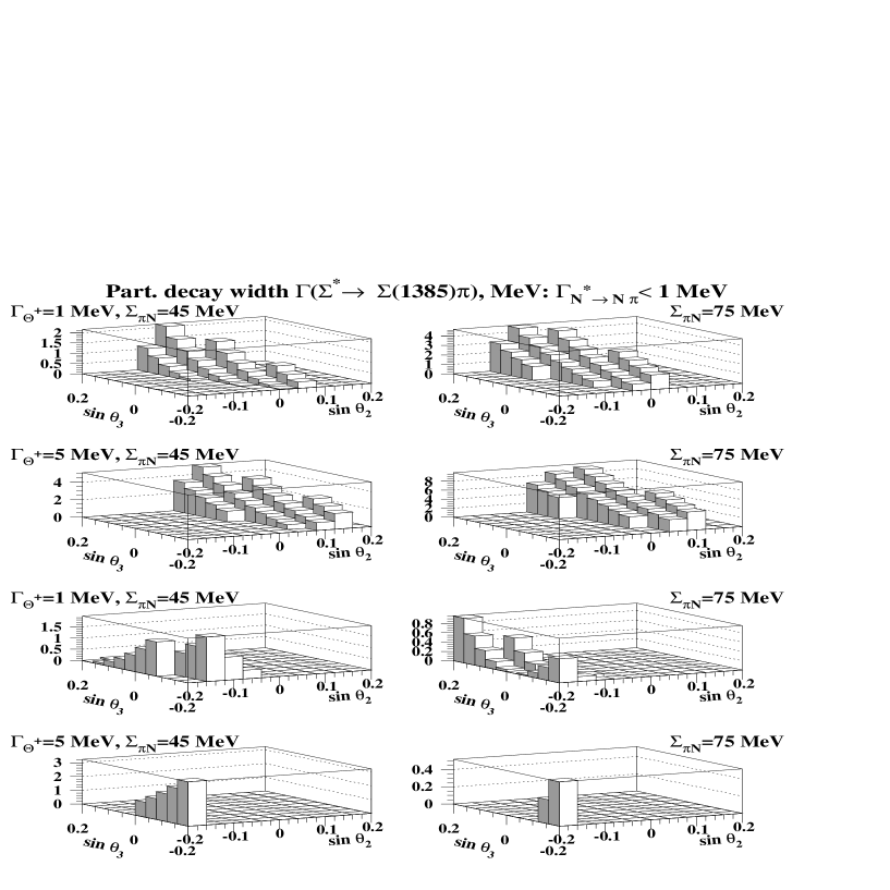
Figure 31: $\Gamma_{\Sigma_{\overline{10}}\to\Sigma(1385)\,\pi}$ as a function of $\theta_{2}$ and $\theta_{3}$ in the presence of the mixing with the 27-plet. The decay width is shown only where $\Gamma_{N_{\overline{10}}\to N\,\pi}\leq 1$ MeV. The four upper panels correspond to the positive $G_{\overline{10}}$ solution; the four lower panels correspond to the mostly negative $G_{\overline{10}}$ solution.

References

- (1) M. Gell-Mann and Y. Ne’eman, The Eightfold Way, W.A. Benjamin, Inc., Amsterdam and New York, 1964.
- (2) J.J.J. Kokkedee, The quark model, W.A. Benjamin, Inc., Amsterdam and New York, 1969.
- (3) F.E. Close, An introduction to quarks and partons, Academic Press, London, 1979.
- (4) N.P. Samios, M. Goldberg, and B.T. Meadows, Rev. Mod. Phys. 46, 49 (1974).
- (5) Spring-8 Collab., T. Nakano et al., Phys. Rev. Lett. 91, 012002 (2003).
- (6) DIANA Collab., V.V. Barmin et al., Yad. Fiz. 66, 1763 (2003) [Phys. Atom. Nucl. 66, 1715 (2003)] [hep-ex/0304040].
- (7) CLAS Collab., S. Stepanyan et al., Phys. Rev. Lett. 91, 252001 (2003) [hep-ex/0307018].
- (8) SAPHIR Collab., J. Barth et al., Phys. Lett. B 572, 127 (2003) [hep-ex/0307083].
- (9) A.E. Asratyan, A.G. Dolgolenko and M.A. Kubantsev, Yad. Fiz. 67, 704 (2004) [Phys. At. Nucl. 67, 682 (2004)] [hep-ex/0309042].
- (10) CLAS Collab. V. Kubarovsky et al., Phys. Rev. Lett. 92, 032001 (2004); Erratum-ibid. 92, 049902 (2004) [hep-ex/0311046].
- (11) HERMES Collab., A. Airapetian et al., Phys. Lett. B 585, 213 (2004) [hep-ex/0312044].
- (12) SVD Collab., A. Aleev et al., hep-ex/0401024, submitted to Yad. Fiz.
- (13) COSY-TOF Collab., M. Abdel-Bary et al., Phys. Lett. B 595, 127 (2004) [hep-ex/0403011].
- (14) ZEUS Collab., S. Chekanov et al., Phys. Lett. B 591, 7 (2004) [hep-ex/0403051].
- (15) GRAAL Collab., C. Schaerf, talk at the Pentaquark 2003 workshop, Jefferson Lab, Newport News, Virginia, November 2003.
- (16) R. Togoo et al., Proc. Mongolian Acad. Sci., 4, 2 (2003).
- (17) Yu.A. Troyan, et al., hep-ex/0404003.
- (18) NA49 Collab., C. Alt et al., Phys. Rev. Lett. 92, 042003 (2004) [hep-ex/0310014].
- (19) BES Collab., J.Z. Bai et al., Phys. Rev. D 70, 012004 (2004) [hep-ex/0402012].
- (20) ALEPH Collab., S. Schael et al., Phys. Lett. B 599, 1 (2004).
- (21) BABAR Collab., B. Aubert et al., hep-ex/0408064 and hep-ex/0408037.
- (22) HERA-B Collab., I. Abt et al., Phys. Rev. Lett. 93, 212003 (2004) [hep-ex/0408048].
- (23) D. Litvintsev for the CDF Collab., hep-ex/0410024.
- (24) K. Stenson, for FOCUS Collab., hep-ex/0412021.
- (25) Belle Collab., K. Abe et al., hep-ex/0409010.
- (26) C. Pinkenburg for the PHENIX Collab., J. Phys. G 30, S1201 (2004) [nucl-ex/0404001].
- (27) D. Diakonov, V. Petrov and M. Polyakov, Z. Phys. A 359, 305 (1997).
-
(28)
J. Ellis, M. Karliner, M. Praszalowicz, JHEP 0405 (2004) 002
[hep-ph/0401127];
M. Praszalowicz, Acta Phys. Polon. B 35 (2004) 1625 [hep-ph/0402038]. - (29) R.A. Arndt, I.I. Strakovsky and R.L. Workman, Phys. Rev. C 68, 042201(R) (2003) [nucl-th/0308012]; Erratum-ibid. C 69, 019901 (2004).
- (30) A. Casher and S. Nussinov. Phys. Lett. B 578, 124 (2004) [hep-ph/0309208].
- (31) J. Haidenbauer and G. Krein, Phys. Rev. C 68, 052201 (2003) [hep-ph/0309243].
- (32) R.N. Cahn and G.H. Trilling, Phys. Rev. D 69, 011501(R) (2004) [hep-ph/031124].
- (33) W.R. Gibbs, Phys. Rev. C 70, 045208 (2004) [nucl-th/0405024].
- (34) A. Sibirtsev, J. Haidenbauer, S. Krewald, and Ulf-G. Meissner, Phys. Lett. B 599, 230 (2004) [hep-ph/0405099].
- (35) A. Sibirtsev, J. Haidenbauer, S. Krewald, and Ulf-G. Meissner, nucl-th/0407011.
- (36) R.L. Jaffe and F. Wilczek, Phys. Rev. Lett. 91, 232003 (2003) [hep-ph/0307341].
- (37) Fl. Stanchu, hep-ph/0410033.
- (38) D. Faiman, Phys. Rev. D 15, 854 (1977).
- (39) T. Cohen, Phys. Rev. D 70, 074023 (2004) [hep-ph/0402056].
- (40) The Review of Particle Physics 2004, Particle Data Group, S. Eidelman et al. Phys. Lett. B. 592 (2004) 1.
- (41) D. Diakonov and V. Petrov, Phys. Rev. D 69, 094011 (2004) [hep-ph/310212].
- (42) V. Guzey and M. Polyakov, in preparation.
- (43) P.N. Dobson, Jr., S. Pakvasa, and S.F. Tuan, Hadronic J. 1, 476 (1978).
- (44) J.J. de Swart, Rev. Mod. Phys. 35, 916 (1963).
- (45) R.A. Arndt, Ya.I. Azimov, M.V. Polyakov, I.I. Strakovsky, and R.L. Workman, Phys. Rev. C 69, 035208 (2004) [nucl-th/0312126].
-
(46)
The discussion of the phase space factor of the
ground-state decuplet is recommended to be read in
the presented order:
R.L. Jaffe, Eur. Phys. J. C 35, 221 (2004);
D. Diakonov, V. Petrov and M. Polyakov, hep-ph/0404212;
R.L. Jaffe, hep-ph/0405268. - (47) G. Höhler, Pion–Nucleon Scattering, Landoldt–Börnstein Vol. I/9b2, edited by H. Schopper (Springer Verlag, 1983).
- (48) J. Gasser, H. Leutwyler and M.E. Sainio, Phys. Lett. B 253, 252 (1991).
- (49) M.M. Pavan, I.I. Strakovsky, R.L. Workman, and R.A. Arndt, PiN Newslett. 16, 110 (2002) [hep-ph/0111066].
- (50) V. Kuznetsov for the GRAAL Collab., hep-ex/0409032.
- (51) S. Kabana for the STAR Collab., hep-ex/0406032.
- (52) W. Lorenzon for the HERMES Collab., hep-ex/0411027.
- (53) G.P. Gopal et al., Nucl. Phys. B 199, 362 (1977).
- (54) A. Hosaka et al., hep-ph/0411311.
- (55) H.G. Fischer and S. Wenig, Eur. Phys. J. C 37, 133 (2004) [hep-ex/0401014].