The MSW effect and Matter Effects in Neutrino Oscillations

A. Yu. Smirnov^2,3

(2) The Abdus Salam International Centre for Theoretical Physics, I-34100 Trieste, Italy
(3) Institute for Nuclear Research of Russian Academy of Sciences, Moscow 117312, Russia

The MSW (Mikheyev-Smirnov-Wolfenstein) effect is the adiabatic or partially adiabatic neutrino flavor conversion in medium with varying density. The main notions related to the effect, its dynamics and physical picture are reviewed. The large mixing MSW effect is realized inside the Sun providing the solution of the solar neutrino problem. The small mixing MSW effect driven by the 1-3 mixing can be realized for the supernova (SN) neutrinos. Inside the collapsing stars new elements of the MSW dynamics may show up: the non-oscillatory transition, non-adiabatic conversion, time dependent adiabaticity violation induced by shock waves. Effects of the resonance enhancement and the parametric enhancement of oscillations can be realized for the atmospheric and accelerator neutrinos in the Earth. Precise results for neutrino oscillations in the low density medium with arbitrary density profile are presented and the attenuation effect is described. The area of applications is the solar and SN neutrinos inside the Earth, and the results are crucial for the neutrino oscillation tomography.

1 Introduction

Variety of matter effects [1] on propagation of mixed neutrinos [2, 3] depends on (i) channel of mixing - the type of neutrino states involved: active, sterile, mass eigenstates, etc.; (ii) density profile: constant, monotonous, periodic, fluctuating; (iii) properties of medium: polarization, motion, chemical composition (thermal bath and neutrino gases are special cases); (iv) presence of new non-standard neutrino interactions.

Dynamics of the matter effects can be classified by degrees of freedom involved. In the $2\nu$ case, an arbitrary neutrino state can be expressed in terms of the eigenstates of the instantaneous Hamiltonian, $\nu_{1m}$ and $\nu_{2m}$, as

$$\nu(x)=\cos\theta_{a}\nu_{1m}+\sin\theta_{a}\nu_{2m}e^{i\Phi_{m}}~{},$$ (1)

where

• $\theta_{a}=\theta_{a}(x)$ determines the admixtures of eigenstates in $\nu(x)$;

• $\Phi_{m}(x)$ is the phase difference between the two eigenstates (phase of oscillations):

  $$\Phi_{m}(x)=\int_{x_{0}}^{x}\Delta Hdt^{\prime},$$ (2)

  here $\Delta H\equiv H_{2m}-H_{1m}$ is the difference of eigenvalues. Eq. (2) gives the adiabatic phase, an additional contributions can be related to non-adiabaticity and topology.

• The mixing angle in matter, $\theta_{m}$, defined as $\langle\nu_{e}|\nu_{1m}\rangle\equiv\cos\theta_{m}$, $\langle\nu_{e}|\nu_{2m}\rangle\equiv\sin\theta_{m}$, etc., determines the flavor contents (or flavors) of the eigenstates. The angle is the function of matter density $n_{e}(x)$: $\theta_{m}=\theta_{m}(n_{e}(x))$.

Besides these, the effects of absorption and loss of the coherence can change the normalization of the eigenstates or suppress interference.

Different processes are associated with these degrees of freedom. In particular, in pure form the oscillations [2, 3, 4, 1, 5] are the effect of the monotonous phase difference increase $\Phi_{m}$, which occurs in the uniform medium. In contrast, the MSW effect [1, 6] is associated to the change of flavors of the eigenstates (change of $\theta_{m}(x)$) in the nonuniform medium. In general, an interplay of different effects occurs which is induced by simultaneous operation of several degrees of freedom.

In this paper I will discuss only few effects selected on the following ground: usual massive neutrinos with the flavor mixing and standard weak interactions; the effects in the Sun, collapsing stars and the Earth; the effects which are realized in Nature or have a good chance to be realized and established in our future studies.

2 The MSW effect.

The MSW effect [1, 6] is the adiabatic or partially adiabatic neutrino flavor conversion in medium with varying density. The flavor of neutrino state follows the density change. Here I review the main notions related to the effect and describe its dynamics.

2.1 Main notions

1. Refraction.   At low energies the elastic forward scattering only is relevant in most of applications  [1, 7]. It can be described by the potential, $V$, or equivalently, the refraction index: $n_{ref}-1={V}/{p}$.

The difference of potentials (for a single neutrino) in different spatial points $V=V(x)$ leads to the “neutrino optics” phenomena such as reflection, complete internal reflection, banding of neutrino trajectories, focusing by the stars, etc.. The values of refraction index are very close to unit, e.g.,: $n_{ref}-1=10^{-20}$ inside the Earth, $10^{-18}$ inside the Sun, $10^{-6}$ in the neutron stars. So, the “neutrino lenses” should be of the astrophysical size.

The difference of potentials for different neutrinos, $\nu_{e}$ and $\nu_{a}$: $V\equiv V_{e}-V_{a}$ influences evolution of mixed neutrinos (even for constant potentials). In usual matter the difference is due to the charged current scattering of $\nu_{e}$ on electrons ($\nu_{e}e\rightarrow\nu_{e}e$) [1]:

$$V\equiv V_{e}-V_{a}=\sqrt{2}G_{F}n_{e}~{},$$ (3)

where $G_{F}$ is the Fermi coupling constant and $n_{e}$ is the number density of electrons. It leads to appearance of additional phase in the neutrino system: $\Delta\phi_{matter}\equiv(V_{e}-V_{a})t$. The distance over which this “matter” phase equals $2\pi$ determines the refraction length:

$$l_{0}\equiv\frac{2\pi}{V_{e}-V_{a}}=\frac{\sqrt{2}\pi}{G_{F}n_{e}}.$$ (4)

2. Eigenstates and mixing in matter.  In the presence of matter the Hamiltonian of system changes: $H_{0}\rightarrow H=H_{0}+V,$ where $H_{0}$ is the Hamiltonian in vacuum. Correspondingly, the eigenstates and the eigenvalues of $H$ change: $\nu_{1},\nu_{2}\rightarrow\nu_{1m},\nu_{2m}$, $m_{1}^{2}/2E,m_{2}^{2}/2E\rightarrow H_{1m},H_{2m}$. Here $\nu_{1}$ and $\nu_{2}$ are the mass eigenstates with masses $m_{1}$ and $m_{2}$.

The mixing in matter is defined with respect to the eigenstates $\nu_{1m}$ and $\nu_{2m}$. Similarly to the vacuum case, the mixing angle in matter, $\theta_{m}$, determines relations between the eigenstates in matter and the flavor states: $\nu_{e}\equiv\cos\theta_{m}\nu_{1m}+\sin\theta_{m}\nu_{2m}$, etc.. In matter, both the eigenstates and eigenvalues, and consequently, the mixing angle depend on matter density and neutrino energy.

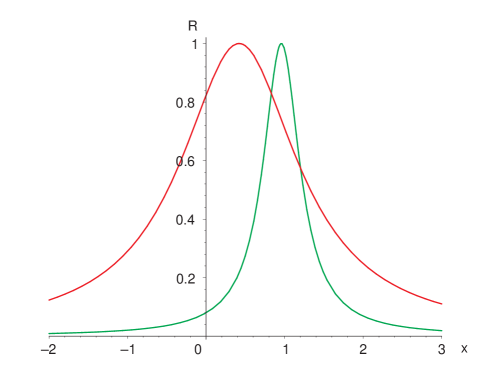
Figure 1: The dependence of the effective mixing parameter $R\equiv\sin^{2}2\theta_{m}$ on $x\equiv l_{\nu}/l_{0}\propto En_{e}$ for two different values of the vacuum mixing: $\sin^{2}2\theta=0.825$ (black, red) which is the LMA mixing and $\tan^{2}\theta=0.08$ (grey, green). The semi-plane $x<0$ corresponds to the antineutrino channel.

3. Resonance.  Dependence of the effective mixing parameter in matter, $R\equiv\sin^{2}2\theta_{m}$, on ratio of the vacuum oscillation length, $l_{\nu}=4\pi E/\Delta m^{2}$, and the refraction length: $x\equiv{l_{\nu}}/{l_{0}}=2EV/\Delta m^{2}\propto En_{e}$ (fig. 1) has a resonance character [6]. At

$$l_{\nu}=l_{0}\cos 2\theta~{}~{}~{}~{}~{}~{}~{}{\rm(resonance~{}~{}condition)}$$ (5)

the mixing becomes maximal: $\sin^{2}2\theta_{m}=1$. For small $\theta$ the condition (5) reads:

$$Vacuum~{}oscillation~{}length~{}~{}\approx~{}~{}Refraction~{}length.$$ (6)

That is, the eigenfrequency which characterizes a system of mixed neutrinos, $1/l_{\nu}$, coincides with the eigenfrequency of medium, $1/l_{0}$. For large vacuum mixing (LMA has $\cos 2\theta=0.4$) there is a significant deviation from the equality (6). Large mixing corresponds to the case of strongly coupled system for which the shift of frequencies occurs.

The resonance condition (5) determines the resonance density:

$$n_{e}^{R}=n_{0}\cos 2\theta,~{}~{}~{}n_{0}\equiv\frac{\Delta m^{2}}{2\sqrt{2}EG_{F}}.$$ (7)

The width of resonance on the half of height (in the density scale) is given by

$$2\Delta n_{e}^{R}=2n_{e}^{R}\tan 2\theta=2n_{0}\sin 2\theta.$$ (8)

When the vacuum mixing approaches maximal value, $\theta=\pi/4$, the resonance shifts to zero density, $n_{e}^{R}\rightarrow 0$, and the width of resonance $\Delta n_{e}^{R}$ increases converging to $n_{0}$.

In medium with varying density, the resonance layer is determined by the interval in which the density changes from $n_{e}^{R}-\Delta n_{e}^{R}$ to $n_{e}^{R}+\Delta n_{e}^{R}$.

4. Adiabaticity.  Since in non-uniform medium the density changes on the way of neutrinos, $n_{e}=n_{e}(x)$, the Hamiltonian of system depends on time (distance): $H=H(t)$. Therefore, (i) the mixing angle changes in course of propagation: $\theta_{m}=\theta_{m}(n_{e}(x))$; (ii) the eigenstates of instantaneous Hamiltonian, $\nu_{1m}$ and $\nu_{2m}$, are no more the “eigenstates” of propagation, and the transitions $\nu_{1m}\leftrightarrow\nu_{2m}$ occur.

If the density changes slowly, the system (mixed neutrinos) has time to adjust the change leading to the adiabatic evolution [1, 6, 8, 9]. The adiabaticity condition is [9]

$$\gamma=\left|\frac{\dot{\theta}_{m}}{H_{2m}-H_{1m}}\right|\ll 1.$$ (9)

As follows from the evolution equation for the neutrino eigenstates [6, 9], $|\dot{\theta}_{m}|$ determines the energy of transition $\nu_{1m}\leftrightarrow\nu_{2m}$, and $|H_{2m}-H_{1m}|$ gives the energy gap between the levels. So, the condition (9) means that the transitions $\nu_{1m}\leftrightarrow\nu_{2m}$ can be neglected and the eigenstates propagate independently ($\theta_{a}=const$ in (1)).

If $\theta$ is small, the adiabaticity is critical in the resonance. It takes the form [6]

$$\Delta r_{R}\geq l_{R},$$ (10)

where $l_{R}=l_{\nu}/\sin 2\theta$ is the oscillation length in resonance, and $\Delta r_{R}=n_{e}^{R}\tan 2\theta/(dn_{e}/dr)_{R}$ is the spatial width of resonance layer. The adiabaticity condition has been considered outside the resonance and in the non-resonance channel in [10]. In the case of large vacuum mixing the point of maximal adiabaticity violation, $n_{e}^{ad}$  [11], is shifted to densities larger than the resonance one: $n_{e}^{ad}\rightarrow n_{0}>n^{R}$.

2.2 Dynamics of the MSW effect.

1. Dynamical features  of the effect in the adiabatic case can be summarized as follows.

• The flavors of eigenstates change according to density change; the flavors are determined by $\theta_{m}(x)=\theta_{m}(n_{e}(x))$.

• The admixtures of the eigenstates in a propagating neutrino state do not change due to the adiabaticity; there is no $\nu_{1m}\leftrightarrow\nu_{2m}$ transitions. The admixtures are given by the mixing in production point, $\theta_{m}^{0}$.

• The phase difference $\Phi_{m}(x)$ (2) increases leading to oscillations.

Two degrees of freedom are operative: the phase $\Phi_{m}$ and the flavor, $\theta_{m}$. The MSW effect is driven by the change of flavors of the neutrino eigenstates in matter with varying density. The change of phase produces the oscillation effect on top of the adiabatic conversion.

2. Spatial picture of the MSW effect.  In fig. 2 shown are dependences of the average probability, $\bar{P}$, and depth of oscillations given by $P^{max}-P^{min}$, on

$$y\equiv\frac{n_{e}^{R}-n_{e}}{\Delta n_{e}^{R}},$$ (11)

the distance (in the density scale) from the resonance density in the units of the width of resonance layer [6]. In terms of $n$ the conversion pattern depends on the initial value $n_{0}$ only which reflects universality of the adiabatic evolution.

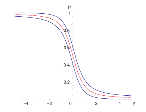
Figure 2:   Dependences of the average probability (dashed line) and the depth of oscillations ($P^{max}$, $P^{min}$ - solid lines) on $y$ for $y_{0}=-5$. The resonance layer corresponds to $y=0$ and the resonance layer is given by the interval $y=-1\div 1$. For $\tan^{2}\theta=0.4$ (large mixing MSW solution) the evolution stops at $y_{f}=0.47$.

The probability is the oscillatory function which is inscribed into the band shown by the solid lines. There is no explicit dependence on the vacuum angle $\theta$. With decrease of $y_{0}$, the oscillation band becomes narrower approaching the line of non-oscillatory conversion. For zero final density: $y_{f}=1/\tan 2\theta.$ The smaller the mixing (and therefore, the larger final $y_{f}$) the stronger transition.

3. Adiabaticity violation.  If density changes rapidly, so that the condition (9) is not satisfied, the transitions $\nu_{1m}\leftrightarrow\nu_{2m}$ become efficient  [6, 12]. Therefore admixtures of the eigenstates in a given propagating state change: $\theta_{a}=\theta_{a}(x)$. Now all three degrees of freedom - phase, flavor, and admixture - become operative. Typically, adiabaticity breaking leads to weakening of the flavor transition and enhancement of oscillations.

4. Graphic representation  [13] is based on

Figure 3: Graphic representation of the MSW effect. The direction of the cone axis is determined by $2\theta_{m}$, the cone angle is given by $\theta_{a}$ and the position of the neutrino vector on the surface of the cone is fixed by the phase $\Phi_{m}$. In the adiabatic case (left panel) the direction of the axis flips according to $\theta_{m}{n_{e}}$ change, and the cone angle is unchanged. In the non-adiabatic case (right panel) also the cone angle changes.

the analogy of the neutrino evolution with the behavior of spin of the electron in the magnetic field. The neutrino evolution equation can be written as

$$\frac{d\vec{\nu}}{dt}=\left(\vec{B}\times\vec{\nu}\right)~{},$$ (12)

where the neutrino vector of length 1/2 (equivalent of spin) is

$$\vec{\nu}\equiv(R,I,P-1/2)=\left({\rm Re}\nu_{e}^{\dagger}\nu_{\mu},~{}~{}{\rm Im}\nu_{e}^{\dagger}\nu_{\mu},~{}~{}\nu_{e}^{\dagger}\nu_{e}-1/2\right),$$ (13)

$\nu_{\alpha}=\nu_{\alpha}(x)$, ($\alpha=\mu,e$) are the neutrino wave functions, and $P$ is the survival probability . The vector of “magnetic field” equals

$$\vec{B}\equiv\frac{2\pi}{l_{m}}(\sin 2\theta_{m},~{}~{}0,~{}~{}\cos 2\theta_{m})~{},$$ (14)

where $l_{m}=2\pi/\Delta H$ is the oscillation length in matter. The vector $\vec{\nu}$ moves on the surface of the cone with axis $\vec{B}$ according to increase of the oscillation phase, $\Phi_{m}$.

3 Realizations of the MSW effect

General conditions for the MSW conversion are: (i) slow enough density change; (ii) crossing the resonance layer; (iii) large enough matter width (minimal width condition) [14]. These conditions are satisfied for the solar neutrinos inside the Sun, for supernova neutrinos inside collapsing stars and can be satisfied for neutrinos in the Early Universe.

3.1 Solar Neutrinos. Large Angle MSW solution

The large mixing MSW conversion provides the solution of the solar neutrino problem [15]. The best fit values of the oscillation parameters from combined analysis of the solar and KamLAND data (in assumption of the CPT invariance) are [16]:

$$\Delta m^{2}=7.9\cdot 10^{-5}~{}{\rm eV}^{2},~{}~{}~{}~{}\tan^{2}\theta=0.40.$$ (15)

Analysis of the solar neutrino data alone leads to smaller mass split, $\Delta m^{2}=6.3\cdot 10^{-5}{\rm eV}^{2}$ which agrees with (15) within $1\sigma$.

1. Physical picture.  According to LMA, inside the Sun the initially produced electron neutrinos undergo the highly adiabatic conversion: $\nu_{e}\rightarrow\cos\theta_{m}^{0}\nu_{1}+\sin\theta_{m}^{0}\nu_{2}$, where $\theta_{m}^{0}$ is the mixing angle in the production point. On the way from the central parts of the Sun the coherence of neutrino state is lost after several hundreds oscillation lengths [17], and incoherent fluxes of the mass states $\nu_{1}$ and $\nu_{2}$ arrive at the surface of the Earth. In the matter of the Earth $\nu_{1}$ and $\nu_{2}$ oscillate partially regenerating the $\nu_{e}$-flux. The averaged survival probability can be written as

$$P=\sin^{2}\theta+\cos^{2}\theta_{12}^{m0}\cos 2\theta_{12}-\cos 2\theta_{12}^{m0}f_{reg},$$ (16)

where the first term corresponds to the non-oscillatory transition (dominates at the high energies), the second term is the contribution from the averaged oscillations which increases with decrease of energy, and the third term is the regeneration effect $f_{reg}$. At low energies $P$ reduces to the vacuum oscillation probability with very small matter corrections.

2. Status of LMA.   The solution provides a very good global fit of the solar neutrino data. There is no statistically significant deviation from description given by the standard solar model (SSM) [18] and the LMA solution.

The key observation which testifies for the MSW (matter) effect in the Sun is stronger than 1/2 suppression of the signals at SK and SNO. The $\nu_{e}$-survival probability extracted from the CC/NC ratio at SNO is

$$\langle P_{ee}\rangle=0.31^{+0.12}_{-0.08}~{}~{}~{}~{}(3\sigma),$$ (17)

that is, $\langle P_{ee}\rangle<0.50$ at $5\sigma$, whereas the vacuum $2\nu$ oscillations can produce $\langle P_{ee}\rangle\geq 0.5$.

Observations of two other signatures of the solution (i) the upturn of the spectrum at low energies ($E<7-8$ MeV), (ii) the day-night asymmetry of signals with larger flux during the night are the main objectives of the forthcoming studies.

No viable alternative to the LMA solution exists and possible effects beyond LMA are substantially restricted already now.

There is a very good agreement of the results from solar neutrinos and KamLAND which implies the CPT conservation. Furthermore, it shows correctness of theory of both the vacuum oscillations and conversion in matter.

3. Testing the MSW effect in the Sun.   Important way to test the effect is to introduce the free parameter, $a_{MSW}$, in the the matter potential

$$V\rightarrow a_{MSW}V,$$ (18)

and to determine $a_{MSW}$ from the data [19]. The global analysis of the solar and reactor (KamLAND + CHOOZ) results with $\Delta m_{21}^{2}$, $\sin^{2}\theta_{12}$ and $a_{MSW}$ being unconstrained gives [19] $a_{MSW}=0.8-3.0$ (95% C.L.) with the best fit value $a_{MSW}=1.6$; zero value of $a_{MSW}$ is excluded at $6\sigma$.

4. Precision measurements in solar neutrinos.  Identification of the LMA solution opens new possibilities in [20] (i) precise description of the LMA conversion both inside the Sun and in the Earth taking into account various corrections; (ii) estimation of accuracy of approximation made; (iii) obtaining the accurate analytic expressions for probabilities and observables as functions of the oscillation parameters. There are three small quantities which allow for a very precise expansions.

(1). Smallness of the adiabaticity parameter

$$\gamma(x)=\frac{l_{m}}{4\pi h(x)}\sim 10^{-3}-10^{-4},$$ (19)

where $h$ is the height of solar density profile, allows to use the adiabatic perturbation theory. The non-adiabatic corrections to the averaged survival probability are of the order $\gamma^{2}$ [20].

(2). Smallness of the ratio $\Delta r_{prod}/h$, where $\Delta r_{prod}$ is the size of the neutrino production region, allows one to make the averaging of the survival probability over the neutrino production region in the analytic form [20].

(3). Smallness of the parameter

$$\epsilon(r)=\frac{2EV_{E}}{\Delta m_{12}^{2}}\leq 0.02-0.04,$$ (20)

where $V_{E}$ is the matter potential in the Earth, allows one to develop a very precise perturbation theory for the neutrino oscillations inside the Earth [20].

3.2 MSW effect and Supernova neutrinos

In supernovae one expects new elements of the MSW dynamics. The SN neutrinos probe whole $3\nu$ level crossing scheme, and the effects of both resonances (due to $\Delta m^{2}_{12}$ and $\Delta m^{2}_{13}$) should show up. Various effects associated to the 1-3 mixing can be realized, depending on value of $\theta_{13}$ (fig. 4). As follows from fig. 4, the SN neutrinos are sensitive to $\sin^{2}\theta_{13}$ as small as $10^{-5}$. Studies of the SN neutrinos will also give information on the type of mass hierarchy [21, 22, 23, 24, 25].

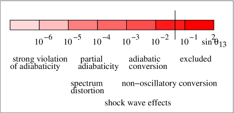
Figure 4: Scales of the 1-3 mixing probed with supernova neutrinos. Indicated are the regions of various effects in neutrino propagation.

1. The small mixing MSW conversion.   This can be realized due to the 1-3 mixing and the “atmospheric” mass split $\Delta m^{2}_{13}$.

2. The non-oscillatory adiabatic conversion  [6] is expected for $\sin^{2}\theta_{13}>10^{-3}$. The density in the production point is extremely large: $n(0)\gg n^{R}$, and therefore the mixing in the initial state is strongly suppressed. So, the neutrino state coincides with the eigenstate in matter: $\nu_{e}=\nu_{2m}$. Due to adiabaticity (no $\nu_{im}\leftrightarrow\nu_{jm}$ transition) the neutrino state coincides with this eigenstate during whole evolution: $\nu(t)=\nu_{2m}$. The interference is negligible since simply there is no second component to interfere with, and consequently, oscillations are absent. The flavor of the neutrino state changes as the flavor of the eigenstate $\nu_{2m}$ and the latter follows the density change.

3. Adiabaticity violation  occurs if the 1-3 mixing is small $\sin^{2}\theta_{13}<10^{-3}$.

The shock wave can reach the region of the neutrino conversion, $\rho\sim 10^{4}$ g/cc, after $t_{s}=(3-5)$ s from the bounce (beginning of the $\nu-$ burst) [26]. Changing suddenly the density profile and therefore breaking the adiabaticity, the shock wave front influences the conversion in the resonance characterized by $\Delta m^{2}_{13}$ and $\sin^{2}\theta_{13}$, if $\sin^{2}\theta_{13}>10^{-4}$.

The following shock wave effects can be seen in neutrinos (antineutrinos) for normal (inverted) hierarchy: (1) change of the total number of events in time [26]; (2) wave of softening of the spectrum which propagates in the energy scale from low energies to high energies [27]; (3) delayed Earth matter effect in the “wrong” channel (e.g., in neutrino channel for normal mass hierarchy) [21]. Modification of the density profile by the shock wave leads to appearance of additional resonances below the front [28]. Reverse shock produces a “double dip” time feature in the average neutrino energy [29, 25]. Monitoring the shock wave with neutrinos can shed some light on the mechanism of explosion.

4. Neutrinos from SN1987A.  After confirmation of the LMA MSW solution we can definitely say that some effect of flavor conversion has already been observed in 1987.

In the case of normal mass hierarchy the adiabatic $\bar{\nu}_{e}\rightarrow\bar{\nu}_{1}$ and $\bar{\nu}_{\mu,\tau}\rightarrow\bar{\nu}_{2}$ transitions occurred inside the star, and then $\nu_{1}$ and $\nu_{2}$ oscillated inside the Earth [10, 21]. In terms of the original fluxes of the electron, and muon antineutrinos, $F^{0}(\bar{\nu}_{e})$ and $F^{0}(\bar{\nu}_{\mu})$, the $\bar{\nu}_{e}-$ flux at the detector can be written as

$$F(\bar{\nu}_{e})=F^{0}(\bar{\nu}_{e})+\bar{p}\Delta F^{0},$$ (21)

where $\Delta F^{0}\equiv F(\bar{\nu}_{\mu})-F(\bar{\nu}_{e})$, and $\bar{p}$ is the permutation factor which can be calculated precisely: $\bar{p}=\sin^{2}\theta_{12}-\bar{f}_{reg}$. Due to difference in the distances traveled by neutrinos to Kamiokande, IMB and Baksan detectors inside the Earth, the $\bar{\nu}_{e}$ regeneration factors $\bar{f}_{reg}$ and therefore $\bar{p}$ differ for these detectors. This can partially explain the difference of the Kamiokande and IMB energy spectra of events [30].

One must take into account the conversion effects in analysis of SN1987A [30] as well as future supernova neutrino data. The conversion can lead to increase of the average energy of the observed events by (30 - 40)%. Inversely, not taking into account the conversion effect produces errors in determination of the average energy of the original $\bar{\nu}_{e}$ spectrum up to 40 - 50 % in Kamiokande, and factor of 2 in IMB.

For the inverted mass hierarchy and $\sin^{2}\theta_{13}>10^{-4}$ one would get nearly complete permutation, $\bar{p}\approx 1$, and therefore a harder $\bar{\nu}_{e}$ spectrum, as well as an absence of the Earth matter effect. This is disfavored by the data [10, 22], see however [23].

4 Matter effects in Neutrino Oscillations

Pure oscillation effect can be realized in the uniform medium. Mixing is constant, $\theta_{m}(E,n)=const$., and therefore

• the flavors of eigenstates do not change;

• the admixtures of eigenstates do not change; there is no $\nu_{1m}\leftrightarrow\nu_{2m}$ transitions: $\nu_{1m}$ and $\nu_{2m}$ are the eigenstates of propagation;

• monotonous increase of $\Phi_{m}$ - the phase difference between the eigenstates occurs.

Only one degree of freedom operates - the phase $\Phi_{m}$ and all others are frozen. This is similar to what happens in vacuum. The depht and length of oscillations are determined by the mixing and energy splitting in matter: $\sin^{2}2\theta_{m}$, $l_{m}=2\pi/(H_{2m}-H_{1m})$.

The oscillations are realized in the Earth which can be considered as the multi-layer medium with nearly constant density in each layer. Variety of possibilities exists depending on the neutrino trajectory (zenith angle), neutrino energy and channel of oscillations.

4.1 Resonance enhancement of oscillations

For a given (constant) density, the length and depth of oscillations depend on the neutrino energy. This leads to a characteristic distortion of the energy spectrum, $F(E)/F_{0}(E)$, where $F_{0}(E)$ and $F(E)$ are, e.g. the spectra of (e.g. $\nu_{e}$) neutrinos in the source and detector correspondingly (fig. 5).

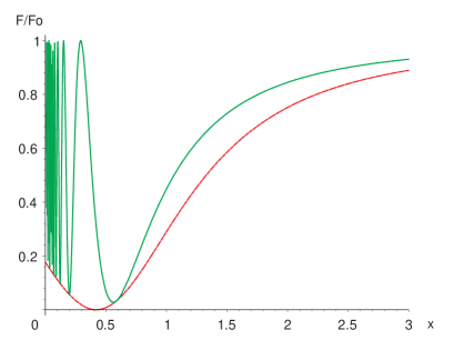
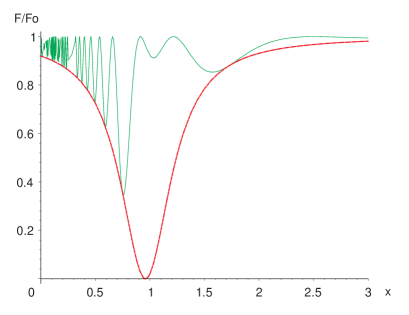
Figure 5:  Resonance enhancement of oscillations in matter with constant density. Shown is the dependence of ratio of the final and original fluxes, (of e.g. $\nu_{e}$) $F/F_{0}$, on energy ($x\equiv l_{\nu}/l_{0}\propto E$) for a thin layer, $L=l_{0}/\pi$, and $\sin^{2}2\theta=0.824$ (left panel), and thick layer, $L=10l_{0}/\pi$, and $\tan^{2}\theta=0.08$ (right panel). The oscillatory curves are inscribed in to the resonance curve $(1-\sin^{2}2\theta_{m})$.

The ratio $F(E)/F_{0}(E)$ given by the survival probability has an oscillatory dependence on the energy. At the resonance energy, $E_{R}$, the oscillations proceed with maximal depth; they are enhanced in the resonance range [6]: $E=E_{R}\pm\Delta E_{R},$ where $\Delta E_{R}=\tan 2\theta E_{R}=\sin 2\theta E_{R}^{0}$ and $E_{R}^{0}=\Delta m^{2}/2\sqrt{2}G_{F}n_{e}$.

The effect is realized for the high energy neutrinos ($E\sim$ GeV) in the mantle of the Earth: constant density is a good first approximation. The effect is expected to be seen in the accelerator long baseline experiments [31], and future high statistics atmospheric neutrino studies [32, 33].

4.2 Parametric enhancement of oscillations

This enhancement is related to certain condition for the phase of oscillations [34, 35]. It provides another way of getting strong transition: no matter enhancement or resonance conversion are needed. No large or maximal mixings in vacuum or matter are required.

The simplest case which can be realized in Nature is neutrinos in the castle wall profile. The latter consists of the alternate layers with two different densities [35, 36, 37]. Let $\Phi_{1}$, $\Phi_{2}$ and $\theta_{1}^{m}$, $\theta_{2}^{m}$ be the phases and mixing angles in the layers 1 and 2.

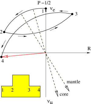
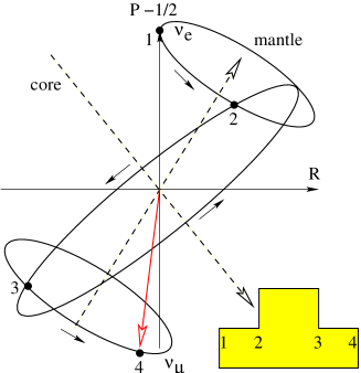
Figure 6: Graphic representation of the parametric enhancement of neutrino oscillations. The notations are explained in fig. 3 and in Eqs. (13, 14). The left panel: the neutrino energy above the resonance energy in the mantle (matter suppressed mixing). The right panel: the neutrino energy is between the core and mantle resonance energies. The mixing in the core is large; in the mantle $\Phi_{1}>\pi/4$ and in the core $\Phi_{2}>2\pi$.

Then under condition:

$$s_{1}c_{2}\cos 2\theta_{1}^{m}+s_{2}c_{1}\cos 2\theta_{2}^{m}=0,$$ (22)

where $s_{1}\equiv\sin\Phi_{i}/2$, $c_{1}\equiv\cos\Phi_{i}/2$, $(i=1,2)$, which is called the parametric resonance condition [38], the flavor transition can be complete. Simple realization of (22) is

$$\Phi_{1}=\Phi_{2}=\pi$$ (23)

which leads to $c_{1}=c_{2}=0$. Eq. (22) can be satisfied for neutrinos (the $\nu_{\mu}-\nu_{e}$ channel with the $\Delta m_{13}^{2}$ and 1-3 mixing) with few GeV energies which cross the core of the Earth [32, 37]. These neutrinos propagate in three layers of matter: mantle-core-mantle. In the approximation of constant densities inside the layers, the profile can be considered as a part of the castle wall profile [36].

For small mixings in both layers, the maximal enhancement occurs when the condition (23) is satisfied (fig.6, left panel). Apparently for few more layers that would lead to maximal transition. On the other hand, even three layers are enough to get nearly maximal transition provided that the mixings in matter are not small (fig. 6, right panel).

For $\Delta m_{13}^{2}=2\cdot 10^{-3}$ eV², the strongest parametric effect (fig. 6 right panel) can be observed in a sample of the atmospheric neutrinos with $E>2.5$ MeV (2 times larger than the energies of multi-GeV sample [32]). Manifestation is the excess of the e-like events for the core crossing trajectories. It can be seen as an enhanced up-down asymmetry of the $e$-like events [32, 33].

4.3 Neutrino oscillations in the low density medium

The condition of low density,

$$V(x)\ll\frac{\Delta m^{2}}{2E},$$ (24)

means that the potential energy is much smaller than the kinetic energy. In this case one can use small parameter $\epsilon(x)$ (20) to develop the perturbation theory [39].

For the LMA oscillation parameters and the solar and supernova neutrinos: $\epsilon(x)=(1-3)\cdot 10^{-2}$. The relevant channel of oscillations is the mass-to-flavor transition, $\nu_{2}\rightarrow\nu_{e}$, since both the solar and SN neutrinos arrive at the Earth as the incoherent fluxes of mass eigenstates. The probability of $\nu_{2}\rightarrow\nu_{e}$ can be written as $P_{2e}=\sin^{2}\theta+f_{reg}$, and oscillations appear in the first order in $\epsilon$. Using the $\epsilon-$ perturbation theory the following expression for the regeneration factor $f_{reg}$ has been obtained [39, 40]

$$f_{reg}=\frac{1}{2}\sin^{2}2\theta\int_{x_{0}}^{x_{f}}dxV(x)\sin\Phi_{m}(x\rightarrow x_{f}).$$ (25)

Here $x_{0}$ and $x_{f}$ are the initial and final points of propagation correspondingly, $\Phi_{m}(x\rightarrow x_{f})$ is the adiabatic phase (2) acquired between a given point of trajectory, $x$, and final point, $x_{f}$. The latter feature has important consequence leading to the attenuation effect.

In the second order in $V$, and therefore $\epsilon$, the regeneration factor becomes [41]

$$f_{reg}=\sin^{2}2\theta\left[\sin\Phi_{m}(x_{c}\rightarrow x_{f})I+\cos 2\theta~{}I^{2}\right],$$ (26)

where for the symmetric profile

$$I=\int_{x_{c}}^{x_{f}}dxV(x)\cos\Phi_{m}(x_{c}\rightarrow x).$$ (27)

In $I$ the integration proceeds from the central point of trajectory, $x_{c}$, to the final point, $x_{f}$. The phase is calculated from $x_{c}$ to a given point $x$. Essentially, the integral $I$ plays the role of expansion parameter and it can be estimated as $I<2EV_{max}/\Delta m^{2}=\epsilon_{max}$.

The perturbation theory [41] can be improved if the expansion is performed with respect to certain potential $V_{0}$ rather than zero. The effective expansion parameter becomes smaller.

4.4 Attenuation effect

Eq. (25) allows one to estimate sensitivity of the oscillation effects to structures of the density profile [39]. Consider some structure in the point $x$ of the trajectory at the distance $d\equiv x_{f}-x$ from the detector. According to (25) for the mass-to-flavor transition the potential $V(x)$ is integrated with $\sin\Phi_{m}(d)$. The larger $d$, (and therefore, the larger $\Phi_{m}(d)$), the stronger averaging effect when some integration over the energy is performed. So, weaker sensitivity of the oscillation effects to remote structures of the profile should show up. The integration over energy with the energy resolution function $R(E,E^{\prime})$,

$$\bar{f}_{reg}(E)=\int dE^{\prime}R(E,E^{\prime})f_{reg}(E^{\prime}),$$ (28)

can be expressed as

$$\bar{f}_{reg}=\frac{1}{2}\sin^{2}2\theta\int_{x_{0}}^{x_{f}}dxV(x)F(x_{f}-x)\sin\Phi_{m}(x\rightarrow x_{f}),$$ (29)

where $F(x_{f}-x)$ is called the attenuation factor [39]. For the box-like function $R(E,E^{\prime})$ with width (energy resolution) $\Delta E$ we obtain

$$F(d)=\frac{1}{z}\sin z,~{}~{}~{}~{}~{}~{}z=\frac{\pi d\Delta E}{l_{\nu}E}.$$ (30)

The factor $F(0)=1$ and it decreases with distance. This means that the contribution of remote structures to the integral (29) is suppressed. The width of the first peak of $F(d)$

$$l_{a}=l_{\nu}\frac{E}{\Delta E}$$ (31)

(corresponds to $z=\pi$) determines the attenuation length: at $d<l_{a}$ the effects of structures are not suppressed. The better the energy resolution, the larger the attenuation length, and consequently, deeper structures can be seen by the neutrino “microscope”. This explains, e.g., why for the solar neutrinos the zenith angle dependence of the Earth mater effect is flat and there is no enhancement of the regeneration for the core crossing trajectories in spite of 2 - 3 times larger density. Indeed, for the solar neutrinos with $E\sim 10$ MeV and $\Delta E/E=0.3$, we obtain $l_{a}=1000$ km and therefore the contribution of the core is attenuated. On the contrary, small structures ($\sim 10$  km) near the surface can produce strong effect. The attenuation length increases with energy. For $E\sim 25$ MeV and $\Delta E/E=0.2$, $l_{a}=4000$ km, so that the core of the Earth can be probed by the SN neutrinos [42].

Another insight into phenomena can be obtained using the adiabatic perturbation theory which leads to [20]

$$f_{reg}=\epsilon(R)\sin^{2}2\theta\sin^{2}[0.5\Phi_{m}(x_{0}\rightarrow x_{f})]+\sin 2\theta Re[c(x_{0}\rightarrow x_{f})].$$ (32)

Here $\epsilon(R)$ is the expansion parameter at the surface of the Earth and

$$c(x)=\int_{x_{0}}^{x}dx^{\prime}\frac{d\theta_{m}(x^{\prime})}{dx^{\prime}}e^{i\Phi_{m}(x^{\prime}\rightarrow x)}$$ (33)

is the amplitude of transition between the eigenstates in matter (the adiabaticity violation effect). In the adiabatic case, $c(x)=0$, the second term in (32) is absent. The adiabaticity condition is broken at the borders of shells only. Due to sharp density change we have for the $j$th border: $d\theta_{m}(x)/dx|_{j}=\Delta V_{j}\delta(x-x_{j})$, where $\Delta V_{j}$ is the jump of the potential between the shells. The integration in $c(x)$ is trivial and simple computations give [20]

$$f_{reg}=\frac{2E\sin^{2}2\theta}{\Delta m^{2}}\sin\frac{\Phi_{0}}{2}\sum_{j=0...n-1}\Delta V_{j}\sin\frac{\Phi_{j}}{2}.$$ (34)

Here $\Phi_{0}$ and $\Phi_{j}$ are the phases acquired along whole trajectory and on the part of the trajectory inside the borders $j$. This formula corresponds to symmetric profile with respect to the center of trajectory. Using (34) one can easily infer the attenuation effect.

5 Conclusions

The large mixing MSW conversion provides the solution of the solar neutrino problem: it leads to determination of $\Delta m_{12}^{2}$ and $\theta_{12}$. Now we have detailed physical picture of the conversion and its very precise analytical description both inside the Sun and in the Earth.

Interesting relation emerges between $\theta_{12}$ determined in the solar neutrinos and the Cabibbo angle: $\theta_{12}+\theta_{C}=\pi/2$. If not accidental, it has important implication for the fundamental physics.

The small mixing MSW conversion driven by the 1-3 mixing can be realized for the supernova neutrinos. Study of these neutrinos will give information on the 1-3 mixing and type of mass hierarchy; it opens unique possibility to perform monitoring of shock wave.

A number of matter effects can be realized for neutrinos propagating inside the Earth: (i) the resonance enhancement of oscillations; (ii) the parametric effects in the multi-layer medium; (iii) the attenuation effect for the low energy neutrinos. The first two effects can be seen in experiments with the atmospheric and accelerator neutrinos. They will play important role in determination of the oscillation parameters and establishing the type of neutrino mass hierarchy. The attenuation effect is realized for the solar and supernova neutrinos, it describes the loss of sensitivity to remote structures of the density profile. The effect is crucial for the oscillation tomography of the Earth.

References

- [1] L. Wolfenstein, Phys. Rev. D17, 2369 (1978); in “Neutrino -78”, Purdue Univ. C3, (1978), Phys. Rev. D20, 2634 (1979).
- [2] B. Pontecorvo, Zh. Eksp. Theor. Fiz. 33 (1957); ibidem 34, 247 (1958).
- [3] Z. Maki, M. Nakagawa and S. Sakata, Prog. Theor. Phys. 28 (1962) 870.
- [4] B. Pontecorvo, ZETF, 53, 1771 (1967) [Sov. Phys. JETP, 26, 984 (1968)]; V. N. Gribov and B. Pontecorvo, Phys. Lett. 28B, 493 (1969).
- [5] V. Barger, K. Whisnant, S. Pakvasa and R.J. N. Phillips, Phys. Rev. D22, 2718 (1980); S. Pakvasa, in DUMAND-80, vol. 2, 457 (1981).
- [6] S. P. Mikheyev and A. Yu. Smirnov, Sov. J. Nucl. Phys. 42, 913 (1985), Nuovo Cim. C9, 17 (1986); S.P. Mikheev and A.Yu. Smirnov, Sov. Phys. JETP 64, 4 (1986).
- [7] P. Langacker, J. P. Leville and J. Sheiman, Phys. Rev. D 27 1228 (1983); V. B. Semikoz, Sov. J. Nucl. Phys. 46, 946 (1987).
- [8] H. Bethe, Phys. Rev. Lett. 56, 1305 (1986).
- [9] A. Messiah, Proc. of the 6th Moriond Workshop on Massive Neutrinos in Particle Physics and Astrophysics, eds O. Fackler and J. Tran Thanh Van, Tignes, France, Jan. 1986, p. 373; S. P. Mikheev and A.Y. Smirnov, Sov. Phys. JETP 65, 230 (1987).
- [10] A. Yu. Smirnov, D. N. Spergel, J. N. Bahcall, Phys. Rev. D49 1389 (1994).
- [11] E. Lisi, A. Marrone, D. Montanino, A. Palazzo and S.T. Petcov, Phys. Rev. D63 093002 (2001); A. Friedland, Phys. Rev. D64, 013008 (2001), and hep-ph/0106042.
- [12] W. C. Haxton, Phys. Rev. Lett. 57, 1271 (1986); S. J. Parke, Phys. Rev. Lett. 57, 1275 (1986); S. P. Rosen and J. M. Gelb, Phys. Rev. D 34, 969 (1986).
- [13] S. P. Mikheyev and A. Yu. Smirnov, Proc. of the 6th Moriond Workshop on massive Neutrinos in Astrophysics and Particle Physics, Tignes, Savoie, France Jan. 1986 (eds. O. Fackler and J. Tran Thanh Van) p. 355 (1986); J. Bouchez et al, Z. Phys. C 32 (1986) 499; V. K. Ermilova, V. A. Tsarev, V. A. Chechin, JETP Lett. 43, 453 (1986).
- [14] C. Lunardini, A. Yu. Smirnov, Nucl. Phys. B583, 260 (2000).
- [15] A. McDonald, these proceedings; Y. Suzuki, these proceedings.
- [16] A. Suzuki, these proceedings, KamLAND Collaboration, K. Eguchi et al., Phys. Rev. Lett., 90, 021802 (2003); T. Araki et al., hep-ex/0406035.
- [17] P. C. de Holanda, A.Yu. Smirnov, Astropart. Phys. 21, 287 (2004).
- [18] J. N. Bahcall, M.H. Pinsonneault, Phys. Rev. Lett. 92, 121301 (2004).
- [19] G. Fogli, E. Lisi, New J. Phys. 6, 139 (2004); G.L. Fogli, E. Lisi, A. Marrone, A Palazzo, Phys. Lett. B583, 149 (2004).
- [20] P. C. de Holanda, Wei Liao, A. Yu. Smirnov, Nucl. Phys. B702, 307 (2004).
- [21] A. S. Dighe, A. Yu. Smirnov, Phys. Rev. D62, 033007 (2000); C. Lunardini, A. Yu. Smirnov, JCAP 0306, 009 (2003).
- [22] H. Minakata, H. Nunokawa, Phys. Lett. B 504, 301 (2001).
- [23] V. Barger, D. Marfatia, B.P. Wood, Phys. Lett. B 532, 19 (2002).
- [24] K. Takahashi, K. Sato, A. Burrows, T. A. Thompson, Phys. Rev. D 68, 113009 (2003).
- [25] G. Raffelt, these proceedings.
- [26] R.C. Schirato and G. M. Fuller, astro-ph/0205390.
- [27] K. Takahashi, K. Sato, H. E. Dalhed, J.R. Wilson, Astropart. Phys. 20, 189 (2003).
- [28] G.L. Fogli, E. Lisi, D. Montanino, A. Mirizzi, Phys. Rev. D 68, 033005 (2003).
- [29] R. Tomas, et al., astro-ph/0407132.
- [30] C. Lunardini, A. Yu. Smirnov, Phys. Rev. D 63, 073009 (2001); Astropart. Phys. 21, 703 (2004); M. L. Costantini, A. Ianni, F. Vissani, Phys. Rev. D 70, 043006 (2004).
- [31] M. Freund, T. Ohlsson, Mod. Phys. Lett. A 15, 867 (2000); M. Freund, M. Lindner, S.T. Petcov, A. Romanino, Nucl. Phys. B 578, 27 (2000); T. Ohlsson, H. Snellman, Phys. Lett. B 474, 153 (2000).
- [32] E. K. Akhmedov, A. Dighe, P. Lipari, A.Y. Smirnov, Nucl. Phys. B 542, 3 (1999).
- [33] J. Bernabeu, S. Palomares-Ruiz, A. Perez, S.T. Petcov, Phys. Lett. B 531, 90 (2002), J. Bernabeu, S. Palomares Ruiz, S.T. Petcov, Nucl. Phys. B 669, 255 (2003).
- [34] V. K. Ermilova, V. A. Tsarev and V. A. Chechin, Kr. Soob, Fiz. [Short Notices of the Lebedev Institute] 5, 26 (1986).
- [35] E. Kh. Akhmedov, Yad. Fiz. 47, 475 (1988) [Sov. J. Nucl. Phys. 47, 301 (1988)].
- [36] Q. Y. Liu, A. Yu. Smirnov, Nucl. Phys. B 524, 505 (1998); Q. Y. Liu, S. P. Mikheyev, A. Yu. Smirnov, Phys. Lett. B440, 319 (1998).
- [37] S. T. Petcov, Phys. Lett. B434 (1998) 321; M. Chizhov, M. Maris, S.T. Petcov, hep-ph/9810501; M.V. Chizhov, S.T. Petcov, Phys. Rev. Lett. 83, 1096 (1999); Phys. Rev. D 63, 073003 (2001).
- [38] E.K. Akhmedov, Nucl. Phys. B 538, 25 (1999), [hep-ph/9805272]; hep-ph/9903302; Pramana 54, 47 (2000), [hep-ph/9907435]. E.K. Akhmedov, A.Yu. Smirnov, Phys. Rev. Lett. 85, 3978 (2000), and hep-ph/9910433.
- [39] A. N. Ioannisian, A.Yu. Smirnov, Phys. Rev. Lett. 93, 241801 (2004).
- [40] E. Kh. Akhmedov, M.A. Tortola, J.W.F. Valle, JHEP 0405, 057 (2004).
- [41] A. N. Ioannisian, N.A. Kazarian, A.Yu. Smirnov, D. Wyler, hep-ph/0407138.
- [42] M. Lindner, T. Ohlsson, R. Tomas, W. Winter, Astropart. Phys. 19, 755 (2003).