A semi-analytic calculation on the atmospheric tau neutrino flux in the GeV to TeV energy range

Abstract

We present a semi-analytic calculation on the atmospheric tau neutrino flux in the GeV to TeV energy range. The atmospheric $\nu_{\tau}$ flux is calculated for the entire zenith angle range. This flux is contributed by the oscillations of muon neutrinos coming from the two-body $\pi,\ K$ decays and the three-body $\mu^{\pm}$ decays, and the intrinsic tau neutrino flux surviving the oscillations. The uncertainties in our calculations are discussed in detail. The implications of our result are also discussed.

I Introduction

The flux of atmospheric tau neutrinos in the GeV to TeV energy range comes from both the intrinsic atmospheric $\nu_{\tau}$ flux and the flux due to the neutrino flavor oscillation $\nu_{\mu}\to\nu_{\tau}$. The importance of understanding such a flux is twofold. First, the detection of atmospheric $\nu_{\tau}$ flux is important for confirming the atmospheric $\nu_{\mu}\to\nu_{\tau}$ oscillation scenario which is so far established only by the $\nu_{\mu}$ disappearance measurement Ashie:2004mr . Second, the atmospheric $\nu_{\tau}$ flux is also an important background for the search of astrophysical $\nu_{\tau}$ fluxes Athar:2004pb ; Athar:2004uk or exotic $\nu_{\tau}$ fluxes such as those arising from dark matter annihilations Bertone:2004pz , if an effective tau neutrino astronomy can be developed in the future. The techniques for identifying the tau neutrinos in the GeV to TeV energy range are discussed both in the experiments for atmospheric tau neutrinos Stanev:1999ki and in the accelerator-based neutrino experiments Zalewska:2004nd ; Campagne:2004ay . Due to growing attentions on the direct $\nu_{\tau}$ detections, it is important to investigate closely the flux of atmospheric tau neutrinos in such an energy range.

The calculation of atmospheric $\nu_{\mu}$ and $\nu_{e}$ fluxes has reached to a rather advanced stage Gaisser:2002jj . The upward atmospheric $\nu_{\tau}$ flux can be calculated easily from the above $\nu_{\mu}$ flux by multiplying the $\nu_{\mu}\to\nu_{\tau}$ oscillation probability arising from neutrino propagation inside the Earth. In such a case, the $\nu_{\mu}\to\nu_{\tau}$ oscillations in the atmosphere is generally negligible. However, the atmospheric neutrino coming with a zenith angle $\xi$ less than $90^{\circ}$ directly arrives at the detector. Hence oscillations of these neutrinos in the atmosphere are precisely the problems one has to deal with. In this regard, an estimation of the atmospheric $\nu_{\tau}$ flux is given in Ref. Athar:2004pb for the two-flavor neutrino oscillation framework Athar:2004mm . A detailed calculation of this flux in the same neutrino oscillation framework is given in Athar:2004um for zenith angles $0\leq\xi\leq 60^{\circ}$, where the Earth curvature can be neglected in the calculation. The extension of such a calculation to large zenith angles is important. First of all, the path-length for the neutrino propagation in the atmosphere increases drastically from $\xi=60^{\circ}$ to $\xi=90^{\circ}$. As a result, the atmospheric $\nu_{\tau}$ flux also increases drastically in this zenith angle range by the enhanced $\nu_{\mu}\to\nu_{\tau}$ oscillation probabilities. Secondly, the calculation of upward atmospheric $\nu_{\tau}$ flux is also important since most of the neutrino telescopes aim at detecting upward neutrino fluxes. In this paper, we shall extend the calculation in Athar:2004um to the entire zenith angle range.

The calculations of atmospheric $\nu_{\tau}$ flux for zenith angles $60^{\circ}\leq\xi\leq 90^{\circ}$ and zenith angles slightly larger than $90^{\circ}$ are much more involved as we shall discuss later. Besides extending our previous calculation to the entire zenith angles, we also extend its validity from the energy range $E_{\nu}\geq 10$ GeV to the energy range $E_{\nu}\geq 1$ GeV. This improvement is accomplished by including the muon-decay contribution $\mu^{+}\to\bar{\nu}_{\mu}\nu_{e}e^{+}$ and $\mu^{-}\to\nu_{\mu}\bar{\nu}_{e}e^{-}$ to the intrinsic atmospheric $\nu_{\mu}$ flux, in additional to those arising from two-body $\pi$ and $K$ decays. Such a contribution also generates $\nu_{\tau}$ flux by $\nu_{\mu}\to\nu_{\tau}$ oscillations. This part of $\nu_{\tau}$ flux is non-negligible for $E_{\nu}\leq 10$ GeV. Furthermore, it contributes to the total $\nu_{\tau}$ flux in a growing percentage as the zenith angle $\xi$ increases.

The paper is organized as follows. In Sec. II, we introduce the method for calculating the intrinsic muon and tau neutrino fluxes. Particularly we outline the strategy for dealing with atmospheric neutrino flux for $\xi>60^{\circ}$. In Sec. III, we present the atmospheric tau neutrino flux taking into account the neutrino flavor oscillations. We discuss implications of our results in Sec. IV.

II The Intrinsic Atmospheric Neutrino Fluxes

II.1 Intrinsic atmospheric muon neutrino flux

We follow the approach in Gaisser:2001sd for computing the flux of intrinsic atmospheric muon neutrinos which could oscillate into tau neutrinos. This approach computes the flux of muon neutrinos coming from pion and kaon decays. The method for computing muon neutrinos arising from muon decays will be discussed later. The $\nu_{\mu}$ flux arising from $\pi$ decays reads:

$$\frac{\mbox{d}^{2}N^{\pi}_{\nu_{\mu}}(E,\xi,X)}{\mbox{d}E\mbox{d}X} = \int_{E}^{\infty}\mbox{d}E_{N}\int_{E}^{E_{N}}\mbox{d}E_{\pi}\frac{\Theta(E_{\pi}-\frac{E}{1-r_{\pi}})}{d_{\pi}E_{\pi}(1-r_{\pi})}\int_{0}^{X}\frac{\mbox{d}X^{\prime}}{\lambda_{N}}P_{\pi}(E_{\pi},X,X^{\prime})$$ (1)

$$\times\frac{1}{E_{\pi}}F_{N\pi}(E_{\pi},E_{N})\times\exp\left(-\frac{X^{\prime}}{\Lambda_{N}}\right)\phi_{N}(E_{N}),$$

where $E$ is the neutrino energy, $\xi$ is the zenith angle in the direction of incident cosmic-ray nucleons, $r_{\pi}=m_{\mu}^{2}/m_{\pi}^{2}$, $d_{\pi}$ is the pion decay length in units of g/cm², $\lambda_{N}$ is the nucleon interaction length while $\Lambda_{N}$ is the corresponding nucleon attenuation length, and $\phi_{N}(E_{N})$ is the primary cosmic-ray spectrum. For the simplicity in discussions, we only consider the proton component of $\phi_{N}$, which is given by Gaisser:2002jj

$$\phi_{p}(E_{p})=1.49\cdot\left(E_{p}+2.15\cdot\exp(-0.21\sqrt{E_{p}})\right)^{-2.74},$$ (2)

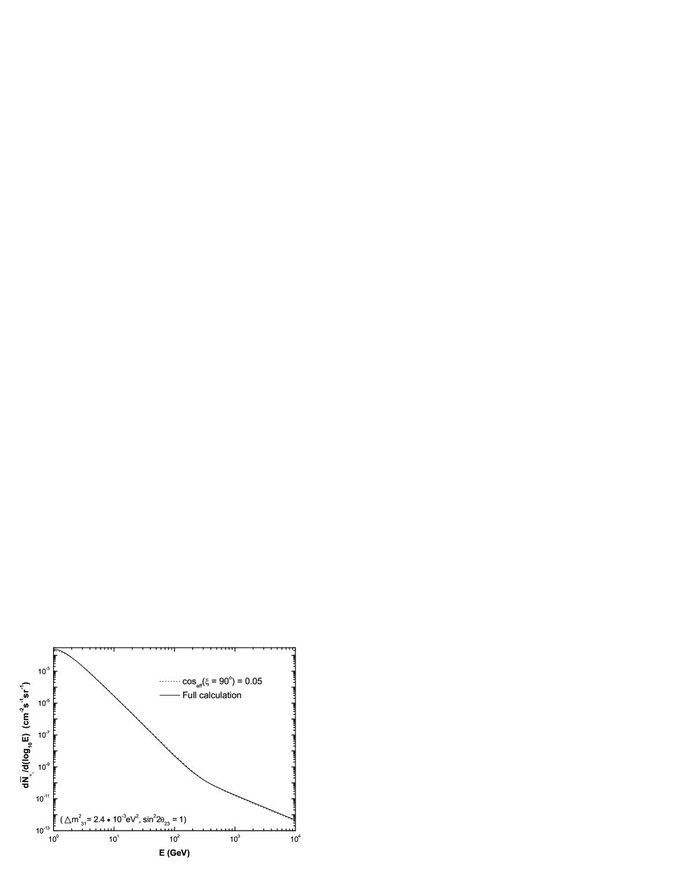
Figure 7: The comparison of atmospheric $\nu_{\tau}$ flux obtained by using $\cos_{\rm eff}\xi$ and that obtained by the full calculation for $\xi=90^{\circ}$.

in units of cm^-2s^-1sr^-1GeV^-1. Since our concerned energy range for the primary cosmic ray flux is between $10^{1}$ GeV and $10^{5}$ GeV per nucleon (corresponding to roughly a neutrino energy range between $10^{0}$ GeV and $10^{4}$ GeV), the contribution by the heavier nuclei on the neutrino flux is between $25\%$ and $40\%$ according to Fig. 7 of Ref. Gaisser:2002jj . Hence one expects the eventual atmospheric $\nu_{\tau}$ flux is underestimated by $25\%$ to $40\%$ by considering only the proton component of the primary cosmic ray flux. The function $P_{\pi}(E_{\pi},X,X^{\prime})$ is the probability that a charged pion produced at the slant depth $X^{\prime}$ (g/cm²) survives to the depth $X$ ($>X^{\prime}$), $F_{N\pi}(E_{\pi},E_{N})$ is the normalized inclusive cross section for $N+{\rm air}\to\pi^{\pm}+Y$ given by Gaisser:2001sd :

$$F_{N\pi}(E_{\pi},E_{N})\equiv\frac{E_{\pi}}{\sigma_{N}}\frac{{\mbox{d}}\sigma(E_{\pi},E_{N})}{{\mbox{d}}E_{\pi}}=c_{+}(1-x)^{p_{+}}+c_{-}(1-x)^{p_{-}},$$ (3)

where $x=E_{\pi}/E_{N}$, $c_{+}=0.92$, $c_{-}=0.81$, $p_{+}=4.1$, and $p_{-}=4.8$. We remark that $c_{+}(1-x)^{p_{+}}$ corresponds to the $\pi^{+}$ production while $c_{-}(1-x)^{p_{-}}$ corresponds to the $\pi^{-}$ production. The kaon contribution to the atmospheric $\nu_{\mu}$ flux has the same form as Eq. (1) with an inclusion of the branching ratio $B(K\to\mu\nu)=0.635$ and appropriate replacements in kinematic factors and the normalized inclusive cross section. In particular, $F_{NK}(E_{K},E_{N})$ can be parameterized as Eq. (3) with $c_{+}=0.037$, $c_{-}=0.045$, $p_{+}=0.87$, and $p_{-}=3.5$. Finally the nucleon interaction length, $\lambda_{N}$, and the nucleon attenuation length, $\Lambda_{N}$, are both model dependent. A simplified approach based upon the Feynman scaling render both $\lambda_{N}$ and $\Lambda_{N}$ energy independent and $Z_{pp}\equiv 1-\lambda_{p}/\Lambda_{p}=0.263$ COSMIC ; Lipari:1993hd , whereas a PYTHIA pythia calculation give rise to an energy dependent $Z_{pp}$ Gondolo:1995fq . Both results on $Z_{pp}$ are compared in Fig. 1 where we have extrapolated the energy dependent $Z_{pp}(E)$ in Ref. Gondolo:1995fq down to $E=1$ GeV. The above two approaches for calculating the hadronic $Z$ moments also give rise to different results for $Z_{\pi\pi}$, $Z_{KK}$, $Z_{N\pi}$ and $Z_{NK}$, where the last two $Z$-moments are related to the productions of pions and kaons by the nucleon-air collisions. In this paper, we shall only study the $Z_{pp}$ dependence of the atmospheric $\nu_{\mu}$ flux (and consequently the atmospheric $\nu_{\tau}$ flux) since the dependencies of this flux on $Z_{N\pi}$ and $Z_{NK}$ have been studied in Agrawal:1995gk . Furthermore, compared to the $Z_{pp}$ case, the values of $Z_{\pi\pi}$ and $Z_{KK}$ obtained by the Feynman scaling do not differ significantly from those obtained by the PYTHIA calculations, as seen from Gondolo:1995fq .

To proceed for calculating $\mbox{d}^{2}N^{\pi}_{\nu_{\mu}}(E,\xi,X)/\mbox{d}E\mbox{d}X$, we note that $P_{\pi}(E_{\pi},X,X^{\prime})$ is given by Lipari:1993hd

$$P_{\pi}(E_{\pi},X,X^{\prime})=\exp\left(-\frac{X-X^{\prime}}{\Lambda_{\pi}}\right)\cdot\exp\left(-\frac{m_{\pi}c}{\tau_{\pi}}\int_{X^{\prime}}^{X}\frac{{\mbox{d}}T}{\rho(T)}\right),$$ (4)

where $\Lambda_{\pi}=160$ g/cm² is the pion attenuation constant, $\tau_{\pi}$ is the pion lifetime at its rest frame, while $\rho(T)$ is the atmosphere mass density at the slant depth $T$. For $\xi\leq 60^{\circ}$, the curvature of the Earth can be neglected so that $\rho(T)=T\cos\xi/h_{0}$ with $h_{0}=6.4$ km the scale height for an exponential atmosphere. In this approximation, the above survival probability can be written as Gaisser:2001sd

$$P_{\pi}(E_{\pi},X,X^{\prime})=\exp\left(-\frac{X-X^{\prime}}{\Lambda_{\pi}}\right)\cdot\left(\frac{X^{\prime}}{X}\right)^{\epsilon_{\pi}/E_{\pi}\cos\xi},$$ (5)

where $\epsilon_{\pi}=m_{\pi}c^{2}h_{0}/c\tau_{\pi}$ is the pion decay constant. Depending on the zenith angle, we apply either Eq. (4) or Eq. (5) to perform the calculations. The kaon survival probability $P_{K}(E_{K},X,X^{\prime})$ has the same form as $P_{\pi}(E_{\pi},X,X^{\prime})$ except replacing $\Lambda_{\pi}$ with $\Lambda_{K}$ and $\epsilon_{\pi}$ with $\epsilon_{K}$. The two-body decay contribution to the atmospheric $\nu_{\mu}$ flux is given by the sum of $\mbox{d}^{2}N^{\pi}_{\nu_{\mu}}(E,\xi,X)/\mbox{d}E\mbox{d}X$ and $\mbox{d}^{2}N^{K}_{\nu_{\mu}}(E,\xi,X)/\mbox{d}E\mbox{d}X$.

We recall that Eq. (1) and its corresponding form in the kaon decay case only calculate the flux of muon neutrinos arising from two-body pion and kaon decays. To calculate the contribution from three-body muon decays, it is useful to first obtain the muon flux Gaisser:2001sd :

$$\frac{\mbox{d}N^{\pi}_{\mu}(E,\xi,X)}{\mbox{d}E} = \int_{E^{\prime}}^{\infty}\mbox{d}E_{N}\int_{E^{\prime}}^{E_{N}}\mbox{d}E_{\pi}\int_{0}^{X}{\mbox{d}}X^{{}^{\prime\prime}}P_{\mu}(E,X,X^{{}^{\prime\prime}})$$ (6)

$$\times \frac{\Theta(E_{\pi}-E^{\prime})\Theta(\frac{E^{\prime}}{r_{\pi}}-E_{\pi})}{d_{\pi}E_{\pi}(1-r_{\pi})}\times\int_{0}^{X^{{}^{\prime\prime}}}\frac{\mbox{d}X^{\prime}}{\lambda_{N}}P_{\pi}(E_{\pi},X^{{}^{\prime\prime}},X^{\prime})$$

$$\times \frac{1}{E_{\pi}}F_{N\pi}(E_{\pi},E_{N})\times\exp\left(-\frac{X^{\prime}}{\Lambda_{N}}\right)\phi_{N}(E_{N}),$$

where $E^{\prime}$ and $E$ are muon energies at slant depths $X^{{}^{\prime\prime}}$ and $X$ respectively, while $P_{\mu}(E,X,X^{{}^{\prime\prime}})$ is the muon survival probability given by Lipari:1993hd

$$P_{\mu}(E,X,X^{{}^{\prime\prime}})=\exp\left[-\frac{m_{\mu}c}{\tau_{\mu}}\int_{X^{{}^{\prime\prime}}}^{X}{\mbox{d}}T\frac{1}{E(T-X^{{}^{\prime\prime}},E^{\prime})\rho(T)}\right],$$ (7)

where $\tau_{\mu}$ is the muon lifetime at its rest frame and $E(T-X^{{}^{\prime\prime}},E^{\prime})$ is the muon energy at the slant depth $T$ with $E^{\prime}$ the muon energy at its production point $X^{{}^{\prime\prime}}$. For the zenith angle $\xi\leq 60^{\circ}$, the above survival probability can be written as Gaisser:2001sd

$$P_{\mu}(E,X,X^{{}^{\prime\prime}})=\left(\frac{X^{{}^{\prime\prime}}}{X}\frac{E}{E+\alpha(X-X^{{}^{\prime\prime}})}\right)^{\epsilon_{\mu}/(E\cos\xi+\alpha X\cos\xi)},$$ (8)

with $\epsilon_{\mu}=m_{\mu}c^{2}h_{0}/c\tau_{\mu}$ the muon decay constant and $\alpha\approx 2$ MeV/g/cm² characterizing the muon ionization loss in the medium Rossi . Since the muons are polarized, it is convenient to keep track of the right-handed and left-handed muon fluxes separately. The probability for a produced $\mu^{-}$ to be right-handed or left-handed is determined by the muon polarization Barr:1988rb ; Barr:1989ru :

$$P_{\mu}(x)=\frac{1+r_{\pi}}{1-r_{\pi}}-\frac{2r_{\pi}}{(1-r_{\pi})x},$$ (9)

with $x=E_{\mu}/E_{\pi}$ and $r_{\pi}=m_{\mu}^{2}/m_{\pi}^{2}$. Hence $P_{R,L}(x)=\frac{1}{2}\left(1\pm P_{\mu}(x)\right)$ are the probabilities for the produced muon to be right-handed or left-handed respectively. The polarization for $\mu^{+}$ has an opposite sign to that of $\mu^{-}$. The probabilities $P_{R,L}(x)$ should be inserted into Eq. (6) for obtaining four different components of the muon flux: $\mbox{d}N^{\pi}_{\mu^{+}_{R}}/\mbox{d}E$, $\mbox{d}N^{\pi}_{\mu^{-}_{R}}/\mbox{d}E$, $\mbox{d}N^{\pi}_{\mu^{+}_{L}}/\mbox{d}E$, and $\mbox{d}N^{\pi}_{\mu^{-}_{L}}/\mbox{d}E$. There are additional four components of the muon flux arising from the kaon decays. The calculation of these components proceeds in the same way as the pion decay case. The $\nu_{\mu}$ flux resulting from the muon flux is then given by Lipari:1993hd

$$\frac{\mbox{d}^{2}N^{\mu^{\pm}}_{\nu_{\mu}}(E,\xi,X)}{\mbox{d}E\mbox{d}X}=\sum_{s=L,R}\int_{E}^{\infty}{\mbox{d}}E_{\mu}\frac{F_{\mu^{\pm}_{s}\to\nu_{\mu}}(E/E_{\mu})}{d_{\mu}(E_{\mu},X)E_{\mu}}\cdot\frac{\mbox{d}N_{\mu_{s}^{\pm}}(E_{\mu},\xi,X)}{\mbox{d}E_{\mu}},$$ (10)

where $d_{\mu}(E_{\mu},X)$ is the muon decay length in units of g/cm² at the slant depth $X$ and $F_{\mu^{\pm}_{s}\to\nu_{\mu}}(E/E_{\mu})$ is the decay distribution of $\mu^{\pm}_{s}\to\nu_{\mu}$. Precisely, in the ultra-relativistic limit, one has Lipari:1993hd

$$F_{\mu^{-}\to\nu_{\mu}}(y)=g_{0}(y)+P_{\mu}g_{1}(y),$$ (11)

with $g_{0}(y)=5/3-3y^{2}+4y^{3}/3$, $g_{1}(y)=1/3-3y^{2}+8y^{3}/3$. We do not include the charm-hadron decay contribution to the muon neutrino flux. It is shown in Ref. Athar:2004um that charm-hadron decays contribute less than $5\%$ to the overall muon neutrino flux for $E_{\nu}<10^{5}$ GeV.

II.2 Intrinsic atmospheric tau neutrino flux

To completely determine the atmospheric tau neutrino flux, we also need to calculate its intrinsic component. Since the flux of intrinsic atmospheric $\nu_{\tau}$ arises from $D_{s}$ decays, one calculates this flux by solving the following cascade equations COSMIC :

$$\frac{{\mbox{d}}\phi_{p}(E,X)}{{\mbox{d}}X} = -\frac{\phi_{p}}{\lambda_{p}}+Z_{pp}\frac{\phi_{p}}{\lambda_{p}}$$

$$\frac{{\mbox{d}}\phi_{D_{s}}(E,X)}{{\mbox{d}}X} = -\frac{\phi_{D_{s}}}{\lambda_{D_{s}}}-\frac{\phi_{D_{s}}}{d_{D_{s}}}+Z_{pD_{s}}\frac{\phi_{p}}{\lambda_{p}}+Z_{D_{s}D_{s}}\frac{\phi_{D_{s}}}{\lambda_{D_{s}}}$$

$$\frac{{\mbox{d}}\phi_{\nu_{\tau}}(E,X)}{{\mbox{d}}X} = Z_{D_{s}\nu_{\tau}}\frac{\phi_{D_{s}}}{d_{D_{s}}},$$ (12)

where the particle flux ${\mbox{d}}\phi_{i}(E,X)/{\mbox{d}}X$ denotes ${\mbox{d}}^{2}N_{i}(E,X)/{\mbox{d}}E{\mbox{d}}X$, $d_{i}$ and $\lambda_{i}$ denote particle’s decay and interaction length in g/cm² respectively, and the $Z$ moments $Z_{ij}$ are defined by

$$Z_{ij}(E_{j})\equiv\int_{E_{j}}^{\infty}{\mbox{d}}E_{i}\frac{\phi_{i}(E_{i})}{\phi_{i}(E_{j})}\frac{\lambda_{i}(E_{j})}{\lambda_{i}(E_{i})}\frac{{\mbox{d}}n_{iA\to jY}(E_{i},E_{j})}{{\mbox{d}}E_{j}},$$ (13)

with ${\mbox{d}}n_{iA\to jY}(E_{i},E_{j})\equiv{\mbox{d}}\sigma_{iA\to jY}(E_{i},E_{j})/\sigma_{iA}(E_{i})$. In the decay process, the scattering length $\lambda_{i}$ is replaced by the decay length $d_{i}$ while ${\mbox{d}}n_{iA\to jY}(E_{i},E_{j})/{\mbox{d}}E_{j}$ is replaced by the decay distribution $F_{i\to j}(E_{j}/E_{i})$. In our concerned energy range, the chain of equations in (12) can be easily solved by simplifying the second equation, namely by neglecting terms $\phi_{D_{s}}/\lambda_{D_{s}}$ and $Z_{D_{s}D_{s}}\phi_{D_{s}}/\lambda_{D_{s}}$. One obtains

$$\frac{\mbox{d}^{2}N_{\nu_{\tau}}(E,X)}{\mbox{d}E\mbox{d}X}=\frac{Z_{pD_{s}}(E)Z_{D_{s}\nu_{\tau}}(E)}{1-Z_{pp}(E)}\cdot\frac{\exp(-X/\Lambda_{p})\phi_{p}(E)}{\Lambda_{p}}.$$ (14)

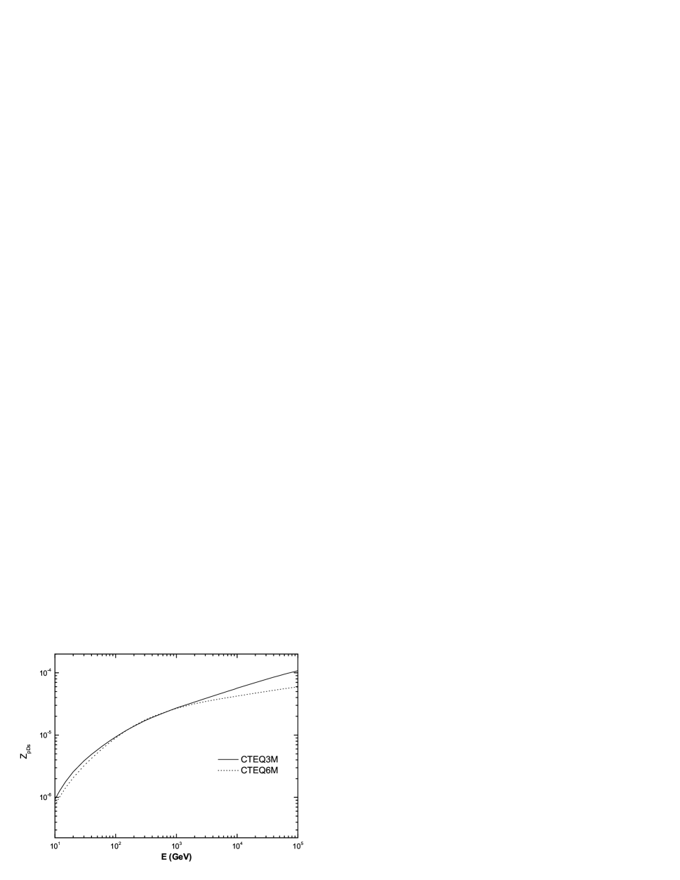
Figure 2: The $Z$ moment $Z_{pD_{s}}$ obtained by perturbative QCD with CTEQ3 and CTEQ6 parton distribution functions respectively.

We use two different values for $Z_{pp}\equiv 1-\lambda_{p}/\Lambda_{p}$ as shown in Fig. 1. To determine $Z_{pD_{s}}$, it is necessary to calculate ${\mbox{d}}\sigma_{pA\to D_{s}Y}(E_{p},E_{D_{s}})/{\mbox{d}}E_{D_{s}}$. Since $D_{s}$ meson is heavy enough, the above differential cross section is calculable using perturbative QCD Pasquali:1998xf . In this work, the next-to-leading order (NLO) perturbative QCD Nason:1989zy ; Mangano:1991jk with CTEQ6 parton distribution functions Pumplin:2002vw are employed to calculate the differential cross section of $pA\to c\bar{c}$. To obtain ${\mbox{d}}\sigma_{pA\to D_{s}Y}(E_{p},E_{D_{s}})/{\mbox{d}}E_{D_{s}}$, we multiply the charm quark differential cross section by the probability factor $13\%$ to account for the fragmentation process $c\to D_{s}$ Pasquali:1998xf . In Fig. 2, we compare our $Z_{pD_{s}}$ to a previous result obtained by the CTEQ3 parton distribution functions Pasquali:1998ji . In the latter work, the NLO pertubative QCD effects are taken into account by the $K$ factor defined by

$$K(E,x_{E})=\frac{\mbox{d}\sigma^{\rm NLO}(E,x_{E})/{\mbox{d}x_{E}}}{\mbox{d}\sigma^{\rm LO}(E,x_{E})/{\mbox{d}x_{E}}},$$ (15)

where $\mbox{d}\sigma^{\rm LO}(E,x_{E})/{\mbox{d}x_{E}}$ and $\mbox{d}\sigma^{\rm NLO}(E,x_{E})/{\mbox{d}x_{E}}$ are leading order and next-to-leading order differential cross sections for $pA\to c\bar{c}$ respectively, with $x_{E}=E_{c}/E_{p}$. For QCD renormalization scale $\mu=m_{c}$ and the factorization scale $M=2m_{c}$, the $K$ factor is fitted to be Pasquali:1998ji

$$K(E,x_{E}) = 1.36+0.42\ln\left(\ln(E/{\rm GeV})\right)$$ (16)

$$+ \left(3.40+18.7(E/{\rm GeV})^{-0.43}-0.079\ln(E/{\rm GeV})\right)x_{E}^{1.5}.$$

We apply this $K$ factor to our calculation with CTEQ6 parton distribution functions. Comparing this result with that obtained by applying CTEQ3 parton distribution functions, one acquires an idea on the uncertainty of perturbative QCD approach to the charm hadron production cross section. It is seen from Fig. 2 that both $Z$ moments agree well for energies below TeV. For $E=10$ TeV, they differ by about $30\%$.

Besides perturbative QCD approach, there are non-perturbative approach for computing the charm hadron production cross section. In fact, such non-perturbative approaches Kaidalov:1985jg ; Bugaev:1998bi are motivated to accommodate accelerator data on strange particle productions, which are underestimated by the perturbative QCD approach. It is desirable to apply these approaches to charm hadron productions. The quark-gluon-string-model (QGSM) Kaidalov:1985jg is a non-perturbative approach based upon the string fragmentation, where the model parameters are tuned to the production cross section of strange particles. The recombination-quark-parton-model (RQPM) Bugaev:1998bi is also a phenomenological approach which takes into account the contribution of the intrinsic charm in the nucleon to the charm hadron production cross section. Detailed comparisons of these two models with perturbative QCD approach on the charm hadron productions are given in Costa:2000jw . It is shown that perturbative QCD approach gives the smallest charm production $Z$ moments. It is clear that the model dependencies on the charm hadron productions affect both the prompt atmospheric muon neutrino flux and the intrinsic atmospheric tau neutrino flux. A detailed study on the model dependencies of the intrinsic atmospheric tau neutrino flux is given in Costa:2001fb . We shall further discuss these model dependencies after commenting on the $Z$ moment $Z_{D_{s}\nu_{\tau}}$.

We note that $Z_{D_{s}\nu_{\tau}}$ is related to the energy distributions of the $D_{s}$ decays into tau neutrinos. One arises from the decay $D_{s}\to\nu_{\tau}\tau$, and the other follows from the subsequent tau-lepton decay, $\tau\to\nu_{\tau}+X$. The latter contribution is calculated using the decay distributions of the decay modes $\tau\to\nu_{\tau}\rho$, $\tau\to\nu_{\tau}\pi$, $\tau\to\nu_{\tau}a_{1}$ Li:1995aw ; Pasquali:1998xf , and $\tau\to\nu_{\tau}l\nu_{l}$ COSMIC ; Lipari:1993hd .

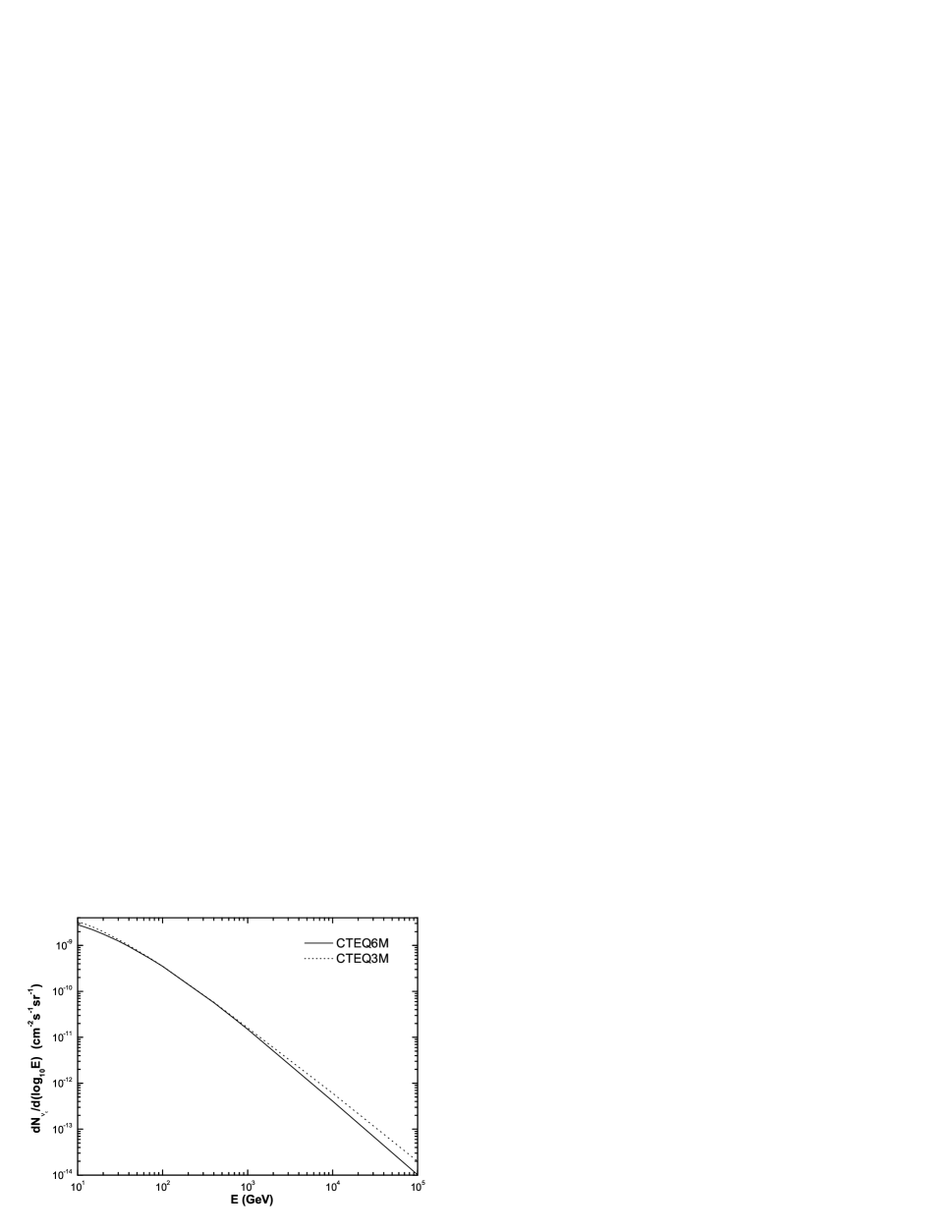
Figure 3: The comparison of intrinsic atmospheric $\nu_{\tau}$ fluxes calculated by perturbative QCD with CTEQ3 and CTEQ6 parton distribution functions respectively.

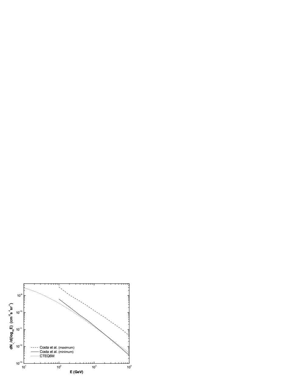
Figure 4: The model dependencies of intrinsic atmospheric $\nu_{\tau}$ flux. The minimal flux from Ref. Costa:2001fb is given by perturbative QCD. The maximal flux from the same reference is given by RQPM model for $E\leq 300$ GeV, and by QGSM model for $E>300$ GeV.

The uncertainty of intrinsic atmospheric $\nu_{\tau}$ flux due to different approaches for $Z_{pp}$ is negligible. The main uncertainty of this flux is due to the model dependence of the $Z$-moment $Z_{pD_{s}}$. Within the perturbative QCD approach, the dependence of this flux on the parton distribution functions is shown in Fig. 3. It is easily seen that the intrinsic atmospheric $\nu_{\tau}$ flux is not sensitive to parton distribution functions for $E<10^{3}$ GeV. However, at $E=10^{4}$ GeV, both fluxes differ by almost $50\%$. Incorporating the non-perturbative approaches for charm hadron productions Kaidalov:1985jg ; Bugaev:1998bi , the uncertainties of intrinsic atmospheric $\nu_{\tau}$ flux is depicted in Fig. 4. It is seen that the minimal $\nu_{\tau}$ flux in Ref. Costa:2001fb is consistent with our $\nu_{\tau}$ flux calculated by perturbative QCD with CTEQ6 parton distribution functions. On the other hand, the maximal flux shown in Fig. 4 is almost one order of magnitude larger than the minimal one. This maximal flux is given by the RQPM model below 300 GeV while it is given by the QGSM model beyond this energy Costa:2001va . We remark that the original minimal and maximal $\nu_{\tau}$ fluxes in Ref. Costa:2001fb correspond to different sets of primary cosmic ray flux, which is considered as one of the uncertainties for the $\nu_{\tau}$ flux. However, we have re-scaled these fluxes to a common cosmic ray flux, Eq. (2), used in this paper. We also note that the uncertainty of intrinsic atmospheric $\nu_{\tau}$ flux provided by Ref. Costa:2001fb starts at $E=100$ GeV, while our calculation of this flux starts at $E=10$ GeV.

It is interesting to see how much the uncertainty of the intrinsic $\nu_{\tau}$ flux could affect the determination of the $\nu_{\tau}$ flux taking into account the oscillation effect. In the next section, we shall study this issue with respect to the upward atmospheric $\nu_{\tau}$ flux where the oscillation effect is the largest.

III The Atmospheric Tau Neutrino Flux with Oscillations

III.1 The Downward and Horizontal Atmospheric Tau Neutrino Fluxes

The atmospheric tau neutrino flux can be calculated using

$$\frac{\mbox{d}\bar{N}_{\nu_{\tau}}(E,\xi)}{\mbox{d}E} = \int_{0}^{X_{\rm max}(\xi)}{\mbox{d}}X\left[\frac{\mbox{d}^{2}N_{\nu_{\mu}}(E,\xi,X)}{\mbox{d}E\mbox{d}X}\cdot P_{\nu_{\mu}\to\nu_{\tau}}\left(E,L(X,\xi)\right)\right.$$ (17)

$$\left.+\frac{\mbox{d}^{2}N_{\nu_{\tau}}(E,\xi,X)}{\mbox{d}E\mbox{d}X}\cdot\left(1-P_{\nu_{\mu}\to\nu_{\tau}}\left(E,L(X,\xi)\right)\right)\right],$$

where $P_{\nu_{\mu}\to\nu_{\tau}}\left(E,L(X,\xi)\right)\equiv\sin^{2}2\theta_{23}\sin^{2}(1.27\Delta m_{31}^{2}L/E)$ is the $\nu_{\mu}\to\nu_{\tau}$ oscillation probability, assuming a vanishing $\theta_{13}$. We have used the notation $\mbox{d}\bar{N}_{\nu_{\tau}}(E,\xi)/\mbox{d}E$ to denote the atmospheric $\nu_{\tau}$ flux taking into account the oscillation effect. The unit of $\Delta m_{31}^{2}$ is eV² while $L$ and $E$ are in units of km and GeV respectively. A recent SK analysis of the atmospheric neutrino data implies Ashie:2004mr

$$\Delta m_{31}^{2}=(1.9-3.0)\cdot 10^{-3}\,\,\,{\rm eV}^{2},\,\,\,\sin^{2}2\theta_{23}>0.9.$$ (18)

This is a $90\%\,{\rm C.L.}$ range with the best fit values given by $\Delta m_{31}^{2}=2.4\cdot 10^{-3}\,\,\,{\rm eV}^{2}$ and $\sin^{2}2\theta_{23}=1$ respectively.

III.1.1 Meson decay contributions

Using the best fit values of neutrino oscillation parameters, we obtain atmospheric tau neutrino fluxes for $\cos\xi=0.2,\ 0.4,\ \cdots,\ 1$ as depicted in Fig. 5. This set of result is obtained by using an energy-independent $Z$ moment, $Z_{pp}\equiv 1-\lambda_{p}/\Lambda_{p}=0.263$ mentioned earlier. For the $\nu_{\mu}$ flux on the R.H.S. of Eq. (17), we only include the two-body pion and kaon decay contributions. The muon-decay contribution to this flux will be presented later. The intrinsic $\nu_{\tau}$ flux in the same equation is taken to be that calculated by perturbative QCD with CTEQ6 parton distribution functions Pumplin:2002vw . It is instructive to separately present the oscillated and intrinsic atmospheric $\nu_{\tau}$ fluxes corresponding to the two terms on the R.H.S. of Eq. (17). This is done for $\xi=0^{\circ}$ in Fig. 6. We see that the oscillated and intrinsic atmospheric $\nu_{\tau}$ fluxes cross at $E\simeq 20$ GeV, indicating that the $\nu_{\mu}\to\nu_{\tau}$ oscillation effect becomes important for $E<20$ GeV for such a zenith angle.

We note that the atmospheric $\nu_{\tau}$ flux increases as $\xi$ increases from $0^{\circ}$ to $90^{\circ}$. There are two crucial factors dictating the angular dependence of such a flux. First, the atmosphere depth traversed by the cosmic ray particles increases as the zenith angle $\xi$ increases. Second, the atmospheric muon neutrinos are on-average produced more far away from the ground detector for a larger zenith angle, implying a larger $\nu_{\mu}\to\nu_{\tau}$ oscillation probability. In fact, the neutrino path-length dependencies on the zenith angle $\xi$ and the neutrino energy $E$ have been studied carefully by the Monte-Carlo simulation Gaisser:1997eu . Our semi-analytic approach reproduces these dependencies very well. It is found that, for $E=10$ GeV and $\cos\xi=1$ ($\xi=0^{\circ}$), the average neutrino path-length from the $\nu_{\mu}$ production point to the ground detector is $14$ km. The average neutrino path-length increases to $45$ km and $650$ km for $\xi=66^{\circ}$ ($\cos\xi=0.4$) and $\xi=90^{\circ}$ respectively. The huge path-length of horizontal neutrinos makes the $\nu_{\tau}$ flux in this direction two orders of magnitude larger than the downward $\nu_{\tau}$ flux. It is also interesting to note that the horizontal $\nu_{\tau}$ flux for $E$ approaching $1$ GeV begins to show oscillatory behavior. This is because, for $E=1$ GeV and $\Delta m_{31}^{2}=2.4\cdot 10^{-3}$ eV², $L_{\rm osc}\equiv 4E/\Delta m_{31}^{2}\approx 330$ km which is already shorter than the average neutrino path-length at this zenith angle.

We stress that our calculation procedures for $\cos\xi>0.5$ and $\cos\xi<0.5$ are different. In the former case, the curvature of the Earth can be neglected and the pion or kaon survival probability in the atmosphere is approximated by Eq. (5). This is the approach we adopted in Ref. Athar:2004um . For $\cos\xi<0.5$, i.e., $\xi>60^{\circ}$, we use Eq. (4) for the meson survival probability. In this case the calculation is much more involved as the meson survival probability in Eq. (4) contains an additional integration. It has been pointed out in Ref. Gaisser:1997eu that one may apply Eq. (5) for calculating the path-length distribution of neutrinos for $\xi>60^{\circ}$ so long as one replaces $\cos\xi$ by $\cos_{\rm eff}\xi$, where the latter is a fitted function of the former. Precisely speaking, by fitting the analytic calculation based upon Eq. (5) Lipari:1993hd to the Monte-Carlo calculation, the relations between $\cos\xi$ and $\cos_{\rm eff}\xi$ can be found, which are tabulated in Gaisser:1997eu . Extrapolating such a relation, we find that $\cos_{\rm eff}\xi=0.05$ for $\cos\xi=0$. Using this $\cos_{\rm eff}\xi$ with Eq. (5), we also calculate the atmospheric $\nu_{\tau}$ flux. The result is compared with that obtained by the full calculation (applying Eq. (4)) as shown in Fig. 7. Both results agree very well. Such an agreement makes our calculation compelling and also validates the above extrapolation on $\cos_{\rm eff}\xi$.

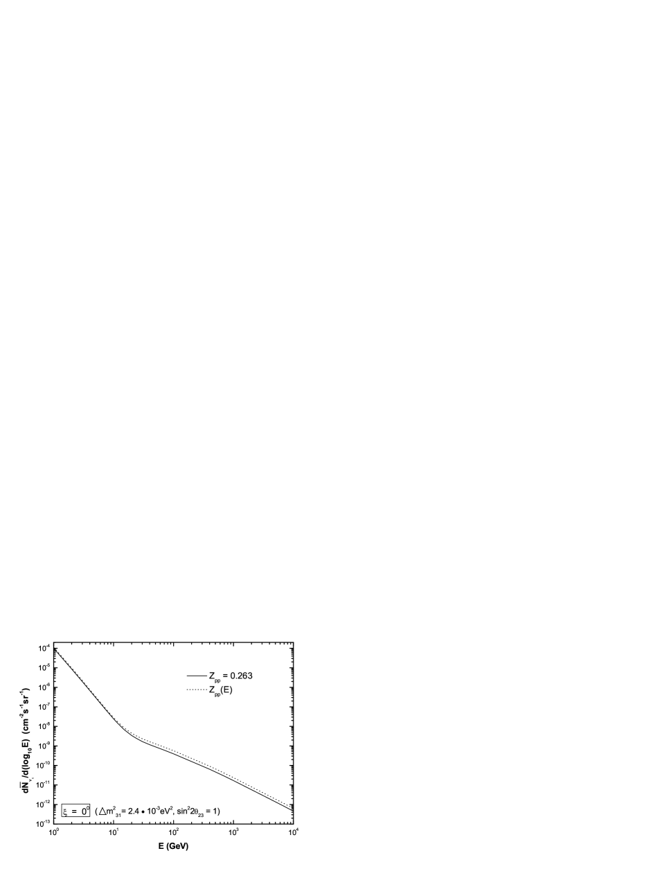
Figure 8: The comparison of atmospheric $\nu_{\tau}$ fluxes calculated from a constant $Z_{pp}$ COSMIC ; Lipari:1993hd and an energy-dependent $Z_{pp}$ Gondolo:1995fq for $\xi=0^{\circ}$.

We have so far computed the atmospheric neutrino flux with an energy independent $Z$ moment, $Z_{pp}\equiv 1-\lambda_{p}/\Lambda_{p}=0.263$. It is important to check the sensitivity of atmospheric $\nu_{\tau}$ flux on the values of $Z_{pp}$. We recall that different results for $Z_{pp}$ are shown in Fig. 1. At energies between $10^{2}$ GeV and $10^{3}$ GeV, the values of $Z_{pp}$ generated by PYTHIA pythia slightly depend on the energy and roughly twice larger than the value we have so far used for calculations. We check the effect of $Z_{pp}$ by calculating the atmospheric $\nu_{\tau}$ flux with the PYTHIA-generated $Z_{pp}$. The comparison of this result with the earlier one obtained by setting $Z_{pp}=0.263$ is shown in Fig. 8 for $\xi=0^{\circ}$ and Fig. 9 for $\xi=90^{\circ}$. For $\xi=0^{\circ}$, two set of results do not exhibit noticeable difference until $E\geq 10$ GeV. At $E=100$ GeV, they differ by $45\%$. For $\xi=90^{\circ}$, two results differ by $46\%$ at $E=1$ GeV while they differ by $29\%$ at $E=100$ GeV. Obviously, the behavior of $Z_{pp}$ is one of the major uncertainties for determining the atmospheric $\nu_{\tau}$ flux.

III.1.2 Muon-Decay contributions

We have stated that the muon-decay contributions to $\nu_{\mu}$ is non-negligible for neutrino energies less than $10$ GeV. Such $\nu_{\mu}$’s can oscillate into $\nu_{\tau}$’s during their propagations in the atmosphere. The calculation of such a flux according to Eqs. (6) and (10) is rather involved. However, a simple approximation as presented below gives a rather accurate result for this flux.

The calculation of $\nu_{\mu}$ spectrum due to muon decays requires the knowledge of muon polarizations. The muon polarization however depends on the ratio of muon momentum to the momentum of parent pion or kaon as indicated by Eq. (9). It is straightforward to calculate the average muon polarization at any slant depth $X$ provided the energy spectrum of the parent pion or kaon is known at that point. For the downward case ($\xi=0^{\circ}$), it is known from the previous section that the muons are most likely produced at around $14$ km from the ground detector. At that point, the pion and kaon fluxes can be approximately parameterized as $\phi_{\pi}(E_{\pi})=10^{-3.15}\cdot E_{\pi}^{-2.02}$ and $\phi_{K}(E_{K})=10^{-5.11}\cdot E_{K}^{-1.74}$ in units of cm^-2s^-1sr^-1GeV^-1 for meson energies between $1$ and few tens of GeV. We do not distinguish $\pi^{-}(K^{-})$ from $\pi^{+}(K^{+})$ in the above fittings. Although the spectra are charge dependent, the resulting absolute values of $\mu^{+}$ polarization and $\mu^{-}$ polarization differ by only $10\%$ for $E_{\mu}$ up to few tens of GeV Lipari:1993hd . From Eq. (9), and the above pion and kaon spectra, we obtain $\langle P_{\mu^{-}}^{\pi}\rangle=0.35$, $\langle P_{\mu^{-}}^{K}\rangle=0.95$. Therefore $\mu^{-}$ coming from the $\pi^{-}$ decays are $67\%$ right-handed polarized and $33\%$ left-handed polarized. On the other hand, $\mu^{-}$ coming from $K^{-}$ decays are $98\%$ right-handed polarized and only $2\%$ left-handed polarized. The muons produced by meson decays lose energies before they decay into neutrinos. The decay distribution for $\mu^{-}\to\nu_{\mu}$ is given by Eq. (11). The average momentum fraction $\langle y\rangle$ of muon neutrinos are $0.3$ and $0.4$ from decays of right-handed $\mu^{-}$ and left-handed $\mu^{-}$ respectively. Following a similar procedure, one can determine the polarization and decay distributions of $\mu^{+}$. Finally, to calculate the spectrum of muon neutrinos arising from muon decays, we use the approximation of replacing $F_{\mu^{\pm}_{s}\to\nu_{\mu}}(E/E_{\mu})$ with $\delta(E/E_{\mu}-\langle y\rangle)$ in Eq. (10).

To check the validity of the above approximation, we compare our result on the fraction of muon decay contribution to the overall $\nu_{\mu}$ flux with that given by Ref. Lipari:1993hd for $\cos\xi=0.4$, i.e., $\xi=66^{\circ}$. At this zenith angle, most of the muons are produced roughly $45$ km from the detector. The pion and kaon fluxes at this point are fitted to be $\phi_{\pi}(E_{\pi})=10^{-3.65}\cdot E_{\pi}^{-1.88}$ and $\phi_{K}(E_{K})=10^{-5.57}\cdot E_{K}^{-1.69}$ in units of cm^-2s^-1sr^-1GeV^-1. This gives rise to $\langle P_{\mu^{-}}^{\pi}\rangle=0.34$, $\langle P_{\mu^{-}}^{K}\rangle=0.94$. Following the procedure in the downward case, we obtain the muon neutrino flux from the muon decays. At $E=1$ GeV, the fraction of muon-decay contributions to the overall $\nu_{\mu}$ flux is $44\%$ while the fraction decreases to $17\%$ at $E=10$ GeV. In Ref. Lipari:1993hd , the corresponding fractions are $47\%$ and $18\%$ respectively. Both set of fractions agree rather well.

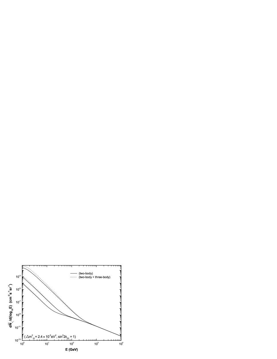
Figure 10: The comparisons of atmospheric $\nu_{\tau}$ fluxes resulting from the oscillations of $\nu_{\mu}$’s generated by two-body and three-body decays with those resulting from the oscillations of $\nu_{\mu}$’s generated only by two-body decays. The comparisons are made for three zenith angles, $\cos\xi=0,\ 0.4$, and $1$ (from top to bottom).

Since our approximation works well for calculating the muon-decay contributions to the atmospheric $\nu_{\mu}$ flux, we proceed to calculate the resulting atmospheric $\nu_{\tau}$ flux with Eq. (17). Specifically we only need to include the first term on the R.H.S. of Eq. (17) because the second term has already been included in the two-body decay contribution. In Fig. 10, those atmospheric $\nu_{\tau}$ fluxes resulting from oscillations of $\nu_{\mu}$’s generated by both two- and three-body decays (muon decays) are compared with those resulting from the oscillations of $\nu_{\mu}$’s generated only by two-body decays. As expected, the three-body decay contribution is non-negligible for $E\leq 10$ GeV. Quantitatively, for $\xi=0^{\circ}$ and $E=1$ GeV, $24\%$ of the total atmospheric $\nu_{\tau}$ flux is from the oscillations of $\nu_{\mu}$’s originated from the muon decays. At $E=10$ GeV, only $2.9\%$ of the total atmospheric $\nu_{\tau}$ flux comes from the same source. For $\xi=66^{\circ}$, the three-body decay contribution gives rise to $36\%$ and $8.9\%$ of the total atmospheric $\nu_{\tau}$ flux at $E=1$ GeV and $E=10$ GeV respectively. Finally, for $\xi=90^{\circ}$, the three-body decay contribution to the total atmospheric $\nu_{\tau}$ flux is most significant. It contributes to $53\%$, $46\%$, and $39\%$ of the total atmospheric $\nu_{\tau}$ flux at $E=1$ GeV, $10$ GeV and $20$ GeV respectively. To calculate the three-body decay contribution to $\nu_{\mu}$ flux at $\xi=90^{\circ}$, we have used Eq. (5) for the meson survival probability with $\cos_{\rm eff}\xi=0.05$ and a overall factor $C\approx 1.40$ to fix the normalization of the flux Gaisser:1997eu .

III.2 The Upward Atmospheric Tau Neutrino Flux

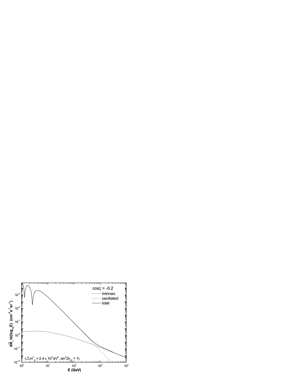
Figure 11: The atmospheric $\nu_{\tau}$ flux (solid line) as a sum of its oscillated (dotted line) and intrinsic (dashed line) components for $\cos\xi=-0.2$ with $\sin^{2}2\theta_{23}=1$, $\Delta m_{31}^{2}=2.4\cdot 10^{-3}\,\,\,{\rm eV}^{2}$, and $Z_{pp}=0.263$.

The upward atmospheric $\nu_{\tau}$ fluxes are enhanced compared to those of other directions since the average neutrino path lengths in such case are larger. Therefore the observations of astrophysical tau neutrinos in upward directions are subject to more serious background problems. However, observing the atmospheric tau neutrinos is interesting in its own right. The atmospheric tau neutrino flux for $\cos\xi=-0.2$ is shown in Fig. 11. The effect of $\nu_{\mu}\to\nu_{\tau}$ oscillation is evident for below TeV energies. This is seen from the crossing point of intrinsic and oscillated atmospheric $\nu_{\tau}$ fluxes at $E\simeq 700$ GeV. The atmospheric $\nu_{\tau}$ flux shows oscillatory behavior for $E\leq 10$ GeV. For $\cos\xi<-0.2$, such an oscillatory behavior is even more significant. In such a case, it is more practical to study the averaged flux. We average the atmospheric $\nu_{\tau}$ flux for the zenith angle range $-1\leq\cos\xi\leq-0.4$, as shown in Fig. 12. Due to uncertainties of the intrinsic atmospheric $\nu_{\tau}$ flux as discussed in Ref. Costa:2001fb , the atmospheric $\nu_{\tau}$ flux taking into account the oscillation effect also contains uncertainties beginning at a few hundred GeV’s. In the same figure, we also plot the corresponding atmospheric $\nu_{\mu}$ flux. The $\nu_{\mu}$ and $\nu_{\tau}$ fluxes are comparable for $E<40$ GeV. In such a case, the footprint of $\nu_{\tau}$ might be identified by studying the energy spectra of shower events induced by neutrino interactions Stanev:1999ki . At $E=10^{4}$ GeV, the $\nu_{\mu}$ flux is approximately $30$ times larger than the maximal $\nu_{\tau}$ flux. We note that the maximal and minimal $\nu_{\tau}$ fluxes begin to differ at $E=500$ GeV. At $E=1$ TeV, the maximal flux is $3$ times larger than the minimal one. The ratio of maximal flux to the minimal one increases to $14$ at $E=10$ TeV. We remark that the upward atmospheric $\nu_{\tau}$ flux is also calculated in Ref. Stanev:1999ki with $\sin^{2}2\theta_{23}=1$ and $\Delta m_{31}^{2}=10^{-2},\ 10^{-2.5},\ 10^{-3}$ eV² respectively. Here we have done the calculation with the best fit value of $\sin^{2}2\theta_{23}$ and $\Delta m_{31}^{2}$ taken from Ashie:2004mr . Furthermore we include the contribution of intrinsic atmospheric $\nu_{\tau}$ flux and its associated uncertainties.

IV Discussion and Conclusion

The understanding of atmospheric $\nu_{\tau}$ flux is important for exploring the tau neutrino astronomy Athar:2004pb ; Athar:2004um . As mentioned earlier, an estimation of the atmospheric $\nu_{\tau}$ flux has been given in Ref. Athar:2004pb while a detailed calculation of this flux for zenith angles $0\leq\xi\leq 60^{\circ}$ is given in Ref. Athar:2004um . In these works, comparisons of the galactic-plane $\nu_{\tau}$ flux with the atmospheric $\nu_{\tau}$ flux are also made for illustrating the possibility of the tau neutrino astronomy. Now that we have obtained a complete result of the atmospheric $\nu_{\tau}$ flux for the entire zenith angle range, we compare this flux with two astrophysical fluxes: the galactic-plane tau neutrino flux just mentioned and the cosmological $\nu_{\tau}$ flux due to neutralino dark matter annihilations Elsaesser:2004ck . The comparison is depicted in Fig. 13 where the flux of galactic-plane tau neutrinos is taken from the calculation of Ref. Athar:2004um . One can see that the galactic-plane $\nu_{\tau}$ flux dominates over the downward ($\xi=0^{\circ}$) atmospheric $\nu_{\tau}$ flux for $E$ greater than a few GeV. Hence, in this direction, it is possible to observe the flux of galactic-plane tau neutrinos in the GeV energy range. For near horizontal directions, the atmospheric $\nu_{\tau}$ flux grows rapidly with zenith angles. Therefore, for $\xi=90^{\circ}$, the energy threshold for galactic-plane tau neutrino flux to dominate over its atmospheric counterpart is pushed up to $E\simeq 100$ GeV. We further see that the galactic-plane $\nu_{\tau}$ flux does not dominate the upward atmospheric $\nu_{\tau}$ background ($-1\leq\cos\xi\leq-0.4$) until $E=500$ GeV. However, it is noteworthy that, in the muon neutrino case, galactic-plane neutrino flux is overwhelmed by the atmospheric background until $E_{\nu}>10^{6}$ GeV Athar:2003nc . Such a difference between $\nu_{\mu}$ and $\nu_{\tau}$ shows the promise of the tau neutrino astronomy in the GeV energy range as pointed out in Athar:2004pb ; Athar:2004um . From Fig. 13, it is also clear that the atmospheric $\nu_{\tau}$ flux is a non-negligible background to the cosmological tau neutrino flux due to neutralino dark matter annihilations Elsaesser:2004ck . In fact, two fluxes are comparable in the downward direction while the atmospheric $\nu_{\tau}$ flux dominates in horizontal and upward directions.

In summary, we have presented a semi-analytical calculation on the atmospheric $\nu_{\tau}$ flux in the GeV to TeV energy range for downward, upward, and horizontal directions. The atmospheric $\nu_{\tau}$ flux at $\xi=90^{\circ}$ is two orders of magnitude larger than the corresponding flux at $\xi=0^{\circ}$ for $1\leq E/{\rm GeV}\leq 10$. On the other hand, the fluxes with zenith angles between $0$ and $90$ degrees merge for $E\geq 700$ GeV, provided that the intrinsic atmospheric $\nu_{\tau}$ flux is calculated with perturbative QCD. Should one adopt a non-perturbative model for the intrinsic $\nu_{\tau}$ flux, the resulting $\nu_{\tau}$ fluxes on Earth at different zenith angles would merge at an energy lower than $700$ GeV. We have observed that the upward atmospheric $\nu_{\tau}$ fluxes show oscillatory behaviors. For the averaged flux with $-1\leq\cos\xi\leq-0.4$, the atmospheric $\nu_{\tau}$ flux is found to be comparable to the atmospheric $\nu_{\mu}$ flux for $E<40$ GeV. The comparison of this flux with the horizontal atmospheric $\nu_{\tau}$ flux is also interesting. Two fluxes are in fact comparable for $E<10$ GeV. This shows that the $\nu_{\mu}\to\nu_{\tau}$ oscillation is already quite significant in the horizontal direction for such an energy range. Nevertheless, the upward atmospheric $\nu_{\tau}$ flux takes over from $E\geq 10$ GeV until $E\simeq 3$ TeV where two fluxes merge again. Concerning the uncertainties in our calculations, we have studied the dependencies of atmospheric $\nu_{\tau}$ flux on the $Z$ moment $Z_{pp}$ for representative zenith angles $\xi=0^{\circ}$ and $\xi=90^{\circ}$. We have also discussed in detail the uncertainty of intrinsic atmospheric $\nu_{\tau}$ flux due to different models for charm hadron productions. The consequence of such a uncertainty on the determination of oscillated $\nu_{\tau}$ flux is studied as well. Concerning the technique for calculating the atmospheric $\nu_{\tau}$ flux from large zenith angles, we have verified the validity of using $\cos_{\rm eff}\xi$ in Eq. (5) to calculate the atmospheric $\nu_{\tau}$ flux for $\xi>60^{\circ}$. In particular, we have extrapolated the results in Ref. Gaisser:1997eu to $\xi=90^{\circ}$ and demonstrate that the choice $\cos_{\rm eff}(\xi=90^{\circ})=0.05$ reproduces well the atmospheric $\nu_{\tau}$ flux obtained by a full calculation using Eq. (4).

Figure 1: The comparison of $Z_{pp}$ obtained by assuming the Feynman scaling COSMIC and that obtained by PYTHIA Gondolo:1995fq . Our extrapolation of the latter result is also shown.

Figure 5: The atmospheric $\nu_{\tau}$ flux for $\cos\xi=0,\ 0.2,\ 0.4,\ 0.6,\ 0.8$ and $1$ (from top to bottom) with $\sin^{2}2\theta_{23}=1$, $\Delta m_{31}^{2}=2.4\cdot 10^{-3}\,\,\,{\rm eV}^{2}$, and $Z_{pp}=0.263$.

Figure 6: The downward atmospheric $\nu_{\tau}$ flux (solid line) as the sum of its oscillated (dotted line) and intrinsic (dashed line) components.

Figure 9: The comparison of atmospheric $\nu_{\tau}$ fluxes calculated from a constant $Z_{pp}$ COSMIC ; Lipari:1993hd and an energy-dependent $Z_{pp}$ Gondolo:1995fq for $\xi=90^{\circ}$.

Figure 12: The atmospheric $\nu_{\tau}$ flux averaged for $-1\leq\cos\xi\leq-0.4$. The uncertainty of this flux due to the uncertainty of intrinsic atmospheric $\nu_{\tau}$ flux is shown. The corresponding $\nu_{\mu}$ flux is also plotted, which is equal to the $\nu_{\tau}$ flux for $1\leq E/{\rm GeV}\leq 10$.

Figure 13: The comparison of atmospheric $\nu_{\tau}$ fluxes with the galactic-plane tau neutrino flux Athar:2004um and the tau neutrino flux due to the neutralino dark matter annihilations Elsaesser:2004ck . We have included downward ($\cos\xi=1$), horizontal ($\cos\xi=0$) and upward ($-1\leq\cos\xi\leq-0.4$) atmospheric $\nu_{\tau}$ fluxes for the comparison. At $E=1$ GeV, the horizontal flux is the largest whereas the downward flux is the smallest.

References

- (1) For a recent result, see Y. Ashie et al. [Super-Kamiokande Collaboration], Phys. Rev. Lett. 93, 101801 (2004) [arXiv:hep-ex/0404034].
- (2) H. Athar, Mod. Phys. Lett. A 19, 1171 (2004).
- (3) H. Athar and C. S. Kim, Phys. Lett. B 598, 1 (2004) [arXiv:hep-ph/0407182].
- (4) For a recent review, see G. Bertone, D. Hooper and J. Silk, Phys. Rept. 405, 279 (2005) [arXiv:hep-ph/0404175].
- (5) T. Stanev, Phys. Rev. Lett. 83, 5427 (1999) [arXiv:astro-ph/9907018].
- (6) A. Zalewska [ICARUS Collaboration], Acta Phys. Polon. B 35, 1949 (2004).
- (7) J. Campagne, Eur. Phys. J. C 33, S837 (2004).
- (8) T. K. Gaisser and M. Honda, Ann. Rev. Nucl. Part. Sci. 52, 153 (2002) [arXiv:hep-ph/0203272].
- (9) For an estimation of the same flux in the three-flavor neutrino oscillation framework, see H. Athar, arXiv:hep-ph/0411303.
- (10) H. Athar, F. F. Lee and G. L. Lin, Phys. Rev. D 71, 103008 (2005) [arXiv:hep-ph/0407183].
- (11) T. K. Gaisser, Astropart. Phys. 16, 285 (2002) [arXiv:astro-ph/0104327].
- (12) Cosmic Rays and Particle Physics, T. K. Gaisser, Cambridge University Press (1992).
- (13) P. Lipari, Astropart. Phys. 1, 195 (1993).
- (14) T. , Comput. Phys. Commun. 82, 74 (1994).
- (15) M. Thunman, G. Ingelman and P. Gondolo, Astropart. Phys. 5, 309 (1996) [arXiv:hep-ph/9505417].
- (16) V. Agrawal, T. K. Gaisser, P. Lipari and T. Stanev, Phys. Rev. D 53, 1314 (1996) [arXiv:hep-ph/9509423].
- (17) B. Rossi, High Energy Particles (Prentice Hall, Englewood Cliffs, NJ, USA, 1952).
- (18) S. M. Barr, T. K. Gaisser, P. Lipari and S. Tilav, Phys. Lett. B 214, 147 (1988).
- (19) G. Barr, T. K. Gaisser and T. Stanev, Phys. Rev. D 39, 3532 (1989).
- (20) L. Pasquali and M. H. Reno, Phys. Rev. D 59, 093003 (1999) [arXiv:hep-ph/9811268].
- (21) P. Nason, S. Dawson and R. K. Ellis, Nucl. Phys. B 327, 49 (1989) [Erratum-ibid. B 335, 260 (1990)].
- (22) M. L. Mangano, P. Nason and G. Ridolfi, Nucl. Phys. B 373, 295 (1992).
- (23) J. Pumplin, D. R. Stump, J. Huston, H. L. Lai, P. Nadolsky and W. K. Tung, JHEP 0207, 012 (2002) [arXiv:hep-ph/0201195].
- (24) L. Pasquali, M. H. Reno and I. Sarcevic, Phys. Rev. D 59, 034020 (1999) [arXiv:hep-ph/9806428].
- (25) A. B. Kaidalov and O. I. Piskunova, Z. Phys. C 30, 145 (1986); L. V. Volkova, W. Fulgione, P. Galeotti and O. Saavedra, Nuovo Cim. C 10, 465 (1987).
- (26) E. V. Bugaev, A. Misaki, V. A. Naumov, T. S. Sinegovskaya, S. I. Sinegovsky and N. Takahashi, Phys. Rev. D 58, 054001 (1998) [arXiv:hep-ph/9803488].
- (27) C. G. S. Costa, Astropart. Phys. 16, 193 (2001) [arXiv:hep-ph/0010306].
- (28) C. G. S. Costa, F. Halzen and C. Salles, Phys. Rev. D 66, 113002 (2002) [arXiv:hep-ph/0104039].
- (29) B. A. Li, Phys. Rev. D 52, 5165 (1995) [arXiv:hep-ph/9504304].
- (30) C. G. S. Costa and C. Salles, arXiv:hep-ph/0105271.
- (31) T. K. Gaisser and T. Stanev, Phys. Rev. D 57, 1977 (1998) [arXiv:astro-ph/9708146].
- (32) D. Elsaesser and K. Mannheim, Astropart. Phys. 22, 65 (2004) [arXiv:astro-ph/0405347].
- (33) H. Athar, K. Cheung, G. L. Lin and J. J. Tseng, Eur. Phys. J. C 33, S959 (2004) [arXiv:astro-ph/0311586].