Interactions of cosmic neutrinos with nucleons in the RS model

Abstract

We consider the scattering of the brane fields due to $t$-channel massive graviton exchanges in the Randall-Sundrum model. The eikonal amplitude is analytically calculated and both differential and total neutrino-nucleon cross sections are estimated. The event rate of quasi-horizontal air showers induced by cosmic neutrinos, which can be detected at the Pierre Auger Observatory, is presented for two different fluxes of cosmogenic neutrinos.

1 Introduction

The detection of air showers induced by ultra-high energy neutrinos may help to solve many important problems, such as propagation of cosmic neutrinos to the Earth and their interactions with the nucleons at energies around tens (hundreds) of TeV. In this energy region, neutrino-nucleon interactions may be strong due to a new physics. There is a large class of models in a space-time with extra spacial dimensions which result in a new TeV phenomenology. In the present paper we will consider an approach with non-factorizable metric proposed in Refs. [1, 2], and study a scattering of the SM fields in this scenario.

The RS model [1, 2] is a model of gravity in a slice of a 5-dimensional Anti-de-Sitter space (AdS₅) with a single extra dimension compactified to the orbifold $S^{1}/Z_{2}$. The metric is of the form:

$$ds^{2}=e^{-2\kappa|y|}\,\eta_{\mu\nu}\,dx^{\mu}\,dx^{\nu}+dy^{2}.$$ (1)

Here $y=r_{c}\theta$ ($0\leqslant\theta\leqslant\pi$), $r_{c}$ is a ”radius” of extra dimension, and parameter $\kappa$ defines the scalar (negative) curvature of the space.

From a 4-dimensional action one can derive the relation:

$$\bar{M}_{Pl}^{2}=\frac{M^{3}}{\kappa}\left(1-e^{-2\pi\kappa r}\right)\simeq\frac{M^{3}}{\kappa},$$ (2)

which means that $\kappa\sim\bar{M}_{Pl}\sim M$, with $M$ being a 5-dimensional Planck scale.

We will consider so-called RS1 model [1] which has two 3-dimensional branes with equal but opposite in sign tensions which are located at the point $y=\pi r_{c}$ (called the TeV brane) and at the point $y=0$ (referred to as the Planck brane). All SM fields are constrained to the TeV brane, while the gravity propagates in the bulk (all spacial dimensions).

From the point of view of an observer located on the TeV brane, there exists an infinite number of graviton Kaluza-Klein (KK) excitations with masses:

$$m_{n}=x_{n}\kappa\,e^{-\pi\kappa r_{c}},\qquad n=1,2\ldots,$$ (3)

where $x_{n}$ are zeros of the Bessel function $J_{1}(x)$:

$$J_{1}(x_{n})=0,\qquad n=1,2\ldots$$ (4)

By using a linear expansion of the metric, one can derive the interaction Lagrangian:

$$\mathcal{L}=-\frac{1}{\bar{M}_{Pl}}\,T_{\mu\nu}\,h^{(0)}_{\mu\nu}-\frac{1}{\Lambda_{\pi}}\,T_{\mu\nu}\,\sum_{n=1}^{\infty}h^{(n)}_{\mu\nu},$$ (5)

where

$$\Lambda_{\pi}=\bar{M}_{Pl}\,e^{-\pi\kappa r_{c}}$$ (6)

is a physical scale on the TeV brane. It can be chosen as small as 1 TeV for a thick slice of the AdS₅, $r_{c}\simeq 12/\kappa\simeq 60\,l_{Pl}$. We see from (5) that couplings of all massive states are only suppressed by $\Lambda_{\pi}^{-1}$, while the zero mode couples with usual strength defined by the reduced Planck mass $\bar{M}_{Pl}=M_{Pl}/\sqrt{8\pi}$.

The main phenomenological parameters of the model are the scale $\Lambda_{\pi}$ and the ratio

$$\mu=\frac{\kappa}{\bar{M}_{Pl}}.$$ (7)

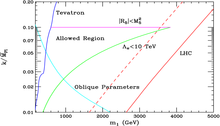
Figure 1: Experimental and theoretical constrains on the RS model in the two-parameter plane $\kappa/\bar{M}_{Pl}$ – $m_{1}$ [3]. The allowed region lies in the center as indicated.

The present experimental data together with theoretical bounds on the curvature of the AdS₅ restrict an allowed region for the variable $\mu$ (see, for instance, Fig. 1 taken from Ref. [3]):

$$0.01\lesssim\mu\lesssim 0.1.$$ (8)

The allowed value of $\mu$ is restricted by so-called naturalness and requiring a 5-dimensional curvature to be small enough to consider a linearized gravity on the brane. Thus, the lightest masses of the KK graviton modes, $m_{n}=x_{n}\mu\Lambda_{\pi}$, are of the order of 1 TeV.

Our paper has the following structure. In the next Section we consider interactions of the SM fields on the brane in the RS model induced by an exchange of massive gravitons. The eikonal amplitude is calculated and an elastic cross section for different sets of the RS parameters and/or invariant energy is estimated. In Sec. 3 we use these results to study the scattering of ultra-high energy cosmic neutrino off the atmospheric nucleons. The neutrino-nucleon cross section is calculated and an event rate of quasi-horizontal neutrino events expected at the Auger Observatory is presented. Our conclusions and discussions is a topic of Sect. 4.

2 Eikonal amplitude in the RS model

In what follows, we will employ the zero width approximation for the graviton KK resonances. The Born amplitude corresponding to $t$-channel exchange looks like (both the massless mode and KK gravitons contribute):

$$A_{B}(s,t)=\frac{8\pi G_{N}s^{2}}{-t}+\frac{s^{2}}{\Lambda_{\pi}^{2}}\sum_{n=1}^{\infty}\frac{1}{-t+m_{n}^{2}}.$$ (9)

The sum in (9) converges very rapidly in $n$, since $x_{n}=\pi\,(n+1/4)+\mathrm{O(n^{-1})}$ [7]. We consider the scattering of two particles living on the TeV brane. Thus, in Eq. (9) $t$ means a 4-dimensional momentum transfer which is well-defined and conserved.

Let us underline that in (9) we sum spin-two particles with different KK numbers $n$ (non-reggeized KK gravitons). In more general approach, one should sum Regge trajectories $\alpha_{n}(t)$ which are numerated by $n$ (KK-charged gravireggeons). For the ADD model, it was done in Refs. [13]. The results of Refs. [10, 13] can be reproduced in the limit $\alpha_{n}(t)\rightarrow 2$. As for the RS model, results on a gravireggeon contribution to the eikonal amplitude will be presented in a forthcoming paper [14].

Generally, the massive KK states may decay to a pair of SM particles. The partial widths are proportional to $m_{n}^{3}/\Lambda_{\pi}^{2}$, where $m_{n}$ is the mass of the resonance. In particular, the partial decay widths to massless gauge bosons, fermions, and a pair of Higgs are

$$\Gamma(h^{(n)}\rightarrow VV) = N_{V}\,a\,\frac{m_{n}^{3}}{40\pi\Lambda_{\pi}^{2}},$$

$$\Gamma(h^{(n)}\rightarrow f\bar{f}) = N_{f}\,\frac{m_{n}^{3}}{160\pi\Lambda_{\pi}^{2}},$$

$$\Gamma(h^{(n)}\rightarrow H\bar{H}) = \frac{m_{n}^{3}}{480\pi\Lambda_{\pi}^{2}}.$$ (10)

Here $N_{V}=1(8)$ for photons and electroweak bosons (gluons), $N_{f}=1(3)$ for a lepton (quark pair) mode, and $a=1/2$ for identical particles. Then for the total width of the massive KK graviton in the RS model, $\Gamma_{n}$, we get the estimate (see also [9]):

$$\Gamma_{n}\simeq m_{n}\,(0.31\,\mu\,x_{n})^{2}.$$ (11)

Since the sum which we are interested in converges very rapidly in $n$ (see a comment after Eq. (9)), we conclude from (11) and (8) that effectively $\Gamma_{n}/2\ll m_{n}$.

The sum (9) can be calculated analytically by the use of the formula [7]:

$$\sum_{n=1}^{\infty}\frac{1}{z_{n,\nu}^{2}-z^{2}}=\frac{J_{\nu+1}(z)}{2\,z\,J_{\nu}(z)},$$ (12)

where $z_{n,\,\nu}$ ($n=1,2\ldots$) are zeros of the function $z^{-\nu}J_{\nu}(z)$. As a result, we obtain:

$$A_{B}(s,t)=\frac{8\pi G_{N}s^{2}}{-t}+\frac{s^{2}}{2\mu\Lambda_{\pi}^{3}}\,\frac{1}{\sqrt{-t}}\,\frac{I_{2}(v)}{I_{1}(v)}$$ (13)

Here $I_{i}(z)$ ($i=1,2$) are modified Bessel functions and $v=\sqrt{-t}/\mu\Lambda_{\pi}$. Taking into account properties of $I_{i}(x)$, we conclude from (13) that a contribution of the massive graviton modes dominates at large $|t|$:

$$A_{B}(s,t)\Big{|}_{|t|\gg\mu\Lambda_{\pi}}\simeq\frac{s^{2}}{2\mu\Lambda_{\pi}^{3}}\,\frac{1}{\sqrt{|t|}}.$$ (14)

Note, we would get another asymptotics in $t$, namely, $A_{B}(s,t)\sim|t|^{-1}$, if we sum only finite number of the massive gravitons.

As it was shown in Ref. [10], it is ladder diagrams that makes a leading contribution of the KK gravitons to an amplitude and results in the eikonal representation for the amplitude ($q^{2}=-t$):

$$A^{eik}(s,t)=2is\!\int d^{2}b\,e^{iq\,b}\left[1-e^{i\chi(s,b)}\right],$$ (15)

with the eikonal given by

$$\chi(s,b)=\frac{1}{4\pi s}\int dq\,q\,J_{0}(q\,b)\,A_{B}(s,-q^{2}).$$ (16)

The proper accounting for the massless mode has been presented in Ref. [11]. The result is the following:

$$A^{eik}(s,t)=e^{i\phi_{4}}\,\Bigg{\{}\frac{8\pi G_{N}s}{-t}\,\frac{\Gamma(1-iG_{N}s)}{\Gamma(1+iG_{N}s)}$$

$$+\,4\pi is\,(-t)^{-iG_{N}s}\!\int\limits_{0}^{\infty}\,db\,b^{1-2iG_{N}s}\,J_{0}\left(b\sqrt{|t|}\right)\Big{[}1-e^{i\chi_{mass}(s,b)}\Big{]}\Bigg{\}}.$$ (17)

Here $\chi_{mass}(s,b)$ denotes a contribution the massive modes to the eikonal, $G_{N}$ is the Newton constant, and $\phi_{4}$ is a 4-dimensional (infinite) phase. The first term in the RHS of Eq. (2) is well-known 4-dimensional result derived by different methods in Refs. [12]. It is negligible at any conceivable energy and momentum transfer, and we can write (up to a phase factor):

$$A^{eik}(s,t)\simeq 4\pi is\!\int\limits_{0}^{\infty}\,db\,b\,J_{0}\left(b\sqrt{|t|}\right)\Big{[}1-e^{i\chi_{mass}(s,b)}\Big{]}.$$ (18)

It follows from (13) that the eikonal depends on two dimensionless variables, $s/\Lambda_{\pi}^{2}$, and

$$u=b\mu\Lambda_{\pi},$$ (19)

and it looks like

$$\tilde{\chi}_{mass}(s,u)\equiv\chi_{mass}(s,\frac{u}{\mu\Lambda_{\pi}})=\frac{1}{8\pi}\,\frac{s}{\Lambda_{\pi}^{2}}\!\int\limits_{0}^{\infty}\,dv\,J_{0}(uv)\,\frac{I_{2}(v)}{I_{1}(v)}.$$ (20)

The eikonal (20) is very well approximated by the following expression (see Appendix for details):

$$\tilde{\chi}_{mass}(s,u)\simeq\frac{\sqrt{3}}{16\pi}\,\frac{s}{u\Lambda_{\pi}^{2}}\,\exp(-2\sqrt{3}\,u).$$ (21)

At $\sqrt{s}\gg 5\,\Lambda_{\pi}$, the eikonal is exponentially small outside the region

$$b\lesssim b_{0}(s)=\frac{1}{\sqrt{3}\,\mu\Lambda_{\pi}}\,\ln\frac{\sqrt{s}}{\Lambda_{\pi}}.$$ (22)

At $b\rightarrow 0$, it is proportional to $b^{-1}$. Thus, we can roughly estimate the high-energy behavior of elastic cross section:

$$\sigma_{el}(s)\simeq\frac{\pi}{3\,(\mu\Lambda_{\pi})^{2}}\,\ln^{2}\frac{\sqrt{s}}{\Lambda_{\pi}}\thickapprox\frac{\pi}{m_{1}^{2}}\,\ln^{2}\frac{s}{\Lambda_{\pi}^{2}},$$ (23)

where $m_{1}$ is a mass of a lightest KK graviton.

Let us underline that the Froissart-Martin like formula (23) describes the contribution of the massive graviton modes. The presence of the massless graviton in the theory should result in infinite elastic and total cross sections [15]. However, its contribution can be safely neglected in our further calculations.

We can rewrite Eq. (18) in the form

$$A^{eik}(s,t)\simeq 4\pi i\,\frac{s}{(\mu\Lambda_{\pi})^{2}}\!\int\limits_{0}^{\infty}\,du\,u\,J_{0}\left(u\frac{\sqrt{-t}}{\mu\Lambda_{\pi}}\right)\Big{[}1-e^{i\tilde{\chi}_{mass}(s,u)}\Big{]}.$$ (24)

Correspondingly, the differential cross section in dimensionless variable

$$y=\frac{-t}{s}$$ (25)

is defined by

$$\frac{d\sigma_{el}}{dy}=\frac{1}{16\pi s}\,|A^{eik}(s,-ys)|^{2},$$ (26)

and we get the estimate

$$\frac{d\sigma_{el}}{dy}\Big{|}_{y=0}\simeq\frac{\pi\,s}{36\,(\mu\Lambda_{\pi})^{4}}\,\ln^{4}\frac{\sqrt{s}}{\Lambda_{\pi}}.$$ (27)

It follows from (26), (24) that $d\sigma_{el}/dy$ depends only on variable $y$ (25), parameter $\mu$, and the ratio $\sqrt{s}/\Lambda_{\pi}$, in addition to the dimensional factor $(\mu\Lambda_{\pi})^{-2}$ which defines a magnitude of the cross section. In particular, we have $d\sigma_{el}/dy|_{y=0}=s\,(\mu\Lambda_{\pi})^{-4}\,f(s/\Lambda_{\pi}^{2})$, and $\sigma_{el}=(\mu\Lambda_{\pi})^{-2}\,g(s/\Lambda_{\pi}^{2},\,\mu)$, were $f(x)$ and $g(x,y)$ are dimensionless functions defined via the eikonal.

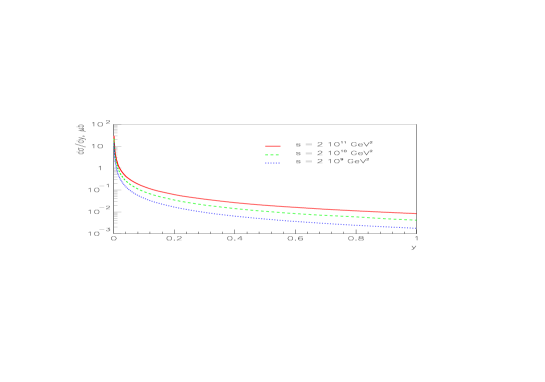
Figure 2: The differential cross section as a function of dimensionless variable $y$ for three fixed values of the invariant energy. The parameters of the RS model are chosen to be $\Lambda_{\pi}=$ 2 TeV, and $\mu=0.05$.

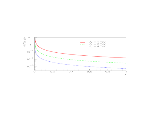
Figure 3: The differential cross section as a function of variable $y$ for three values of the mass scale $\Lambda_{\pi}$ at fixed energy $s=2\cdot 10^{11}$ GeV² (with the parameter $\mu=0.1$).

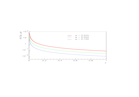
Figure 4: The differential cross section as a function of variable $y$ for three values of the RS parameter $\mu$ at fixed energy $s=2\cdot 10^{10}$ GeV² (with the scale $\Lambda_{\pi}=$ 1 TeV).

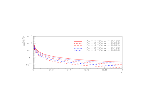
Figure 5: The reduced (dimensionless) differential cross section as a function of variable $y$ for different parameter sets ($\Lambda_{\pi}$, $\mu$) at invariant energy $s=2\cdot 10^{10}$ GeV². The product $\mu\Lambda_{\pi}$ is taken to be 100 GeV (200 GeV) for three first (two last) sets.

The results of our calculations with the use of formulae (24) (26), and (20) are presented in Fig. 2-5. The curves in Fig. 2 which show an energy dependence of the cross section were obtained for $\Lambda_{\pi}=$ 2 TeV, and $\mu=0.05$. The dependence of the differential cross section on the parameter $\Lambda_{\pi}$ at $s=2\cdot 10^{11}$ GeV², $\mu=0.1$ is presented in Fig. 3. Next Fig. 4 demonstrates the dependence of $d\sigma/dy$ on the parameter $\mu$ at $s=2\cdot 10^{10}$ GeV², $\Lambda_{\pi}=$ 1 TeV. Finally, in Fig. 5 the reduced differential cross section (namely, multiplied by the factor $(\mu\Lambda_{\pi})^{2}$) is shown for several sets ($\Lambda_{\pi},\mu$).

3 Neutrino-nucleon cross section and neutrino induced air showers

Let us now estimate a neutrino-nucleon differential cross section as a function of variable $y$. The neutrino scatters off quarks and gluons which are distributed inside the nucleon. Thus, neutrino-nucleon cross section is presented by

$$\frac{d\sigma^{\nu N}(s)}{dy}=\int\limits_{x_{min}}^{1}dx\sum_{i}f_{i}(x,M^{2})\,\frac{d\sigma^{\nu i}(\hat{s})}{dy},$$ (28)

where $f_{i}(x,M^{2})$ is a distribution of parton $i$ in momentum fraction $x$, and $\hat{s}=xs$ is an invariant energy of a partonic subprocess. The partonic differential cross section, $d\sigma^{\nu i}(\hat{s})/dy$, is defined via the eikonal (21) taken at the energy $\sqrt{\hat{s}}$.

We use a set of parton distribution functions (PDFs) from Ref. [16] based on an analysis of existing deep inelastic data in the next-to-leading order QCD approximation in the fixed-flavor-number scheme. The extraction of the PDFs is performed in [16] simultaneously with the value of the strong coupling and high-twist contributions to structure functions. The PDFs are available in the region $10^{-7}<x<1$, $2.5\text{ GeV}^{2}<Q^{2}<5.6\cdot 10^{7}\text{ GeV}^{2}$ [16]. So, no extrapolation in variable $x$ is needed.

We put $x_{min}=\Lambda_{\pi}^{2}/s$ in (27). Since the eikonal is effectively cut at $b=b_{0}(\hat{s})$ (22), we take the mass scale in PDFs to be $M=1/b_{0}(\sqrt{\hat{s}})$. The effective impact parameter $b_{0}$ is much smaller than the size of the nucleon. Thus, our assumption that the neutrino interacts with the constituents of the nucleon and probes its inner structure, is well justified.

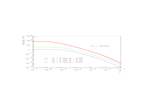
Figure 6: The differential neutrino-proton cross section as a function of $y$, the fraction of the neutrino energy deposited to the proton.

The differential cross section as a function of $y$, the energy fraction deposited from the neutrino to the nucleon, is presented in Fig. 6 for the neutrino energy $E_{\nu}=10$ EeV and three sets of parameters of the RS model.

In order to estimate an effective range of variable $y$ which contributes to the neutrino-nucleon cross section, we have calculated a quantity

$$\sigma^{\nu N}(y>y_{0})=\int\limits_{y_{0}}^{1}\frac{d\sigma^{\nu N}}{dy},$$ (29)

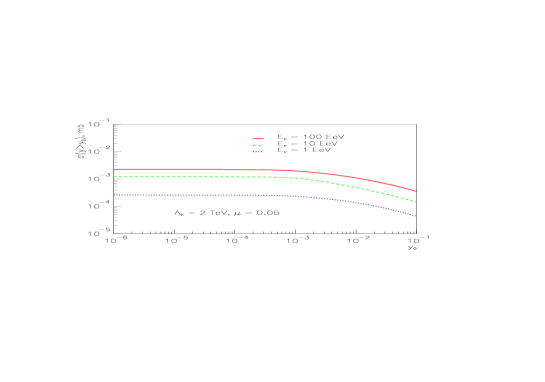
Figure 7: The inelastic neutrino-proton cross-section obtained by integrating the differential cross section in the region $y_{0}\leqslant y\leqslant 1$ as a function of $y_{0}$, the minimal fraction of the neutrino energy deposited to the proton.

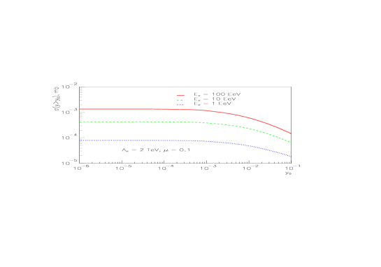
Figure 8: The same as in Fig. 7 but for the different value of $\mu=0.1$.

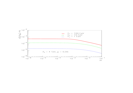
Figure 9: The same as in Fig. 7 but for the different value of $\Lambda_{\pi}=$ 4 TeV.

where $y_{0}$ is a minimum fraction of energy lost by the neutrino (deposited to the nucleon). The dependence of the quantity $\sigma_{el}(y>y_{0})$ on $y_{0}$ at different values of the neutrino energy $E_{\nu}$ is shown in Fig. 7 for $\Lambda_{\pi}=2$ TeV, $\mu=0.05$. Next two figures, Fig. 8 and Fig.  9, show the dependence of $\sigma_{el}(y>y_{0})$ on the parameters $\mu$ and $\Lambda_{\pi}$.

Ultra-high energy cosmic neutrinos have not yet been detected (see non-observation of neutrino-induced events reported by the Fly’s Eye [17], the AGASA [18] and the RICE [19] collaborations). A number of experiments under construction will allow to measure fluxes of such neutrinos within the next few years. Among them are Pierre Auger Observatory, IceCube neutrino telescope at the South Pole, Anita radio detector for a balloon flights around the South Pole, as well as EUSO, SalSA and OWL proposals. We will consider the first possibility [20].

The number of horizontal hadronic air showers with the energy $E_{sh}$ larger than a threshold energy $E_{th}$, initiated by neutrino-nucleon interactions, is given by

$$N_{sh} = TN_{A}\int\limits_{E_{th}}^{E_{max}}dE\,\Big{[}\sum_{i=e,\,\mu,\,\tau}\!\Phi_{\nu_{i}}(E)\int\limits_{0}^{1}dy\,\,\frac{d\sigma_{\nu N}^{grav}(E)}{dy}\,{\cal A}(yE)\,\theta(yE-E_{th})$$ (30)

$$+ \sum_{i=e,\,\mu,\,\tau}\!\Phi_{\nu_{i}}(E)\,\sigma_{\nu_{i}N}^{SM}(E)\,{\cal A}(\bar{y}_{i}E_{\nu_{i}})\,\theta(\bar{y}_{i}E-E_{th})\Big{]},$$

where $N_{A}=6.022\cdot 10^{23}\text{ g}^{-1}$, $T$ is a time interval (one year, in our case), and ${\cal A}(E)$ is a detector acceptance as a function of a shower energy (in units of km³ steradian water equivalent $=10^{15}$ g). The quantity $\Phi_{\nu_{i}}(E)$ in (30) is a flux of the neutrino of type $i$. Both neutrino and antineutrino are assumed in the sums in Eq. (30). The product $E\,\Phi_{\nu_{i}}(E)$ is in units of cm^-2 yr^-1. We have taken into account that the energy of the shower resulted from the gravitational interaction is equal to $yE$, and that this interaction is universal for all types of neutrinos.

For the energy distribution of the neutrino in the SM processes, we have used the approximation $d\sigma_{\nu_{i}N}^{SM}(y,E)/dy\simeq\sigma(E)\,\delta(y-\bar{y_{i}})$. The inelasticity $\bar{y}_{i}$ defines a mean fraction of the neutrino energy deposited into the shower in a corresponding SM process. We have put $\bar{y}_{e}=1$ for SM charged current interactions initiated by electronic neutrino, while for SM neutral interactions initiated by $\nu_{e}$ and for $\nu_{\mu}/\nu_{\tau}$-events we have taken $\bar{y}_{e}=\bar{y}_{\mu}=\bar{y}_{\tau}=0.2$ [21].

The number of extensive quasi-horizontal showers induced by so-called cosmogenic neutrinos which can be detected by the array of the southern site of the Pierre Auger Observatory, is presented in Table 1 for several sets of the RS parameters. These values of parameters are chosen in such a way in order not to violate experimental and theoretical bounds presented in Fig. 1. The cosmogenic neutrino flux is taken from Refs. [22], assuming $E_{max}=3\cdot 10^{21}$ eV. The acceptance of the Auger detector is taken from Ref. [23] (it is not assumed that a shower axis falls certainly in the array). The threshold energy $E_{th}$ is chosen to be $10^{17}$ eV.

For comparison, a SM background is presented in the last row of the Table 1. This value is in agreement with the number obtained recently for the same neutrino flux in Ref. [24].

Table 1: Yearly event rates for nearly horizontal neutrino induced showers with $\theta_{zenith}>70^{\circ}$ for the cosmogenic neutrino flux from Ref. [22] for three sets of the parameters. Number of events corresponds to one side of the Auger ground array.

	$\Lambda_{\pi}$=2 TeV, $\mu$=0.10	$\Lambda_{\pi}$=3 TeV, $\mu$=0.05	$\Lambda_{\pi}$=3 TeV, $\mu$=0.10
SM+grav	0.81	0.66	0.43
SM	0.24

The cosmogenic neutrino flux is the most reliable one, since it relies only on two assumptions: (i) the observed extremely high energy cosmic rays contain protons, (ii) these cosmic rays are primarily extragalactic in origin. Note, however, that the cosmogenic neutrino flux may be significantly depleted, if a substantial fraction of the cosmic ray primaries are heavy nuclei rather than protons [25].

The cosmogenic neutrino flux not only represents a lower limit on the flux of ultrahigh energy neutrinos, but it also can be used to put an upper limit on the neutrino flux. In Ref. [26] an upper limit (called WB bound) on a flux of neutrinos from compact sources which are optically thin to $p\gamma$ and $pp$ interactions (such as active galactic nuclei) has been obtained. The number of showers which can be registered by the Auger detector for this case is shown in Table 2. We have chosen the same threshold energy $E_{th}$ = 10¹⁷ eV and put $E_{max}=10^{21}$ eV.

Table 2: The same as in Table 1 but for the Waxman-Bahcall neutrino flux [26].

	$\Lambda_{\pi}$=2 TeV, $\mu$=0.10	$\Lambda_{\pi}$=3 TeV, $\mu$=0.05	$\Lambda_{\pi}$=3 TeV, $\mu$=0.10
SM+grav	1.03	0.78	0.49
SM	0.28

Note, the so-called cascade upper limit on transparent neutrino sources [27] (MPR bound) is 43 times higher that the WB bound. It exploits the EGRET data on the diffuse gamma-ray background [28].

The lower bound on the cosmogenic neutrino flux was also obtained under assumption that the observed extremely high energy cosmic rays below 10²⁰ eV are protons from uniformly distributed extragalactic sources [29]. It uses the fact that the proton are accumulated around the energy $E_{{}_{GZK}}=4\cdot 10^{19}$ eV due to the GZK mechanism [30]. The lower cosmogenic neutrino spectrum is practically cut at $E_{\nu}\simeq 2\cdot 10^{19}$ eV [29]. Other recent estimates of the cosmogenic neutrino fluxes can be found in Refs. [31, 24].

4 Conclusions and discussions

In the present paper we have calculated the contribution from the massive graviton modes to the eikonal in the RS model. The results were applied to the neutrino-nucleon scattering at transplanckian energies. Both differential and total cross sections are estimated for the different sets of the parameters of the model. By using differential cross sections, we have calculated the number of quasi-horizontal neutrino induced air showers which can be detected at the Auger Observatory per year. The estimates were obtained for two fluxes of cosmogenic neutrinos.

The differential cross section, $d\sigma(y)/dy$, where $y$ is the fraction of the neutrino energy $E_{\nu}$ deposited to the shower, can reach tens of mb at $y=0$, depending on energy (Fig. 6). However, the differential cross section exhibits a rapid fall-off in $y$, starting at some small $y$. As a result, the gravitational cross section appears to be approximately one order of magnitude larger than the SM cross section at the same energy. To illustrate this statement, let us fix the parameters of the RS model to be $\Lambda_{\pi}=2$ TeV, $\mu=0.1$. Then we have $(d\sigma(y)/dy)|_{y=0}\simeq 4$ mb for $E_{\nu}=10^{10}$ GeV (see Fig. 6). As one can see in Fig. 6, $d\sigma(y)/dy$ begins to fall rapidly at $y>10^{-5}$. The numerical calculations show that $\sigma\simeq 4\cdot 10^{-4}$ mb for this case (dashed curve in Fig. 8).

The energy of neutrino induced air shower, $E_{sh}=yE_{\nu}$, is bounded from below by a threshold energy $E_{th}$. Thus, the fraction $y$ should obey the inequality $y\geqslant E_{th}/E_{max}$, where $E_{max}$ is a maximum energy in a neutrino spectrum. For $E_{th}=10^{8}$ GeV and $E_{max}=10^{11(12)}$ GeV, we get $y\geqslant 10^{-3(4)}$. Thus, the air showers event rate is defined by the region of $y$, in which neutrino-nucleon cross section $d\sigma(y)/dy$ is significantly reduced in comparison with its magnitude at $y=0$. Nevertheless, gravity contribution to the event rate at the Auger detector is several times larger than the SM background, as one can see from Tables 1 and 2.

Recently, model independent bounds on the inelastic neutrino-nucleon cross section derived from the AGASA [18] and RICE [19] search results on neutrino events were obtained [24]. The bounds exploit the cosmogenic neutrino fluxes from Refs. [22, 29]. However, they were derived under an assumption that the total neutrino energy goes into shower energy, that is $y=1$. As we have seen, it is not a case for the gravitational interactions originated from $t$-channel KK gravitons, which prefer $y\ll 1$. Generally, in order to extract an upper limit on $\sigma_{tot}$, a dependence of $d\sigma(y)/dy$ on $y$ is needed. So, we conclude that the bounds from Ref. [24] can not be directly apply to the neutrino-nucleon cross sections derived in our scheme.

Appendix

In Appendix we calculate the dependence of the eikonal (20) on variable $u$ (19). Let us define

$$I(u)=\int\limits_{0}^{\infty}\,dx\,J_{0}(ux)\,R(x),$$ (A.1)

with

$$R(x)=\frac{I_{2}(x)}{I_{1}(x)}$$ (A.2)

being the ratio of two modified Bessel functions.

It easily to see from (A.1) that $I(u)\rightarrow u^{-1}$ at $u\rightarrow 0$, since $R(x)\rightarrow 1$ at $x\rightarrow\infty$. The asymptotics of $I(u)$ at large $u$ is defined by the behavior of the integrand at small $x$ which looks like

$$R(x)\simeq\frac{x}{4}-\frac{x^{3}}{96}+\frac{x^{5}}{1536}-\frac{x^{7}}{23040}+\mathrm{O}(x^{9}).$$ (A.3)

Let us now demonstrate that at $u\rightarrow\infty$ the function $I(u)$ (A.1) decreases faster that any fixed power of $u^{-1}$. By using well-known relation [32]

$$x^{\nu-1}J_{\nu-1}(ux)=\frac{1}{u}\,\Big{(}\frac{d}{x\,dx}\Big{)}\big{[}x^{\nu}J_{\nu}(ux)\big{]},$$ (A.4)

and integrating (A.1) by parts $k$ times, we obtain:

$$I(u)=\frac{1}{u^{k}}\int\limits_{0}^{\infty}\,dx\,J_{k}(ux)F_{k}(x),$$ (A.5)

where $J_{k}(z)$ is the Bessel function, and

$$F_{k}(x)=(-1)^{k}\,x^{k+1}\,\Big{(}\frac{d}{x\,dx}\Big{)}^{k}\left[\frac{R(x)}{x}\right].$$ (A.6)

The function $F_{k}(x)$ (A.6) has the following properties: it is proportional to $x^{k+1}$ at $x\rightarrow 0$, and it decreases as $x^{-k}$ at $x\rightarrow\infty$. For any positive integer $k$, it depends only on x and on the ratio $R(x)$ (A.2) (but not on $I_{1}(x)$ and $I_{2}(x)$ separately) due to the following relations between modified Bessel functions [32]:

$$\frac{d}{dx}I_{1}(x) = I_{2}(x)+\frac{1}{x}\,I_{1}(x),$$

$$\frac{d}{dx}I_{2}(x) = I_{1}(x)-\frac{2}{x}\,I_{2}(x).$$ (A.7)

For instance, for $k=1$ one has

$$F_{1}(x)=-1+\frac{4R(x)}{x}+\big{[}R(x)\big{]}^{2}$$ (A.8)

This expression has asymptotics $x^{2}/48$ and $x^{-1}$ at small and large $x$, respectively. For $k=2$ one gets

$$F_{2}(x)=\frac{1}{x}\Big{\{}-6\Big{[}1-\frac{4R(x)}{x}\Big{]}-2x\,R(x)+12\,\big{[}R(x)\big{]}^{2}+2x\,\big{[}R(x)\big{]}^{3}\Big{\}}$$ (A.9)

The asymptotics of $F_{2}(x)$ are $x^{3}/192$ and $3\,x^{-2}$.

Since $k$ is an arbitrary positive integer, we conclude from (A.5) and (A.6) that $\lim\limits_{u\rightarrow\infty}u^{a}\,I(u)=0$ for any $a>0$.

The integral in (A.5), contrary to an original one (A.1), converges rapidly at $x\rightarrow\infty$ for $k\geqslant 2$, and could be used for numerical calculations. It cannot be calculated analytically. However, there exists an expression which approximates our integral with a very high accuracy:

$$\bar{I}(u)=\int\limits_{0}^{\infty}\,dx\,J_{0}(ux)\,\bar{R}(x),$$ (A.10)

with

$$\bar{R}(x)=\frac{\sqrt{3}}{2}\,\frac{x}{\sqrt{x^{2}+12}}.$$ (A.11)

The function $\bar{R}(x)$ has the following expansion at $x^{2}<12$ (compare with Eq. (A.3)):

$$\bar{R}(x)\simeq\frac{x}{4}-\frac{x^{3}}{96}+\frac{x^{5}}{1536}-\frac{5\,x^{7}}{110592}+\mathrm{O}(x^{9}).$$ (A.12)

The integral (A.10) is a table one [33]:

$$\bar{I}(u)=\frac{\sqrt{3}}{2u}\,\exp(-2\sqrt{3}\,u).$$ (A.13)

We can integrate the RHS of (A.10) twice by parts,

$$\bar{I}(u)=\frac{1}{u^{2}}\int\limits_{0}^{\infty}\,dx\,J_{2}(ux)\,\bar{F}_{2}(x),$$ (A.14)

and compare $\bar{F}_{2}(x)=(3\sqrt{3}/2)\,x^{3}/(x^{2}+12)^{5/2}$ with the corresponding function $F_{2}(x)$ (A.9). The result of our calculations is presented in Fig. 10. Formula (A.13) gives practically the same dependence on variable $u$ as a numerical integration of the exact expression by using formula (A.5) (with $k=2$) does, see Fig. 11. Thus, $I(u)$ exhibits an exponential fall-off (as we expected, see above), and it becomes as small as $I(u)\simeq 0.01$ already at $u=1.2$.

Taking all said above into account, we put $I(u)\rightarrow\bar{I}(u)$, that results in the analytical expression for the eikonal presented in the text (21).

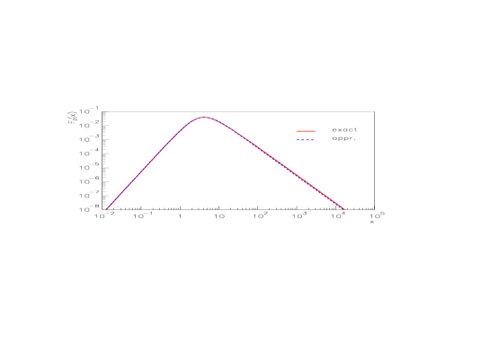
Figure 10: The exact integrand vs. approximate one (after the integration of both integrals by parts twice). See Appendix for details.

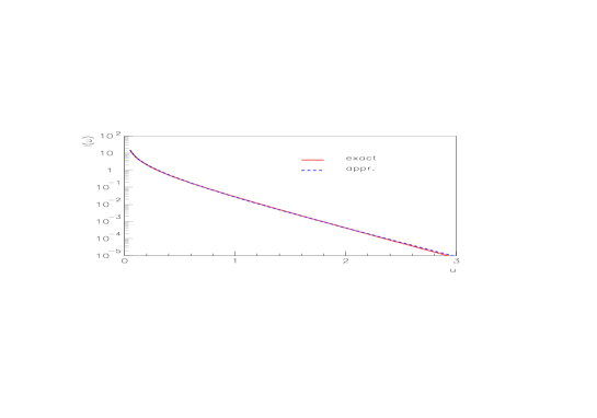
Figure 11: The input integral vs. approximate one as a function of the dimensionless variable $u$ (19). See Appendix for details.

References

- [1] L. Randall and R. Sundrum, Phys. Rev. Lett. 83 (1999) 3370.
- [2] L. Randall and R. Sundrum, Phys. Rev. Lett. 83 (1999) 4690; J. Lykken and L. Randall, JHEP 06 (2000) 014.
- [3] H. Davoudiasl, J.L. Hewett and T.G. Rizzo, Phys. Rev. D 63 (2001) 075004.
- [4] H. Davoudiasl, J.L. Hewett and T.G. Rizzo, Phys. Rev. Lett. 84 (2000) 2080.
- [5] B.C. Allanach et al., JHEP 0009 (2000) 019.
- [6] W.D. Goldberger and M.B. Wise, Phys. Rev. Lett. 83 (1999) 4922; C. Csáki et al., Phys. Rev. D 62 (2000) 045015; C. Csáki, M. Graesser and G.D. Kribs, ibid. D 63 (2001) 064020.
- [7] G.N. Watson, A Treatise on the Theory of Bessel Functions (McMillan, 1922).
- [8] T. Han, J.D. Lykken and R.-J. Zhang, Phys. Rev. D 59 (1999) 105006.
- [9] E. Dvergsnes, P. Osland and N. Öztürk, Phys. Rev. D 67 (2003) 074003.
- [10] G.F. Giudice, R. Rattazzi and J.D. Wells, Nucl. Phys. B 630 (2002) 293.
- [11] A.V. Kisselev, Eur. Phys. J. C 34 (2004) 513 .
- [12] G. ’t Hooft, Phys. Lett. B 198 (1987) 61; H. Verlinde and E. Verlinde, Nucl. Phys, B 371 (1992) 246; M. Fabbrichesi et al., Nucl. Phys. B 419 (1994) 174.
- [13] A.V. Kisselev and V.A. Petrov, Eur. Phys. J. C 36 (2004) 103; Eur. Phys. J. C 37 (2004) 241.
- [14] A.V. Kisselev and V.A. Petrov, in preparation.
- [15] V.A. Petrov, Proceedings of the Int. Conf. Theor. Phys., TH 2002 (Paris, July 2002, Eds. D. Iagolnitzer, V. Rivasseau and J. Zinn-Justin, Birkhäuser Verlag, 2003). Supplement (2003) 253.
- [16] S.I. Alekhin, Phys. Rev. D 68, 014002 (2003).
- [17] R.M. Baltrusaitis et al., Phys. Rev. D 31 (1985) 2192.
- [18] N. Inoue, Proc. 26th International Cosmic Ray Conference (ICRC 1999), eds. D. Kieda, M. Salamon and B. Dingus, Salt Lake city, Utah, 1999, v. 1, p. 361; S. Yoshida et al., Proc. 27th International Cosmic Ray Conference (ICRC 2001), Hamburg, Germany, 2001, v. 3, p. 1142
- [19] I. Kravchenko et al., Astropart. Phys. 20 (2003) 195; I. Kravchenko, arXiv: astro-ph/0306408.
- [20] Pierre Auger Observatory, http://www.auger.org/
- [21] G. Sigl, Phys. Rev. D 57, 3786 (1998).
- [22] R.J. Protheroe and P.A. Johnson, Astropart. Phys. 4, 253 (1996) [Erratum, ibid. 5, 215 (1996)]; R.J. Protheroe, Nucl. Proc. Suppl. 77, 465 (1999).
- [23] K.S. Capelle, J.W. Cronin, G. Parente and E. Zas, Astrophys. Phys.
- [24] L. Anchordoqui, Z. Fodor, S.D. Katz, A. Ringwald and H. Tu, arXiv: hep-ph/0410136.
- [25] D. Hooper, A. Taylor and S. Sarkar, arXiv: astro-ph/0407618.
- [26] J.N. Bahcall and E. Waxman, Phys. Rev. D 64 (2001) 023002.
- [27] K. Mannheim, R.J. Protheroe and J.P. Rachen, Phys. Rev. D 63 (2001) 023003.
- [28] P. Sreekumar et al., Astrophys. J. 494 (1998) 523.
- [29] Z. Fodor, S.D. Katz, A. Ringwald and H. Tu, JCAP 0311 (2003) 015; A. Ringwald, arXiv: hep-ph/0409151.
- [30] K. Greisen, Phys. Rev. Lett. 16 (1966) 748; G.T. Zatsepin and V.A. Kuzmin, JETP Lett. 4 (1966) 78.
- [31] O.E. Kalashev, V.A. Kuzmin, D.V. Semikoz and G. Sigl, Phys.Rev. D 66, 063004 (2002); D.V. Semikoz and G. Sigl, JCAP 0404 (2004) 003.
- [32] A. Erdelyi, W. Magnus, F. Oberhettinger and F.C. Tricomi (eds.), Higher Transcendental functions, v.2 (Mc Graw-Hill Book H. Company, 1955).
- [33] A.P. Prudnikov, Yu.A. Brychkov and O.I. Marichev, Integrals and series, v.2: Special functions, Translated from Russian (NY Gordon and Breach, 1986).
- [34] R. Emparan, M. Masip and R. Ratazzi, Phys. Rev. D 65 (2002) 064023.