The QCD phase diagram: A comparison of lattice and hadron resonance gas model calculations

Abstract

We compare the lattice results on QCD phase diagram for two and three flavors with the hadron resonance gas model (HRGM) calculations. Lines of constant energy density $\epsilon$ have been determined at different baryo-chemical potentials $\mu_{B}$. For the strangeness chemical potentials $\mu_{S}$, we use two models. In one model, we explicitly set $\mu_{S}=0$ for all temperatures and baryo-chemical potentials. This assignment is used in lattice calculations. In the other model, $\mu_{S}$ is calculated in dependence on $T$ and $\mu_{B}$ according to the condition of vanishing strangeness. We also derive an analytical expression for the dependence of $T_{c}$ on $\mu_{B}/T$ by applying Taylor expansion of $\epsilon$. In both cases, we compare HRGM results on $T_{c}-\mu_{B}$ diagram with the lattice calculations. The agreement is excellent, especially when the trigonometric function of $\epsilon$ is truncated up to the same order as done in lattice simulations. For studying the efficiency of the truncated Taylor expansion, we calculate the radius of convergence. For zero- and second-order radii, the agreement with lattice is convincing. Furthermore, we make predictions for QCD phase diagram for non-truncated expressions and physical masses. These predictions are to be confirmed by heavy-ion experiments and future lattice calculations with very small lattice spacing and physical quark masses.

I Introduction

The QCD phase diagram at finite temperatures and densities attracted increasing attention Rajagopal and Wilczek (2000), especially as it became possible to perform lattice QCD simulations at finite baryo-chemical potential $\mu_{B}$ Fodor and Katz (2002); de Forcrand and Philipsen (2002); Allton et al. (2002); D’Elia and Lombardo (2003). The numerical studies for the equation of state at finite $\mu_{B}$ provides a valuable framework for understanding the experimental signatures for the phase transition from confined hadrons to quark-gluon plasma (QGP). The heavy-ion experiments are aiming to explore the QCD phase diagram. Therefore, it is of great interest to show the interrelation between strangeness and baryo-chemical potentials and $T_{c}$ in hadron resonance gas model (HRGM) compared with the available lattice QCD simulations.

It is known that QCD phase diagram has a very rich structure. From numerical simulations, we know that the location of the phase transition line depends on the quark masses and flavors and the way of including the strange quark chemical potential $\mu_{s}$ at different values of $\mu_{B}$ and $T$. The isospin chemical potential can play an additional role. But relative to $\mu_{B}$ and $\mu_{s}$, the isospin chemical potential is very small, so that we can assume an entire symmetry in light quark potentials and therefore ignore the isospin chemical potential.

The first point in QCD phase diagram, namely the point at $T_{c}$ and $\mu=0$, has been a subject of different lattice simulations Fodor and Katz (2002); de Forcrand and Philipsen (2002); Allton et al. (2002); D’Elia and Lombardo (2003); Karsch et al. (2001); Karsch (2002); Gavai and Gupta (2003). We know so far that for two quark flavors ($n_{f}=2$) the transition is second order or rapid crossover and the critical temperature is $T_{c}\approx 173\pm 8\;$MeV. For $n_{f}=3$, we have a first order phase transition and $T_{c}\approx 154\pm 8\;$MeV. For $n_{f}=2+1$, i.e. two degenerate light quarks and one heavy strange quark, the transition is crossover and $T_{c}\approx 173\pm 8\;$MeV. For the pure gauge theory, $T_{c}\approx 271\pm 2\;$ MeV and the deconfinement phase transition is first order.

The lattice QCD simulations at $\mu_{B}\neq 0$ is still lacking an effective exact algorithm and suffer from the sign-problem. The fermion determinant gets complex and therefore the conventional Monte Carlo techniques are no longer applicable, since the lattice configurations can no longer be generated with the probability of the Boltzmann weight. However, during the last few years considerable progress has been made to overcome these problems Fodor and Katz (2002); de Forcrand and Philipsen (2002); Allton et al. (2002); D’Elia and Lombardo (2003).

The significant numerical results on positioning the QCD phase diagram we have so far is that the transition line can be described by a parabola. This simple relation can be viewed as a reflection of the truncations done in the Taylor expansions of different thermodynamic quantities calculated on lattice. In addition, we know from effective models such as bootstrap and Nambu-Jona-Lasinio models that the structure of the phase diagram is complex. The freeze-out curve takes a much different behavior at large chemical potential Tawfik (2004a, b). Nevertheless, one might think that for small chemical potential ($\mu_{q}\approx T_{c}$) the curvature of $T_{c}$-dependence upon $\mu_{q}$ can be fitted as a parabola, where $\mu_{q}$ is the quark baryo-chemical potential. The situation at very large chemical potentials is not clear. One might need to take into account other effects, such as quantum effects at low temperatures Miller and Tawfik (2003a, b, c, 2004a); Hamieh and Tawfik (2004); Miller and Tawfik (2004b), which might be able to describe the change in the correlations from confined hadrons to coupled quark-pairs.

In present work, we take advantage of our previous work Karsch et al. (2003a, b); Redlich et al. (2004) on analysis the critical temperatures $T_{c}$ for different quark masses and on reproducing the lattice thermodynamics at zero and finite $\mu_{B}$ by HRGM. We assumed that the deconfinement is driven by a constant energy density. We have shown Karsch et al. (2003a, b) that the degrees of freedom rapidly increase at $\epsilon_{c}(T_{c},\mu_{B}=0)$. Here, we assume that $\epsilon_{c}$ remains constant along the whole phase transition line Redlich et al. (2004); Toublan and Kogut (2004), $\epsilon_{c}(T_{c},0)=\epsilon_{c}(T_{c},\mu_{B})$. Concretely, we propose that the existence of different transitions does not affect the assumption that $\epsilon_{c}$ is constant for all $\mu_{B}$-values. We have to emphasize here that it is not possible in the framework of this model to make any statement about the transition at very large $\mu_{B}$ and low $T$. As $T\rightarrow T_{c}$, HRGM is no longer applicable. The nature of the degrees of freedom in this region is very different from that of the nearly non-interacting QGP at high $T$ and low $\mu_{B}$. The message we have in this paper is that the condition driving the QCD phase transition at finite $T$ and $\mu_{B}$ Karsch et al. (2003a, b); Redlich et al. (2004) is the energy density. Its value is not affected by the conjecture of existing of different transitions along the whole $\mu_{B}$-axis.

The model will be presented in Sec. II. In Sec. III, we introduce expressions for the lines of constant $T_{c}$. The lines of constant energy density are given in Sec. IV. The results are discussed in Sec. V. Sec. VI is devoted to the radius of convergence. In Sec. VII, we summarize the conclusions.

II The model

Assuming an ideal quantum gas consisting of point-like hadron resonances, the canonical partition function for one particle and its anti-particle reads

$${\cal Z}(V,T,\mu) = g\frac{V}{2\pi^{2}}\int_{0}^{\infty}dk\;k^{2}\left\{\ln(1\pm e^{-(\varepsilon-\mu)/T})+\ln(1\pm e^{-(\varepsilon+\mu)/T})\right\},\hskip 28.45274pt$$ (1)

where $\pm$ stand for bosons and fermions, respectively. $\varepsilon=(k^{2}+m^{2})^{1/2}$ is the single-particle energy and $g$ is the spin-isospin degeneracy factor. Under the given assumptions, one can sum up the contributions from all resonances pieces, so that

$$\ln{\cal Z}^{(id)}(V,T,\mu) = \sum_{i}^{\infty}\ln{\cal Z}_{i}(V,T,\mu_{i}).$$ (2)

In this expression, there are two important features included; the kinetic energies and the summation over all degrees of freedom and energies of resonances. On the other hand, we know that the formation of resonances can only be materialized through strong interactions Hagedorn (1965); Resonances (fireballs) are composed of further resonances (fireballs), which in turn consist of resonances (fireballs) and so on.

In spite of this, if one would like to take into consideration all kinds of resonance interactions in HRGM, then, for instance, by means of the $S$-matrix, we can re-write Eq. (2) as an expansion of the fugacity term.

$$\ln{\cal Z}^{(int)}(V,T,\mu) = \ln{\cal Z}^{(id)}(V,T,\mu)+\sum_{\nu=2}^{\infty}a_{\nu}(T)\exp(\mu_{\nu}/T).$$ (3)

$S$-matrix describes the scattering processes in the thermodynamical system Dashen et al. (1969). $a_{\nu}(T)$ are the so-called virial coefficients and the subscript $\nu$ refers to the order of the multiple-particle interactions.

$$a_{\nu}(T) = \frac{g_{r}}{2\pi^{3}}\int_{M_{\nu}}^{\infty}dw\;e^{-\varepsilon_{r}(w)/T}\;\sum_{l}(2l+1)\frac{\partial}{\partial w}\delta_{l}(w).$$ (4)

The sum runs over the spatial waves. The phase shift $\delta_{l}(w)$ of two-body inelastic interactions, for instance, depends on the resonance half-width $\Gamma_{r}$, spin and mass of produced resonances,

$$\ln{\cal Z}^{(int)}(V,T,\mu) = \ln{\cal Z}^{(id)}(V,T,\mu)+\frac{g_{r}}{2\pi^{3}}\int_{M_{\nu}}^{\infty}dw\frac{\Gamma_{r}\;e^{(-\varepsilon_{r}(w)+\mu_{r})/T}}{(M_{r}-w)^{2}+\left(\frac{\Gamma_{r}}{2}\right)^{2}}.\hskip 28.45274pt$$ (5)

By inserting $-\mu$ in place of $\mu$ in Eq. (5), we take into consideration the two-particle inelastic interactions, from which the anti-particles will be produced. For narrow width and/or at low $T$, the virial term reduces, so that we will get the non-relativistic ideal partition function of the hadron resonances with effective masses $M_{\nu}$. In other words, the resonance contributions to the partition function are the same as that of free particles with some effective mass. At temperatures comparable to $\Gamma_{r}$, the effective mass approaches the physical one. Thus, at high temperatures, the strong interactions are taken into consideration via including heavy resonances, Eq. (2). We therefore suggest to use the canonical partition function Eq. (2) without any corrections. Furthermore, we do not apply the excluded volume corrections. We include all hadron resonances with masses up to $2\;$GeV, such a way we avoid the singularities expected at Hagedorn temperature Karsch et al. (2003a, b).

In the two sections which follow, we discuss how to include the strangeness chemical potential $\mu_{S}$ in HRGM and lattice QCD.

II.1 $\mu_{s}$ in hadron resonance gas model

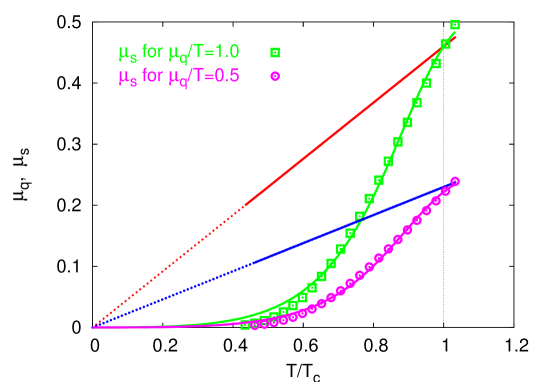
Fig. 1: The strange quark chemical potential $\mu_{s}$ vs. $T/T_{c}$ for $\mu_{q}/T=1$ and $\mu_{q}/T=0.5$ (straight lines). The results are fitted according to Eq. (9). At $T=0$, we find that $\mu_{q}=\mu_{s}=0$. As $T\rightarrow T_{c}$, the strangeness chemical potential approaches the baryo-chemical potential, $\mu_{s}=\mu_{q}$. The units used here are $\sqrt{\sigma}\sim 420\;$MeV.

The hadron-based chemical potentials $\mu_{B},\,\mu_{S}$ are related to the quark-based ones, $\mu_{q},\,\mu_{s}$

$$\mu_{B} = 3\,\mu_{q},\hskip 56.9055pt\mu_{S}=\mu_{q}-\mu_{s},$$ (6)

Assuming that the isospin and charge chemical potentials are vanishing, we use the following combination for the hadron resonances

$$\mu = 3b\mu_{q}+s\mu_{s},$$ (7)

where $b$ and $s$ are the baryon and strange quantum numbers, respectively. Obviously, this expression is valid for baryons as well as for mesons. The quantum numbers are entirely conserved.

The initial conditions in heavy-ion collisions apparently include zero net strangeness. This is expected to remain the case during the whole interaction unless an asymmetry in the production of strange particles happens during the hadronization. As we are interested in the hadron thermodynamics and location of QCD phase transition, we suppose that the net strangeness is entirely vanishing. The average strange particle number reads

$$<n_{s}> = \frac{1}{N}\sum_{i}^{N}\lambda^{(i)}_{s}\frac{\partial\ln{\cal Z}^{(i)}(V,T,\mu)}{\partial\lambda^{(i)}_{s}}.$$ (8)

$\ln{\cal Z}$ is given in Eq. (3) and $\mu_{S}$ is given in Eq. (6). $\lambda_{s}=\exp(\mu_{S}/T)$ is the fugacity factor of $s$ quark. The procedure used to calculate the quark-based $\mu_{s}$ is the following: For given $T$ and $\mu_{q}$ (or $\mu_{B}$), we iteratively increase $\mu_{s}$ and in each iteration, we calculate the difference $<n_{s}>-<n_{\bar{s}}>$, Eq. (8). The value of $\mu_{s}$ which disposes zero net strangeness is the one we read out and shall use in calculating the thermodynamic quantities. As in Eq. (6) the relation between $\mu_{s}$ and $\mu_{S}$ is given by taking into consideration the baryonic property of $s$ quark. The resulting $\mu_{s}$ for different $\mu_{q}$ (or $\mu_{B}$) and $T$ are depicted in Fig. 1. From this numerical method, we fit $\mu_{s}$ as a function of $T$ and $\mu_{B}$,

$$\mu_{s} \approx \frac{0.138\;\vartheta\;\theta^{3}}{1-2.4\;\theta^{2}+2.7\;\theta^{3}},$$ (9)

where $\vartheta\equiv\mu_{q}/T$ and $\theta\equiv T/T_{c}$.

Let us note here that for these calculations we have re-scaled the resonance masses in order to be comparable to the quark masses used in lattice QCD simulations. The procedure of giving unphysically heavy masses to the hadron resonances is introduced in Karsch et al. (2003a, b). In these calculations, the mass of lightest Goldstone meson becomes $m_{\pi}=770\;$MeV and consequently, the critical temperature gets almost as large as $200\;$MeV at $\mu_{B}=0$.

In order to guarantee vanishing net strange particle numbers in HRGM as the case in heavy-ion collisions, it is not enough to simply set $\mu_{s}=0$ and consequently, $\mu_{S}=\mu_{q}=\mu_{B}/3$ in Eq. (8). However, there are publications in which the authors have assigned $\mu_{s}$ to zero in hadron matter and afterwards applied the Gibbs condition for the first order phase transition to QGP. The reason is obvious. Aside the baryons, the strange mesons with different contents of $s$ quarks play determining roles at different temperatures and therefore, affect the final results, Eq. (6). Setting $\mu_{s}=0$, leads to violating the strange quantum numbers. Nevertheless, we will show here calculations in which we set $\mu_{s}=0$. We do this in order to extensively compare with lattice results. We apply this assignment in order to check the ability of HRGM in reproducing the current lattice simulations Toublan and Kogut (2004). After accomplishing this successfully, we can go beyond the lattice constrains to show the physical picture. We will make predictions for QCD phase diagram for physical masses and non-truncated Taylor series for thermodynamical expressions. These predictions are to be confirmed by heavy-ion experiments and future lattice calculations with very small lattice spacing and physical quark masses.

For completeness of the discussion, we recall the situation in the plasma regime (see also next section). For conserving strangeness at $T>T_{c}$, we have to suppose that $\mu_{S}=0$. $\mu_{S}$ consists of one baryonic part $\mu_{B}/3$ and another part coming from the strangeness quantum number $-\mu_{s}$. From Eq. (6), we then get

$$\mu_{s} = \mu_{q}=\mu_{B}/3.$$ (10)

This result is numerically confirmed in Fig. 1. For $\mu_{q}=0$ (or $\mu_{B}=0$), we find that $\mu_{s}=0$ for all temperatures. $\mu_{s}$ increases with increasing both $\mu_{q}$ and $T$. At $T_{c}$, we find that $\mu_{q}\approx\mu_{s}$. Therefore, we can suggest to set $\mu_{q}=\mu_{s}$ for all temperatures above $T_{c}$.

We can so far summarize that $\mu_{S}$ in the hadron matter has to be calculated in dependence on $\mu_{B}$ and $T$ under the assumption that the net strangeness is vanishing. In the QGP phase, one might fulfill this assumption by setting $\mu_{s}=\mu_{B}/3$. As we will see later, in lattice simulations, one assigns $\mu_{S}=\mu_{s}=0$. We deal with all these cases in this work.

II.2 $\mu_{s}$ in lattice QCD

In the Euclidian path integral formulation, the partition function of lattice QCD at finite $T$ and $\mu$ reads

$${\cal Z}(T,\mu) = \mbox{Tr}\;e^{-(H-\mu N)/T}$$ (11)

$$= \int{\cal D}\psi\;{\cal D}\bar{\psi}\;{\cal D}A\;e^{{\cal S}_{f}(V,T,\mu)+{\cal S}_{g}(V,T)},\hskip 28.45274pt$$

where $(\psi,\bar{\psi})$ and $A$ are the fermion and gauge fields, respectively. The chemical potential $\mu$ is given in Eq. (7). By Legendre transformation of the Hamiltonian $H$, we get the Euclidian action ${\cal S}=\int_{0}^{1/T}dt\int_{V}d^{3}x{\cal L}$. The fermionic action is

$${\cal S}_{f} = a^{3}\sum_{x}\left[ma\bar{\psi}_{x}\psi_{x}+\frac{1}{2}\sum_{k=1}^{4}\left(\bar{\psi}_{x}\gamma_{k}\psi_{x+\hat{k}}-\bar{\psi}_{x+\hat{k}}\gamma_{k}\psi_{x}\right)+\mu a\bar{\psi}_{x}\gamma_{4}\psi_{x}\right],\hskip 28.45274pt$$ (12)

where $a$ is the lattice spacing. As given in Eq. (8), the number density of the quarks with flavor number $x$ is obtained by derivation with respect to $\mu_{x}$,

$$n_{x}=\frac{\partial}{\partial\mu_{x}}\ln{\cal Z}(T,\mu_{x}).$$ (13)

For checking the dependence of $\mu_{s}$ on $\mu_{q}$ and consequently on $\mu_{B}$, it is enough to approximate the fermionic part of lattice QCD Lagrangian for three quark flavors as

$${\cal L} \approx \mu_{q}\left(\sum_{x\in\{u,d\}}\bar{\psi}_{x}\gamma_{4}\psi_{x}\right)+\mu_{s}\bar{\psi}_{s}\gamma_{4}\psi_{s}$$ (14)

$$\approx \hskip 5.69054pt\mu_{q}n_{u}+\mu_{q}n_{d}+\mu_{s}n_{s}.$$

To taken into account the conservation of the baryon and strange quantum numbers, the summation in last expression has to run over $s$ quarks, too. By doing this, last term turns to be $(\mu_{q}-\mu_{s})\,n_{s}$. Then we expect that the strangeness on lattice vanishes at $\mu_{s}=\mu_{q}$. But from Eq. (14), which reflects the situation in current lattice simulations, we find that $n_{s}=0$ for $\mu_{s}=0$.

As discussed in previous section, the strangeness in QGP is conserved at $\mu_{s}=\mu_{q}=\mu_{B}/3$. In the hadron regime, especially at large $\mu_{B}$, $\mu_{s}$ (or $\mu_{S}$) has to be calculated as a function of $T$ and $\mu_{B}$ (Fig. 1). In spite of these considerations, the reliable lattice QCD simulations are still limited to $\mu_{B}\approx 3T_{c}$. As we will see in Sec. V, at this small value, there is practically no big difference between $\mu_{s}=0$ and $\mu_{s}=f(T,\mu_{B})$.

III Lines of constant $T_{c}$

III.1 $T_{c}(\mu)$ in hadron resonance gas model

In Boltzmann limit, the energy density in an ideal quantum system consisting of one particle and its anti-particle can be expressed as

$$\epsilon(T,\mu) = \frac{g}{\pi^{2}}Tm^{2}\left[mK_{1}\left(\frac{m}{T}\right)+3TK_{2}\left(\frac{m}{T}\right)\right]\cosh\left(\frac{\mu}{T}\right).$$ (15)

$\mu$ is given in Eq. (7). We can divide this expression into two sectors: one meson- $m$ and one baryon-sector $b$ Karsch et al. (2003b); Karsch (2004),

$$\varepsilon_{h}(T,\mu) = \varepsilon_{m}(T)+\varepsilon_{b}(T)\;\cosh(\mu/T).$$ (16)

Applying truncations in the Taylor expansions of $\cosh(\mu/T)$ up to the second order of $\mu/T$ - as done in lattice calculations Ejiri et al. (2004) - we can estimate the lines of constant $T_{c}$ in HRGM. In doing this, we assume that $\varepsilon_{h}(T,\mu)=\varepsilon_{h}(T_{c},0)$. Furthermore, we assume that the dependence of energy density on the quark mass is quite small. We see this in Fig. 2 which is reported in Ref. Ali Khan et al. (2001). At $T_{c}$ and for the same temporal lattice dimension $N_{\tau}$, there is very small change in $\varepsilon_{c}$ for different quark masses. The latter are related to the pion masses via $m_{\pi}^{2}\propto m_{q}$.

The starting point in expressing $T_{c}(\mu_{B})$ for constant ratios $\mu_{B}/T$ is to expand Eq. (16) around the points $T=T_{c}$ and $\mu_{B}=0$. The second-order expansion gives

$$\varepsilon_{h}(T,\mu_{B}) = \varepsilon_{h}(T_{c},0)+\left[\frac{\partial\varepsilon_{h}(T_{c},0)}{\partial T}(T-T_{c})+\frac{1}{2}\mu_{B}^{2}\frac{\partial^{2}\varepsilon_{b}(T_{c},0)}{\partial\mu_{B}^{2}}\right],$$ (17)

$$= \varepsilon_{h}(T_{c},0)+\left[\frac{\partial\varepsilon_{h}(T_{c},0)}{\partial T}(T-T_{c})+\frac{1}{2}\varepsilon_{b}(T_{c},0)\left(\frac{\mu_{B}}{T}\right)^{2}\right].$$

Under the assumptions given above, this leads to the following parabola:

$$\frac{T_{c}(\mu_{B})}{T_{c}(\mu_{B}=0)} = 1-\frac{9}{2}\frac{1}{T_{c}(\mu_{B}=0)}\left[\frac{\varepsilon_{b}(T_{c},0)}{\frac{\partial}{\partial T}\varepsilon_{h}(T_{c},0)}\right]\left(\frac{\mu_{q}}{T}\right)^{2},$$ (18)

where $\mu_{q}=\mu_{B}/3$. In order to map out the QCD phase diagram by using this analytic expression, we merely need to calculate the baryon energy density $\epsilon_{b}$ at $T_{c}$ and $\mu_{q}=0$ and the derivative of the hadron energy density with respect to $T$, $\partial\varepsilon_{h}(T_{c},0)/\partial T$. The results are given in Sec. V. Evidently, it is possible to extend the above expression to include further higher terms of $\mu_{q}/T$.

Then to determine $T_{c}$ at given $\mu_{B}$, we apply besides the above analytical method the condition of constant critical energy density Redlich et al. (2004); Toublan and Kogut (2004) (see Sec. IV). In this case, $T_{c}$ is defined as the temperature at which the energy density in HRGM reaches a certain critical value. This value can be taken from lattice QCD simulations at $\mu_{B}=0$.

III.2 $T_{c}(\mu)$ in lattice QCD

In lattice QCD simulations, the critical temperature $T_{c}(\mu)$ is to be calculated from the pseudo-critical coupling $\beta_{c}(\mu)$ by determining the susceptibility peak in either the Polyakov loop or the chiral condensate in $\beta-\mu$ dimensions. The lattice beta function $\beta(a)$ which can be obtained from the string tension is needed in order to express the results in physical units. From the first non-trivial Taylor coefficients of $T_{c}(\mu)$, we get

$$\frac{d^{2}}{d\mu^{2}}T_{c}(\mu) = -\frac{N_{\tau}^{-2}}{T_{c}(\mu=0)}\frac{\partial^{2}\beta_{c}(\mu)}{\partial\mu^{2}}\left(a^{-1}\frac{\partial a}{\partial\beta}\right),$$ (19)

where $N_{\tau}$ is the temporal lattice dimension.

In the lattice QCD simulations Allton et al. (2002) with $n_{f}=2$ and quark mass $am_{q}=0.1$, the dependence of $T_{c}$ on $\mu_{q}$ has been found to take the following (parabola) expression:

$$\frac{T_{c}(\mu_{q})}{T_{c}(\mu_{q}=0)} = 1-0.070(35)\left(\frac{\mu_{q}}{T_{c}(\mu_{q}=0)}\right)^{2}.$$ (20)

In other lattice QCD simulations with the same flavor number but quark masses four times heavier than the physical masses de Forcrand and Philipsen (2002),

$$\frac{T_{c}(\mu_{q})}{T_{c}(\mu_{q}=0)} = 1-0.050(34)\left(\frac{\mu_{q}}{T_{c}(\mu_{q}=0)}\right)^{2}.$$ (21)

It has been concluded Allton et al. (2002) that the last relation remains almost unchanged for $am_{q}=0.005$. In this regard, we have to remember that for small quark masses perturbative beta function has been used. As we will see later, we actually find an increase in the curvature with reducing resonance masses from the values which very well simulate the current lattice calculations ($m_{\pi}\approx 770\;$MeV) to the physical masses, at which the lightest Goldstone meson is the physical pion ($m_{\pi}=140\;$MeV).

The results from Eq. (20) are depicted in Fig. 3. In the same figure, we plot Eq. (21). We also plot other lattice results Allton et al. (2002), namely the short vertical lines which give $T_{c}$ at constant energy density.

$n_{f}=3$ lattice QCD results Karsch et al. (2004) for different quark masses obtained so far can be summarized as

$$\frac{T_{c}(\mu_{q})}{T_{c}(\mu_{q}=0)} = 1-0.025(6)\left(\frac{\mu_{q}}{T_{c}(\mu_{q}=0)}\right)^{2},\hskip 28.45274ptam_{q}=0.1,$$ (22)

$$= 1-0.114(46)\left(\frac{\mu_{q}}{T_{c}(\mu_{q}=0)}\right)^{2},\hskip 22.76219ptam_{q}=0.005.$$ (23)

Again, in these simulations the beta function for the small quark masses has been calculated perturbatively. The results from these two expressions are depicted in Fig. 5 and Fig. 6, respectively. From other $n_{f}=3$ lattice QCD simulations de Forcrand and Philipsen (2003),

$$\frac{T_{c}(\mu_{q})}{T_{c}(\mu_{q}=0)} = 1-0.0610(90)\left(\frac{\mu_{q}}{T}\right)^{2}+0.00235(89)\left(\frac{\mu_{q}}{T}\right)^{4}.\hskip 17.07164pt$$ (24)

The curvature from $n_{f}=2+1$ lattice simulations Fodor (2003) has been compared with the three flavor one de Forcrand and Philipsen (2002) and concluded that there is a complete agreement. As we will see in Fig. 6, the most recent $n_{f}=2+1$ lattice simulations of Fodor and Katz (2004) result in a curvature smaller than those from other lattice simulations. This can be understood according to the different fermionic actions used.

IV Lines of constant energy density

In previous work Redlich et al. (2004), we have used HRGM in order to determine $T_{c}$ corresponding to a wide range of quark (pion) masses at $\mu_{B}=0$. The masses range from the chiral to pure gauge limits. We have seen that the condition of constant energy density can excellently reproduce the critical temperature $T_{c}$ as a function of $m_{q}$ and $n_{f}$. In present work, we extend this condition to finite chemical potentials $\mu_{B}$. We use two models for including the strangeness chemical potential $\mu_{S}$. In the first model, we calculate $\mu_{S}$ in dependence on $\mu_{B}$ and $T$ according to the condition of zero net strangeness. In the other one, we explicitly set the quark-based $\mu_{s}=0$. The last case is used in lattice QCD simulations. As given in Sec. II.2, the proper inclusion of $\mu_{s}$ in QGP and in lattice Lagrangian is to assign to it the same value of $\mu_{B}/3$. Nevertheless, both choices can be accepted for the current lattice QCD simulations, since the most reliable lattice calculations are currently performed at small baryo-chemical potentials ($\mu_{q}\approx T_{c}$). Consequently, the strangeness chemical potential is expected to be much smaller or at lest as small as the baryo-chemical potential.

As discussed above, in HRGM, the energy density at finite chemical potential can be divided into two parts: one from the meson sector and another one from the baryon sector. For the first part, we can completely drop out the fugacity term. For symmetric numbers of light quarks, the baryo-chemical potential of mesons is vanishing. But for strange mesons the strangeness chemical potential assigned to their $s$ quarks should be taken into account. For the baryon sector, the chemical potential is given by Eq. (7).

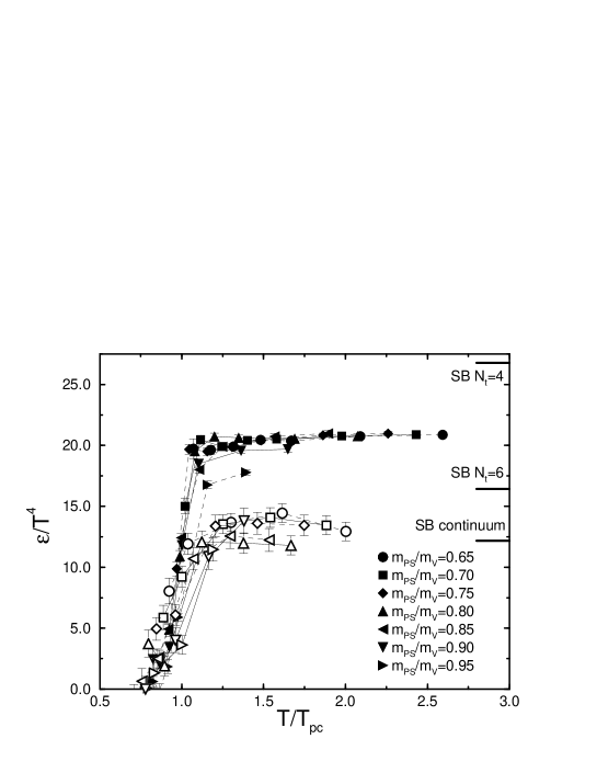
Fig. 2: The energy density normalized to $T^{4}$ given in dependence on $T/T_{c}$ for different quark masses $m_{q}$ and temporal lattice dimensions $N_{\tau}$. This figure is reported in Ref. Ali Khan et al. (2001).

The question we intent to answer is: which value has to be assigned to the critical energy density at finite chemical potentials? We recall the lattice QCD simulations. In Fig. 2, we see that the energy density  at $T_{c}$ is not a singular function but can rather be defined at different critical values depending on $n_{f}$ and $m_{q}$. This reflects the nature of the phase transition, cross-over. On the other hand, the uncertainty in calculating the energy density on lattice is very large, almost a factor $2$. The reason for this is the uncertainty in estimating $T_{c}$, Eq. (20). As mentioned above, $T_{c}$ is determined according to maximum susceptibility. The uncertainty in this quasi $T_{c}$ is $\sim 10\%$. The coefficients of $T$ have additional $\sim 20\%$.

The critical energy density at which we define $T_{c}(\mu_{B})$ in HRGM is taken from lattice QCD simulations at $\mu_{B}=0$ Karsch et al. (2001). In lattice units, the dimensionless energy densities for $n_{f}=2$ and $2+1$ are $\varepsilon/T^{4}|_{T_{c}}\cong 4.5\pm 2$ and $\cong 6.5\pm 2$, respectively. We take an average value and express it in physical units. Thus, $\epsilon_{c}=600\pm 300\;$MeV$/$fm³.

As in Allton et al. (2002), we assume that this value remains constant along the phase transition line; $\mu_{B}$-axis. The existence of different phase transitions (cross-over and first-order) and the critical endpoint, at which the transition is second-order, is assumed not to affect this assumption. As mentioned in Sect. III.2, the phase transition line on lattice is to be estimated according Eq. (19), i.e. up to $(\mu/T)^{2}$. Additional to this method, the line of constant energy density has been calculated Allton et al. (2002). By comparing the two lines, it has been found that they are almost coincident. In other words, the constant $\epsilon_{c}$ can be used to estimate the critical line at finite $\mu_{B}$. We have to remember that the lattice estimation of $\epsilon$ has a very large uncertainty, $\epsilon\propto T^{4}$. Therefore, the transition line according to constant $\epsilon_{c}$ has a larger uncertainty, because of the additional uncertainty in the derivatives of $\epsilon_{c}$ with respect to $\mu_{B}$ and $\mu_{B}^{2}$.

What are the consequences if the assumption of constant $\epsilon_{c}(\mu_{B})$ disregarding the uncertainty turned out to be incorrect? To discuss such consequences, we first recall the second-law of thermodynamics.

$$\partial\epsilon = T\,\partial s-p+\mu_{B}\,\partial n_{B},$$ (25)

where $s$, $p$ and $n_{B}$ are the entropy, the pressure and the baryon number density, respectively.

If $\epsilon_{c}$ were a decreasing function of $\mu_{B}$, this means that low incident energies are much more suitable to produce the phase transition from confined hadrons to deconfined QGP than the high incident energies! But the low limit should be given by the freeze-out curve Tawfik (2004b), i.e., the hadronization phase diagram. We know from phenomenological observations that both freeze-out curve and phase transition line are coincident at low $\mu_{B}$ (high incident energy). For large $\mu_{B}$ the two lines are separated. The freeze-out curve Tawfik (2004b) is given by $s/T^{3}=7$, entropy driven. Then along freeze-out curve it is expected that $\epsilon$ slightly increase with $\mu_{B}$. This means the assumption that $\epsilon_{c}$ decreases with increasing $\mu_{B}$ will give a phase transition which has $T_{c}$ much smaller than the freeze-out temperature.

In the other case, that $\epsilon_{c}$ increases with increasing $\mu_{B}$, we expect the $\epsilon_{c}$ required for the phase transition gets larger with decreasing the incident energy! According to Eq. (25), the phase diagram is given by $T_{c}=\partial\epsilon/\partial s$ at constant $n_{B}$ and $\mu_{B}=\partial\epsilon/\partial n_{B}$ at constant $T$. Then for increasing $\epsilon_{c}(\mu_{B})$, the critical temperature is expected to increase or at least remain constant. This result has the conconsequences that the phase transition at large $\mu_{B}$ will be diffecult to materialize in heavy-ion collisions or impossible. Also the phases of coupled quark-pairs (color superconductivity) will be expected for very large $\mu_{B}$ or not allowed at all.

Since we use constant $\epsilon_{c}$ down to low temperatures, one might ask if there could be any relation between $\epsilon_{c}$ and the experimental value of nuclear density. Obvioulsy at $T=0$, HRGM, Eq. (1), is no longer applicable. In this limit, we suppose that the hadron gas is composed of degenerate Fermi gas of nucleons. We can therefore calculate $\mu_{B}$ corresponding to the normal nuclear density at $T=0$ Tawfik (2004b). The value is $979\,$MeV. The energy density in this limit reads

$$\epsilon(\mu_{B}) = \frac{3\,g}{4\pi^{2}}\,m^{4}\;\left[\frac{\mu_{B}}{m}\sqrt{\frac{\mu_{B}^{2}}{m^{2}}-1}\left(\frac{\mu_{B}^{2}}{m^{2}}-\frac{1}{2}\right)-\frac{\ln\left(\frac{\mu_{B}}{m}+\sqrt{\frac{\mu_{B}^{2}}{m^{2}}-1}\right)}{2}\right]$$ (26)

V The results

Since we want to compare HRGM with lattice results de Forcrand and Philipsen (2002); Allton et al. (2002), some details about the lattice simulations at $\mu_{q}\neq 0$ are in order. Extensive details about HRGM are presented in Refs. Karsch et al. (2003a, b); Redlich et al. (2004). In order to avoid the sign problem in lattice simulations Allton et al. (2002), the derivatives of thermodynamic quantities with respect to $\mu_{B}=0$ at the point $T_{c}$ are first computed and then their Taylor expansion coefficients in terms of finite $\mu_{q}$ are calculated. The curvatures according to $T_{c}(\mu_{B})$ and $\epsilon_{c}(\mu_{B})$ are derived for different $m_{q}$. For instance for $am_{q}=0.1$, the corresponding pion mass in lattice units for $n_{f}=2$ is $am_{\pi}=0.958(2)$, where $a\sigma=0.271(10)$ Karsch et al. (2001). This leads to $m_{\pi}\cong 773\;$MeV. Keeping these features in mind, we performed our calculations for physical and re-scaled resonance masses. In Fig. 3, we find that our results are coincide with the lattice ones. In Ref. de Forcrand and Philipsen (2002), the lattice simulations are performed with an imaginary chemical potential for $n_{f}=2$ staggered quarks. For $\mu=i\mu_{I}$, the sign problem is obviously no longer existing. Using analytic continuation of the truncated Taylor series, one can then go to real $\mu$. The light quark mass is four times the physical mass. The location of $T_{c}$ at $\mu_{B}=0$ has been extrapolated to the chiral limit. The lattice results are represented by the short curves in Figs. 3, 4 and 6.

V.1 Results for two flavors

From the canonical partition function Eq. (1), we can derive the energy density at finite chemical potential $\mu\neq 0$ as

$$\epsilon(T,\mu) = T\frac{\partial T\ln{\cal Z}(T,\mu)}{\partial T}-T\ln{\cal Z}(T,\mu)+\mu\frac{\partial T\ln{\cal Z}(T,\mu)}{\partial\mu}\hskip 14.22636pt$$ (27)

$$= \frac{g}{2\pi^{2}}\;\int_{0}^{\infty}k^{2}\;dk\;\frac{\varepsilon(k)}{e^{[\varepsilon(k)-\mu]/T}\pm 1}.\hskip 22.76219pt$$

In Boltzmann limit and by taking into consideration only one particle and its anti-particle, we get the expression given in Eq. (15). It is obvious that the trigonometric function included in last expression are not truncated. In calculating this quantity in HRGM, we sum up over all resonances we take into account.

We first start with two flavors. It is not needed to care about the strangeness chemical potential. As discussed above, there are two lattice QCD simulations for $n_{f}=2$. In the first one, re-weighting methods, the physical quantities which usually can be calculated at $\mu_{B}=0$ without any difficulties have responses at finite $\mu_{B}$. The responses are utilized to estimate the thermodynamic quantities at finite $\mu_{B}$. The other lattice simulations de Forcrand and Philipsen (2002) use imaginary $\mu_{B}$ and afterwards apply analytical continuation. At given $\mu_{B}$, $T_{c}$ is determined as the temperature at which the energy density $\epsilon$ equals $600\;$MeV$/$fm³.

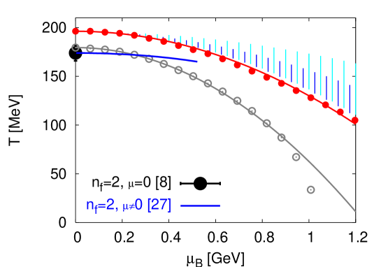
Fig. 3: $T-\mu_{B}$ phase diagram for two quark flavors $n_{f}=2$. The vertical lines give the lattice results Allton et al. (2002). The short lines show the results according to a constant $\epsilon_{c}$. The long ones are for constant $T_{c}$. The Lattice simulations are performed for large quark mass. The corresponding Goldstone pion gets a mass of $770\;$MeV. The solid circles give our results heavy quark masses. The results for physical quark masses are given by the open circles.

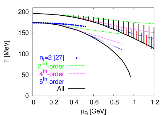
Fig. 4: The same as in Fig. 3. Here, we show the results obtained from the condition of constant $\epsilon_{c}$ truncated up the different Taylor orders. The truncation is obviously able to describe the lattice QCD simulations for different quark masses Allton et al. (2002); de Forcrand and Philipsen (2003). The solid lines give our predictions for non-truncated trigonometric functions.

The results are plotted in Fig. 3. The solid circles represent the results for re-scaled resonance masses. The open circles represent the results for physical masses. The two lines connecting the points are obtained by fits according to:

$$\frac{T_{c}(\mu_{q})}{T_{c}(\mu_{q}=0)} = 1-c_{1}\left(\frac{\mu_{q}}{T_{c}(\mu_{q}=0)}\right)^{2}.$$ (28)

The $\mu_{q}$-values are restricted within the range $0\leq\mu_{q}\leq T_{c}$. $\mu_{q}$ is given in Eq. (6). For the re-scaled heavy masses, the fit parameters are $c_{1}=0.115(36)$ and $T_{c}(\mu_{B}=0)=196.3\;$MeV. Plugging these parameters in Eq. (28), we get the top line in Fig. 3. The comparison with the lattice calculations Eq. (20) gives a satisfactory agreement, especially at low $\mu_{B}$. Nevertheless, it is obvious that our results at large $\mu_{B}$ lie below the lattice ones. The reason for this discrepancy will be discussed later.

One might ask whether the pion gas with very heavy masses would be able to describe the lattice results? To answer this question, we refer to Karsch et al. (2003b, a). In order to simulate the lattice QCD thermodynamiscs, for instance the rapid increase in $\epsilon$ near $T_{c}$, we need to include the corresponding degrees of freedom in HRGM. A hadron gas of pions can reproduce $\sim 15\%$ of the lattice QCD thermodynamiscs. Including heavier resonances gives the correct QCD thermodynamics. Furthermore, for lattice calculations with very heavy quark masses (pure gauge) we need to include the low-lying glueballs Karsch et al. (2003b).

As given above, the coefficient in the front of $(\mu_{q}/T)^{2}$ in Eq. (18) can be calculated in HRGM. For non-strange hadron resonances with re-scaled masses, the coefficient gets the value $0.0767$. Comparing to Eq. (20), this value is obviously much better than the value of $c_{1}$ in describing the lattice results. As we will see, this discrepancy is to be related to the fact that $c_{1}$ has been calculated from fitting $T_{c}$ at finite $\mu_{B}$ in the results which we have obtained from non-truncated $\epsilon(T,\mu_{B})$. We should emphasize that all Taylor terms that are higher than the second one are explicitly excluded in deriving Eq. (18). This partially explains the disagreement between HRGM and lattice results shown so far. We also study the case for physical resonance masses. The fit parameters are $c_{1}=0.195(21)$ and $T_{c}(\mu=0)=175\;$MeV. The coefficient in Eq. (18) is found to be $0.1368$.

In the following, we confront the lattice results with HRGM results which have been obtained from truncated expressions. We show the results in Fig. 4. We start with results from entire Taylor expansion for heavy resonance masses (solid line). This is equivalent to use Eq. (15) instead of Eq. (27). We note that this line shows almost the same behavior as that of the solid circles in Fig. 3. In deriving Eq. (15), the Boltzmann limit is assumed. The results from different truncations are also plotted. We find that the energy density truncated up to the second or fourth order of $\mu/T$ can describe the lattice results better than the solid line. The agreement between the curvatures of these two lines and that from the analytical expression Eq. (18) is excellent. The ability of truncated expression to produce results comparable to the lattice ones is to be explained by the fact that the lattice results themselves have been obtained from truncated thermodynamic expressions.

We plot in the same figure the HRGM results with physical masses. The curves obtained from different truncation terms in Eq. (15) represent our predictions when it will be possible to perform lattice simulations for two quark flavors with physical masses. These predictions has to be checked by future lattice simulations. We note that the solid line is comparable to the bottom points plotted in Fig. 3. The quark masses used in Ref. de Forcrand and Philipsen (2003) are relative heavy. Nevertheless, we see that the second order (dashed line) agrees very well with these lattice results de Forcrand and Philipsen (2003) (solid circles).

V.2 Results for three flavors

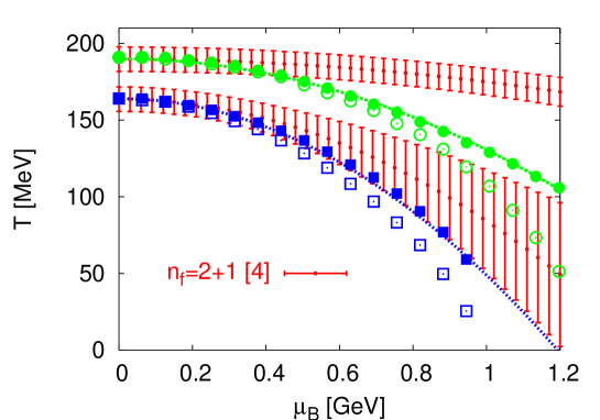
Fig. 5: The $T-\mu_{B}$ phase diagram for $n_{f}=3$. The vertical short lines represent the lattice results Allton et al. (2002). The above band corresponds to heavy quark masses. The bottom one is for physical masses. The solid circles are our results for heavy resonances and for $\mu_{s}=0$. The open circles are for $\mu_{s}=f(\mu_{B},T)$. The squares give the results for the physical masses. The curves are fitted according to Eq. (28).

We have to include strangeness chemical potential $\mu_{S}$ (Sec. II.1). Assuming that the three quarks are degenerate, we can use the same critical energy density as done in previous section. The results are shown in Fig. 5. The solid circles show the results for re-scaled heavy resonance masses. As done in lattice calculations, we first set $\mu_{s}=0$. The resulting points (solid circles) are fitted within the range $0\leq\mu_{q}\leq T_{c}$ according to Eq. (28). The fit parameters are $T_{c}=190\;$MeV and $c_{1}=0.1016$. The coefficient in front of $(\mu/T)^{2}$ in Eq. (18) is $0.0505$. Comparing with Eq. (22), this value can describe the lattice curvature much better than $c_{1}$. We also calculate $\mu_{s}$ in dependence on $\mu_{B}$ and $T$ assuming strangeness conservation. The open circles show the $T_{c}-\mu_{B}$ diagram corresponding to this value of $\mu_{s}$. We note that the former case ($\mu_{s}=0$) is much closer to the lattice results than the latter one. The reason is, as we mentioned above, that $\mu_{s}$ in lattice calculations used to be assigned to zero.

The results for physical masses are also shown in Fig. 5. The solid squares represent the results at $\mu_{s}=0$. These points are fitted according Eq. (28). The fit parameters are $T_{c}=164\;$MeV and $c_{1}=0.17$. The coefficient in Eq. (18) takes the value $0.1122$, which agrees very well with Eq. (23). The open squares represent the results at $\mu_{s}$ that depends on $\mu_{B}$ and $T$. The results with re-scaled resonance masses are given as circles. For $\mu_{s}=0$, we get results closer to lattice results than for $\mu_{s}=f(T,\mu_{B})$. In this figure, the energy density is calculated according to Eq. (27). In other words, the results plotted here are deduced from expression like Eq. (15), i.e. without any truncations.

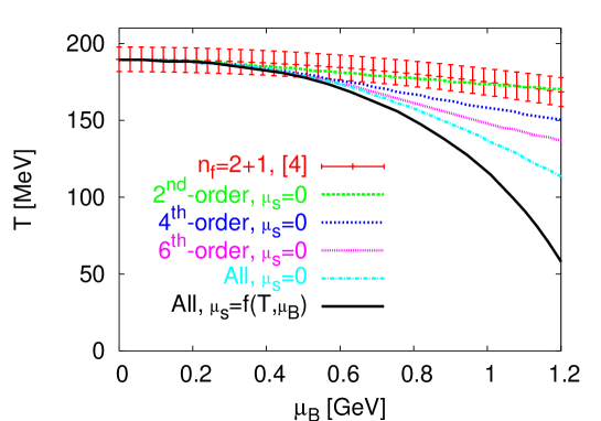
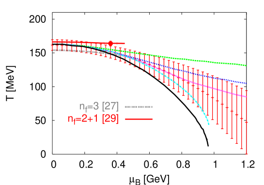
Fig. 6: $T-\mu_{B}$ phase diagram as in Fig. 5. Here, we check the effects of truncated trigonometric functions. The top panel shows the results for heavy masses. Truncating $\epsilon(T,\mu_{B})$ up to second order reproduces the lattice results Allton et al. (2002). In the bottom panel we show the results with physical masses. the lattice results Allton et al. (2002) are very well reproduced by the condition of constant truncated $\epsilon$. The results from non-truncated $\epsilon$ at $\mu_{s}=0$ and $\mu_{s}=f(T,\mu_{B})$ are also plotted, the bottom curves, respectively. The agreement with the lattice simulations de Forcrand and Philipsen (2003); Fodor and Katz (2004) is also convincing

We plot in Fig. 6 the results from different truncations, in order to compare HRGM results with lattice simulations. For heavy masses the results are given in the top panel. The results for physical masses are given in the bottom panel. It is clear that the truncation up to the second order gives results in a good agreement with the lattice simulations Allton et al. (2002). With higher truncations, we get curves with larger curvatures. We also plot two curves from non-truncated expressions for the trigonometric functions. The solid curve is obtained by computing $\mu_{s}$ in dependence on $T$ and $\mu_{B}$. Obviously, it is identical to the solid symbols plotted in Fig. 5. The dashed curve - next to the solid one - shows the results in which $\mu_{s}$ is entirely vanishing. It gives the same behavior as that of the open symbols in Fig. 5.

We can so far conclude that the lattice results Allton et al. (2002) can be reproduced by HRGM, if the trigonometric functions are truncated in the same way. The lattice curvature within the region $0\leq\mu_{q}\leq T_{c}$ can excellently be described by HRGM.

In the bottom panel, we show other three flavor lattice results. In Ref. de Forcrand and Philipsen (2003), the numerical simulations have been performed with Wilson gauge action and three degenerate flavors of staggered fermions. The quark masses are ranging between $0.025\leq am_{q}\leq 0.04$. It is clear that our results can reproduce the structure given by these data. We see that the curvature can be described by second or fourth order in HRGM. This is also valid for $n_{f}=2+1$ lattice results Fodor and Katz (2004). In this case, the quark masses $am_{u,d}=0.0092$ and $am_{s}=0.25$. Chiral extrapolations are done by heavier light quark masses. We also plot the latest calculations of the location of the endpoint. The endpoint in Allton et al. (2003) lies at $\mu_{B}=420\;$MeV. The corresponding temperature has not yet been calculated. The endpoint in Fodor and Katz (2004) has the coordinates $\mu_{B}=360\pm 40\;$MeV and $T=162\pm 2\;$MeV. As discussed above, we assume that the existence of endpoint does not affect our results.

VI Radius of convergence

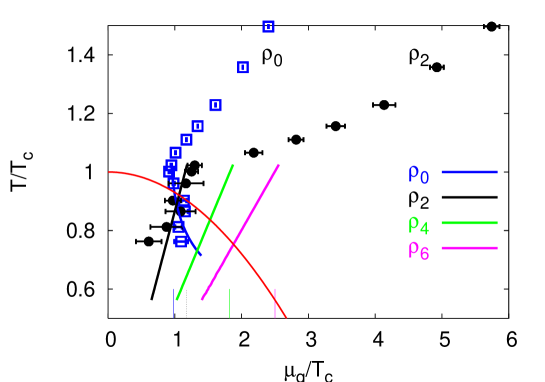
Fig. 7: Comparison between radii of convergence from the lattice Allton et al. (2003) (points) and HRGM (lines). There is an excellent agreement with the existing lattice results. The $T_{c}$-curvature has been calculated by using lattice results with two flavors (Fig. 3). The short vertical lines give the values of corresponding radii at $T_{c}$.

As we have seen, for a reliable comparison with the current lattice simulations, we have to apply truncations in the thermodynamic expressions in HRGM. Our objective here is to check the efficiency of truncated series in locating the phase diagram. The radius of convergence reflects the singularity near $T_{c}$. It approaches unity near $T_{c}$. The energy density normalized to $T^{4}$ can be expressed as a trigonometric function depending on the ratio $\mu/T$ Redlich et al. (2004) (Sec. III). We use the property that the energy density is an even function in $\mu_{B}/T$ and therefore write

$$\frac{\epsilon(T,\mu_{B})}{T^{4}} = \epsilon_{m}(T)+\epsilon_{b}(T)\cosh\left(\frac{\mu_{B}}{T}\right)$$ (29)

$$\approx \epsilon_{b}(T)\left[c_{2}\left(\frac{\mu_{q}}{T}\right)^{2}+c_{4}\left(\frac{\mu_{q}}{T}\right)^{4}\cdots\right],$$

where $c_{n}=(T_{c}/T)^{n}\;3^{n}/n!$ and $n$ is an even positive integer. The radius of convergence of Taylor expansion of the partition function, Eq. (15) is to be estimated by the ratios of subsequent expantion coefficients,

$$\rho = \lim_{n\rightarrow\infty}\left|\frac{c_{n}}{c_{n+2}}\right|^{1/2}.$$ (30)

Since the expansion is an even series of $\mu_{B}/T$, the square root is expected to arise. In order to calculate the zero order radius, we recall the results at $\mu=0$ (not included in Eq. (29)).

$$\rho_{o}=\left(\frac{c_{0}}{c_{2}}\right)^{1/2}=\frac{T}{T_{c}}\left[\frac{2}{9}\left(\frac{\epsilon_{m}(T)}{\epsilon_{b}(T,\mu_{q}=0)}+1\right)\right]^{1/2}.$$ (31)

It is clear that $\rho_{0}$, in constast to the other radii, is $T$-dependent In Fig. 7, we find that close to $T_{c}$, $\rho_{0}=0.982$, $\rho_{2}=1.18$, $\rho_{4}=1.82$ and $\rho_{6}=2.5$. These values are shown as short vertical lines. The results agree very well with the available lattice results Allton et al. (2003); as $\rho_{0}\rightarrow 1$. The radius of convergence approximately gives the lower bound for the critical endpoint ($\mu_{q}\geq T_{c}$). Obviously this value is higher than the recent lattice results Ejiri et al. (2004); Fodor and Katz (2004). In principle, one expects that due to the absence of critical behavior in HRGM, the Taylor expansion, Eq. (29), has an infinite convergence radius for all temperatures. At $T_{c}$ and for the convergence radius $\rho=1$, one expects that the hadron degrees of freedom are indistinguishable from the degrees of freedom in QGP. On the other hand, the radii $\rho$ from lattice simulations are bounded from above by the location of phase transition. Therefore, it is expected that the radii in Eq. (30) stay close to unity near $T_{c}$. In fact, this is the case for our low-order coefficients. The agreement between our results and the lattice ones is convincing. There are no published lattice results on the $6^{th}$-order radius of divergence. Nevertheless, according to our expansion coefficients, we expect that $\rho$ are steadily changing.

VII Conclusions

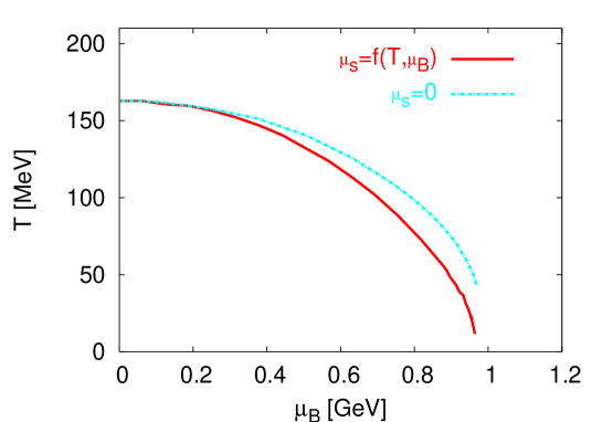
Fig. 8: Summary of our results on the QCD phase transition. In calculating both curves, we use all hadron resonances and suppose that the isospin chemical potential is vanishing. To obtain the top curve, we assigned $\mu_{s}$ to zero. $\mu_{s}$ is calculated in dependence on $T$ and $\mu_{B}$. The results are given by the bottom curve. We note that both curves will cross the abscissa at the point of normal nuclear density.

We used HRGM to draw up $T_{c}-\mu_{B}$ diagram. The transition temperature $T_{c}$ from hadronic matter to QGP has been determined according to a condition of constant energy density. Its value is taken from lattice QCD simulations at zero chemical potential and assumed to remain constant along the entire $\mu_{B}$-axis. We checked the influence of $s$ quark chemical potential $\mu_{s}$ on $T_{c}$. For including $\mu_{s}$, we applied two models. In the first one, we explicitly calculated $\mu_{s}$ in dependence on $T$ and $\mu_{B}$ under the condition that the net strangeness vanishes. In the second one, we assigned, as the case in lattice QCD simulations, zero to $\mu_{s}$ for all $T$ and $\mu_{B}$. The first case, $\mu_{s}=f(T,\mu_{B})$, is of great interest for heavy-ion collisions. Furthermore, under this consideration, we expect that the strange quantum number is entirely conserved. This is not the case in the second model. Nevertheless, with the last assignment, the current lattice results are very well reproduced. On the other hand, one can apply the second model for current and future heavy-ion collisions. At BNL-RHIC and CERN-LHC energies, for instance, $\mu_{B}$ (and consequently $\mu_{s}$) is very small. We have shown that the proper condition that guarantees vanishing strangeness in QGP is to set $\mu_{s}=\mu_{q}$. We did not check this explicitly. But it is obvious that $T_{c}(\mu_{B},\mu_{s}=0)$ quantitatively is not very much different from $T_{c}(\mu_{B},\mu_{s}(T,\mu_{B}))$ at small $\mu_{B}$.

We have taken into consideration all hadron resonances given in particle data booklet with masses up to $2\;$GeV. For a reliable comparison with lattice, we have re-scaled the resonance masses to be comparable to the quark masses used in lattice simulations. With excluding the strange resonances, we compared our results with $n_{f}=2$ lattice results. With including all resonances, we reproduced $n_{f}=2+1$ lattice results. We note that increasing $\mu_{B}$ and $\mu_{s}$ leads to monotonic decrease in $T_{c}$. The results from HRGM match very well with the lattice simulations, especially within the $\mu_{B}$-range in which the lattice calculations are most reliable ($\mu_{B}/T)\approx 3T_{c}$. The agreement turns to be excellent, when we take into consideration the truncations done in calculating the thermodynamical quantity $\epsilon$.

Besides this excellent agreement in the indirect calculation of $T_{c}$ via constant energy density, we found that the analytical expression of $T_{c}(\mu)$ up to the second order of $(\mu/T)$ greatly reproduced the curvatures calculated on lattice for different quark masses and flavor numbers.

Fig. 8 summarizes our conclusions. The QCD phase diagram is plotted for a system including light as well as strange quarks. The Taylor expansion of energy density is not truncated. The two curves represents our predictions, when it will be possible to perform lattice simulations for physical masses and without the need to truncate the Taylor expansion. As $T\rightarrow 0$, we note that both curves will cross the abscissa at almost one point. It is obvious that this point is corresponding to the normal nuclear density. The latter is related to $\mu_{B}\sim 0.979\,$GeV. The nature of the phase transition at very low temperatures does not lie within the scope of this work. However, there are many indications that the transition at $T=0$ occurs according to modification in the particle correlations. Changing the correlation leads to quantum phenomena, like quantum entropy Miller and Tawfik (2003a, b, c, 2004a); Hamieh and Tawfik (2004); Miller and Tawfik (2004b). We also note that by switching on $\mu_{s}$ an increase in $T_{c}$ is expected. At small $\mu_{B}$, the two curves are coincide.