Issues in the Extraction of $m_{s}$ and $V_{us}$ from Hadronic $\tau$ Decay Data

Abstract

Various complications encountered in the process of attempting to extract the basic Standard Model parameters, $m_{s}$ and $V_{us}$, from hadronic $\tau$ decay data are discussed.

1 Background

Hadronic $\tau$ decays into states with zero (non-zero) net strangeness provide access to the spectral functions of the correlators of the flavor $ij=ud$ ($us$) vector (V) and axial vector (A) currents, $J^{\mu}_{V/A;ij}$. Explicitly, defining $\Pi^{(J)}_{V/A}$, the $J=0,1$ parts of a given V/A correlator, and $R_{V/A;ij}$ by

$$i\,\int\,d^{4}x\,e^{iq\cdot x}\langle 0|T\left(J_{V/A}^{\mu}(x)J_{V/A}^{\nu}(0)\right)|0\rangle=$$

$$\quad\left(q^{\mu}q^{\nu}-q^{2}g^{\mu\nu}\right)\Pi^{(1)}_{V/A}(q^{2})+q^{\mu}q^{\nu}\Pi^{(0)}_{V/A}\ ,$$ (1)

$$R_{V/A;ij}\equiv{\frac{\Gamma[\tau^{-}\rightarrow\nu_{\tau}\,{\rm hadrons}_{V/A;ij}\,(\gamma)]}{\Gamma[\tau^{-}\rightarrow\nu_{\tau}e^{-}{\bar{\nu}}_{e}(\gamma)]}}\ ,$$ (2)

with ($\gamma$) denoting extra photons and/or lepton pairs, $R_{V/A;ij}$ can be expressed in terms of a weighted integral involving the corresponding spectral functions, $\rho^{(J)}_{V/A;ij}(s)$ [1, 2]:

$${\frac{R_{V/A;ij}}{\left[12\pi^{2}|V_{ij}|^{2}S_{EW}\right]}}=\int^{1}_{0}\,dy_{\tau}\,\left(1-y_{\tau}\right)^{2}$$

$$\qquad\left[\left(1+2y_{\tau}\right)\rho_{V/A;ij}^{(0+1)}(s)-2y_{\tau}\rho_{V/A;ij}^{(0)}(s)\right]$$

$$\qquad\equiv\int_{0}^{m_{\tau}^{2}}ds\,{\frac{dR_{V/A;ij}(s)}{ds}}\ ,$$ (3)

where $y_{\tau}=s/m_{\tau}^{2}$, $V_{ij}$ is the flavor $ij$ CKM matrix element, and $S_{EW}$ is an electroweak correction. The experimental decay distribution, $dR_{V/A;ij}(s)/ds$, thus yields the linear combination $w_{T}(y_{\tau})\rho_{V/A;ij}^{(0+1)}(s)+w_{L}(y_{\tau})\rho_{V/A;ij}^{(0)}(s)$, where $w_{T}(y)\equiv(1-y)^{2}(1+2y)$, $w_{L}(y)\equiv-2y(1-y)^{2}$. The $(J)=(0)$ part of Eq. (3), and of analogous OPE expressions and/or expressions involving different weights, will be called “longitudinal” in what follows.

The combinations, $\rho_{V/A;ij}^{(0+1)}(s)\equiv\rho_{V/A;ij}^{(0)}(s)+\rho_{V/A;ij}^{(1)}(s)$ and $s\rho^{(0)}_{V/A;ij}(s)$, in Eq.(3) correspond to correlator combinations (generically $\Pi(s)$) having no kinematic singularities and hence satisfying the general FESR relation

$$\int_{0}^{s_{0}}w(s)\,\rho(s)\,ds\,=\,-{\frac{1}{2\pi}}\oint_{|s|=s_{0}}w(s)\,\Pi(s)\,ds\ ,$$ (4)

valid for any $w(s)$ analytic in the region $|s|<M$ with $M>s_{0}$. Use of the OPE on the RHS of Eq. (4) allows one to determine OPE parameters in terms of experimental spectral distributions. Many authors have employed the “$(k,m)$ spectral weight sum rules”, for which the integrand on the LHS of Eq. (4) is $(1-y_{\tau})^{k}y_{\tau}^{m}\,dR_{V/A;ij}(s)/ds$. These sum rules are “inclusive”, in the sense that the $(k,m)$ spectral integrals, denoted $R^{(k,m)}_{V/A;ij}$, can be constructed from the experimental distribution without having to first perform a separation of the $J=0$ and $J=1$ components.

In flavor-breaking differences such as $\Pi^{(0+1)}_{V/A;ud}(s)-\Pi^{(0+1)}_{V/A;us}(s)$ or $s\,\Pi^{(0)}_{V/A;ud}(s)$-$s\,\Pi^{(0)}_{V/A;us}(s)$, the leading $D=0$ OPE terms cancel, leaving as leading contribution a $D=2$ term, essentially proportional to $m_{s}^{2}$. Appropriately-weighted FESR’s involving such differences thus, in principle, allow one to determine $m_{s}$. Flavor-breaking spectral combinations of the $(k,m)$ spectral weight type are constructed by forming

$$\Delta R^{(k,m)}_{V/A;ij}\equiv{\frac{R^{(k,m)}_{V/A;ud}}{V_{ud}^{2}}}-{\frac{R^{(k,m)}_{V/A;us}}{V_{us}^{2}}}\ .$$ (5)

A number of determinations of $m_{s}$ using flavor-breaking sum rules have appeared in the literature [4, 5, 6, 7]. We discuss some non-trivial complications, not all of which have been effectively tamed in the majority of these analyses, below.

Recently it has been realized that $\tau$-decay-based, flavor-breaking sum rules also provide a novel method for extracting $V_{us}$ [6], one whose systematics are completely independent of those associated with alternate determinations based either on combining lattice results for $f_{\pi}/f_{K}$ with $\pi_{\ell 2}$ and $K_{\ell 2}$ data [9] or on $K_{\ell 3}$ [8].

The $\tau$-decay-based determination is competitive for the following reason. The difference of rescaled $ud$ and $us$ spectral integrals corresponds to an integrated correlator difference with exactly cancelling $D=0$ OPE contributions only if the correct $V_{us}$ is used to rescale the experimental $us$ data. An incorrect $V_{us}$ leaves a residual $D=0$ contribution. Since the $D=2$ term in the $us$ V+A OPE is very small compared to the leading $D=0$ term, even a small error in $V_{us}$ yields a sizeable $D=0$ residual. The integrated $D=0$ and $D=2$ OPE contributions scale differently with $s_{0}$, so such a $D=0$ residual can be detected by studying the $s_{0}$ dependence of the two sides of the resulting FESR. If one has external information on $m_{s}$, this can also be used as input on the OPE side in order to determine the $V_{us}$ value for which the desired $D=0$ cancellation occurs. An ideal sum rule for this purpose would be one for which the weighted $D=2$ OPE integrals were as small as possible, reducing errors associated with uncertainties in the input value of $m_{s}$, and/or possible slow convergence of the integrated $D=2$ series. For such a sum rule, the fractional uncertainty on $V_{us}$ would be essentially half that on the integrated $us$ spectral integral, a figure which could be rather small when B factory spectral data is finally available. This ideal situation is not as well realized as one might hope for most of the weights discussed to date in the literature. We discuss this point further below.

2 Complications in the Extraction of $m_{s}$ and $V_{us}$ From Hadronic $\tau$ Decay Data

Four main complications are encountered in analyzing flavor-breaking $\tau$-decay-based FESR’s: (i) the bad behavior of the integrated $D=2$ longitudinal OPE series; (ii) the convergence (order by order in $\alpha_{s}$) of the integrated $(J)=(0+1)$ $D=2$ OPE series; (iii) the role of possible $D>6$ OPE contributions and (iv) strong $ud$-$us$ spectral integral cancellations for many of the weights employed in the literature (leading to significant fractional errors on the resulting difference, and hence also in the extracted values of $m_{s}$).

2.1 The Integrated $D=2$ Longitudinal OPE Contribution

It has been known for some time that the convergence of the integrated $D=2$ longitudinal OPE series relevant to the determination of $m_{s}$ is very poor [10]. In “contour improved perturbation theory” (CIPT), e.g., even at the highest possible scale, $s_{0}=m_{\tau}^{2}$, the integrated $(0,0)$ series behaves as $1+0.78+0.78+0.90+\cdots$. The non-convergence is even worse in fixed order perturbation theory, and/or for $s_{0}<m_{\tau}^{2}$. One obvious solution is to restrict one’s attention to the better-behaved $(J)=(0+1)$ sum rules, where the problem does not arise. This, however, requires a separation of the $J=0,1$ components of the experimental spectral distribution, which is not feasible experimentally at present. Many analyses have, therefore, employed “inclusive” ($(J)=(0)$ plus $(J)=(0+1)$) sum rules and attempted to assign conservative errors to the $O(\alpha_{s}^{3})$-truncated, badly-converged integrated $D=2$ longitudinal OPE sum. This procedure turns out to violate inequalities among longitudinal contributions to the flavor-breaking $(k,0)$ spectral weight sum rules which folow from the positivity of $\rho^{(0)}_{V;us}$ and/or $\rho^{(0)}_{A;us}$ [11]. We elaborate on this point in the next paragraph.

While the $\pi$ and $K$ pole contributions to the longitudinal spectral functions are well known experimentally, the “continuum” contributions (beginning at $s_{th}^{V}=(m_{K}+m_{\pi})^{2}$ and $s_{th}^{A}=(m_{K}+2m_{\pi})^{2}$ in the $us$ V and A channels, respectively) are not. For the flavor $ud$ correlators, these are proportional to $m_{u,d}^{2}$, and numerically negligible. The chiral suppression is of $O(m_{s}^{2})$ and hence much less strong for the $us$ V, A correlators. The basic FESR relation, combined with the known pole term values, ensures that any prescription for handling the weighted longitudinal $us$ $D=2$ OPE series translates into a statement about the correspondingly-weighted longitudinal continuum spectral integral. Denote this contribution by $\left[\Delta^{(k,m)}\right]^{c}_{L}$ for the $(k,m)$ spectral weight case. Then, since $0<(1-y_{\tau})<0.87$ for $s_{th}^{V}<s<m_{\tau}^{2}$, spectral positivity ensures that the $\left[\Delta^{(k,0)}\right]^{c}_{L}$ must (i) be a decreasing function of $k$ and (ii) satisfy the rigorous inequalities

$$\left[\Delta^{(k+1,0)}\right]_{L}^{c}<0.87\left[\Delta^{(k,0)}\right]_{L}^{c}\ .$$ (6)

For kinematic reasons, one expects the $K(1460)$ and $K_{0}^{*}(1430)$ resonances to dominate $\left[\Delta^{(k,0)}\right]^{c}_{L}$. Neglecting other contributions, the even stronger constraints $\left[\Delta^{(1,0)}\right]_{L}^{c}\simeq 0.44\left[\Delta^{(0,0)}\right]_{L}^{c}$ and $\left[\Delta^{(2,0)}\right]_{L}^{c}\simeq 0.22\left[\Delta^{(0,0)}\right]_{L}^{c}$ are obtained. The $k=0,1,2$ $\left[\Delta^{(k,0)}\right]^{c}_{L}$ implied by the $O(\alpha_{s}^{3})$ $D=2$ OPE truncation prescription (employing a $k$-independent $m_{s}$) are, in contrast, in the ratios $1:1.16:1.42$, badly violating even the weaker constraint, Eq. (6). Since the experimental spectral distribution necessarily respects spectral positivity, independent fits for $m_{s}$ using different $(k,0)$ FESR’s will, unavoidably, produce central values having an unphysical decrease with $k$. Such a decrease is seen in all inclusive $(k,0)$ analyses. A large portion of the observed instability-with-$k$ can be attributed to the violation of spectral positivity [12]. Much improved stability is obtained for the longitudinally-subtracted $(J)=(0+1)$ version of the $(k,0)$ analysis [7].

The absence of an experimental spin separation means that, to avoid the above problems, and work with the better-behaved $(J)=(0+1)$ sum rules, one needs theoretical input for the unknown (continuum) part of the longitudinal spectral distribution. The flavor $us$ A part can be obtained from the results of Ref. [13] (which determines the excited $K$ decay constants from a sum rule analysis of the flavor $us$ pseudoscalar correlator); the flavor $us$ V part, similarly, from a detailed study of the related flavor $us$ scalar correlator [14]. Details may be found in the original references . It turns out that, even if one assigns very conservative errors ($\sim 50\%$) to these determinations, the impact on the uncertainties in the resulting longitudinally-subtracted $(J)=(0+1)$ sum rules is small. The reason is easily understood.

To simplify discussion, consider the narrow width approximation (NWA) for the $K(1460)$ and $K_{0}^{*}(1430)$. The corresponding decay constants, $f$, vanish in the $SU(3)$ chiral limit and hence receive a chiral suppression (proportional to $m_{s}$) for physical $m_{s}$. The corresponding longitudinal spectral contributions ($\propto f^{2}$) are thus doubly chirally suppressed relative to the $\pi$ and $K$ pole terms. In the NWA, taking the $(0,0)$ spectral weight case to be specific, the integrated longitudinal contribution of a scalar or pseudoscalar state of mass $M$ is proportional to

$${\frac{2M^{2}}{m_{\tau}^{2}}}\left(1-{\frac{M^{2}}{m_{\tau}^{2}}}\right)^{2}\,f^{2}\ .$$ (7)

The kinematic factor, ${\frac{2M^{2}}{m_{\tau}^{2}}}\left(1-{\frac{M^{2}}{m_{\tau}^{2}}}\right)^{2}$, is $0.13$ for the $K$ and $\sim 0.15$ for the $K_{0}^{*}(1430)$ and $K(1460)$. Thus, the relative size of the integrated longitudinal continuum and $K$ pole contributions is determined almost entirely by the square of the ratio of the corresponding decay constants, and is doubly chirally suppressed. Since the $K$ pole contribution is very accurately known, even rather large errors on the continuum contribution will correspond to small errors on the full (pole plus continuum) longitudinal spectral integral. The subtraction needed to go from the inclusive experimental $(0,0)$ spectral integral to the analogous $(J)=(0+1)$ component thereof can thus be performed with good accuracy. Extra factors of $\left(1-M^{2}/m_{\tau}^{2}\right)$, present for the higher $(k,0)$ sum rules, will further suppress continuum contributions relative to the leading $K$ pole term, making the longitudinal subtraction even more reliable.

In summary, (i) the conclusion that only non-inclusive, $(J)=(0+1)$ flavor-breaking FESR’s should be employed in future seems unavoidable, in view of the severity of the problems with the corresponding inclusive FESR’s; (ii) the longitudinal subtraction needed for a determination of the spectral integrals of the $(J)=(0+1)$ sum rules is dominated by the well-known $K$ pole term, and can be performed with good accuracy, with the results of Refs. [13, 14] to be used for the small flavor $us$ continuum contributions; (iii) having accepted the necessity of performing a longitudinal subtraction, one of the major arguments in favor of the use of the $(k,m)$ spectral weights (the possibility of avoiding a spin separation of the experimental spectral data) is no longer operative, and one is free to explore alternate weight choices which may improve the accuracy with which the OPE and/or spectral integral sides of the resulting flavor-breaking $(J)=(0+1)$ sum rules can be evaluated.

We will return to the latter point below.

2.2 Convergence of the Integrated $(0+1)$ OPE Series

The necessity of a longitudinal subtraction means that one must focus on sum rules for the flavor-breaking $(J)=(0+1)$ correlator. Experimental and theoretical uncertainties are reduced by working with the difference of the V+A sums for the flavor $ud$ and $us$ cases. Two points, related to the question of the convergence of the integrated OPE series, require discussion: the behavior of the integrated $D=2$ series, and the treatment of contributions with $D>6$.

2.2.1 The $D=2$ OPE Series

In the $\overline{MS}$ scheme, the $D=2$ term in the OPE of the $(J)=(0+1)$ V+A $us$ correlator is proportional to $\left[m_{s}(Q^{2})\right]^{2}/Q^{2}$ times the series [15]

$$1+{\frac{7}{3}}a+19.58a^{2}+202.3a^{3}+(2200\pm 200)a^{4}+\cdots$$ (8)

where $a=\alpha_{s}(Q^{2})/\pi$ and the $O(a^{4})$ coefficient is the PMS estimate based on the $O(a^{3})$ result reported by Chetyrkin at this meeting [15]. Since $a(m_{\tau}^{2})\simeq 0.10$, the convergence of the last few terms of the series is actually very slow at the spacelike point on the circle $|s|=s_{0}$, even at the largest scale, $s_{0}=m_{\tau}^{2}$, allowed by kinematics. As one moves along the circle toward the timelike point, however, the logarithmic running of $\alpha_{s}$ causes $|\alpha_{s}\left(Q^{2}\right)|$ to decrease, improving the convergence of the correlator series. Different choices of FESR weight, which emphasize different regions of the circle, can thus lead to integrated $D=2$ series with significantly different convergence behaviors. Within the $(k,0)$ spectral weight family, e.g., one expects increasing $k$ to produce slower convergence, since the additional factors of $(1-s/s_{0})$ weight more and more heavily contributions from the part of the circle near the spacelike point, where convergence is slowest. Cancellations on the contour can also play a role in determining the convergence of the integrated series.

The convergence behavior of the integrated $ud$-$us$ V+A, $(J)=(0+1)$ $D=2$ OPE series for the $(k,0)$ spectral weights is illustrated in Table 1. The contributions have been evaluated using CIPT, for $s_{0}=m_{\tau}^{2}$. The results are normalized to the leading ($O(a^{0})$) term. We have included an $O(a^{4})$ contribution generated using the PMS estimate for the $O(a^{4})$ correlator coefficient. The pattern of convergence is typically somewhat worse if one works with the Adler function, rather than the correlator itself (see Chetyrkin’s talk at this meeting for more on this point). The convergence also deteriorates significantly as $s_{0}$ decreases. Note that the convergence of the $(0,0)$ series is not good, despite the impression an $O(a^{2})$ truncation might give. The $O(a^{2})$ contribution happens to be small because of cancellations among contributions from different parts of the OPE contour; this cancellation, however, is “accidental”, in the sense that it does not persist for higher order contributions. Similar accidental cancellations occur for the other $(k,0)$ cases, though at orders which increase with $k$; as a result, only a hint of this behavior shows up in the table for $k=2,3,4$.

Table 1: Convergence of integrated $(0+1)$ $D=2$ OPE series for the $(k,0)$, $k=0,\cdots,4$ spectral weights

Weight:	(0,0)	(1,0)	(2,0)	(3,0)	(4,0)
$O(a^{0})$	1	1	1	1	1
$O(a^{1})$	.14	.21	.26	.30	.33
$O(a^{2})$	-.01	.10	.19	.27	.34
$O(a^{3})$	-.18	-.04	.09	.21	.34
$O(a^{4})$	-.38	-.23	-.08	.09	.28

The disappointing convergence of the $D=2$ series for the $(k,0)$ spectral weights is not a general feature of flavor-breaking V+A, $(J)=(0+1)$ FESR’s. In fact, by studying the behavior of the correlator in the complex plane, it is possible to construct weights which emphasize precisely those regions of the contour where the OPE is not only reliable but displays improved $D=2$ convergence [5]. Three weights of this type were discussed in Ref. [5]. For these weights, in contrast to the $(k,0)$ spectral weights, the suppression of higher order integrated $D=2$ contributions results from a dominance by the region of improved correlator convergence, and not from an order-dependent accidental cancellation along the contour. For this reason, the improved convergence persists even to much higher orders [5]. Employing the information reported by Chetyrkin for the values of the $O(a^{3},a^{4})$ coefficients [15], the $s_{0}=m_{\tau}^{2}$ contour-improved integrated $D=2$ series for these weights behave as

$$1+.26+.21+.17+.11\ ({\rm for\ }w_{20})$$

$$1+.23+.17+.11+.05\ ({\rm for\ }w_{10}),\ {\rm and}$$

$$1+.25+.19+.15+.10\ ({\rm for\ }\hat{w}_{10})\ .$$ (9)

In summary, (i) the convergence of the integrated $(J)=(0+1)$, V+A $ud$-$us$ $D=2$ series for the $(k,0)$ spectral weights is problematic (this is particularly true of the $(0,0)$ case, although this fact does not become evident until one goes beyond $O(a^{2})$); (ii) alternate weight choices exist with improved $D=2$ convergence.

2.2.2 $D>6$ OPE Contributions

The OPE series for the $ud$-$us$ $(J)=(0+1)$, V+A correlator difference is known up to terms of dimension $D=6$. The $D=4$ contribution is well determined phenomenologically, and the $D=6$ term can be estimated using the vacuum saturation approximation (VSA). It turns out that $D=6$ contributions to those FESR’s studied in the literature are small, even if one assigns a factor $5-10$ error to the VSA result. $D>6$ contributions are not known; nor are phenomenological values available for a full set of $D>6$ condensates. In existing flavor-breaking $\tau$-decay-based analyses, $D>6$ contributions have been assumed to be safely negligible at the scales employed, usually without explicit tests of this assumption. We point out below how such tests may be carried out, and explain why, for certain of the $(k,0)$ spectral weights, results obtained in the absence of such tests should be viewed with caution.

Consider a polynomial weight, $w(y)=\sum_{k=0}^{N}b_{k}y^{k}$, written in terms of the natural variable $y=s/s_{0}$. The “pinching” condition (necessary for the reliability of the OPE at intermediate scales) is $w(1)=0$. A term $C_{D}/Q^{D}$ in the OPE yields a contribution to the $w(y)$-weighted OPE integral proportional to $b_{\kappa_{D}}\,C_{D}/s_{0}^{\kappa_{D}}$, with $\kappa_{D}=(D-2)/2$. The fact that integrated OPE contributions with different $D$ scale differently with $s_{0}$ allows one to test the assumption that higher $D$ terms are safely negligible by studying the $s_{0}$ dependence of any sum rule output.

As an example, the $(4,0)$ weight, having degree 7, in principle produces integrated OPE contributions up to $D=16$. If a nominal determination of, e.g., $m_{s}$ using the $(4,0)$ FESR has incorrectly assumed that $D>6$ terms can be neglected, this will show up as a variation of $m_{s}$ with $s_{0}$. This variation results from the fact that the integrated $D=2$ term, from which $m_{s}$ is determined, scales as a constant (up to logarithmic corrections), but has been forced to absorb the effect of contributions with $D>6$, which scale like $1/s_{0}^{N}$, with $N\geq 3$. It is crucial to perform this $s_{0}$-stability test, especially for polynomials $w(y)$ having coefficients, $b_{k}$, with $k\geq 3$, which are large.

For the $(k,0)$ spectral weights, the relevant polynomial coefficients grow with $k$; hence so does the danger of neglecting $D>6$ contributions. The explicit forms of the $(J)=(0+1)$ $(k,0)$ weights, $w^{(k,0)}(y)=(1-y)^{k}\,w_{T}(y)$, are

$${w}^{(0,0)}(y) = 1-3y^{2}+2y^{3}$$

$${w}^{(1,0)}(y) = 1-y-3y^{2}+5y^{3}-2y^{4}$$

$${w}^{(2,0)}(y) = 1-2y-2y^{2}+8y^{3}-7y^{4}+2y^{5}$$

$${w}^{(3,0)}(y) = 1-3y+10y^{3}-15y^{4}+9y^{5}-2y^{6}$$

$${w}^{(4,0)}(y) = 1-4y+3y^{2}+10y^{3}-25y^{4}+24y^{5}$$ (10)

$$\ \ \ \ \ \-11y^{6}+2y^{7}\ .$$

The $O(y^{4})$ and $O(y^{5})$ coefficients in $w^{(4,0)}(y)$, e.g., which govern the integrated $D=10$ and $12$ OPE contributions to the $(4,0)$ FESR, are more than an order of magnitude larger than the $O(y^{3})$ coefficient in $w^{(0,0)}(y)$, which governs the integrated $D=8$ contribution to the $(0,0)$ FESR. Neglect of $D>6$ contributions is thus far safer in the $(0,0)$ than in the $(4,0)$ case.

The alternate weights of Ref. [5] were constructed to have coefficients $b_{k}$, $k\geq 3$, as small as possible, given other constraints. With the $O(y^{0})$ terms normalized to $1$, as for the $(k,0)$ weights, the largest of these $b_{k}$’s is 1.206 for $\hat{w}_{10}$, $2$ for $w_{10}$ and $2.087$ for $w_{20}$. Neglect of $D>6$ contributions is thus much safer than it is for the higher $(k,0)$ spectral weights, though one should, of course, still perform $s_{0}$-stability checks in all cases.

2.3 Cancellations in the $ud$-$us$ Spectral Difference

One might naively expect the cancellation on the spectral integral side of a flavor-breaking $ud$-$us$ FESR to be at the $\sim 20-30\%$ level, the typical scale of $SU(3)_{F}$ breaking. With present $ud$-$us$ spectral integral errors dominated by the $us$ contribution, and these errors being at the $\sim 3\%$ level for $s_{0}=m_{\tau}^{2}$, $\sim 10\%$ errors would then be expected for the $ud$-$us$ difference. Unfortunately, this naive estimate is not borne out: for weights considered in the literature, the cancellation is much stronger, leading to much larger fractional errors on the $ud$-$us$ difference. Since the level of cancellation depends on the weight, $w(y)$, the accuracy of the extraction of a quantity such as $m_{s}$, from a given set of experimental data, can be improved by a judicious choice of weight(s).

Table 2 shows the ratio of $ud$-$us$ to $ud$ spectral integrals for $s_{0}=m_{\tau}^{2}$, for $(J)=(0+1)$, V+A FESR’s based on (i) the $(k,0)$ spectral weights, and (ii) the weights, $w_{10}$, $\hat{w}_{10}$, and $w_{20}$ of Ref. [5]. CKMU labels results corresponding to the central PDG04 unitarity-constrained fit values, $V_{ud}=0.9745$, $V_{us}=0.2240$, CKMN results corresponding to the central PDG04 independent fit values, $V_{ud}=0.9738$, $V_{us}=0.2200$.

Table 2: $ud$-$us$ spectral cancellation level for various weights and for two choices of the input CKM values, $V_{ud}$ and $V_{us}$

Weight	CKMN	CKMU
$(0,0)$	0.6$\%$	4.0$\%$
$(1,0)$	4.5$\%$	7.8$\%$
$(2,0)$	8.3$\%$	11.4$\%$
$(3,0)$	11.9$\%$	14.9$\%$
$(4,0)$	15.6$\%$	18.5$\%$
$w_{10}$	3.7$\%$	7.0$\%$
$\hat{w}_{10}$	4.4$\%$	7.7$\%$
$w_{20}$	7.5$\%$	10.6$\%$

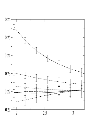
Figure 1: Stability of various FESR analyses for $V_{us}$. The vertical axis shows $V_{us}$, the horizontal axis $s_{0}$ in GeV². The curves, from top to bottom on the LHS of the figure, correspond to the weights $w^{(4,0)}$, $w^{(3,0)}$, $w_{20}$, $w^{(2,0)}$ (dashed line), $w_{10}$ (solid line) and $w^{(0,0)}$.

The results show a high level of sensitivity to CKM input for those weights having the strongest cancellation. The strong cancellation also leads to large fractional errors for the integrated $ud$-$us$ differences. This effect is responsible, e.g., for the large errors quoted on $(0,0)$ spectral weight FESR determinations of $m_{s}$ in the literature. Large shifts in the central values of $m_{s}$ caused by apparently rather small changes in the total strange branching fraction value are also the result of this high level of cancellation. (Another example of this effect will be seen in the next section.) The cancellation is at a much more acceptable level for the $(3,0)$ and $(4,0)$ weights. Unfortunately, as we have seen above, these weights have rather slow $D=2$ convergence, as well as large coefficients which make neglect of $D>6$ contributions more problematic. More accurate $us$ data, especially in the region above $\sim 1\ {\rm GeV}^{2}$, might allow alternate weights to be constructed which deal with this problem more effectively, without producing a deterioration in the $ud$-$us$ error situation.

In view of the above-noted “close cancellations”, it is desirable to reduce, where feasible, the error on any particular $ud$-$us$ spectral integral. Evaluating the $\pi$ and $K$ pole term contributions using the more accurate $f_{\pi}V_{ud}$ and $f_{K}V_{us}$ $\pi_{\ell 2}$ and $K_{\ell 2}$ determinations is helpful in this regard. While one should obviously check that $\tau$ decay determinations of the $\tau\rightarrow\pi\nu_{\tau}$ and $\tau\rightarrow K\nu_{\tau}$ BR’s are compatible with Standard Model (SM) expectations based on $\pi_{\ell 2}$ and $K_{\ell 2}$ data, attempts to extract $m_{s}$ and/or $V_{us}$ from $\tau$ decay data are predicated on the assumption that beyond-the-SM effects may be neglected in $\tau$ decay; there is, thus, no compelling reason to use the larger-error $\tau$-decay-based pole term values in such analyses.

3 An Illustrative Example

We illustrate some features of the above discussion by considering a determination of $V_{us}$ analogous to that reported in Ref. [7]. A value $m_{s}(2\ {\rm GeV}^{2})=95\pm 20$ MeV, representing an average (with conservative errors) from non-$\tau$-decay based determinations is used on the OPE side of the various FESR’s. The corresponding spectral integrals are based on the recently-reported OPAL update of the $us$ spectral database [19], with the following caveats. At present, neither the numerical values of the OPAL $us$ spectral distribution nor the corresponding covariance matrix have been made publicly available. OPAL has reported spectral integrals, with fully correlated errors, only for the $(k,0)$ spectral weights, and, for these, only at $s_{0}=m_{\tau}^{2}$. To work out spectral integrals for either non-spectral weights, or for spectral weights, but at $s_{0}<m_{\tau}^{2}$, we follow the strategy used previously by ALEPH (see the two papers by S. Chen et al. in Ref. [4]). Explicitly, we start with the 1999 ALEPH $us$ spectral distribution [20] and rescale that part of the spectral distribution associated with each exclusive mode by the corresponding ratio of current to ALEPH 1999 branching fractions. To guide the eye we include “experimental” errors generated using the publicly-available ALEPH covariance matrix. We have also employed $\pi_{\ell 2}$ and $K_{\ell 2}$ results in evaluating the $\pi$ and $K$ pole term contributions. The results of this exercise for a selection of the weights discussed above, as a function of $s_{0}$, are shown in Fig. 1. To avoid (further) cluttering the figure, OPE errors have not been included.

The figure shows considerable instability for the $(0,0)$, $(3,0)$ and $(4,0)$ spectral weights. Good stability is observed for $w_{10}$, $w_{20}$ and the $(2,0)$ spectral weight. The instability of the $(0,0)$ determination is almost certainly a consequence of the poor convergence behavior of the integrated $D=2$ OPE series. The $s_{0}$ dependence, together with the comparison of the results for the range of different weights shown, gives one confidence in an extracted value of $V_{us}$ represented by the convergence of the four lowest weight cases as $s_{0}\rightarrow m_{\tau}^{2}$ in the figure, $V_{us}\simeq 0.2209$. More detailed results, with realistic experimental and OPE errors will be reported elsewhere.

We conclude with a further illustration of the sensitivities of output parameters to small changes in experimental data, resulting from strong cancellations in the $ud$-$us$ spectral integral differences. The above result for $V_{us}$ employed the world average, $B=0.0033$, for the $K^{-}\pi^{+}\pi^{-}$ branching fraction. If one instead shifts to the average, $B=0.0040$, of the OPAL and CLEO determinations, which are in good agreement, and not in good agreement with ALEPH, the central value of $V_{us}$, e.g., from the good-stability $w_{10}$ extraction, changes from $0.2209$ to $0.2232$.

Further details of the $V_{us}$ analysis, and of the related $m_{s}$ analysis, will be reported elsewhere.

References

- [1] E. Braaten, Phys. Rev. Lett. 60 (1988) 1606; S. Narison and A. Pich, Phys. Lett. B211 (1988) 183 and Phys. Lett. B304 (1993) 359; E. Braaten, Phys. Rev. D39 (1989) 1458; E. Braaten, S. Narison, A. Pich, Nucl. Phys. B373, 581 (1992).
- [2] A review and extensive list of earlier references may be found in A. Pich, Nucl. Phys. Proc. Suppl. 39BC (1995) 326.
- [3] K. Maltman, Phys. Lett. B440 (1998) 367.
- [4] A. Pich, J. Prades, JHEP 06 (1998) 013; K.G. Chetyrkin, J.H. Kuhn, A.A. Pivovarov, Nucl.Phys. B533 (1998) 473; A. Pich, J. Prades, JHEP 9910 (1999) 004; J.G. Körner, F. Krajewski, A.A. Pivovarov, Eur. Phys. J. C14 (2000) 123 and Eur. Phys. J. C20 (2001) 259; S. Chen, M. Davier, E. Gamiz, A. Höcker, A. Pich, J. Prades, Eur. Phys. J. C22 (2001) 31, Eur. Phys. J. C22 (2001) 31.
- [5] J. Kambor, K. Maltman, Phys. Rev. D62 (2000) 093023.
- [6] E. Gamiz et al., JHEP 0301 (2003) 060.
- [7] E. Gamiz et al., hep-ph/0408044.
- [8] H. Leutwyler, M. Roos, Z. Phys. C25 (1984) 91; V. Cirigliano, H. Neufeld, H. Pichl, E. Phys. J. C35 (2004) 53.
- [9] W. J. Marciano, hep-ph/0402299; C. Aubin et al. (MILC), hep-lat/0407028.
- [10] K. Maltman, Phys. Rev. D58 (1998) 093015; K.G. Chetyrkin, A. Kwiatkowski, Z. Phys. C59 (1993) 525; hep-ph/9805232.
- [11] J. Kambor, K. Maltman, Phys. Rev. D64 (2001) 093014.
- [12] K. Maltman, hep-ph/0209091.
- [13] K. Maltman, J. Kambor, Phys. Lett. B517 (2001) 332; Phys. Rev. D65 (2001) 074013.
- [14] M. Jamin, J.A. Oller and A. Pich, Nucl. Phys. B587 (2000) 331; Nucl. Phys. B622 (2002) 279; Eur. Phys. J. C24 (2002) 237.
- [15] K. Chetyrkin, presentation at Tau’04.
- [16] P.A. Baikov, K.G. Chetyrkin, J.H. Kuhn, Phys. Rev. D67 (2003) 074026.
- [17] S. Narison, Phys. Lett. B361 (1995) 121; K. Maltman and C.E. Wolfe, Phys. Rev. D59 (1999) 096003.
- [18] V. Cirigliano et al., Phys. Lett. B522 (2001) 245 and Phys. Lett. B555 (2003) 71; V. Cirigliano, E. Golowich, K. Maltman, Phys. Rev. D68 (2003) 054013.
- [19] G. Abbiendi et al., Eur. Phys. J. C34 (2004) 437.
- [20] R. Barate et al., Eur. Phys. J. C11 (1999) 511.