DESY 04-237 December 2004 Dual Models of Gauge Unification
in Various Dimensions

Abstract

We construct a compactification of the heterotic string on an orbifold $T^{6}/\mathbbm{Z}_{6}$ leading to the standard model spectrum plus vector–like matter. The standard model gauge group is obtained as an intersection of three $\mathrm{SO}(10)$ subgroups of $\mathrm{E}_{8}$. Three families of $\mathrm{SO}(10)$ ${\bf 16}$-plets are localized at three equivalent fixed points. Gauge coupling unification favours existence of an intermediate GUT which can have any dimension between five and ten. Various GUT gauge groups occur. For example, in six dimensions one can have $\mathrm{E}_{6}\times\mathrm{SU}(3)$, $\mathrm{SU}(4)\times\mathrm{SU}(4)\times\mathrm{U}(1)^{2}$ or $\mathrm{SO}(8)\times\mathrm{SO}(8)$, depending on which of the compact dimensions are large. The different higher–dimensional GUTs are ‘dual’ to each other. They represent different points in moduli space, with the same massless spectrum and ultraviolet completion.

1 Embedding the standard model in $\boldsymbol{\mathrm{E}_{8}}$

The symmetries and the particle content of the standard model point towards grand unified theories (GUTs) as the next step in the unification of all forces. Left- and right-handed quarks and leptons can be grouped in three $\mathrm{SU}(5)$ multiplets [1], $\boldsymbol{10}=(q_{\mathrm{L}},u_{\mathrm{R}}^{c},e_{\mathrm{R}}^{c})$, $\boldsymbol{\overline{5}}=(d_{\mathrm{R}}^{c},\ell_{\mathrm{L}})$ and $\boldsymbol{1}=\nu_{\mathrm{R}}^{c}$. Here we have added right-handed neutrinos which are suggested by the evidence for neutrino masses. All quarks and leptons of one generation can be unified in a single multiplet of the GUT group $\mathrm{SO}(10)$ [2],

$$\boldsymbol{16}=\boldsymbol{10}+\boldsymbol{\overline{5}}+\boldsymbol{1}\;.$$ (1)

The group $\mathrm{SO}(10)$ contains as subgroups the Pati-Salam group [3], $G_{\rm PS}=\mathrm{SU}(4)\times\mathrm{SU}(2)\times\mathrm{SU}(2)$, the Georgi-Glashow group $\mathrm{SU}(5)$, $G_{\rm GG}=\mathrm{SU}(5)\times\mathrm{U}(1)$, and the ‘flipped’ $\mathrm{SU}(5)$ group, $G_{\rm fl}=\mathrm{SU}(5)^{\prime}\times\mathrm{U}(1)^{\prime}$ [4], where the right-handed up- and down-quarks are interchanged, yielding another viable GUT group.

It is a remarkable property of the standard model that the matter fields form complete $\mathrm{SO}(10)$ multiplets whereas the gauge and Higgs fields are ‘split multiplets’. They have to be combined with other split multiplets, not contained in the standard model, in order to obtain a complete unified theory. It is also well known [5] that exceptional groups play an exceptional role in grand unification, and the embedding

$$\mathrm{SO}(10)\subset\mathrm{E}_{6}\subset\mathrm{E}_{8}$$ (2)

appears, in particular, in compactifications of the heterotic string [6] on Calabi-Yau manifolds [7].

As we shall see, complete $\mathrm{SO}(10)$ matter multiplets together with split gauge and Higgs multiplets arise naturally in orbifold compactifications of higher-dimensional unified theories. Orbifold compactifications have first been considered in string theory [8, 9] and subsequently in effective higher-dimensional field theories [10, 11]. They provide a simple and elegant way to break GUT symmetries, while avoiding the notorious doublet-triplet splitting problem. More recently, it has been shown how orbifold GUTs can occur in orbifold string compactifications [12, 13, 14].

In the following we shall first search for a scheme of $\mathbbm{Z}_{N}$ twists which allows to break $\mathrm{E}_{8}$, a common ingredient of string models, to the standard model group. A $\mathbbm{Z}_{N}$ twist is an element of the gauge group $G$, with

$$P=\exp{(-2\pi\mathrm{i}V_{N}\cdot\boldsymbol{H})}\;,\quad P^{N}=\mathbbm{1}\;.$$ (3)

Here the generators $\boldsymbol{H}_{i}$ form the (Abelian) Cartan subalgebra of $G$, and $V_{N}$ is a real vector. The twist $P$ acts on the Cartan and step generators $\boldsymbol{E}_{\alpha}$ as follows:

$$P\,\boldsymbol{H}_{i}\,P^{-1} = \boldsymbol{H}_{i}\,$$

$$P\,\boldsymbol{E}_{\alpha}\,P^{-1} = \exp{(-2\pi\mathrm{i}V_{N}\cdot\alpha)}\,\boldsymbol{E}_{\alpha}\;,$$ (4)

where $\alpha$ is a root associated with $\boldsymbol{E}_{\alpha}$. Clearly, $P$ breaks $G$ to a subgroup containing all step generators which commute with $P$, i.e. $[P,\boldsymbol{E}_{\alpha}]=0$.

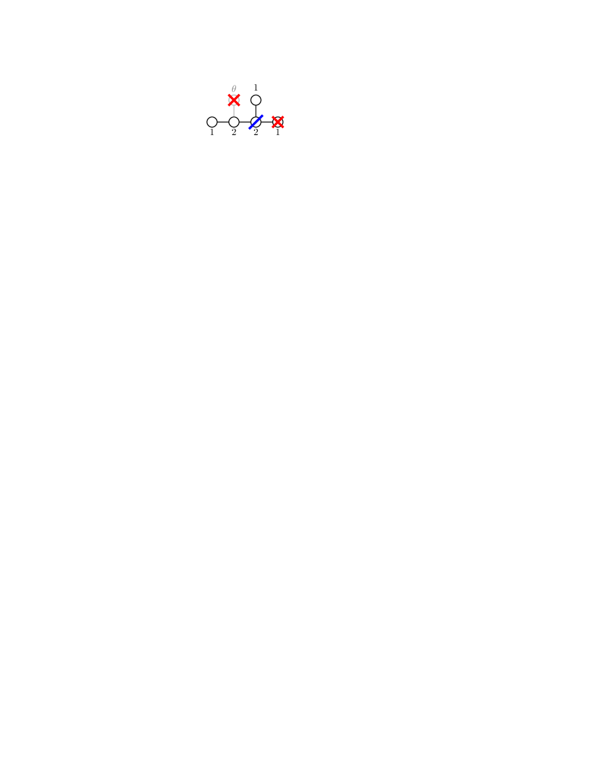
Figure 1: $\mathrm{SO}(10)$ breaking patterns by a $\mathbbm{Z}_{2}$ twist. The action of the Pati-Salam twist is indicated by crosses, while that of the Georgi-Glashow twist is indicated by a slash.

The symmetry breaking is conveniently expressed in terms of the Dynkin diagrams. This technique has been employed to classify possible symmetry breaking patterns in string models [15, 16, 17] and, more recently, in orbifold GUTs [18, 19]. Starting with the extended Dynkin diagram which contains the most negative root in addition to the simple roots, regular subgroups of a given group are obtained by crossing out some of the roots of the Dynkin diagram. In particular, the action of the $\mathbbm{Z}_{N}$ orbifold twist essentially amounts to crossing out a root with the (Coxeter) label $N$, or more generally, roots whose labels sum up to $\leq N$.

As an example, consider the breaking of $\mathrm{SO}(10)$, displayed in Fig. 1. For each simple root the Coxeter label is listed, which determines the order of the twist required for the corresponding symmetry breaking. Crossing out one of the nodes with label 2 breaks $\mathrm{SO}(10)$ to the semi-simple subgroup $G_{\rm PS}$, while crossing out one of the roots with label 1 together with the most negative root $\theta$ breaks $\mathrm{SO}(10)$ to $G_{\rm GG}$. The intersection of the two groups gives the standard model with an additional $\mathrm{U}(1)$ factor [11],

$$G_{\rm GG}\cap G_{\rm PS}=\mathrm{SU}(3)\times\mathrm{SU}(2)\times\mathrm{U}(1)^{2}\sim G_{\rm SM}\;,$$ (5)

where ‘$\sim$’ means ‘modulo $\mathrm{U}(1)$ factors’. Under the $\mathbbm{Z}_{2}$ twisting, the group generators divide into those with positive and negative parities $P$ with respect to the twist. Combining the two parities $P_{\rm GG}$ and $P_{\rm PS}$, one can construct the third $\mathbbm{Z}_{2}$ parity $P_{\rm GG}\cdot P_{\rm PS}=P_{\rm fl}$ which breaks $\mathrm{SO}(10)$ to the flipped $\mathrm{SU}(5)$,

$$\mathrm{SO}(10)\stackrel{{\scriptstyle P_{\rm fl}}}{{\longrightarrow}}G_{\rm fl}=\mathrm{SU}(5)^{\prime}\times\mathrm{U}(1)^{\prime}\;,$$ (6)

The standard model group $G_{\rm SM}$ can also be obtained as an intersection of the two $\mathrm{SU}(5)$ embeddings, $G_{\rm GG}$ and $G_{\rm fl}$,

$$G_{\rm GG}\cap G_{\rm fl}=\mathrm{SU}(3)\times\mathrm{SU}(2)\times\mathrm{U}(1)^{2}\sim G_{\rm SM}\;.$$ (7)

As another example, consider now $\mathrm{E}_{6}$ breaking to the standard model group. From the extended Dynkin diagram Fig. 2 it is clear, in analogy with the $\mathrm{SO}(10)$ breaking, that three $\mathbbm{Z}_{2}$ twists,

$$\mathrm{E}_{6} \stackrel{{\scriptstyle P_{A}}}{{\longrightarrow}} \mathrm{SO}(10)\times\mathrm{U}(1)\;,\quad\mathrm{E}_{6}\,\stackrel{{\scriptstyle P_{B}}}{{\longrightarrow}}\,\mathrm{SU}(6)^{\prime}\times\mathrm{SU}(2)^{\prime}\;,$$

$$\mathrm{E}_{6} \stackrel{{\scriptstyle P_{C}}}{{\longrightarrow}} \mathrm{SU}(6)^{\prime\prime}\times\mathrm{SU}(2)^{\prime\prime}\;,$$ (8)

can break $\mathrm{E}_{6}$ to the standard model up to $\mathrm{U}(1)$ factors,

$$\mathrm{SO}(10)\times\mathrm{U}(1)\ \cap\ \mathrm{SU}(6)^{\prime}\times\mathrm{SU}(2)^{\prime}\ \cap\ \mathrm{SU}(6)^{\prime\prime}\times\mathrm{SU}(2)^{\prime\prime}\\ {}=\ \mathrm{SU}(3)\times\mathrm{SU}(2)\times\mathrm{U}(1)^{2}\ \sim\ G_{\mathrm{SM}}\;.$$ (9)

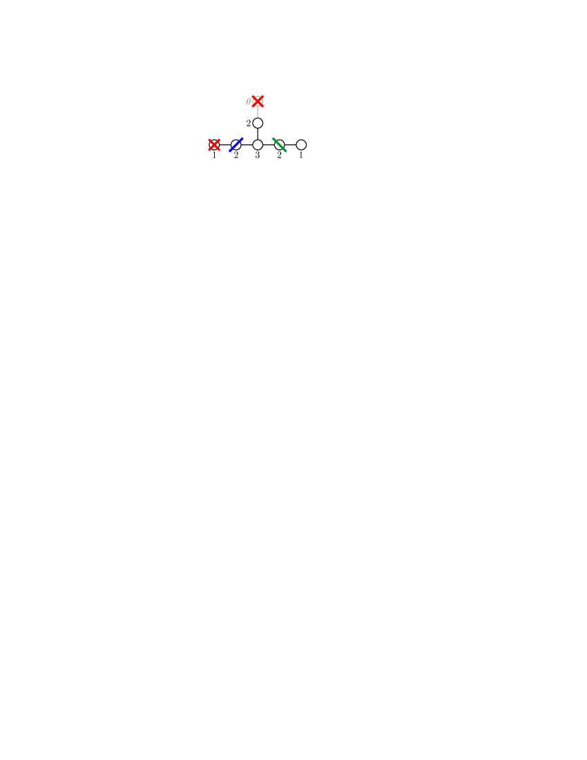
Figure 2: $\mathrm{E}_{6}$ breaking patterns under $\mathbbm{Z}_{2}$ twisting. Three different $\mathbbm{Z}_{2}$ twists are indicated by crosses, a slash and a backslash, respectively.

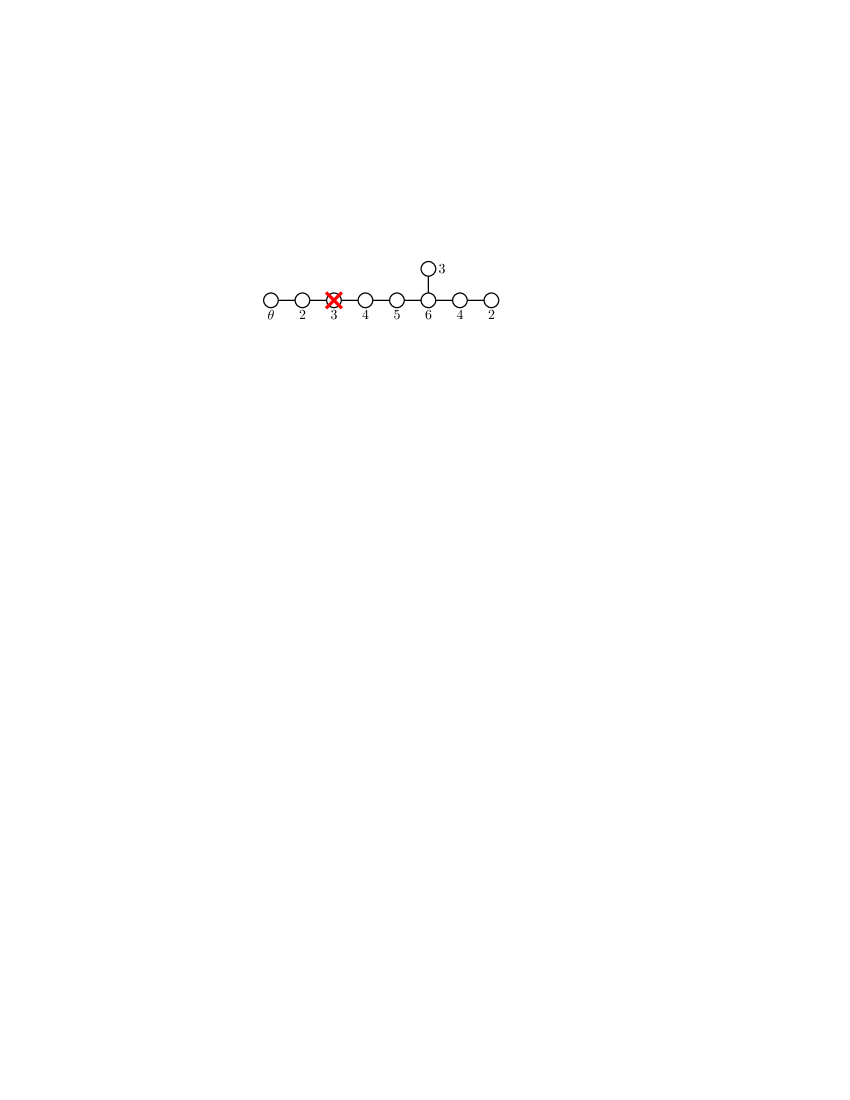
Figure 3: $\mathrm{E}_{8}$ breaking to $\mathrm{E}_{6}\times\mathrm{SU}(3)$.

As in the $\mathrm{SO}(10)$ example, one can check that the same breaking can be obtained as an intersection of three different $\mathrm{SO}(10)$ embeddings in $\mathrm{E}_{6}$ which correspond to the twists

$$\mathrm{E}_{6}\xrightarrow{P_{A}\cdot P_{C}}\mathrm{SO}(10)^{\prime}\times\mathrm{U}(1)^{\prime}\;,\quad\mathrm{E}_{6}\xrightarrow{P_{A}\cdot P_{B}\cdot P_{C}}\mathrm{SO}(10)^{\prime\prime}\times\mathrm{U}(1)^{\prime\prime}\;,$$ (10)

such that

$$\mathrm{SO}(10)\times\mathrm{U}(1)\ \cap\ \mathrm{SO}(10)^{\prime}\times\mathrm{U}(1)^{\prime}\ \cap\ \mathrm{SO}(10)^{\prime\prime}\times\mathrm{U}(1)^{\prime\prime}\\ =\ \mathrm{SU}(3)\times\mathrm{SU}(2)\times\mathrm{U}(1)^{2}\ \sim\ G_{\mathrm{SM}}\;.$$ (11)

Let us remark that it is not possible to distinguish the three $\mathrm{SO}(10)$ embeddings in $\mathrm{E}_{6}$ (as well as $G_{\mathrm{GG}}$ and $G_{\mathrm{fl}}$ embeddings in $\mathrm{SO}(10)$) at the level of Dynkin diagrams. The corresponding subalgebras are related by Weyl reflections within the embedding group. To distinguish them, an explicit analysis of the shift vectors $V_{N}$ is required.

Our final goal is to break $\mathrm{E}_{8}$ to the standard model gauge group. This can be achieved by combining the above three $\mathbbm{Z}_{2}$ twists with a $\mathbbm{Z}_{3}$ twist which breaks $\mathrm{E}_{8}$ to $\mathrm{E}_{6}\times\mathrm{SU}(3)$ (cf. Fig. 3). The $\mathbbm{Z}_{2}$ twists can then also break the $\mathrm{SU}(3)$ factor to $\mathrm{SU}(2)\times\mathrm{U}(1)$. In this way one obtains three $\mathbbm{Z}_{6}$ twists which break $\mathrm{E}_{8}$ to subgroups containing $\mathrm{SO}(10)$,

$$\mathrm{E}_{8} \stackrel{{\scriptstyle P_{6}}}{{\longrightarrow}} \mathrm{SO}(10)\times\mathrm{SU}(3)\times\mathrm{U}(1)\;,\quad\mathrm{E}_{8}\,\stackrel{{\scriptstyle P_{6}^{\prime}}}{{\longrightarrow}}\,\mathrm{SO}(10)^{\prime}\times\mathrm{SU}(2)^{\prime}\times\mathrm{U}(1)^{2}\;,$$

$$\mathrm{E}_{8} \stackrel{{\scriptstyle P_{6}^{\prime\prime}}}{{\longrightarrow}} \mathrm{SO}(10)^{\prime\prime}\times\mathrm{SU}(2)^{\prime\prime}\times\mathrm{U}(1)^{2}\;,$$ (12)

such that the intersection is the standard model group up to $\mathrm{U}(1)$ factors,

$$\mathrm{SO}(10)\times\mathrm{SU}(3)\times\mathrm{U}(1)\ \cap\ \mathrm{SO}(10)^{\prime}\times\mathrm{SU}(2)^{\prime}\times\mathrm{U}(1)^{2}\\ \cap\ \mathrm{SO}(10)^{\prime\prime}\times\mathrm{SU}(2)^{\prime\prime}\times\mathrm{U}(1)^{2}\ \sim\ G_{\mathrm{SM}}\;.$$ (13)

In an orthonormal basis of $\mathrm{E}_{8}$ roots, three $\mathbbm{Z}_{6}$ shift vectors which realize the described symmetry breaking read explicitly:

$$V_{6} = \left({1\over 3},{1\over 3},{1\over 3},0,0,0,0,0\right)\;,$$

$$V_{6}^{\prime} = \left({7\over 12},{7\over 12},{1\over 12},{1\over 4},-{1\over 4},-{3\over 4},-{3\over 4},-{3\over 4}\right)\;,$$

$$V_{6}^{\prime\prime} = \left({7\over 12},{13\over 12},{7\over 12},{3\over 4},{1\over 4},-{3\over 4},-{3\over 4},-{3\over 4}\right)\;.$$ (14)

Note that the differences between the $\mathbbm{Z}_{6}$ shift vectors are $\mathbbm{Z}_{2}$ shift vectors,

$$W_{2} = V_{6}^{\prime\prime}-V_{6}^{\prime}=\left(0,{1\over 2},{1\over 2},{1\over 2},{1\over 2},0,0,0\right)\;,$$

$$W_{2}^{\prime} = V_{6}^{\prime}-V_{6}=\left({1\over 4},{1\over 4},-{1\over 4},{1\over 4},-{1\over 4},-{3\over 4},-{3\over 4},-{3\over 4}\right)\;,$$ (15)

which will play the role of Wilson lines in the next section.

To summarize, in this section we have presented a group–theoretical analysis of $\mathrm{E}_{8}$ breaking to the standard model with intermediate $\mathrm{E}_{6}$ and $\mathrm{SO}(10)$ GUTs, suggested by the structure of matter multiplets.

2 Orbifold compactification

Let us now construct an orbifold compactification of the heterotic string, which realizes the symmetry breaking described above. As is clear from the above discussion, we will need a $\mathbbm{Z}_{6}$ or a higher–order orbifold and choose the former for simplicity.

In the light cone gauge the heterotic string [6] can be described by the following bosonic world sheet fields: 8 string coordinates $X^{i}$, $i=1\ldots 8$, 16 internal left-moving coordinates $X^{I}$, $I=1\ldots 16$, and 4 right-moving fields $\phi^{i}$, $i=1\ldots 4$, which correspond to the bosonized Neveu-Schwarz-Ramond fermions (cf. [20, 16, 21]). The 16 left-moving internal coordinates are compactified on a torus. The associated quantized momenta lie on the $\mathrm{E}_{8}\times\mathrm{E}_{8}$ root lattice. In an orthonormal basis, vectors of the $\mathrm{E}_{8}$ root lattice are given by

$$p_{{}_{\mathrm{E}_{8}}}=(n_{1},...,n_{8})\;\;{\rm or}\;\;\left(n_{1}+{1\over 2},...,n_{8}+{1\over 2}\right)\;,$$ (16)

with integer $n_{i}$ satisfying $\sum_{i=1}^{8}n_{i}=0\mod 2$. The massless spectrum of this 10D string is 10D supergravity coupled to $\mathrm{E}_{8}\times\mathrm{E}_{8}$ super Yang–Mills theory.

To obtain a four–dimensional theory, 6 dimensions of the 10D heterotic string are compactified on an orbifold. In our case, this is a $\mathbbm{Z}_{6}$ orbifold obtained by modding a 6D torus together with the 16D gauge torus by a $\mathbbm{Z}_{6}$ twist,

$${\cal O}\ =\ T^{6}\otimes T_{\mathrm{E}_{8}\times\mathrm{E}_{8}^{\prime}}/\mathbbm{Z}_{6}\;.$$ (17)

On the three complex torus coordinates $z^{i}$, $i=1,2,3$, the $\mathbbm{Z}_{6}$ twist acts as

$$z^{i}\rightarrow e^{2\pi\mathrm{i}\,v_{6}^{i}}\leavevmode\nobreak\ z^{i}\;.$$ (18)

Here $6v_{6}$ has integer components. The compact string coordinates are described by the complex variables $Z^{i}=X^{2i-1}+\mathrm{i}\ X^{2i}$, $i=1\ldots 3$. The $\mathbbm{Z}_{6}$ action on the string coordinates reads, up to lattice translations (cf. [16]),

$$Z^{i}(\sigma=2\pi)=e^{2\pi\mathrm{i}kv_{6}^{i}}\ Z^{i}(\sigma=0)\;,\quad k=0\ldots 5\;,$$ (19)

$$\phi^{i}(\sigma=2\pi)=\phi^{i}(\sigma=0)-\pi kv_{6}^{i}\;,\quad X^{I}(\sigma=2\pi)=X^{I}(\sigma=0)+\pi kV_{6}^{I}\;,$$ (20)

where $6V^{I}$ is an $\mathrm{E}_{8}\times\mathrm{E}_{8}$ lattice vector.

The torus $T^{6}$ is spanned by basis vectors $e_{\kappa}$, $\kappa=1,...,6$. In general, a torus allows for the presence of Wilson lines, i.e. a translation by a lattice vector $n_{\kappa}e_{\kappa}^{i}$ can be accompanied by a shift of the internal string coordinates,

$$X^{i}(\sigma=2\pi) = X^{i}(\sigma=0)+2\pi n_{\kappa}e_{\kappa}^{i}\;,\quad n_{\kappa}\in\mathbbm{Z}\;,$$

$$X^{I}(\sigma=2\pi) = X^{I}(\sigma=0)+\pi n_{\kappa}W_{\kappa}^{I}\;.$$ (21)

Here the discrete Wilson lines $W_{\kappa}$ are restricted by symmetry and by modular invariance.

The basis vectors $e_{\kappa}$ are taken to be simple roots of a Lie algebra, whose choice is dictated by the required symmetry of the lattice. In our case the lattice must have a $\mathbbm{Z}_{6}$ symmetry and allow for the existence of 3 independent $V_{6}$ shift vectors (14) (or two Wilson lines of order 2). This leaves two possibilities for the Lie lattice [16]:

$$\mathrm{G}_{2}\times\mathrm{SU}(3)\times\mathrm{SO}(4)\;\;{\rm or}\;\;\mathrm{SU}(3)^{[2]}\times\mathrm{SU}(3)\times\mathrm{SO}(4)\;.$$ (22)

We shall base our analysis on the first lattice, which has recently been studied in detail by Kobayashi, Raby and Zhang [12]. These authors have obtained models with the Pati-Salam gauge group in four dimensions, which then has to be broken to the standard model by the Higgs mechanism. The model described in the following differs from those in the choice of $\mathbbm{Z}_{6}$ twists and the pattern of symmetry breaking.

For the $\mathrm{G}_{2}\times\mathrm{SU}(3)\times\mathrm{SO}(4)$ lattice, the action of the $\mathbbm{Z}_{6}$ twist is given by Eq. (18) with

$$v_{6}={1\over 6}(1,2,-3)\;.$$ (23)

$z_{1}$, $z_{2}$ and $z_{3}$ are the coordinates of the $\mathrm{G}_{2}$, $\mathrm{SU}(3)$ and $\mathrm{SO}(4)$ $T^{2}$-tori, respectively. The $\mathbbm{Z}_{6}$ twist $v_{6}$ has two subtwists,

$$\mathbbm{Z}_{3}:\;v_{3}=2v_{6}={1\over 3}(1,2,-3)\;,\quad\mathbbm{Z}_{2}:\;v_{2}=3v_{6}={1\over 2}(1,2,-3)\;.$$ (24)

An interesting feature of this orbifold is the occurrence of invariant planes. Clearly, the $\mathbbm{Z}_{3}$ twist leaves the $\mathrm{SO}(4)$-plane invariant whereas the $\mathbbm{Z}_{2}$ twist leaves the $\mathrm{SU}(3)$-plane invariant. The corresponding fixed points and invariant planes are shown in Fig. 4. Our construction requires two Wilson lines in the $\mathrm{SO}(4)$ plane, $W_{2}$ and $W_{2}^{\prime}$, such that there are 3 independent gauge shift vectors (14) acting at different fixed points in this plane.

$\mathrm{G}_{2}$ torus $\mathrm{SU}(3)$ torus $\mathrm{SO}(4)$ torus $\mathbbm{Z}_{6}\leavevmode\nobreak\ ;\leavevmode\nobreak\ T_{1,5}$ $\mathbbm{Z}_{3}\leavevmode\nobreak\ ;\leavevmode\nobreak\ T_{2,4}$ $\mathbbm{Z}_{2}\leavevmode\nobreak\ ;\leavevmode\nobreak\ T_{3}$

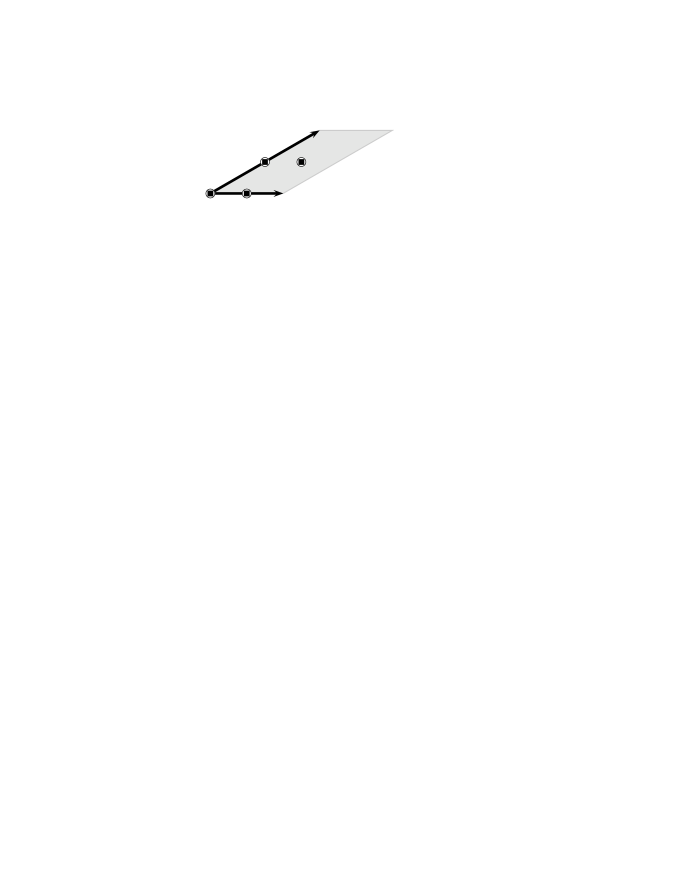
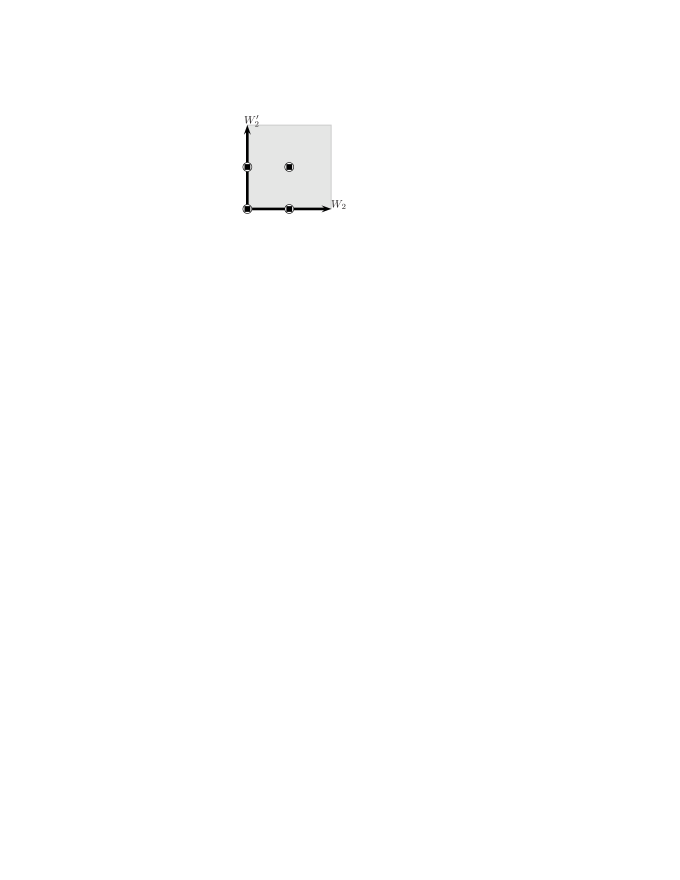
Figure 4: Fixed points and invariant planes (hatched) under the $\mathbbm{Z}_{6}$ twist and $\mathbbm{Z}_{3},\mathbbm{Z}_{2}$ subtwists, describing localization of different twisted sectors.

The rules of orbifold compactifications of the heterotic string have recently been reviewed in [13, 14]. We are interested in the states whose masses are small compared to the string scale $M_{S}$. These states are described by fields

$$\Psi_{r,s}(x;z_{1},z_{2},z_{3})\;.$$ (25)

Here $r$ labels the gauge quantum numbers and is given by

$$r\,=\left\{\begin{array}[]{ll}p&\text{for the untwisted sector}\;,\\ p+k\,V_{6}&\text{for the}\>k\text{-th twisted sector}\;,\end{array}\right.$$ (26)

where $p$ lies on the $\mathrm{E}_{8}\times\mathrm{E}_{8}$ root lattice (16) and we have absorbed the Wilson lines in the definition of the $local$ twist $kV_{6}$. Similarly, $s$ carries information about the spin,

$$s\,=\left\{\begin{array}[]{ll}q&\text{for the untwisted sector}\;,\\ q+k\,v_{6}&\text{for the}\>k\text{-th twisted sector}\;,\end{array}\right.$$ (27)

where $q$ is an element of the $\mathrm{SO}(8)$ weight lattice and $v_{6}^{4}=0$. In our convention, the last component of $q$ gives the 4D helicity. For example, 4D vectors correspond to $q=(0,0,0,\pm 1)$, 4D scalars to $q=(\pm 1,0,0,0)$ with all permutations of the first 3 entries, and fermions correspond to $q=\left(\pm{1\over 2},\pm{1\over 2},\pm{1\over 2},\pm{1\over 2}\right)$ with an even number of ‘+’ signs.

The physical states are invariant under the action of the orbifold symmetry group which consists of twists and translations. In our case only translations in the $\mathrm{SO}(4)$ plane have a non–trivial action on the gauge degrees of freedom, due to the presence of Wilson lines. Then the invariance conditions read ($\ell=1,...,5$):

$$\Psi_{r,s}(x;z_{1},z_{2},z_{3}) = e^{2\pi\mathrm{i}\,\ell(r\cdot V_{6}-s\cdot v_{6})}\Psi_{r,s}\left(x;e^{2\pi\mathrm{i}{\ell\over 6}}z_{1},e^{2\pi\mathrm{i}{\ell\over 3}}z_{2},e^{-2\pi\mathrm{i}{\ell\over 2}}z_{3}\right),$$

$$\Psi_{r,s}(x;z_{1},z_{2},z_{3}) = e^{2\pi\mathrm{i}\,r\cdot W_{2}}\Psi_{r,s}\left(x;z_{1},z_{2},z_{3}+1\right)\;,$$

$$\Psi_{r,s}(x;z_{1},z_{2},z_{3}) = e^{2\pi\mathrm{i}\,r\cdot W_{2}^{\prime}}\Psi_{r,s}\left(x;z_{1},z_{2},z_{3}+\mathrm{i}\right)\;,$$ (28)

where we have included the Wilson lines in the local shift vectors $kV_{6}$. We note that here two sources of symmetry breaking are present: local, due to twisting, and non-local, due to the Wilson lines. In the first case, symmetry breaking is restricted to the fixed points in the compact space. Indeed, since orbifold fixed points are invariant under twisting (up to a lattice vector), the first condition can be satisfied only for certain $p$, which indicates symmetry breaking at the fixed points. These sets of $p$’s are generally different at different fixed points and only their intersection survives in 4D, since in this case the wave function can be constant in the compactified dimensions leading to a massless state. In the case of Wilson line symmetry breaking, the second and third conditions apply to all points in the $\mathrm{G}_{2}$ and $\mathrm{SU}(3)$ planes and the symmetry breaking is non-local.

To define our string model, it is necessary to specify the action of the twist on the second, ‘hidden’, $\mathrm{E}_{8}$. We find that the desired symmetry breaking pattern and the appearance of three $\boldsymbol{16}$-plets at fixed points with unbroken $\mathrm{SO}(10)$ lead to

$$V_{6} = \left({1\over 3},{1\over 3},{1\over 3},0,0,0,0,0\right)\left({1\over 6},{1\over 6},0,0,0,0,0,0\right)\;,$$ (29)

$$W_{2} = \left(0,{1\over 2},{1\over 2},{1\over 2},{1\over 2},0,0,0\right)\left({1\over 2},{1\over 2},{1\over 2},0,0,0,0,{1\over 2}\right)\;,$$ (30)

$${W_{2}}^{\prime} = \left({1\over 4},{1\over 4},-{1\over 4},{1\over 4},-{1\over 4},-{3\over 4},-{3\over 4},-{3\over 4}\right)\left(0,{1\over 2},{1\over 2},{1\over 2},{1\over 2},0,0,0\right)\;$$ (31)

in the orthonormal $\mathrm{E}_{8}\times\mathrm{E}_{8}$ basis. In string theory, these quantities must satisfy certain consistency conditions (see [13] for a recent discussion). First of all, $6V_{6}$ and $2W_{2},2W_{2}^{\prime}$ must be elements of the $\mathrm{E}_{8}\times\mathrm{E}_{8}$ root lattice which is required by embedding of the orbifold symmetry group (‘space’ group) in the gauge degrees of freedom. Second, modular invariance requires

$$6\left[(mV_{6}+nW_{2}+n^{\prime}W_{2}^{\prime})^{2}-m^{2}v_{6}^{2}\right]=0{\rm\leavevmode\nobreak\ mod\leavevmode\nobreak\ 2},\leavevmode\nobreak\ \leavevmode\nobreak\ m,n,n^{\prime}=0,1\;.$$ (32)

Our choice of the hidden sector components of $V_{6},W_{2},W_{2}^{\prime}$ is strongly affected by these conditions.

We note that $N=1$ supersymmetry in 4D requires

$$\sum_{i=1}^{3}v_{6}^{i}=0{\rm\leavevmode\nobreak\ mod\leavevmode\nobreak\ 1}\;,$$ (33)

whereas $N=2$ would require, in addition, $v_{6}^{i}=0$ mod 1 for some $i$. In the former case, there is one gravitino satisfying $q\cdot v_{6}=0$ mod 1 whereas in the latter case there are two of them.

Finally, massless states in 4D must satisfy the following conditions:

$$q^{2}=1\leavevmode\nobreak\ \leavevmode\nobreak\ ,\leavevmode\nobreak\ \leavevmode\nobreak\ p^{2}=2-2\tilde{N}$$ (34)

for the untwisted sector, and

$$(q+kv_{6})^{2}=c_{k}\leavevmode\nobreak\ \leavevmode\nobreak\ ,\leavevmode\nobreak\ \leavevmode\nobreak\ \bigl{(}p+kV_{6}+nW_{2}+n^{\prime}W_{2}^{\prime}\bigr{)}^{2}=c_{k,\tilde{N}}$$ (35)

for the $k$-th twisted sector. Here $\tilde{N}$ is an oscillator number and $c_{k},c_{k,\tilde{N}}$ are certain constants (see e.g. [13]). In our model, all states which transform non–trivially under $\mathrm{SU}(3)_{c}\times\mathrm{SU}(2)_{\mathrm{L}}$ have $\tilde{N}=0$.

In this section we have described the necessary ingredients of our orbifold model. In the next section we compute the massless spectrum of the model and discuss localization of various states.

3 Massless spectrum of the model

First let us identify the gauge group in 4D. For $N=1$ vector multiplets $q\cdot v_{6}=0$. Hence, the surviving gauge group in 4D is given by the root vectors satisfying

$$p\cdot V_{6},\ p\cdot W_{2},\ p\cdot W_{2}^{\prime}\ \in\mathbbm{Z}\;,\quad p^{2}=2\;.$$ (36)

It is straightforward to verify that these roots together with the Cartan generators form the Lie algebra of

$$\mathrm{SU}(3)\times\mathrm{SU}(2)\times\mathrm{U}(1)^{5}\leavevmode\nobreak\ \leavevmode\nobreak\ ,$$

while the hidden sector $\mathrm{E}_{8}$ is broken to $\mathrm{SU}(4)\times\mathrm{SU}(4)\times\mathrm{U}(1)^{2}$. This result can be understood by examining the enhanced gauge groups at the four orbifold fixed points in the $\mathrm{SO}(4)$-plane. These gauge groups are determined by

$$p\vspace{2cm}\cdot\Bigl{(}V_{6}+nW_{2}+n^{\prime}W_{2}^{\prime}\Bigr{)}\in\mathbbm{Z}\;,$$ (37)

where $n,n^{\prime}=\{0,1\}$ specify the fixed point in the $\mathrm{SO}(4)$ plane. Then, omitting the hidden sector the local gauge groups are (Fig. 5):

$$(n=0,n^{\prime}=0):\leavevmode\nobreak\ \mathrm{SO}(10)\times\mathrm{SU}(3)\times\mathrm{U}(1)$$

$$(n=1,n^{\prime}=0):\leavevmode\nobreak\ \mathrm{SU}(6)\times\mathrm{SU}(2)\times\mathrm{SU}(2)\times\mathrm{U}(1)$$

$$(n=0,n^{\prime}=1):\leavevmode\nobreak\ \mathrm{SO}(10)\times\mathrm{SU}(2)\times\mathrm{U}(1)^{2}$$

$$(n=1,n^{\prime}=1):\leavevmode\nobreak\ \mathrm{SO}(10)\times\mathrm{SU}(2)\times\mathrm{U}(1)^{2}\;.$$ (38)

These are precisely the groups discussed in the first section. Their intersection yields the surviving group $\mathrm{SU}(3)\times\mathrm{SU}(2)\times\mathrm{U}(1)^{5}$.

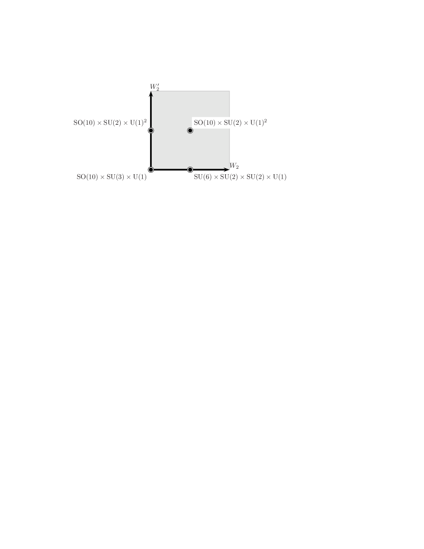
Figure 5: Local gauge symmetries in the $\mathrm{SO}(4)$-plane.

Let us now consider matter fields. These can be either in the untwisted sector $U$ or in one of the twisted sectors $T_{1}\ldots T_{5}$. Below we analyze each of them separately. Before we proceed, let us fix the chirality of the matter fields to be $positive$, i.e. $q_{4}=+1/2$ for their fermionic components.

3.1 $\boldsymbol{U}$ sector

For $N=1$ chiral multiplets in the untwisted sector we have $q\cdot v_{6}=\pm 1/6$, $\pm 1/3$, $\pm 1/2$, and therefore

$$p\cdot V_{6}=\{1/6,1/3,1/2\}\leavevmode\nobreak\ {\rm mod}\leavevmode\nobreak\ 1\;;\quad p\cdot W_{2},\ p\cdot W_{2}^{\prime}\ \in\mathbbm{Z}\;.$$ (39)

The states represent bulk matter of the orbifold. By choosing an appropriate right–mover, these massless states can be made invariant under the $\mathbbm{Z}_{6}$ orbifold action and thus are present in the 4D spectrum. Apart from $\mathrm{SU}(3)_{c}\times\mathrm{SU}(2)_{\mathrm{L}}$ singlets, the untwisted sector of our model contains

$$U=2\times(\boldsymbol{3},\boldsymbol{1})\oplus(\bar{\boldsymbol{3}},\boldsymbol{1})\oplus 5\times(\boldsymbol{1},\boldsymbol{2})$$ (40)

in terms of the $\mathrm{SU}(3)_{c}\times\mathrm{SU}(2)_{\mathrm{L}}$ quantum numbers. From the field-theory perspective, these fields correspond to the compact space components of the $E_{8}$ gauge fields and their superpartners.

3.2 $\boldsymbol{T_{1}+T_{5}}$ sector

These matter fields are located at the 12 orbifold fixed points (Fig. 4) and satisfy

$$\Bigl{(}p+V_{6}+nW_{2}+n^{\prime}W_{2}^{\prime}\Bigr{)}^{2}={25\over 18}\;.$$ (41)

Since Wilson lines are present only in the $\mathrm{SO}(4)$ plane, only $\mathrm{SO}(4)$-plane projections of the fixed points matter. The $\mathrm{G}_{2}$ and $\mathrm{SU}(3)$ projections do not affect the local twist. They only lead to a multiplicity factor 3 due to the three identical $\mathrm{SU}(3)$ fixed points. Any massless state in the $T_{1}$ sector survives the orbifold projection, i.e. is invariant under the $\mathbbm{Z}_{6}$ action, and is therefore present in the 4D spectrum.

The twisted matter fields located at a given fixed point appear in a representation of the local gauge group at this point. In our case, twisted matter with $\mathrm{SU}(3)_{c}\times\mathrm{SU}(2)_{\mathrm{L}}$ quantum numbers is

$$(n=0,n^{\prime}=0):\leavevmode\nobreak\ 3\times(\overline{\boldsymbol{16}},1)$$

$$(n=1,n^{\prime}=0):\leavevmode\nobreak\ 6\times(1,\boldsymbol{2},1)$$

$$(n=0,n^{\prime}=1):\leavevmode\nobreak\ -$$

$$(n=1,n^{\prime}=1):\leavevmode\nobreak\ -$$ (42)

It is convenient to keep the notation $(\overline{\boldsymbol{16}})$ of $\mathrm{SO}(10)$ even though the unbroken group in 4D is only $G_{\mathrm{SM}}$, since it represents one complete generation of SM fermions including right–handed neutrinos. In terms of $\mathrm{SU}(3)_{c}\times\mathrm{SU}(2)_{\mathrm{L}}$ quantum numbers we have

$$T_{1}+T_{5}=3\times(\overline{\boldsymbol{16}})\oplus 6\times(\boldsymbol{1},\boldsymbol{2})\;,$$ (43)

where again we have omitted singlets.

3.3 $\boldsymbol{T_{2}+T_{4}}$ sector

These states are localized at the fixed points in the $\mathrm{G}_{2}$ and $\mathrm{SU}(3)$ planes, while being bulk states in the $\mathrm{SO}(4)$ plane (Fig. 4). If the $T_{1}$ sector corresponds to the string with the boundary condition twisted by $\Theta=\operatorname{diag}\left(e^{2\pi\mathrm{i}\,v_{6}^{1}},e^{2\pi\mathrm{i}\,v_{6}^{2}},e^{2\pi\mathrm{i}\,v_{6}^{3}}\right)$, the $T_{2}$ sector corresponds to the strings twisted by $\Theta^{2}$. Since $\Theta^{2}$ has a fixed plane, $T_{2}$ states are bulk states in this plane and localized states in the other two planes.

The orbifold action on this sector is $\mathbbm{Z}_{3}$, and is given by

$$v_{3}=2v_{6}\leavevmode\nobreak\ \leavevmode\nobreak\ ,\leavevmode\nobreak\ \leavevmode\nobreak\ V_{3}=2V_{6}\leavevmode\nobreak\ \;.$$ (44)

Since there are no Wilson lines in the $\mathrm{G}_{2}$ and $\mathrm{SU}(3)$ planes, all fixed points are equivalent. The massless $N=1$ multiplets obey

$$\Bigl{(}p+V_{3}\Bigr{)}^{2}={14\over 9}\;.$$ (45)

Both the $\mathrm{G}_{2}$ and the $\mathrm{SU}(3)$ lattice have 3 fixed points under $\mathbbm{Z}_{3}$, so the multiplicity factor is 9. The local gauge groups at the fixed points are determined by

$$p\cdot V_{3}=0\;.$$ (46)

At each $\mathbbm{Z}_{3}$ fixed point, the unbroken gauge group and the twisted sector matter fields are (cf. Fig. 6)

$$\mathrm{E}_{6}\times\mathrm{SU}(3):\quad(\overline{\boldsymbol{27}},1)\;,$$ (47)

plus $\mathrm{SU}(3)_{c}\times\mathrm{SU}(2)_{\mathrm{L}}$ singlets.

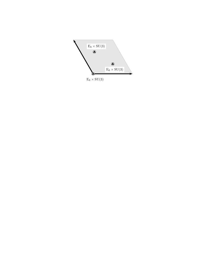
Figure 6: Local gauge symmetries in the $\mathrm{SU}(3)$-plane after the $\mathbbm{Z}_{3}$ subtwist.

These states are subject to further projection and not all of them survive. Indeed, by construction they are only invariant under the $\mathbbm{Z}_{3}$ action, but not under the full $\mathbbm{Z}_{6}$. Furthermore, the $\mathbbm{Z}_{3}$ fixed points in the $\mathrm{G}_{2}$-plane are only fixed under $\mathbbm{Z}_{3}$ and the $\mathbbm{Z}_{6}$ action transforms them into one another. Physical states are formed out of their linear combinations which are eigenstates of the $\mathbbm{Z}_{6}$ twist.

The $\mathbbm{Z}_{3}$ invariance of a physical state requires

$$(q+v_{3})\cdot v_{3}=(p+V_{3})\cdot V_{3}{\rm\leavevmode\nobreak\ mod\leavevmode\nobreak\ }1\;,$$ (48)

where $q+v_{3}$ is the shifted $\mathrm{SO}(8)$ momentum and $p+V_{3}$ is the shifted $\mathrm{E}_{8}\times\mathrm{E}_{8}$ momentum. This is satisfied automatically as long as the gauge embedding of the twist and the Wilson lines obey modular invariance (yet it may require shifts by a lattice vector). A non-trivial $\mathbbm{Z}_{2}$ invariance condition is

$$(q+v_{3})\cdot v_{2}=(p+V_{3})\cdot V_{2}\leavevmode\nobreak\ +\leavevmode\nobreak\ \gamma{\rm\leavevmode\nobreak\ mod\leavevmode\nobreak\ }1\;,\quad p\cdot W_{2},\ p\cdot W_{2}^{\prime}\ \in\mathbbm{Z}\;,$$ (49)

where

$$v_{2}=3v_{6}\leavevmode\nobreak\ \leavevmode\nobreak\ ,\leavevmode\nobreak\ \leavevmode\nobreak\ V_{2}=3V_{6}\;.$$ (50)

The extra term $\gamma=(0,0,1/2)$ appears due to the “mixing” of the fixed points [22],[12]. There are three combinations of the $\mathbbm{Z}_{3}$ fixed points which are eigenstates of $\mathbbm{Z}_{6}$ with eigenvalues $e^{2\pi\mathrm{i}\gamma}$.

An important note is in order. The $\mathrm{SO}(8)$ lattice momentum $q$ is found via the masslessness condition for the right–movers,

$$(q+v_{3})^{2}={5\over 9}\;.$$ (51)

Since $v_{3}$ has a fixed plane, there are always two sets of solutions, with opposite chiralities. Both of them survive the projection (48), which leads to $N=2$ hypermultiplets. The conditions (49) break the symmetry between the two chiralities and one obtains $N=1$ chiral multiplets.

As a result, $9\times(\overline{\boldsymbol{27}})$ $N$=$2$ hypermultiplets produce the following $N$=$1$ multiplets with $\mathrm{SU}(3)_{c}\times\mathrm{SU}(2)_{\mathrm{L}}$ quantum numbers:

$$T_{2}+T_{4}=3\times(\boldsymbol{3},\boldsymbol{1})\oplus 6\times(\bar{\boldsymbol{3}},\boldsymbol{1})\oplus 9\times(\boldsymbol{1},\boldsymbol{2})\;.$$ (52)

3.4 $\boldsymbol{T_{3}}$ sector

These states are localized at the $\mathbbm{Z}_{2}$ fixed points in the $\mathrm{G}_{2}$ and $\mathrm{SO}(4)$ planes and are bulk states in the $\mathrm{SU}(3)$ plane (Fig. 4). They correspond to strings twisted by $\Theta^{3}$. The massless $T_{3}$ states satisfy

$$\Bigl{(}p+V_{2}+nW_{2}+n^{\prime}W_{2}^{\prime}\Bigr{)}^{2}={3\over 2}\;,$$ (53)

and the local gauge groups at the fixed points are determined by

$$p\cdot\Bigl{(}V_{2}+nW_{2}+n^{\prime}W_{2}^{\prime}\Bigr{)}=0\;.$$ (54)

The result for gauge groups and matter multiplets reads

$$(n=0,n^{\prime}=0):\leavevmode\nobreak\ \mathrm{SO}(16)\leavevmode\nobreak\ ,\leavevmode\nobreak\ 8\times(\boldsymbol{16})$$

$$(n=1,n^{\prime}=0):\leavevmode\nobreak\ \mathrm{SO}(16)\leavevmode\nobreak\ ,\leavevmode\nobreak\ 8\times(\boldsymbol{16})$$

$$(n=0,n^{\prime}=1):\leavevmode\nobreak\ \mathrm{E}_{7}\times\mathrm{SU}(2)\leavevmode\nobreak\ ,\leavevmode\nobreak\ -$$

$$(n=1,n^{\prime}=1):\leavevmode\nobreak\ \mathrm{E}_{7}\times\mathrm{SU}(2)\leavevmode\nobreak\ ,\leavevmode\nobreak\ -\quad.$$ (55)

As usual we have omitted $\mathrm{SU}(3)_{c}\times\mathrm{SU}(2)_{\mathrm{L}}$ singlets and included a multiplicity factor 4 from the $\mathrm{G}_{2}$-plane fixed points. These states are located at the $\mathbbm{Z}_{2}$ fixed points which are mixed by the action of the full $\mathbbm{Z}_{6}$ twist. Again, one has to form linear combinations of the states transforming covariantly under $\mathbbm{Z}_{6}$.

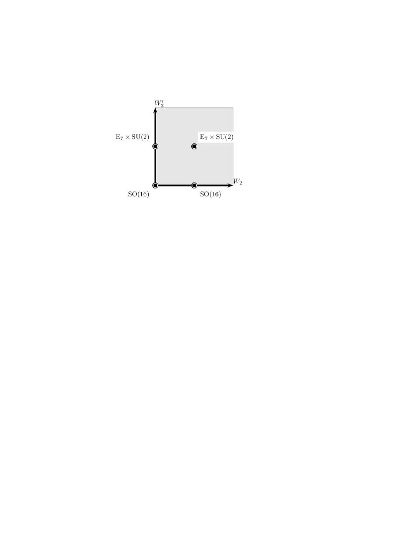
Figure 7: Local gauge symmetries in the $\mathrm{SO}(4)$-plane after the $\mathbbm{Z}_{2}$ subtwist.

The matter states are, as before, subject to projection conditions. The $\mathbbm{Z}_{2}$ condition for the relevant states is

$$(q+v_{2})\cdot v_{2}=(p+V_{2}+nW_{2})\cdot(V_{2}+nW_{2}){\rm\leavevmode\nobreak\ mod\leavevmode\nobreak\ }1\;.$$ (56)

With a proper redefinition of $W_{2}$ by a lattice vector shift, this condition is satisfied by all states with both chiralities, i.e. both solutions $q$ of the equation for massless right–movers,

$$(q+v_{2})^{2}={1\over 2}\;.$$ (57)

Therefore, these states form $N=2$ hypermultiplets. The further $\mathbbm{Z}_{3}$ projection reads

$$(q+v_{2})\cdot v_{3}=(p+V_{2}+nW_{2})\cdot V_{3}\leavevmode\nobreak\ +\leavevmode\nobreak\ \gamma{\rm\leavevmode\nobreak\ mod\leavevmode\nobreak\ }1\;,$$ (58)

where now $\gamma=(0,0,1/3,-1/3)$. The four $\mathbbm{Z}_{2}$ fixed points in the $\mathrm{G}_{2}$-plane lead to four eigenstates under $\mathbbm{Z}_{3}$ with eigenvalues $e^{2\pi\mathrm{i}\gamma}$. The above condition projects out some of the states. The surviving $N$=1 multiplets with $\mathrm{SU}(3)_{c}\times\mathrm{SU}(2)_{\mathrm{L}}$ quantum numbers are

$$T_{3}=7\times(\boldsymbol{3},\boldsymbol{1})\oplus 5\times(\bar{\boldsymbol{3}},\boldsymbol{1})\oplus 10\times(\boldsymbol{1},\boldsymbol{2})\;.$$ (59)

3.5 Summary of the massless spectrum

Combining all matter multiplets from the untwisted and the five twisted sectors we finally obtain

$$M = U+T_{1}+T_{2}+T_{3}+T_{4}+T_{5}$$ (60)

$$= 3\times({\overline{\boldsymbol{16}}})\oplus 12\times(\boldsymbol{3},\boldsymbol{1})\oplus 12\times(\bar{\boldsymbol{3}},\boldsymbol{1})\oplus 30\times(\boldsymbol{1},\boldsymbol{2})\;,$$

plus $\mathrm{SU}(3)_{c}\times\mathrm{SU}(2)_{\mathrm{L}}$ singlets. Note that in addition to three SM generations contained in the three ${\bf 16}$-plets we have only vector–like matter. This result is partly dictated by the requirement of anomaly cancellations. Vector–like fields can attain large masses and decouple from the low energy theory. A detailed analysis of this issue, including $\mathrm{U(1)}$ factors, will be presented in a subsequent publication.

4 Intermediate GUTs

So far we have made no assumption on the size of the compact dimensions. These are usually assumed to be given by the string scale, $R_{i}\sim 1/M_{S}$. However, this is not necessarily the case and, furthermore, unification of the gauge couplings favours anisotropic compactifications where some of the radii are significantly larger than the others [23, 24]. In this case one encounters a higher–dimensional GUT at an intermediate energy scale. Indeed, the Kaluza–Klein modes associated with a large dimension of radius $R$ become light and are excited at energy scales above $1/R\ll M_{S}$. At these energy scales we obtain an effective higher–dimensional field theory with enhanced symmetry in the bulk.

In our model there are four independent radii: two are associated with the $\mathrm{G}_{2}$ and $\mathrm{SU}(3)$ planes, respectively, and the other two are associated with the two independent directions in the $\mathrm{SO}(4)$-plane. Any of these radii can in principle be large leading to a distinct GUT model.

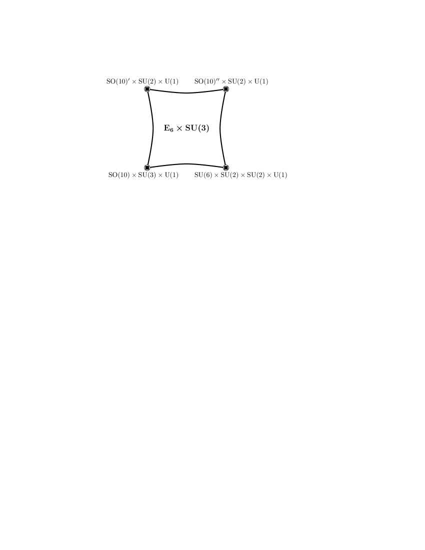
Figure 8: 6D $\mathrm{E}_{6}\times\mathrm{SU}(3)$ orbifold GUT for a large compactification radius of the $\mathrm{SO}(4)$-plane.

The bulk gauge group and the amount of supersymmetry are found via a subset of the invariance conditions (28). Consider a subspace ${\cal S}$ of the 6D compact space with large compactification radii. This subspace is left invariant under the action of some elements of the orbifold space group, i.e. a subset of twists and translations ${\cal G}$. The bulk gauge multiplet in ${\cal S}$ is a subset of the $N=4$ $\mathrm{E}_{8}\times\mathrm{E}_{8}$ gauge multiplet which is invariant under the action of ${\cal G}$, i.e. a subset of conditions (28) restricted to ${\cal G}$.

Consider first the case with two large compact dimensions, for instance those associated with the $\mathrm{SO}(4)$-plane. The $\mathrm{SO}(4)$-plane is invariant under the $\mathbbm{Z}_{3}$ subtwist as well as translations by a lattice vector in the $\mathrm{G}_{2}$ and $\mathrm{SU}(3)$ planes. The latter do not lead to non–trivial projection conditions since there are no Wilson lines in these planes, while the former leads to gauge symmetry and supersymmetry breaking. The light gauge states are described by fields which are constant with respect to $z_{1}$ and $z_{2}$. Invariance under $\mathbbm{Z}_{3}$ requires (see Eq.(28) with $\ell=2$)

$$\Psi_{p,q}(x;z_{3}) = e^{2\pi\mathrm{i}\,(p\cdot V_{3}-q\cdot v_{3})}\Psi_{p,q}\left(x;z_{3}\right)\;.$$ (61)

Gauge multiplets satisfy $q\cdot v_{3}=0$ which has two sets of solutions for $q$ corresponding to $N=2$ supersymmetry. Then the condition $p\cdot V_{3}=0$ breaks $\mathrm{E}_{8}$ to $\mathrm{E}_{6}\times\mathrm{SU}(3)$. At the four fixed points of the $\mathrm{SO}(4)$-plane symmetry is broken further to the four subgroups discussed in Sect. 3. Altogether, we obtain a 6D $\mathrm{E}_{6}\times\mathrm{SU}(3)$ orbifold GUT with the distribution of gauge symmetries in the fundamental region of the orbifold shown in Fig. 8. Similarly, untwisted matter satisfies (61) with $q\cdot v_{3}=\pm 1/3$. We note that all three SM generations live at the origin in Fig. 8.

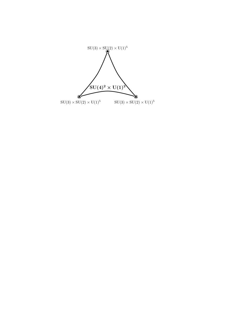
Figure 9: 6D $\mathrm{SU}(4)\times\mathrm{SU}(4)\times\mathrm{U}(1)^{2}$ orbifold GUT for a large compactification radius of the $\mathrm{SU}(3)$-plane.

A similar analysis can be carried out for the $\mathrm{SU}(3)$-plane, which is invariant under the $\mathbbm{Z}_{2}$ subtwist and lattice translations in the $\mathrm{G}_{2}$ and $\mathrm{SO}(4)$ planes. In this case, there are also non–trivial projection conditions due to the Wilson lines,

$$\Psi_{p,q}(x;z_{2}) = e^{2\pi\mathrm{i}\,(p\cdot V_{2}-q\cdot v_{2})}\Psi_{p,q}\left(x;z_{2}\right),$$

$$\Psi_{p,q}(x;z_{2}) = e^{2\pi\mathrm{i}\,p\cdot W_{2}}\Psi_{p,q}\left(x;z_{2}\right)\;,$$

$$\Psi_{p,q}(x;z_{2}) = e^{2\pi\mathrm{i}\,p\cdot W_{2}^{\prime}}\Psi_{p,q}\left(x;z_{2}\right)\;.$$ (62)

This breaks $N=4$ $\mathrm{E}_{8}$ to $N=2$ $\mathrm{SU}(4)\times\mathrm{SU}(4)\times\mathrm{U}(1)^{2}$ in the bulk (Fig. 9). At the fixed points, the symmetry is broken further by the $\mathbbm{Z}_{3}$ twist leaving only the standard model gauge group (up to $\mathrm{U}(1)$’s). Each of the three fixed points carries one generation of the standard model matter.

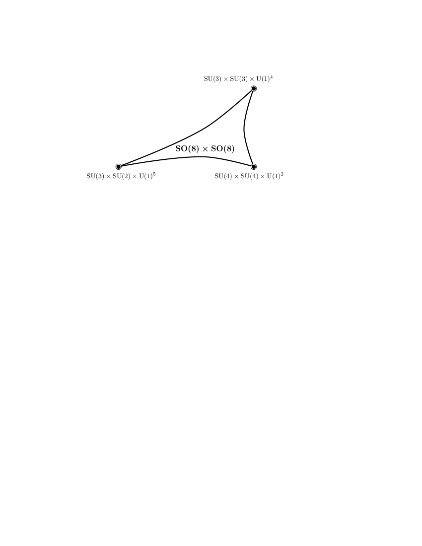
Figure 10: 6D $\mathrm{SO}(8)\times\mathrm{SO}(8)$ orbifold GUT for a large $\mathrm{G}_{2}$-plane compactification radius.

A different picture arises when the $\mathrm{G}_{2}$-plane compactification radius is large. The $\mathrm{G}_{2}$-plane is not invariant under any of the twists, thus there is no projection condition due to twisting. The only non–trivial projection conditions are due to the Wilson lines,

$$\Psi_{p,q}(x;z_{1}) = e^{2\pi\mathrm{i}\,p\cdot W_{2}}\Psi_{p,q}\left(x;z_{1}\right)\;,$$

$$\Psi_{p,q}(x;z_{1}) = e^{2\pi\mathrm{i}\,p\cdot W_{2}^{\prime}}\Psi_{p,q}\left(x;z_{1}\right)\;.$$ (63)

Thus we have $N=4$ supersymmetry and the gauge group is $\mathrm{SO}(8)\times\mathrm{SO}(8)$. Three generations of the standard model are localized at the origin where the $\mathbbm{Z}_{6}$ twist breaks the symmetry to the standard model gauge group (Fig. 10).

	plane
dim.	$\mathrm{G}_{2}$	$\mathrm{SU}(3)$	$\mathrm{SO}(4)$	conditions	SUSY, bulk groups
10				–	$N=4$, $\mathrm{E}_{8}$
9				$p\cdot W_{2}\in\mathbbm{Z}$	$N=4$, $\mathrm{SO}(16)$
9				$p\cdot W_{2}^{\prime}\in\mathbbm{Z}$	$N=4$, $\mathrm{SO}(16)$
8	$\bullet$			–	$N=4$, $\mathrm{E}_{8}$
8		$\bullet$		–	$N=4$, $\mathrm{E}_{8}$
8			$\bullet$	$p\cdot W_{2},\,p\cdot W_{2}^{\prime}\in\mathbbm{Z}$	$N=4$, $\mathrm{SO}(8)\times\mathrm{SO}(8)$
7	$\bullet$			$p\cdot W_{2}\in\mathbbm{Z}$	$N=4$, $\mathrm{SO}(16)$
7	$\bullet$			$p\cdot W_{2}^{\prime}\in\mathbbm{Z}$	$N=4$, $\mathrm{SO}(16)$
7		$\bullet$		$p\cdot W_{2}\in\mathbbm{Z}$	$N=4$, $\mathrm{SO}(16)$
7		$\bullet$		$p\cdot W_{2}^{\prime}\in\mathbbm{Z}$	$N=4$, $\mathrm{SO}(16)$
6	$\bullet$	$\bullet$		$p\cdot 2V_{6}\in\mathbbm{Z}$	$N=2$, $\mathrm{E}_{6}\times\mathrm{SU}(3)$
6	$\bullet$		$\bullet$	$p\cdot 3V_{6},\,p\cdot W_{2},\,p\cdot W_{2}^{\prime}\in\mathbbm{Z}$	$N=2$, $\mathrm{SU}(4)\times\mathrm{SU}(4)$
6		$\bullet$	$\bullet$	$p\cdot W_{2},\,p\cdot W_{2}^{\prime}\in\mathbbm{Z}$	$N=4$, $\mathrm{SO}(8)\times\mathrm{SO}(8)$
5	$\bullet$	$\bullet$		$p\cdot 2V_{6},\,p\cdot W_{2}\in\mathbbm{Z}$	$N=2$, $\mathrm{SU}(6)\times\mathrm{SU}(2)^{2}$
5	$\bullet$	$\bullet$		$p\cdot 2V_{6},\,p\cdot W_{2}^{\prime}\in\mathbbm{Z}$	$N=2$, $\mathrm{SU}(6)\times\mathrm{SU}(2)^{2}$
4	$\bullet$	$\bullet$	$\bullet$	$p\cdot V_{6},\,p\cdot W_{2},\,p\cdot W_{2}^{\prime}\in\mathbbm{Z}$	$\begin{array}[]{l}N=1,\leavevmode\nobreak\ \mathrm{SU}(3)\times\mathrm{SU}(2)\\ \sim G_{\mathrm{SM}}\end{array}$

Table 1: Survey of the various orbifold GUTs in different dimensions. The bullet indicates small compact dimensions. $\mathrm{U}(1)$ factors are omitted.

In principle, there is nothing special about six dimensions, and the same analysis can be carried out for five, seven, eight, nine and ten dimensions. The results are summarized in Table 1. A variety of orbifold GUTs appears, with gauge groups ranging from $\mathrm{E}_{8}$ to $\mathrm{SU}(4)\times\mathrm{SU}(4)\times\mathrm{U}(1)^{2}$. These GUTs represent different points in moduli space. Values of the corresponding T-moduli determine the compactification radii.

It is remarkable that all these GUT models in various dimensions are consistent with gauge coupling unification. This is true even though in some cases $\mathrm{SU}(3)_{c}$ and $\mathrm{SU}(2)_{\mathrm{L}}$ are contained in different simple factors, i.e. $\mathrm{SO}(8)\times\mathrm{SO}(8)$ or $\mathrm{SU}(4)\times\mathrm{SU}(4)$. The beta functions for both $\mathrm{SO}(8)$’s or $\mathrm{SU}(4)$’s are the same. In the former case this is enforced by $N=4$ supersymmetry, while in the latter case the two $\mathrm{SU}(4)$’s have identical bulk matter content, $2\times(\boldsymbol{6,1})+16\times(\boldsymbol{4,1})$ $N=2$ multiplets. In all other cases $\mathrm{SU}(3)_{c}\times\mathrm{SU}(2)_{\mathrm{L}}$ is contained in a simple factor such that unification of the gauge couplings in the bulk is automatic.

On the other hand, different GUTs differ in the value of the gauge coupling at the unification scale, since the power law running depends on the number of extra dimensions and the bulk gauge group. Realization of some of the GUTs may require nonperturbative string coupling [23, 24]. Different models also lead to different Yukawa couplings which depend on the compactification radii. These phenomenological aspects are similar to those of orbifold GUTs [25] and will be discussed elsewhere.

5 Summary

We have presented a $\mathbbm{Z}_{6}$ heterotic orbifold model leading to the standard model spectrum and additional vector–like matter in four dimensions. Standard model generations appear as $\boldsymbol{16}$-plets of $\mathrm{SO}(10)$. They are localized at different fixed points in the compact space with local $\mathrm{SO}(10)\times\mathrm{SU}(3)\times\mathrm{U}(1)$ symmetry.

If some of the compactification radii are significantly larger than the others, we recover various higher–dimensional GUTs as an intermediate step at energies below $M_{S}$. These GUTs have the same 4D massless spectrum and the same ultraviolet completion, but represent different points in moduli space. All of them are consistent with gauge coupling unification, yet differ in other phenomenological aspects.

Acknowledgements. We would like to thank S. Förste, A. Hebecker, T. Kobayashi, H.-P. Nilles, M. Trapletti, P. K. S. Vaudrevange and A. Wingerter for discussions. One of us (M.R.) would like to thank the Aspen Center for Physics for support. This work was partially supported by the EU 6th Framework Program MRTN-CT-2004-503369 “Quest for Unification” and MRTN-CT-2004-005104 “ForcesUniverse”.

References

- [1] H. Georgi, S. L. Glashow, Phys. Rev. Lett. 32 (1974) 438.
-
[2]
H. Georgi, Particles and Fields 1974, ed. C. E. Carlson (AIP, NY, 1975)
p. 575;
H. Fritzsch, P. Minkowski, Ann. of Phys. 93 (1975) 193. - [3] J. C. Pati, A. Salam, Phys. Rev. D 10 (1974) 275.
- [4] S. M. Barr, Phys. Lett. B 112 (1982) 219.
- [5] D. I. Olive, in: Unification of the fundamental particle interactions II (Erice, 1981) eds. J. Ellis and S. Ferrara (Plenum Press, New York, 1983).
- [6] D. J. Gross, J. A. Harvey, E. J. Martinec and R. Rohm, Phys. Rev. Lett. 54, 502 (1985); Nucl. Phys. B 256 (1985) 253.
- [7] P. Candelas, G. T. Horowitz, A. Strominger and E. Witten, Nucl. Phys. B 258 (1985) 46.
- [8] L. J. Dixon, J. A. Harvey, C. Vafa, E. Witten, Nucl. Phys. B 261 (1985) 678; ibid. Nucl. Phys. B 274 (1986) 285.
-
[9]
L. E. Ibáñez, H. P. Nilles, F. Quevedo, Phys. Lett. B 187 (1987) 25;
L. E. Ibáñez, J. E. Kim, H. P. Nilles, F. Quevedo, Phys. Lett. B 191 (1987) 282. -
[10]
Y. Kawamura, Progr. Theor. Phys. 103 (2000) 613; ibid. 105 (2001) 999;
G. Altarelli, F. Feruglio, Phys. Lett. B 511 (2001) 257;
L. J. Hall, Y. Nomura, Phys. Rev. D 64 (2001) 055003;
A. Hebecker, J. March-Russell, Nucl. Phys. B 613 (2001) 3. -
[11]
T. Asaka, W. Buchmüller, L. Covi, Phys. Lett. B 523 (2001) 199;
L. J. Hall, Y. Nomura, T. Okui, D. R. Smith, Phys. Rev. D 65 (2002) 035008. - [12] T. Kobayashi, S. Raby, R.-J. Zhang, Phys. Lett. B 593 (2004) 262.
- [13] S. Förste, H. P. Nilles, P. Vaudrevange, A. Wingerter, Phys. Rev. D 70 (2004) 106008.
- [14] T. Kobayashi, S. Raby, R.-J. Zhang, hep-ph/0409098.
- [15] J. D. Breit, B. A. Ovrut, G. C. Segre, Phys. Lett. B 158 (1985) 33.
- [16] Y. Katsuki, Y. Kawamura, T. Kobayashi, N. Ohtsubo, Y. Ono, K. Tanioka, Nucl. Phys. B 341 (1990) 611.
- [17] K. S. Choi, K. Hwang, J. E. Kim, Nucl. Phys. B 662 (2003) 476.
- [18] A. Hebecker, J. March-Russell, Nucl. Phys. B 625 (2002) 128.
- [19] A. Hebecker, M. Ratz, Nucl. Phys. B 670 (2003) 3.
- [20] L. E. Ibáñez, J. Mas, H. P. Nilles, F. Quevedo, Nucl. Phys. B 301 (1988) 157.
- [21] D. Bailin, A. Love, Phys. Rept. 315 (1999) 285.
- [22] T. Kobayashi, N. Ohtsubo, Phys. Lett. B 245 (1990) 441.
- [23] E. Witten, Nucl. Phys. B 471 (1996) 135.
- [24] A. Hebecker, M. Trapletti, hep-th/0411131.
- [25] T. Asaka, W. Buchmüller, L. Covi, Phys. Lett. B 563 (2003) 209.