MUON PAIR PRODUCTION IN PROTON-ANTIPROTON INTERACTIONS AT INTERMEDIATE ENERGIES.

Abstract

We use PYTHIA event generator to simulate the process of muon pair production in antiproton scattering upon the proton target at the energy of the antiproton equal to $14GeV$, which may be one of the energies for the future PANDA (GSI, Darmstadt) experiment operation.

1 Introduction.

Measurements of lepton pair production in hadron-hadron interactions is of a big interest from the point of view of study of the quark-parton structure of hadrons [1] and [2].

The best example is the discovery of J (also called as J/Psi) charmed meson confirmed later by e+e- experiment tool to get out the information about the parton distribution functions (PDF) in hadrons as it was already shown in a number of high energy experiments [3] and theoretical papers, devoted to the data analysis in the framework of QCD.

In this connection it is worth to mention that up to now there is no good theoretical understanding of the physics of this process. The best example of this situation is the wide use of such a ”theoretical method” of elimination of quite a noticeable discrepancy among the lepton pair production data and the theory predictions (quark-parton model and its QCD extensions) as a simple multiplication of the theory predictions by the so called phenomenological ”K-factors” which values vary in the interval from 1.5 to 2.

Intermediate energy experiments may play an important role as they allow to study the range where the perturbative methods of QCD (pQCD) come into the interplay with a rich physics of bound states. The physics of hadron resonances formation and decays is strongly connected with the confinement problem , i.e. with the QCD dynamics at large distances. Its high precision and detail experimental study would allow to make a serious discrimination between a large variety of non-perturbative approaches and models that are already proposed as well as among those which are under development.

Therefore to define a boundary among perturbative and non-perturbative approaches it may be instructive to make some estimations on kinematical distributions, connected with the $\mu^{+}\mu^{-}$- or $e^{+}e^{-}$- pairs production in the range of future PANDA experiment energies basing upon the well known PYTHIA [4] event generator, which is widely and successfully used in high energy experiments. Such an experience may allow to set the low energy limits for pQCD application as well as it may be also useful for comparison with the predictions of the present (and future) non-perturbative approaches and finding out their difference.

It is worth to mention also that in any case the dominant mechanism of the lepton-anti-lepton pair production would be the same in the most approaches because in this special process $p\bar{p}\rightarrow l\bar{l}+X$ the dominant contribution in any model would come from the same quark pair annihilation amplitude ${q\bar{q}\to l\bar{l}}$. PYTHIA includes this amplitude as well as proper account of relativistic kinematics

To this reason, in present Note we shall simulate in framework of PYTHIA6 the scattering of the anti-protons with the energy of $14GeV$ on the proton target, taken as to be at the rest frame Thus the present simulation would not include the effects connected with the real detector conditions which would be the subject of the following papers.

Thus, the present simulation has the importance as its own because it gives in some sense the ”unbiased distributions” of particles as well as the corresponding quark - parton distributions and allows, in principle, to estimate the size of the corrections needed to reconstruct the original input parton distributions. Let us mention that in what follows we choose MRST4 [5] parameterization of structure functions , which is one from the list of proton parton-distributions set of PYTHIA6.

It should be noted also that the main part of this Note (Sections 1. and 2.) can be easily applied to a case of electron-positron pair production. The main difference of $e^{+}e^{-}$ case with that one of muon pair production is that for $e^{+}e^{-}$ case there would not a big need of discussion of appearance of fake electrons in the same “signal” annihilation event due to negligibly small contribution of fake electrons from pions decays as comparing with their muon decay channel.

2 MUON DISTRIBUTIONS IN $P\bar{P}$ COLLISIONS.

Here we present some distributions of muon physical variables obtained by use of PYTHIA event generator. Its parameters were set to those values that allow fast simulation for the antiproton beam with the energy $E_{beam}$=14 GeV, which corresponds to the center of mass frame energy of $p\bar{p}$ collision $E_{cm}=5.3GeV$.

The muons produced in the corresponding hard QCD $2\rightarrow 2$ subprocess ${q\bar{q}\to\gamma^{*}\to\mu^{+}\mu^{-}}$ would be called in what follows as the ”signal” ones, while those which will appear in event due to meson decays would be called as ”decay” muons.

The simulation was done for a case when both initial state radiation (ISR) and final one (FSR) were switched on (i.e. with the following values of PYTHIA parameters MSTP(61)= MSTP(71)=1). The number of generated events was taken to be 100 000.

The distributions of the signal muons energy $E^{\mu^{+/-}}$ values as well as of the modulus of the transverse momentum $PT^{\mu^{+/-}}$ and of the polar angle $\theta^{\mu^{+/-}}$ (measured from the beam direction) versus the number of generated events are shown (from top to bottom, respectively) in Figure 1 of Section 6, which contains all the Figures. The left column in Figure 1 is for $\mu^{-}$ distributions and the right one for $\mu^{+}$). There is no difference seen between $\mu^{+}$ and the analogous e $\mu^{-}$ distributions in a case when the influence of magnetic field is not considered).

One can see from the top raw of Figure 1 that the energy of muons may vary in the interval $0<E^{\mu}<10GeV$ with a mean value $<E^{\mu}>=2.6$ GeV and a peak at a rather small value $E^{\mu}_{peak}$ =0.5 GeV.

The $PT^{\mu}$ spectrum , see middle raw of Figure 1, has an analogous peak $PT^{\mu}_{peak}=0.5$ GeV/c. After this point both $E^{\mu}$ and $PT^{\mu}$ spectra falls rather steeply but the spectrum of $PT^{\mu}$ is confined in a more narrow interval $0<PT^{\mu}<2$ GeV/c .

The spectrum of events number (Nevent) versus the polar angle ${\theta^{\mu}}$ ( see bottom raw) has a peak at ${\theta^{\mu}}=10^{o}$ and the mean value $<\theta^{\mu}>=27.5^{o}$.

From these plots we see that while the most of signal muons are scattered into the forward direction $\theta^{\mu}<90^{o}$ still there is a small number of them that fly in the backward hemisphere ($\theta^{\mu}>90^{o}$). We shall discuss this point in more details in what follows.

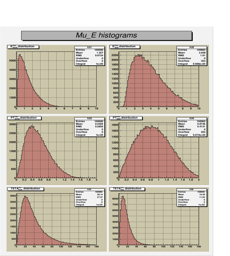
Figure 2: Signal muons distributions for muons with the largest energy (”fast” muons) in the muon pair $E^{\mu}_{fast}$ (left column) and the smaller energy (”slow” muons) $E^{\mu}_{slow}$ (right column). Top raw includes their energies, in middle raw are PT and in bottom raw are $\theta^{\mu}$.

From the view point of the background (the main source for it are the muons from charged pions and other hadrons decays) estimation it is usefull to have the set of plots analogouse to the previouse one, but done separatley for the signal muons having the largest energy ( ”fast” muons) in the muon pair produced in an event , and, correspondently, for those having the smaller energy (”slow” muon). This set of plots for the signal muons are given in Figure 2 of the Appendix, where the left column is for the ”slow” muon distributions and the right one is for ”fast” muons.

We see from Figure 2 that the energy spectrum (top raw) of the fast signal muons grows steeply from the point $E^{\mu}_{fast}=0.5GeV$ (practically $99\%$ of fast muons have $E^{\mu}_{fast}>1GeV$) to the peak at the point $E^{\mu}_{fast}$ = $2.7GeV$ and then vanishes at $E^{\mu}_{fast}$ = $10GeV$.

In contrast to this picture the spectrum of less energetic signal munons (left raw) has a peak at the point $E^{\mu}_{slow}$=0.5 GeV (where the spectrum of fast muons only starts) and it practicaly vanishes at the point, which corresponds to the mean value of the most energetic signal muons, i.e. to $<E^{\mu}_{fast}>$ = 3.9 GeV. Thus, one may say that the spectrum of slow muons in a pair is very different from that of the fast ones.

The difference between the $PT^{\mu}$ spectra (see middle raw of Figure 2) of the fast and slow muons seams not to be so large and it results only in about 340 MeV shift to the left of the peak position as well in the corresponding shift of the end point of slow muons spectrum. Both of these spectra demonstrait that the most of slow as well as of fast muons have $PT^{\mu}>0.2$ GeV.

This similarity of $PT^{\mu}$ spectra of fast and slow muons results (due to a large difference of their energy spectra, i.e. of $P^{\mu}_{z}$ compronent) in a large difference of their polar angle ${\theta^{\mu}}$ distributions (see bottom raw in Figure 2): ${\theta^{\mu}_{slow}}$ spectrum is shifted to the right as comparinring to that one for ${\theta^{\mu}_{fast}}$ and their mean value $<{\theta^{\mu}_{slow}}>$ = $38.2^{o}$ is a more than two times higher than the analogouse mean value for the fast one: $<{\theta^{\mu}_{fast}}>=16.5^{o}$ .

Another and the most important difference that is seen from these angular distributions is that all fast muons fly in forward direction ${\theta^{\mu}_{fast}}<90^{o}$ and their spectrum practically finishes at ${\theta^{\mu}_{fast}}=60^{o}$, while about $17\%$ of slow muons have ${\theta^{\mu}_{slow}}>60^{o}$ and about of $5\%$ of them may scatter into the back hemisphere.

3 SRUCTURE FUNCTIONS:
    u- AND d- QUARK DISTRIBUTIONS.

Up to now we disscussed the results obtained without any other kinematical cuts than those implemented onto internal PYTHIA varaibles and needed to run this generator at as low as possible values of beam energy. In our generation we have restricted the value of the invariant mass of $\mu^{+}\mu^{-}$ signal pair, produced in event. Namely we have taken the last parameter $M_{inv}^{\mu^{+}\mu^{-}}={\hat{s}_{\;min}}$ to be restricted by the inequality $M_{inv}^{\mu^{+}\mu^{-}}>1$ GeV.

The distributions of Bjorken x-variables are shown in Figure 3 for up- and antiup- quarks (top raw) and for down- and antidown- quarks (bottom raw) correspondingly. In what follows we shall refer to these distributions as to the ”unbiased” ones as the influence of different cuts onto muons energy $E^{\mu}_{cut}$ as well as the angle cuts, connected with possible different geometry size of muon muon system would be studied latter. As it can be easialy seen from this plots the obtained distributions do not start from the point x=0, what take place for the used parton distribution parametrizations used in PYTHIA. Such a differnce at low values of x appears due to the mention above cut on the value of muon pair invariant mass.

The number of entries at these plots reflects the valence quark flavour structure of the proton (the analoguse distributions and the number of entries for the antiquarks show the absolute similarity of quark and antiquarks distributions).

4 FAKE MUONS FROM MESON DECAYS.

All what was said above may be to a good approximation applied also to a case of electron-positron pair production in the final state. The most difference of $e^{+}e^{-}$ case with that one of ${\mu^{+}\mu^{-}}$ pair production appears, as it was allready mentioned in the Introduction, when one turns to the problem of background or fake leptons in the same signal lepton pair production process.

Really, the events with a pair of signal muons should contain also some hadrons in the final state. The pions, produced directly or in the decays cascades of other hadrons, may decay in the detector volume and thus serve as a source of background muons that may fake the signal ones produced in the annihilation subprocess.

Figure 4 includes in the left column (as in the Figures 1 and 2) the distributions (from top to bottom) of the number of events versus the energy $E_{PI}$= $E_{\pi}$, the transverse momentum $PT_{PI}$ = ${PT_{\pi}}$ and versus the polar angle $TETA_{PI}$= $\theta_{\pi}$ of produced pions.

The right hand column contains only one plot with the distribution of the total number NPI of charged ${\pi}$-mesons in the signal events. One may see that there is a big number of events ( about$30\%$ ) which do not contain charged pions at all in the final state (they mostly have nucleon pairs in the final state).

This result is very important. Despite the fact that PYTHIA provides a good (at least one of the bests if not the best one) but still a model approximation to the real hadronization effects, it indicates (in the absence of a complete physical and theoretical understanding of parton to hadrons fragmentation processes) that it may happen so that about of one third of events with signal muon pairs may appear practically without additional fake ( or internal background ) decay muons content. That means that muon channel may be quite competitive to the $e^{+}e^{-}$ one. In what follows we shall add more arguments in a favor of this suggestion.

From the same right hand plot we also see that about of $25\%$ of events have only one charged pion in the final state (appearing mostly in ${\Delta}$ resonance decays), and a bit less than $25\%$ of events have two charged pions. It demonstrates also that about of $5\%$ of events have 3 charged pions and there is only about of $1.5\%$ of events with 4 final state charged pions.

Figure 5 includes in the left column, respectively from top to bottom, the energy $E^{\mu}_{dec}$, $PT^{\mu}_{dec}$ and polar angle $\theta^{\mu}_{dec}$ distributions for muons appearing from the discussed above charged ${\pi}$ -meson decays. These distributions follow the analogue spectra of parent pions, presented in Figure 4.

By comparing these plots with those from signal muon pairs shown in Figure 1, one may conclude that the energy mean value of the signal muons $<E^{mu}>$ =2.6 GeV does corresponds to the point in the energy distribution of fake decay muons where the contribution of the decay muons is already low. The same may be said about the PT- distribution of decay muons. The mean value of the PT- distribution of signal muons $PT^{mu}_{signal}=0.7$ GeV (see Figure 1 ) does corresponds to the point where the spectrum of $PT^{mu}_{decay}$ practically vanishes.

The E- and PT- spectra of decay muons are a bit softer than those of “slow” signal ones. They are shifted by 300 MeV (i.e. by $30\%)$ to the left (see their mean values) as comparing with those of signal slow muons. Analogously the fake decay muons polar angle spectrum is shifted also to the left by $30\%$, i.e. by $14^{o}$. Still, due to a big similarity of decay and “slow”signal muons the former may appear as a serious background.

Therefore a reasonable cut upon the muons energy $E^{mu}$ (as well as on the $PT^{mu}$) may lead to an essential reduction of the decay mesons contribution and allow to keep the main part of signal events. Thus a cut $PT^{mu}>0.2$ GeV may allow to get rid of a half of decay mesons at the coast of lost of $8\%$ of signal events . The analogous strict cut $PT^{mu}<0.4$GeV leaves more than $75\%$ of signal muons and less than $15\%$ of decay mesons .

Another way to discriminate the signal “slow” muons from the decay ones is to use the information about the position of the muon production vertex.

The right hand side raw in Figure 5 contains (from top to bottom) the x-, y- and z-(i.e. along the beam direction) components of muon production vertex position, as given by PYTHIA simulation, i.e. in a space free of experimental setup around the interaction point. The distances at these distribution plots are given in millimeters. Thus one may see that the tails of the z-distribution may expand up to 100 meters, while those along x- and y- axis reach 40 meters distance. From this right hand plots it is clearly seen that in a case of mentioned above $66\%$ of signal events that include the decay muons (i.e. addition to the signal muon pair, produced in annihilation subprocess) the size of the detector (i.e., the “decay volume”) may strongly reduce the number of charged ${\pi}$-mesons which potentially may produce muons in the decays because the most of parent pions would interact with the detector components. Therefore one may expect that in the real experimental conditions the situation with the contribution of the additional decay muons may become much easy. The detailed GEANT simulation, which is in our nearest plans, should allow to get more definite predictions about the decay mesons contribution to the background.

5 Conclusion.

The energy, transverse momenta and polar angle (with respect to the beam axis) distributions of muons that may be produced in pairs in $p\bar{p}\rightarrow l\bar{l}+X$ process , i.e. the distributions of signal muons, are presented for a case of the proton target rest frame. These distributions were obtained by use of PYTHIA generator which parameters were adjusted to perform effective generation of physical events in a case of $\bar{p}$ beam energy equal to 14 GeV.

It is shown that those of muons that are the most energetic in a moun pair, i.e. fast muons, predominantly fly in forward direction (with the mean value $<{\theta^{\mu}_{fast}}>=16.5^{o}$) , while those which are less energetic in a pair , i.e. slow muons, fly at larger angles (their mean value is $<{\theta^{\mu}_{slow}}>$ = $38.2^{o}$). It is found that some of slow signal muons may fly in backward hemisphere also. Thus, a good angle coverage by muon system would be very usefull.

The analogous distributions for muons that appear from hadrons decays (mostly from pions), i.e. for decay muons, have shown that decay muons may fake the signal slow muons in the same events and thus, in principle, may be considered to appear as a serious bakground. Nevertheless, the distributions of the number of generated events versus the number of charged pions in lepton pair production event has shown that, fortunatly, more than $30\%$ of signal events do not have charged pions in the final state. On a top of this it seams to be clear from the obtained distribution of the space position of fake decay muon production vertex that a large amount of these muons may be potentialy rejected with the account of the real detector decay volume. We plan as our next step to perform such type of complete GEANT detector simulation with the analysed here events, generated by use of PYHTIA.

The auhtors are very gratefull to G.D.Alexeev for suggestion of this topic for study, the interest to this work and multiple stimulating discussions of the questions concerned.

6 Figures.

Figure 1: Signal muons energy $E^{\mu^{+/-}}$ (top raw), the modulus of the transverse momentum $PT^{\mu^{+/-}}$ (middle raw) and the polar angle $\theta^{\mu^{+/-}}$ (bottom raw) distributions. Left column is for $\mu^{-}$ and right one for $\mu^{+}$.

Figure 3: Top raw shows the distributions of valence up -quarks and anti-quarks, while bottom raw includes the analogous distributions of down-quarks and anti-quarks.

Figure 4: The left column includes the distributions (from top to bottom, respectively) of number of events versus the energy $E_{PI}$=$E_{\pi}$, the transverse momentum $PT_{PI}$= $PT_{\pi}$ and versus the polar angle $TETA_{PI}$= ${\theta_{\pi}}$ of produced pions. The right hand plot shows the distribution of the total number (NPI) of charged ${\pi}$-mesons in the signal events.

Figure 5: The left column includes the distributions (from top to bottom, respectively) of number of events versus the energy $E_{PI}$=$E_{\pi}$, the transverse momentum $PT_{PI}$= $PT_{\pi}$ and versus the polar angle $TETA_{PI}$= ${\theta_{\pi}}$ of produced pions. The right column (from top to bottom) shows the distributions of x-, y- and z- components of decay muon vertex position.

References

- [1] V.A. Matveev, R.M. Muradian, A.N. Tavkhelidze, JINR P2-4543, JINR, Dubna, 1969; SLAC-TRANS-0098, JINR R2-4543, Jun 1969; 27p.
- [2] S.D. Drell, T.M. Yan, SLAC-PUB-0755, Jun 1970, 12p.; Phys.Rev.Lett. 25(1970)316-320, 1970.
- [3] CERN UA1 Collaboration, C. Albajar et al., Phys. Lett., B209 (1988) 397; FNAL E772 Collaboration, P.L. Gaughey at al. Phys. Rev. D50 (1994) 3038;
- [4] T.Sjostrand, Computer Phys. Commun.39 (1986) 347, T.Sjostrand and M.Bengtsson, Computer Phys. Commun.43 (1987 )367.
- [5] A.D. Martin et al., Eur. Phys. J. C4 (1998) 463.
- [6] R. Brun and F. Rademakers, ROOT - An Object Oriented Data Analysis Framework, Proceedings AIHENP’96 Workshop, Lausanne, Sep. 1996, Nucl. Inst. & Meth. in Phys. Res. A389 (1997) 81. See also http://root.cern.ch/.