Heavy quark and quarkonium production
at CERN LEP2: $k_{T}$-factorization versus data

D.V. Skobeltsyn Institute of Nuclear Physics,
M.V. Lomonosov Moscow State University,
119992 Moscow, Russia

Abstract

We present calculations of heavy quark and quarkonium production at CERN LEP2 in the $k_{T}$-factorization QCD approach. Both direct and resolved photon contribution are taken into account. The conservative error analisys is performed. The unintegrated gluon distribution in the photon is taken from the full CCFM evolution equation. The traditional color-singlet mechanism to describe non-perturbative transition of $Q\bar{Q}$-pair into a final quarkonium is used. Our analisys covers polarization properties of heavy quarkonia at moderate and large transverse momenta. We find that the total and differential open charm production cross sections are consistent with the recent experimental data taken by the L3, OPAL and ALEPH collaborations. At the same time the DELPHI data for the inclusive $J/\psi$ production exceed our predictions but experimental uncertainties are too large to claim a significant inconsistency. The bottom production in photon-photon collisions at CERN LEP2 is hard to explain within the $k_{T}$-factorization formalism.

1 Introduction

Heavy quark and quarkonium production in photon-photon collisions at high energies is a subject of the intensive studies from both theoretical and experimental point [1–6]. From the theoretical point, heavy quark in $\gamma\gamma$ collisions can be produced via direct and resolved production mechanisms. In direct events, the two photons couple directly to a heavy quark pair. In resolved events, one photon (”single-resolved”) or both photon (”double-resolved”) fluctuate into a hadronic state and a gluon or a quark of this hadronic fluctuation takes part in the hard interaction. At LEP2 conditions the contribution of the double-resolved events ($gg\to Q\bar{Q}$) is small [7], and charm and bottom quarks are produced mainly via direct ($\gamma\gamma\to Q\bar{Q}$) and single-resolved ($\gamma g\to Q\bar{Q}$) processes. The direct contribution is not dependent on the quark and gluon content in the photon, whereas the single-resolved processes strongly depend on the photon’s gluon density. Therefore detailed knowledge of gluon distributions in the photon is necessary for the theoretical description of such processes at modern (LEP2) and future (TESLA) colliders.

Usually quark and gluon densities are described by the Dokshitzer-Gribov-Lipatov-Altarelli-Parizi (DGLAP) evolution equation [8] where large logarithmic terms proportional to $\ln(\mu^{2})$ are taken into account. The cross sections can be rewritten in terms of process-dependent hard matrix elements convoluted with quark or gluon density functions. In this way the dominant contributions come from diagrams where parton emissions in initial state are strongly ordered in virtuality. This is called collinear factorization, as the strong ordering means that the virtuality of the parton entering the hard scattering matrix elements can be neglected compared to the large scale $\mu^{2}$. However, at the high energies this hard scale is large compare to the $\Lambda_{\rm QCD}$ parameter but on the other hand $\mu^{2}$ is much less than the total energy $\sqrt{s}$ (around 200 GeV for the LEP2 collider). Therefore in such case it was expected that the DGLAP evolution, which is only valid at large $\mu^{2}$, should break down. The situation is classified as ”semihard” [9–12].

It is believed that at assymptotically large energies (or small $x\sim\mu^{2}/s$) the theoretically correct description is given by the Balitsky-Fadin-Kuraev-Lipatov (BFKL) evolution equation [13] because here large terms proportional to $\ln(1/x)$ are taken into account. Just as for DGLAP, in this way it is possible to factorize an observable into a convolution of process-dependent hard matrix elements with universal gluon distributions. But as the virtualities (and transverse momenta) of the propagating gluons are no longer ordered, the matrix elements have to be taken off-shell and the convolution made also over transverse momentum ${\mathbf{k}}_{T}$ with the unintegrated ($k_{T}$-dependent) gluon distribution ${\cal F}(x,{\mathbf{k}}_{T}^{2})$. The unintegrated gluon distribution ${\cal F}(x,{\mathbf{k}}_{T}^{2})$ determines the probability to find a gluon carrying the longitudinal momentum fraction $x$ and the transverse momentum ${\mathbf{k}}_{T}$. This generalized factorization is called $k_{T}$-factorization [10, 11].

The unintegrated gluon distribution is a subject of intensive studies [14]. Various approaches to investigate this quantity have been proposed. One such approach, valid for both small and large $x$, have been developed by Ciafaloni, Catani, Fiorani and Marchesini, and is known as the CCFM model [15]. It introduces angular ordering of emissions to correctly treat gluon coherence effects. In the limit of asymptotic energies, it almost equivalent to BFKL [16–18], but also similar to the DGLAP evolution for large $x$ and high $\mu^{2}$. The resulting unintegrated gluon distribution depends on two scales, the additional scale ${\bar{q}}^{2}$ is a variable related to the maximum angle allowed in the emission and plays the role of the evolution scale $\mu^{2}$ in the collinear parton densities. We will use the following classification scheme [14]: ${\cal F}(x,{\mathbf{k}}_{T}^{2})$ is used for pure BFKL-type unintegrated gluon distributions and ${\cal A}(x,{\mathbf{k}}_{T}^{2},\mu^{2})$ stands for any other type having two scale involved.

The CCFM evolution equation formulated for the proton has been solved numerically or analitically by different ways [19–21]. As it was shown [22–25], unintegrated gluon distribution in the photon ${\cal A}_{\gamma}(x,{\mathbf{k}}_{T}^{2},\mu^{2})$ can be constructed by the similar method as in the proton. But situation is a bit different due to the pointlike component which reflects the splitting of the photon into a quark-antiquark pair. Also in the photon there are no sum rules equivalent to those in the proton case that constrain the quark distributions. However, this difference is not significant because CCFM equation contains only gluon splitting $g\to gg$. For the first time the unintegrated gluon density in the photon was obtained [22] using a simplified solution of the CCFM equation in single loop approximation, when small-$x$ effects can be neglected. It means that the CCFM evolution is reduced to the DGLAP one with the difference that the single loop evolution takes the gluon transverse momentum $k_{T}$ into account. Another simplified solution of the CCFM equation for a photon was proposed [23] using the Kimber-Martin-Ryskin (KMR) prescription [20]. In this way the $\mu^{2}$-dependence in the unintegrated gluon distribution enters only in last step of the evolution, and one-scale evolution equations can be used up to the last step. Both these methods give the similar results [23]. The phenomenological unintegrated gluon density, based on the Golec-Biernat and Wusthoff (GBW) saturation model [24] (extended to the large-$x$ region), was proposed also [23]. Very recently the unintegrated gluon distribution in the photon ${\cal A}_{\gamma}(x,{\mathbf{k}}_{T}^{2},\mu^{2})$ was obtained [25] using the full CCFM evolution equation for the first time. It was shown that the full CCFM evolved effective (integrated over ${\mathbf{k}}_{T}^{2}$) distribution is much higher than the usual DGLAP-based gluon density at $x<10^{-1}$ region.

In the previous studies [23, 25] the unintegrated gluon distributions in a photon (obtained from the single loop as well as full CCFM evolution equation) were applied to the calculation of the open charm and bottom production at LEP2. It was found that total cross section of the charm production is consistent with experimental data. In contrast, the theoretical predictions of the bottom total cross section underestimate data by factor 2 or 3. But we note that all these calculations reveal to the total cross sections of the open charm and bottom production only. In this paper we will study heavy flavored production at LEP2 more detail using the full CCFM-evolved unintegrated gluon density [25]. We will investigate the total and differential heavy quark cross section (namely pseudo-rapidity and transverse momenta distributions of the $D^{*}$-meson) and compare our theoretical results with the recent experimental data taken by the L3, OPAL and ALEPH collaborations at LEP2 [1–5].

Also we will study here the very intriguing problem connected with the inclusive $J/\psi$ meson production at high energies. It is traces back to the early 1990s, when the CDF data on the $J/\psi$ and $\Upsilon$ hadroproduction cross section revealed a more than order of magnitude discrepancy with theoretical expectations. This fact has resulted to intensive theoretical investigations of such processes. In the so-called non-relativistic QCD (NRQCD) [28] there are additional (octet) transition mechanism from $c\bar{c}$ pair to the $J/\psi$ mesons, where $c\bar{c}$ pair is produced in the color octet (CO) state and transforms into final color singlet state (CS) by help soft gluon radiation. The CO model describes well the heavy quarkonium production at Tevatron [29], although there are also some indications that it does not work well. For example, contributions from the octet mechanism to the $J/\psi$ photo- and leptoproduction processes at HERA are not well reproduce [30] experimental data. Also NRQCD is not predict $J/\psi$ polarization properties at HERA and Tevatron [30, 31]. At the same time usual CS model supplemented with $k_{T}$-factorization formalism gives fully correct description of the inclusive $J/\psi$ production at HERA [32] and Tevatron [33] including spin alignement of the quarkonium. The CO contributions within the $k_{T}$-factorization approach also will not contradict experimental data if parameters of the non-perturbative matrix elements will be reduced [33, 34]. But this fact changes hierarchy of these matrix elements which are obtained within the NRQCD.

Recently DELPHI collaboration has presented experimental data [35] on the inclusive $J/\psi$ production in $\gamma\gamma$ collisions at LEP2, which wait to be confronted with different theoretical predictions. The theoretical calculations [36] within the NRQCD formalism agree well with the DELPHI data. In contrast, the collinear DGLAP-based leading order perturbative QCD calculations in the CS model significantly (by order of magnitude) underestimate [36] the data. The aim of this paper, in particular, is to investigate whether the inclusive $J/\psi$ production at LEP2 can be explained in the traditional CS model by using $k_{T}$-factorization and CCFM-based unintegrated gluon density in a photon.

The outline of this paper is following. In Section 2 we present the basic formalism of the $k_{T}$-factorization approach with a brief review of calculation steps. In Section 3 we present the numerical results of our calculations. Finally, in Section 4, we give some conclusion. The compact analytic expressions for the off-shell matrix elements of the all subprocesses under consideration are given in Appendix. These formulas may be useful for the subsequent applications.

2 Cross sections for heavy flavour production

In $\gamma\gamma$ collisions heavy quark and quarkonium can be produced by one of the three mechanisms: a direct production, a single-resolved and a double-resolved production processes. The direct contribution is governed by simple QED amplitudes which is independent on the gluon density in the photon. The double-resolved process gives a much smaller contribution than the direct and single-resolved processes [7] and will not taken into account in this analysis.

Let $p_{\gamma}^{(1)}$ and $p_{\gamma}^{(2)}$ be the momenta of the incoming photons and $p_{1}$ and $p_{2}$ the momenta of the produced quarks. The single-resolved contribution to the $\gamma\gamma\to Q\bar{Q}$ process in the $k_{T}$-factorization approach has the following form:

$$d\sigma_{\rm 1-res}(\gamma\gamma\to Q\bar{Q})=\int{dx\over x}{\cal A}_{\gamma}(x,{\mathbf{k}}_{T}^{2},\mu^{2})d{\mathbf{k}}_{T}^{2}{d\phi\over 2\pi}d\hat{\sigma}(\gamma g^{*}\to Q\bar{Q}),$$

where $\hat{\sigma}(\gamma g^{*}\to Q\bar{Q})$ is the heavy quark production cross section via off-shell gluon having fraction $x$ of a photon longitudinal momentum, non-zero transverse momentum ${\mathbf{k}}_{T}$ (${\mathbf{k}}_{T}^{2}=-k_{T}^{2}\neq 0$) and azimuthal angle $\phi$. The expression (1) can be easily rewritten as

$${d\sigma_{\rm 1-res}(\gamma\gamma\to Q\bar{Q})\over dy_{2}d{\mathbf{p}}_{2T}^{2}}=\int{1\over 16\pi(xs)^{2}(1-\alpha_{2})}{\cal A}_{\gamma}(x,{\mathbf{k}}_{T}^{2},\mu^{2})|\bar{\cal M}|^{2}(\gamma g^{*}\to Q\bar{Q})d{\mathbf{k}}_{T}^{2}{d\phi\over 2\pi}{d\phi_{2}\over 2\pi},$$

where $|\bar{\cal M}|^{2}(\gamma g^{*}\to Q\bar{Q})$ is the off-shell matrix element, $s=(p_{\gamma}^{(1)}+p_{\gamma}^{(2)})^{2}$ is the total c.m. frame energy, $y_{2}$ and $\phi_{2}$ are the rapidity and azimuthal angle of the produced heavy quark having mass $m_{Q}$, $\alpha_{2}=m_{2T}\exp(y_{2})/\sqrt{s}$ and $m_{2T}^{2}=m_{Q}^{2}+{\mathbf{p}}_{2T}^{2}$. To calculate the single-resolved contribution to the inclusive $J/\psi$ production the same formula (2) can be used where off-shell maxtrix element $|\bar{\cal M}|^{2}(\gamma g^{*}\to Q\bar{Q})$ should be replaced by one which corresponds to the $\gamma g^{*}\to J/\psi+g$ production process.

The available experimental data [1–5, 35] refer to heavy quark or quarkonium production in the $e^{+}e^{-}$ collisions also. In order to obtain these total cross sections, the $\gamma\gamma$ cross sections need to be weighted with the photon flux in the electron:

$$d\sigma(e^{+}e^{-}\to e^{+}e^{-}Q\bar{Q}+X)=\int f_{\gamma/e}(x_{1})dx_{1}\int f_{\gamma/e}(x_{2})dx_{2}\,d\sigma(\gamma\gamma\to Q\bar{Q}),$$

where we use the Weizacker-Williams approximation for the bremsstrahlung photon distribution from an electron:

$$f_{\gamma/e}(x)={\alpha\over 2\pi}\left({1+(1-x)^{2}\over x}\ln{Q^{2}_{\rm max}\over Q^{2}_{\rm min}}+2m_{e}^{2}x\left({1\over Q^{2}_{\rm max}}-{1\over Q^{2}_{\rm min}}\right)\right),$$

with $Q^{2}_{\rm min}=m_{e}^{2}x^{2}/(1-x)^{2}$ and $Q^{2}_{\rm max}=Q^{2}_{\rm min}+(E\theta)^{2}(1-x)$. Here $x=E_{\gamma}/E_{e}$, $E=E_{e}={\sqrt{s}}/2$, $s$ is the total energy in the $e^{+}e^{-}$ collision and $\theta\sim 30$ mrad is the angular cut that ensures the photon is quasi-real.

The multidimensional integration in (2) and (3) has been performed by means of the Monte Carlo technique, using the routine VEGAS [37]. The full C$++$ code is available from the authors on request. For reader’s convenience, we collect the analytic expressions for the off-shell matrix elements $|\bar{\cal M}|^{2}(\gamma g^{*}\to Q\bar{Q})$ and $|\bar{\cal M}|^{2}(\gamma g^{*}\to J/\psi g)$ in Appendix, including, in particular, the relevant formulas for helicity zero $J/\psi$ production state.

3 Numerical results

First of all, we can perform integration of the unintegrated gluon distribution ${\cal A}_{\gamma}(x,k_{T}^{2},\mu^{2})$ [25] over gluon transverse momenta ${\mathbf{k}}_{T}^{2}$ to obtain the effective gluon density in the photon:

$$xg_{\gamma}(x,\mu^{2})\sim\int\limits_{0}^{\mu^{2}}{\cal A}_{\gamma}(x,{\mathbf{k}}_{T}^{2},\mu^{2})d{\mathbf{k}}_{T}^{2}.$$

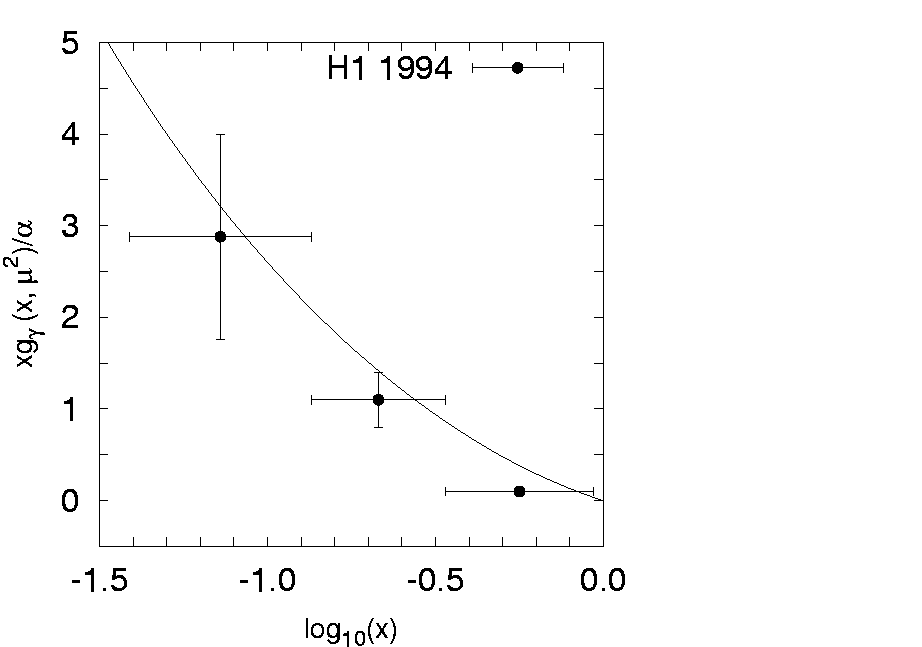
Figure 1: The effective gluon distribution $xg_{\gamma}(x,\mu^{2})$ in the photon as a function of ${\rm log}_{10}x$ at $\mu^{2}=38\,{\rm GeV^{2}}$. The experimental data [38] taken by H1 collaboration from hard dijets production at HERA.

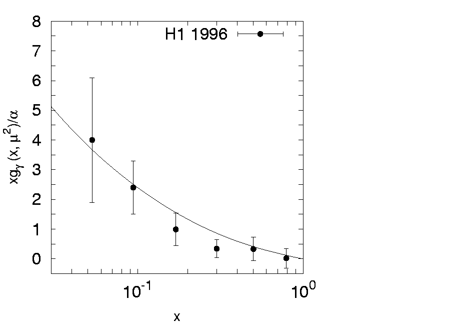
Figure 2: The effective gluon distribution $xg_{\gamma}(x,\mu^{2})$ in the photon as a function of $x$ at $\mu^{2}=74\,{\rm GeV^{2}}$. The experimental data [39] taken by H1 collaboration from hard dijets production at HERA.

The effective density $xg_{\gamma}(x,\mu^{2})$ can be compared with the experimental data [38, 39] taken by H1 collaboration at HERA. As seen in Figures 1 and 2, this gluon distribution agrees well to the existing data extracted from the hard dijet (mean $p_{T}^{2}=38\,{\rm GeV}^{2}$ [38] and $p_{T}^{2}=74\,{\rm GeV}^{2}$ [39]). In contrast, KMR construction of unintegrated gluon density in the photon tends to underestimate the HERA data at $x<10^{-1}$ [23].

Being sure that the full CCFM-evolved unintegrated gluon density ${\cal A}_{\gamma}(x,k_{T}^{2},\mu^{2})$ reproduces well the experimental data for the $xg_{\gamma}(x,\mu^{2})$, we now are in a position to present our numerical results. We describe first our theoretical input and the kinematical conditions. The cross sections for heavy quark and quarkonium production depend on the heavy quark mass and the energy scale $\mu^{2}$. Since there are no free quarks due to confinement effect, their masses cannot be measured directly and should be defined from hadron properties. In our analysis we have examined the following choice: $m_{c}=1.4\pm 0.1$ GeV for charm and $m_{b}=4.75\pm 0.25$ GeV for bottom quark masses. Such variation of the quark masses gives the largest uncertainties in comparison with scale variation and therefore can be used as an estimate of the total theoretical uncertainties. Then, we will apply standard expression $\mu^{2}=m_{Q}^{2}+{\mathbf{p}}_{T}^{2}$ for both renormalization and factorization scales. Here ${\mathbf{p}}_{T}$ is the transverse momentum of the heavy quark in the center-of-mass frame. We use LO formula for the strong coupling constant $\alpha_{s}(\mu^{2})$ with $n_{f}=4$ active quark flavours and $\Lambda_{\rm QCD}=200$ MeV, such that $\alpha_{s}(M_{Z}^{2})=0.1232$. But $\Lambda_{\rm QCD}=340$ MeV [7] was tested also.

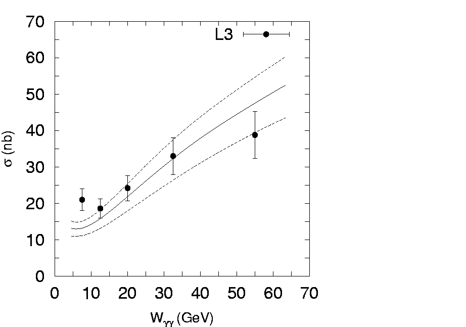
Figure 3: The open charm total cross section $\sigma(\gamma\gamma\to c\bar{c}+X)$ as a function of $W_{\gamma\gamma}$ at $\sqrt{s}=189-202$ GeV. The solid line corresponds to the charm mass $m_{c}=1.4$ GeV, upper and lower dashed lines correspond to the $m_{c}=1.3$ GeV and $m_{c}=1.5$ GeV respectively. The experimental data [2] are taken by the L3 collaboration.

Figure 3 confronts the total cross section $\sigma(\gamma\gamma\to c\bar{c}+X)$ calculated as a function of the photon-photon total energy $W_{\gamma\gamma}$ with experimental data [2] taken by the L3 collaboration in the interval $5<W_{\gamma\gamma}<70$ GeV. Solid line represent the calculations with the charm mass $m_{c}=1.4$ GeV, whereas upper and lower dashed lines correspond to the $m_{c}=1.3$ GeV and $m_{c}=1.5$ GeV respectively. It is clear that $k_{T}$-factorization reproduces well both the energy dependence and the normalization. One can see that sensitivity of the results to the variations of the charm mass is rather large: shifting the mass down to $m_{c}=1.3$ GeV changes the estimated cross section by $15-20$% at $W_{\gamma\gamma}\sim 60$ GeV. But in general all three curves lie within the experimental uncertainties.

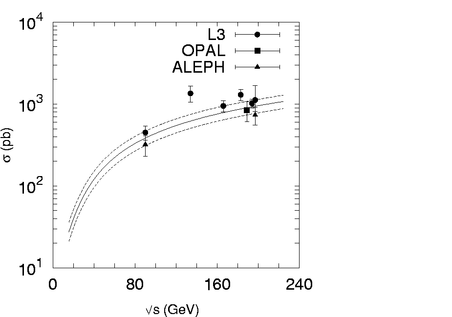
Figure 4: The open charm total cross section $\sigma(e^{+}e^{-}\to e^{+}e^{-}c\bar{c}+X)$ as a function of the $e^{+}e^{-}$ centre-of-mass energy $\sqrt{s}$. All curves are the same as Figure 3. The experimental data are from L3 [1, 3], OPAL [4] and ALEPH [5] collaborations.

Experimental data for the total cross section $\sigma(e^{+}e^{-}\to e^{+}e^{-}c\bar{c}+X)$ come from the three LEP collaborations L3 [1, 3], OPAL [4] and ALEPH [5]. In Figure 4 we show our predictions in comparison with data. All curves here are the same as in Figure 3. One can see that our calculations describe the experimental data well again. The variation of the quark masses $1.3<m_{c}<1.5$ GeV gives the theoretical uncertainties approximately $15$% in absolute normalization.

The available experimental data were obtained for the $D^{*}$ meson production also. Two differential cross section are determined: the first one as a function of the transverse $D^{*}$ momentum $p_{T}$, and the second as a function of pseudo-rapidity $|\eta|$. In our calculation we convert charmed quark into $D^{*}$ meson using the Peterson fragmentation function [41]. The default set for the fragmentation parameter $\epsilon_{c}$ and the fraction $f(c\to D^{*})$ is $\epsilon_{c}=0.06$ and $f(c\to D^{*})=0.26$. Other values for the parameter $\epsilon_{c}$ in the NLO perturbative QCD calculations are often used also, namely $\epsilon_{c}=0.116$ [42] in the massless scheme and $\epsilon_{c}=0.031$ [43] in the massive one. In the case of the massless calculation, this parameter was determined via a NLO fit to LEP1 data on $D^{*}$ production in $e^{+}e^{-}$ annihilation measured by OPAL collaboration [44]. To investigate the sensitivity of the our numerical results to $\epsilon_{c}$ parameter we have repeat our calculations using $\epsilon_{c}=0.031$.

The recent L3 data [3] refer to the kinematic region defined by $1<p_{T}<12$ GeV and $|\eta|<1.4$ with averaged total $e^{+}e^{-}$ energy $\sqrt{s}=193$ GeV ($183<\sqrt{s}<209$ GeV). The OPAL data [4] were obtained in the region $2<p_{T}<12$ GeV, $|n|<1.5$ and averaged over $183<\sqrt{s}<189$ GeV. The more recent ALEPH data [5] refer to the same kinematic region but averaged over $183<\sqrt{s}<209$ GeV. We compare these three data sets with our calculation at $\sqrt{s}=193$ GeV. The different values of $\sqrt{s}$ are not expected to change the cross section more than the corresponding experimental errors. We have checked directly that shifting $\sqrt{s}$ from 189 to 193 GeV increase the calculated cross sections by about one percent only.

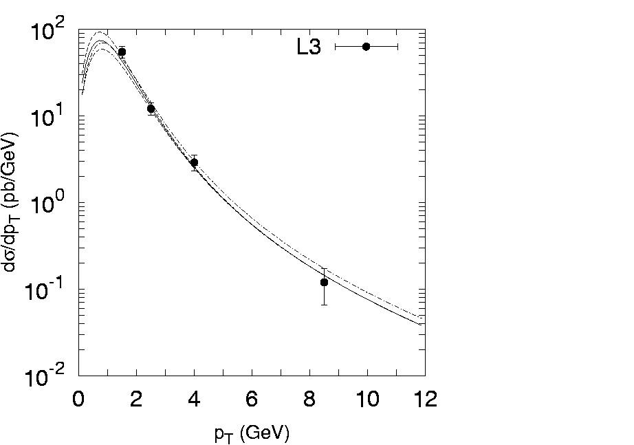
Figure 5: The differential cross section $d\sigma/dp_{T}$ for inclusive $D^{*}$ production at $|\eta|<1.4$. The solid and both dashed curves here are the same as in Figure 3 (calculated with the default value $\epsilon_{c}=0.06$), dash-dotted curve represents results obtained using $\epsilon_{c}=0.031$ and $m_{c}=1.4$ GeV. The experimental data are from L3 [3].

The transverse momenta distributions of the $D^{*}$ meson for different pseudo-rapidity region in comparison to experimental data shown in Figure 5 and 6. The solid and both dashed curves here are the same as in Figure 3 (calculated with the default value $\epsilon_{c}=0.06$), dash-dotted curves represent results obtained using $\epsilon_{c}=0.031$ and $m_{c}=1.4$ GeV. The overall agreement between the our predictions and the data is good although the ALEPH data points in medium and large $p_{T}$ range lie slightly above the theoretical curves. Shifting the $\epsilon_{c}$ default value down to $\epsilon_{c}=0.031$ results to a bit broadening of the $p_{T}$ spectra, which is insufficient to describe the data. The effects come from changing of the charm mass present only at low $p_{T}$: the predicted cross section $d\sigma/dp_{T}$ with $m_{c}=1.3$ GeV is $10-15$% above the one calculated with $m_{c}=1.4$ GeV at $p_{T}\sim 1$ GeV, whereas solid and both dashed theoretical curves practically coincide at medium and large $p_{T}$. The similar effect was found in the NLO perturbative calculation [45], where the difference between the massive and massless approach arises at low $p_{T}$ only.

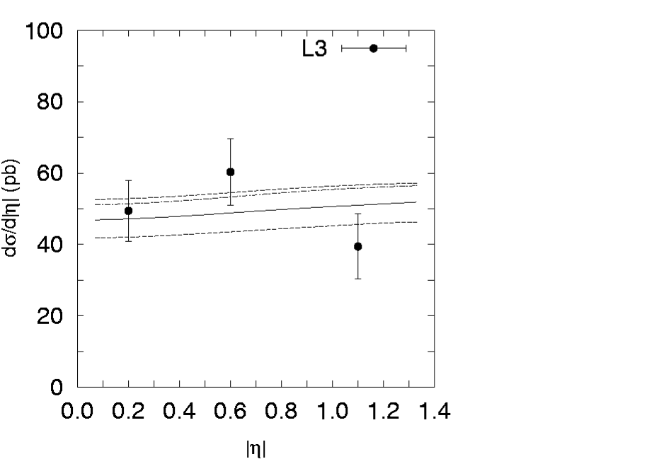
Figure 7: The differential $D^{*}$ cross section $d\sigma/d|\eta|$ for the process $e^{+}e^{-}\to e^{+}e^{-}D^{*}+X$ in the $1<p_{T}<12$ GeV range. All curves here are the same as in Figure 5. The experimental data are from L3 [3].

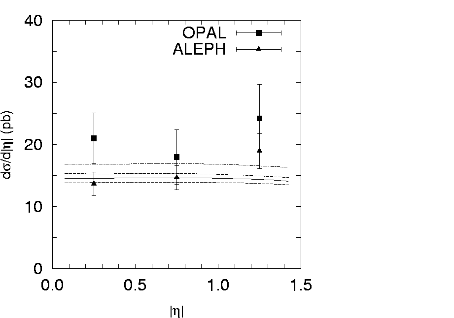
Figure 8: The differential $D^{*}$ cross section $d\sigma/d|\eta|$ for the process $e^{+}e^{-}\to e^{+}e^{-}D^{*}+X$ in the $2<p_{T}<12$ GeV range. All curves here are the same as in Figure 5. The experimental data are from OPAL [4] and ALEPH [5] collaborations.

The $D^{*}$ pseudo-rapidity distributions compared with the experimental data in different $p_{T}$ range are shown in Figure 7 and 8. All curves here are the same as in Figure 5. Our calculations agree well with measured differential cross sections but slightly underestimate the OPAL data. However, setting $\epsilon_{c}=0.031$ increases the absolute normalization of the pseudo-rapidity distribution by approximately $10$%, and agreement with OPAL data becomes better. Again, one can see that the significant mass dependence has place at low transverse momenta only: the difference between the theoretical curves calculated at $2<p_{T}<12$ GeV and plotted in Figure 8 is much smaller than difference between the results presented in Figure 7 obtained at $1<p_{T}<12$ GeV.

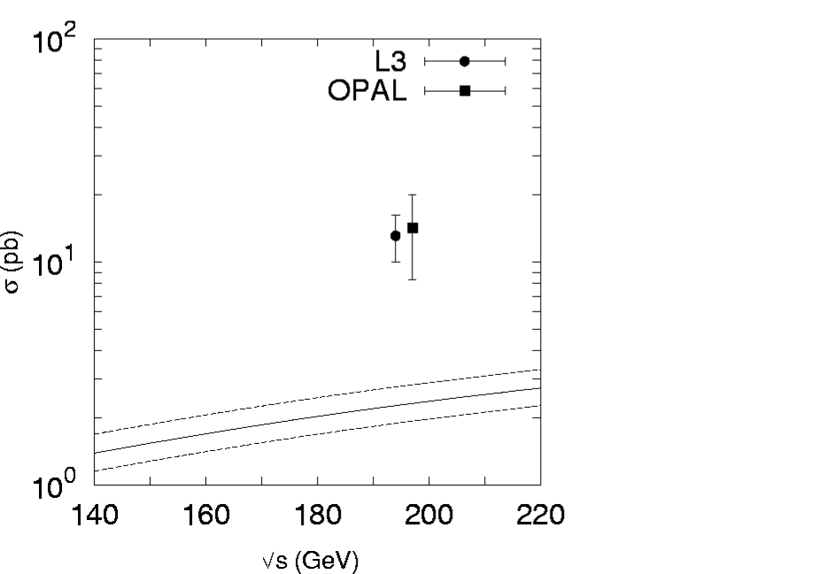
Figure 9: The bottom total cross section $\sigma(e^{+}e^{-}\to e^{+}e^{-}b\bar{b}+X)$ as a function of the $e^{+}e^{-}$ centre-of-mass energy $\sqrt{s}$. The solid line corresponds to the bottom mass $m_{b}=4.75$ GeV, upper and lower dashed lines correspond to the $m_{b}=4.5$ GeV and $m_{b}=5.0$ GeV respectively. The experimental data are from L3 [1] and OPAL [4].

We conclude from Figs. 3 — 8, that our calculations agree well with charm data at LEP2. In contrast with charm case, the open bottom production in $\gamma\gamma$ collisions is clear underestimated by $k_{T}$-factorization. Figure 9 shows our prediction for the open bottom cross section compared to the L3 [1] and OPAL [4] experimental data. Using low but still reasonable $b$-quark mass $m_{b}=4.5$ GeV, we obtain $\sigma(e^{+}e^{-}\to e^{+}e^{-}b\bar{b}+X)=2.94$ pb at $\sqrt{s}=200$ GeV. The very similar value $\sigma=2.7$ pb was obtained [23] within the GBW saturation model adopted for the photon. The Monte Carlo generator CASCADE predicts $\sigma=4.9$ pb [25] where normalization factor $n=1.7$ has been applied for the resolved contributions. The calculation [23] based on the KMR prescription for unintegrated gluon density gives a lower cross section $\sigma=1.9$ pb. At the same time the prediction of the massive NLO perturbative QCD calculation [43] is 3.88 pb for $m_{b}=4.5$ GeV and 2.34 pb for $m_{b}=5.2$ GeV respectively. All these results are significantly (about factor 2 or 3) lower than experimental data.

Such disagreement between theory and data for bottom production at LEP2 is surprising and needs an explanation. It is known that the similar difference between theory and data was claimed for inclusive bottom hadroproduction at Tevatron. Recent analysis indicates that the overall description of the these data can be improved [46] by adopting the non-perturbative fragmentation function of the $b$-quark into $B$ meson: an appropriate treatment of the $b$-quark fragmentation properties considerably reduces the disagreement between measured bottom cross section and the corresponding NLO calculations. It would be interesting to find out whether the similar explanation is also true for the L3 and OPAL experimental data.

After we have studied open heavy quark production at LEP2, we will investigate production of the heavy quarkonum in $\gamma\gamma$ interactions. As it was already mentioned above, non-relativistic QCD gives a good description [36] of the recent DELPHI data [35] on inclusive $J/\psi$ production at LEP2. We will examine whether the DELPHI data can be expained within the CS model using $k_{T}$-factorization approach and CCFM-based unintegrated gluon density in a photon. Again, only direct and single-resolved contributions are taken into account.

Now we change the default set of parameters which were used in the case of open charm calculations. Since we neglect the relative momentum of the $c$-quarks (which form a $J/\psi$ meson) the charm mass should be taken $m_{c}=m_{\psi}/2$. Therefore as default choice in following we will use $m_{c}=1.55$ GeV. On the other hand there are many examples when smaller value $m_{c}=1.4$ GeV in the calculation of $J/\psi$ production is used [30, 32, 36]. In our analysis we will apply this value as extremal choice to investigate the theoretical uncertainties of the calculations.

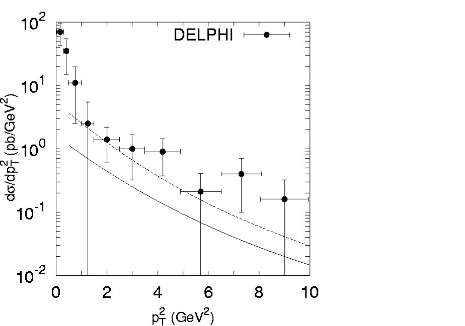
Figure 10: The cross section $d\sigma/dp_{\psi T}^{2}$ of $e^{+}e^{-}\to e^{+}e^{-}J/\psi+X$ measured by DELPHI collaboration [35] at $2<y_{\psi}<2$ as a function of $p_{\psi T}^{2}$ is compared with the $k_{T}$-factorization calculations in the CS model. The solid line corresponds to the $m_{c}=1.55$ GeV and $\Lambda_{\rm QCD}=200$ MeV, dashed line corresponds to the $m_{c}=1.4$ GeV and $\Lambda_{\rm QCD}=340$ MeV.

The DELPHI data [35] refer to the kinematic region defined by $-2<y_{\psi}<2$ with total $e^{+}e^{-}$ energy $\sqrt{s}=197$ GeV, where $y_{\psi}$ is the $J/\psi$ rapidity. However these data were obtained starting from very low transverse momenta $p_{\psi T}^{2}\sim 0.2\,{\rm GeV}^{2}$. We note that $k_{T}$-factorization as well as usual collinear factorization theorem does not work well for such $p_{\psi T}$ values, and our calculations should be compared with experimental data at approximately $p_{\psi T}>1$ GeV only. In Figure 10 we confront our theoretical predictions with the measured differential cross section $d\sigma/dp_{\psi T}^{2}$. Solid line corresponds the default set of parameters and lies below the data by a factor about 2 or 3. This dicrepancy is not catastrofic, because some reasonable variations in $m_{c}$ and $\Lambda_{\rm QCD}$, namely $200<\Lambda_{\rm QCD}<340$ MeV and $1.4<m_{c}<1.55$ GeV, change the estimated cross section by a factor of 3 (dashed line in Figure 9). Thus the visible disagreement is eliminated. However, we do not interpret this as a strong indication of consistency between data and theory, but rather as a concequence of a wide uncertainty band. Better future experimental studies are crucial to determine whether the results of our calculations contradict DELPHI data points.

The main difference between $k_{T}$-factorization and other approaches connects with polarization properties of the final particles because the initial off-shell gluons do promptly manifest in the $J/\psi$ spin alignement [32–34]. Only a very small fraction of $J/\psi$ mesons can be produced in the helicity zero state (longitudinal polarization) by massless bosons. This property is totally determined by the subprocess matrix element structure. The degree of spin alignement can be measured experimentally since the different polarization states of $J/\psi$ result in significantly different angular distributions of the $J/\psi\to\mu^{+}\mu^{-}$ decay leptons:

$${d\Gamma(J/\psi\to\mu^{+}\mu^{-})\over d\cos\theta}\sim 1+\alpha\cos^{2}\theta,$$

where $\alpha=1$ for transverse and $\alpha=-1$ for longitudinal polarizations, respectively. Here $\theta$ is the angle between the lepton and $J/\psi$ directions, measured in $J/\psi$ meson rest frame. We calculate the $p_{T}^{2}$-dependence of the spin alignement parameter as

$$\alpha(p_{\psi T}^{2})={1-3\xi(p_{\psi T}^{2})\over 1+\xi(p_{\psi T}^{2})},$$

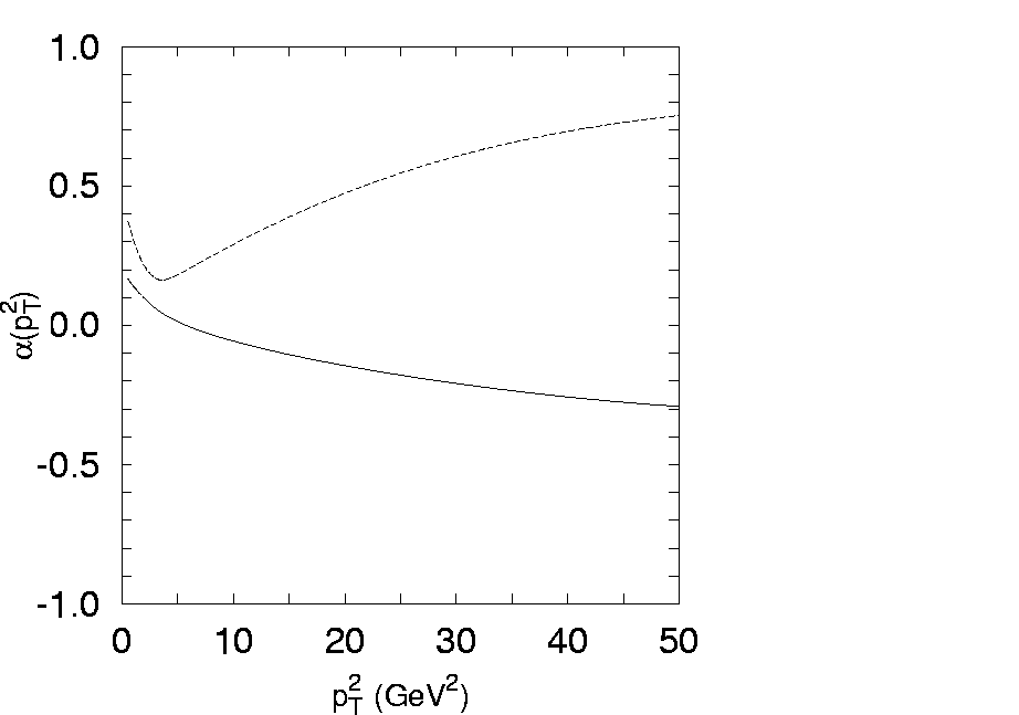
Figure 11: The $p_{\psi T}^{2}$ dependence of the spin alignement parameter $\alpha$ for the inclusive $J/\psi$ production. The solid line corresponds to the $k_{T}$-factorization predictions, dashed line corresponds to the collinear leading order pQCD calculations with the GRV (LO) gluon density in a photon.

with $\xi(p_{\psi T}^{2})$ being the fraction of longitudinally polarized $J/\psi$ mesons. The results of our calculations are shown in Figure 11. Solid line represents the $k_{T}$-factorization predictions and dashed line corresponds to the collinear leading-order pQCD ones with GRV (LO) gluon density [47] in a photon. One can see that fraction of longitudinally polarized mesons increases with $p_{\psi T}^{2}$ within $k_{T}$-factorization approach. This fact is in clear contrast with usual collinear parton model result. The $k_{T}$-factorization calculations made for the inelastic $J/\psi$ production at HERA [32, 34] and Tevatron [33] posses the same behavior of the $\alpha$ parameter, whereas collinear parton model and NRQCD predict the strong transverse polarization at moderate and large $p_{\psi T}^{2}$ range. We point out that our predictions for the $J/\psi$ polarization are stable with respect to variation of the model parameters, such as charmed quark mass and factorization scale. In fact, there is no dependence on the strong coupling constant which is cancels out. At the same time the DELPHI fit [35] gives $\alpha=0.7\pm 1.3$ for $p_{\psi T}^{2}>1\,{\rm GeV^{2}}$, which has, however, huge experimental uncertainties. Since account of the octet contributions does not change predictions of the $k_{T}$-factorization approach for the spin alignement parameter $\alpha$ [33], the future extensive experimental study of such processes will be direct probe of the gluon virtuality.

4 Conclusions

We have investigated a heavy flavour production in photon-photon interactions at high energies within the framework of $k_{T}$-factorization, using unintegrated gluon distribution obtained from the full CCFM evolution equation for a photon. We calculate total and differential cross sections of the open charm and bottom production including $D^{*}$ meson transverse momenta and pseudo-rapidity distributions. Also we have studied inclusive $J/\psi$ production at LEP2 using color-singlet model supplemented with $k_{T}$-factorization.

We take into account both the direct and single-resolved contribution and investigate the sensitivity of the our results to the different parameters, such as heavy quark mass, charm fragmentation and $\Lambda_{\rm QCD}$ parameter. There are, of course, also some uncertainties due to the renormalization and factorization scales. However, these effects would not to be large enough to change the conclusions presented here, and were not taken into account in our analisys.

The results of calculations with default parameter set agree well with open charm production data taken by the L3, OPAL and ALEPH collaborations at LEP2. In contrast, bottom production cross section is clearly underestimated by a factor about 3. A potential explanation of this fact may be, perhaps, connected with the more accurate treatment of the $b$-quark fragmentation function. Our prediction for the inclusive $J/\psi$ production slightly underestimate the DELPHI data. However, a strong inconsistensy cannot be claimed, because of large experimental errors and theoretical uncertainties. Therefore more precise future experiments, espesially polarized quarkonium production, are necessary to know whether our predictions contradict the experimental data.

In conclusion, we point out that at CERN LEP2 collider (as well as at HERA and Tevatron) the difference between predictions of the collinear and $k_{T}$-factorization approaches is clearly visible in polarized heavy quarkonium production. It comes directly from initial gluon off-shellness. The experimental study of such processes should be additional test of non-collinear parton evolution.

5 Acknowledgements

We tnank Hannes Jung for possibility to use the CCFM code for unintegrated gluon distribution in a photon in our calculations. The authors are very grateful also to Sergei Baranov for encouraging interest and helpful discussions. One of us (A.L.) was supported by the INTAS grant YSF’2002 N 399 and by the ”Dynasty” fundation.

6 Appendix

Here we present compact analytic expressions for the off-shell matrix elements which appear in (2). In the following, $\hat{s}$, $\hat{t}$, $\hat{u}$ are usual Mandelstam variables for $2\to 2$ process and $e_{Q}$ is the fractional electric charge of heavy quark $Q$.

We start from photon-gluon fusion $\gamma(q)g^{*}(k)\to Q(p_{1})\bar{Q}(p_{2})$ subprocess, where initial off-shell gluon has non-zero virtuality ${\mathbf{k}}_{T}^{2}$. The corresponding squared matrix element summed over final polarization states and averaged over initial ones read

$$|\bar{\cal M}|^{2}(\gamma g^{*}\to Q\bar{Q})=-{\displaystyle(4\pi)^{2}e_{Q}^{2}\alpha\alpha_{s}\over\displaystyle(\hat{t}-m^{2})^{2}(\hat{u}-m^{2})^{2}}F_{Q\bar{Q}}({\mathbf{k}}_{T}^{2}),$$

where $m$ is the heavy quark mass, and

$$F_{Q\bar{Q}}({\mathbf{k}}_{T}^{2})=6m^{8}-(2{\mathbf{k}}_{T}^{4}+2(\hat{t}+\hat{u}){\mathbf{k}}_{T}^{2}+3{\hat{t}}^{2}+3{\hat{u}}^{2}+14\hat{t}\hat{u})m^{4}+$$

$$(2(\hat{t}+\hat{u}){\mathbf{k}}_{T}^{4}+8\hat{t}\hat{u}{\mathbf{k}}_{T}^{2}+{\hat{t}}^{3}+{\hat{u}}^{3}+7\hat{t}{\hat{u}}^{2}+7{\hat{t}}^{2}\hat{u})m^{2}-$$

$$\hat{t}\hat{u}(2{\mathbf{k}}_{T}^{4}+2(\hat{t}+\hat{u}){\mathbf{k}}_{T}^{2}+{\hat{t}}^{2}+{\hat{u}}^{2}).$$

We note that matrix element of the direct contribution $\gamma\gamma\to Q\bar{Q}$ may be easily obtained from (A.1) and (A.2) in the limit ${\mathbf{k}}_{T}^{2}\to 0$, if we replace normalization factor $(4\pi)^{2}e_{Q}^{2}\alpha\alpha_{s}$ by the $(4\pi)^{2}\alpha^{2}e_{Q}^{4}N_{c}$ (where $N_{c}$ is the number of colors) and average (A.2) over transverse momentum vector ${\mathbf{k}}_{T}$.

Now we are in a position to present our formulas for the $\gamma(q)g^{*}(k)\to J/\psi(p_{\psi})g(p_{g})$ subprocess. In the color-singlet model the production of $J/\psi$ meson is considered as production of a quark-antiquark system in the color-singlet state with orbital momentum $L=1$ and spin momentum $S=1$. The squared off-mass shell matrix element summed over final polarization states and averaged over initial ones can be written as

$$|\bar{\cal M}|^{2}(\gamma g^{*}\to J/\psi g)=-{64e_{Q}^{2}(4\pi)^{3}\alpha\alpha_{s}^{2}|\psi(0)|^{2}\over 3m_{\psi}(\hat{t}-m_{\psi}^{2})^{2}(\hat{u}-m_{\psi}^{2}-{\mathbf{k}}_{T}^{2})^{2}(\hat{t}+\hat{u}+{\mathbf{k}}_{T}^{2})^{2}{\mathbf{k}}_{T}^{2}}F_{\psi}({\mathbf{k}}_{T}^{2}),$$

where $|\psi(0)|^{2}=0.0876\,{\rm GeV}^{3}$ is the $J/\psi$ wave function at the origin, $m_{\psi}$ is the $J/\psi$ meson mass, ${\mathbf{k}}_{T}^{2}$ is the virtuality of the initial gluon, and function $F_{\psi}({\mathbf{k}}_{T}^{2})$ is given by

$$F_{\psi}({\mathbf{k}}_{T}^{2})={\mathbf{k}}_{T}^{2}({\mathbf{k}}_{T}^{6}(m_{\psi}^{2}-\hat{t})(m_{\psi}^{2}-\hat{t}-\hat{u})-m_{\psi}^{2}({\hat{t}}^{2}+\hat{t}\hat{u}+{\hat{u}}^{2}-$$

$$m_{\psi}^{2}(\hat{t}+\hat{u}))^{2}+{\mathbf{k}}_{T}^{4}(3m_{\psi}^{6}+\hat{t}\hat{u}(\hat{t}+\hat{u})-3m_{\psi}^{4}(2\hat{t}+\hat{u})+m_{\psi}^{2}(3{\hat{t}}^{2}+2\hat{t}\hat{u}-{\hat{u}}^{2}))+$$

$${\mathbf{k}}_{T}^{2}(2m_{\psi}^{8}+m_{\psi}^{4}\hat{t}(\hat{t}-\hat{u})-{\hat{t}}^{2}(\hat{t}+\hat{u})^{2}-2m_{\psi}^{6}(2\hat{t}+\hat{u})+m_{\psi}^{2}\hat{t}(2{\hat{t}}^{2}+5\hat{t}\hat{u}+5{\hat{u}}^{2})))+$$

$$2{\mathbf{k}}_{T}^{2}({\mathbf{k}}_{T}^{4}(m_{\psi}^{2}-\hat{t})(m_{\psi}^{2}-\hat{t}-u)+{\mathbf{k}}_{T}^{2}(3m_{\psi}^{6}+\hat{t}(\hat{t}+\hat{u})^{2}-m_{\psi}^{4}(5\hat{t}+3\hat{u})+$$

$$m_{\psi}^{2}({\hat{t}}^{2}+\hat{t}\hat{u}-2{\hat{u}}^{2}))+m_{\psi}^{2}(2m_{\psi}^{6}-m_{\psi}^{4}(3\hat{t}+2\hat{u})+$$

$$\hat{t}({\hat{t}}^{2}+2\hat{t}\hat{u}+3{\hat{u}}^{2})))(-|{\mathbf{p}}_{\psi T}||{\mathbf{k}}_{T}|\cos\phi_{2})+2m_{\psi}^{2}(m_{\psi}^{2}(-m_{\psi}^{2}+\hat{t}+\hat{u})^{2}+$$

$${\mathbf{k}}_{T}^{2}(m_{\psi}^{4}+{\hat{t}}^{2}+2\hat{t}\hat{u}-{\hat{u}}^{2}-2m_{\psi}^{2}(\hat{t}+\hat{u}))){\mathbf{p}}_{\psi T}^{2}{\mathbf{k}}_{T}^{2}\cos^{2}\phi_{2}.$$

Here ${\mathbf{p}}_{\psi T}$ is the $J/\psi$ transverse momentum, $\phi_{2}$ is the azimutal angle of the incoming virtual gluon having virtuality ${\mathbf{k}}_{T}^{2}$. To study polarized $J/\psi$ production we introduce the four-vector of the longitudinal polarization $\epsilon_{\psi,L}^{\mu}$. In the frame where the $z$ axis is oriented along the quarkonium momentum vector, $p_{\psi}^{\mu}=(E_{\psi},0,0,|{\mathbf{p}}_{\psi}|)$, this polarization vector is $\epsilon_{\psi,L}^{\mu}=(|{\mathbf{p}}_{\psi}|,0,0,E_{\psi})/m_{\psi}$. The squared off-shell matrix element read

$$|\bar{\cal M}|_{L}^{2}(\gamma g^{*}\to J/\psi g)={32e_{Q}^{2}(4\pi)^{3}\alpha\alpha_{s}^{2}|\psi(0)|^{2}m_{\psi}\over 3(\hat{t}-m_{\psi}^{2})^{2}(\hat{u}-m_{\psi}^{2}-{\mathbf{k}}_{T}^{2})^{2}(\hat{t}+\hat{u}+{\mathbf{k}}_{T}^{2})^{2}{\mathbf{k}}_{T}^{2}}F_{\psi,L}({\mathbf{k}}_{T}^{2}),$$

where function $F_{\psi,L}({\mathbf{k}}_{T}^{2})$ is defined as

$$F_{\psi,L}({\mathbf{k}}_{T}^{2})=-4{\Delta}_{2}{\Delta}_{3}{\mathbf{k}}_{T}^{4}m_{\psi}^{4}+2{\Delta}_{3}^{2}{\mathbf{k}}_{T}^{4}m_{\psi}^{4}-4{\Delta}_{2}{\Delta}_{3}{\mathbf{k}}_{T}^{2}m_{\psi}^{6}+$$

$$8{\Delta}_{2}{\Delta}_{3}{\mathbf{k}}_{T}^{4}m_{\psi}^{2}\hat{t}-4{\Delta}_{3}^{2}{\mathbf{k}}_{T}^{4}m_{\psi}^{2}\hat{t}+8{\Delta}_{2}{\Delta}_{3}{\mathbf{k}}_{T}^{2}m_{\psi}^{4}\hat{t}+4{\Delta}_{3}^{2}{\mathbf{k}}_{T}^{2}m_{\psi}^{4}\hat{t}-$$

$$4{\Delta}_{2}{\Delta}_{3}{\mathbf{k}}_{T}^{4}{\hat{t}}^{2}+2{\Delta}_{3}^{2}{\mathbf{k}}_{T}^{4}{\hat{t}}^{2}-4{\Delta}_{2}{\Delta}_{3}{\mathbf{k}}_{T}^{2}m_{\psi}^{2}{\hat{t}}^{2}-8{\Delta}_{3}^{2}{\mathbf{k}}_{T}^{2}m_{\psi}^{2}{\hat{t}}^{2}+2{\Delta}_{3}^{2}m_{\psi}^{4}{\hat{t}}^{2}+$$

$$4{\Delta}_{3}^{2}{\mathbf{k}}_{T}^{2}{\hat{t}}^{3}-4{\Delta}_{3}^{2}m_{\psi}^{2}{\hat{t}}^{3}+2{\Delta}_{3}^{2}{\hat{t}}^{4}+4{\Delta}_{2}^{2}{\mathbf{k}}_{T}^{4}m_{\psi}^{2}\hat{u}-$$

$$4{\Delta}_{2}{\Delta}_{3}{\mathbf{k}}_{T}^{4}m_{\psi}^{2}\hat{u}+2{\Delta}_{3}^{2}{\mathbf{k}}_{T}^{4}m_{\psi}^{2}\hat{u}+4{\Delta}_{2}^{2}{\mathbf{k}}_{T}^{2}m_{\psi}^{4}\hat{u}+2{\Delta}_{3}^{2}{\mathbf{k}}_{T}^{2}m_{\psi}^{4}\hat{u}-$$

$$4{\Delta}_{2}^{2}{\mathbf{k}}_{T}^{4}\hat{t}\hat{u}+4{\Delta}_{2}{\Delta}_{3}{\mathbf{k}}_{T}^{4}\hat{t}\hat{u}-2{\Delta}_{3}^{2}{\mathbf{k}}_{T}^{4}\hat{t}\hat{u}-4{\Delta}_{2}^{2}{\mathbf{k}}_{T}^{2}m_{\psi}^{2}\hat{t}\hat{u}-4{\Delta}_{2}{\Delta}_{3}{\mathbf{k}}_{T}^{2}m_{\psi}^{2}\hat{t}\hat{u}-$$

$$4{\Delta}_{3}^{2}{\mathbf{k}}_{T}^{2}m_{\psi}^{2}\hat{t}\hat{u}+2{\Delta}_{3}^{2}m_{\psi}^{4}\hat{t}\hat{u}+4{\Delta}_{2}{\Delta}_{3}{\mathbf{k}}_{T}^{2}{\hat{t}}^{2}\hat{u}+2{\Delta}_{3}^{2}{\mathbf{k}}_{T}^{2}{\hat{t}}^{2}\hat{u}-6{\Delta}_{3}^{2}m_{\psi}^{2}{\hat{t}}^{2}\hat{u}+$$

$$4{\Delta}_{3}^{2}{\hat{t}}^{3}\hat{u}+{\mathbf{k}}_{T}^{6}{\hat{u}}^{2}-4{\Delta}_{2}^{2}{\mathbf{k}}_{T}^{2}m_{\psi}^{2}{\hat{u}}^{2}+4{\Delta}_{2}{\Delta}_{3}{\mathbf{k}}_{T}^{2}m_{\psi}^{2}{\hat{u}}^{2}-2{\Delta}_{3}^{2}{\mathbf{k}}_{T}^{2}m_{\psi}^{2}{\hat{u}}^{2}+{\mathbf{k}}_{T}^{2}m_{\psi}^{4}{\hat{u}}^{2}+$$

$$4{\Delta}_{2}{\Delta}_{3}{\mathbf{k}}_{T}^{2}\hat{t}{\hat{u}}^{2}-2{\Delta}_{3}^{2}{\mathbf{k}}_{T}^{2}\hat{t}{\hat{u}}^{2}-2{\mathbf{k}}_{T}^{4}\hat{t}{\hat{u}}^{2}-2{\Delta}_{3}^{2}m_{\psi}^{2}\hat{t}{\hat{u}}^{2}-2{\mathbf{k}}_{T}^{2}m_{\psi}^{2}\hat{t}{\hat{u}}^{2}+$$

$$2{\Delta}_{3}^{2}{\hat{t}}^{2}{\hat{u}}^{2}+2{\mathbf{k}}_{T}^{2}{\hat{t}}^{2}{\hat{u}}^{2}-2{\mathbf{k}}_{T}^{2}m_{\psi}^{2}{\hat{u}}^{3}+2{\mathbf{k}}_{T}^{2}\hat{t}{\hat{u}}^{3}+{\mathbf{k}}_{T}^{2}{\hat{u}}^{4}+8{\Delta}_{1}^{2}{\mathbf{k}}_{T}^{4}(-m_{\psi}^{2}+\hat{t}+\hat{u})^{2}+$$

$$4{\Delta}_{1}{\mathbf{k}}_{T}^{2}({\Delta}_{2}({\mathbf{k}}_{T}^{4}(2m_{\psi}^{2}-2\hat{t}-\hat{u})+m_{\psi}^{2}(m_{\psi}^{2}-2\hat{t}-\hat{u})\hat{u}+{\mathbf{k}}_{T}^{2}(2m_{\psi}^{4}+{\hat{u}}^{2}-$$

$$2m_{\psi}^{2}(\hat{t}+\hat{u})))+{\Delta}_{3}(-m_{\psi}^{6}+{\mathbf{k}}_{T}^{4}(-m_{\psi}^{2}+\hat{t})+2\hat{t}(\hat{t}+\hat{u})^{2}+$$

$$m_{\psi}^{4}(3\hat{t}+\hat{u})-m_{\psi}^{2}\hat{t}(4\hat{t}+3\hat{u})+{\mathbf{k}}_{T}^{2}(-(m_{\psi}^{2}(2\hat{t}+\hat{u}))+\hat{t}(2\hat{t}+3\hat{u}))))+$$

$$4(-({\Delta}_{2}{\Delta}_{3}({\mathbf{k}}_{T}^{2}+m_{\psi}^{2})(m_{\psi}^{2}-\hat{t})(m_{\psi}^{2}-\hat{t}-\hat{u}))+{\mathbf{k}}_{T}^{2}({\mathbf{k}}_{T}^{2}-\hat{t}){\hat{u}}^{2}+$$

$$4{\Delta}_{1}^{2}{\mathbf{k}}_{T}^{2}(-m_{\psi}^{2}+\hat{t}+\hat{u})^{2}+{\Delta}_{1}(2{\Delta}_{2}{\mathbf{k}}_{T}^{2}(2m_{\psi}^{4}+{\mathbf{k}}_{T}^{2}(2m_{\psi}^{2}-2\hat{t}-\hat{u})-$$

$$2m_{\psi}^{2}(\hat{t}+\hat{u})+\hat{u}(\hat{t}+\hat{u}))-{\Delta}_{3}(m_{\psi}^{6}+{\mathbf{k}}_{T}^{4}(m_{\psi}^{2}-\hat{t}+\hat{u})-$$

$$2\hat{t}(\hat{t}+\hat{u})^{2}-m_{\psi}^{4}(3\hat{t}+2\hat{u})+m_{\psi}^{2}(4{\hat{t}}^{2}+5\hat{t}\hat{u}+{\hat{u}}^{2})+$$

$${\mathbf{k}}_{T}^{2}(-2{\hat{t}}^{2}-t\hat{u}+{\hat{u}}^{2}+m_{\psi}^{2}(2\hat{t}+\hat{u})))))(-|{\mathbf{p}}_{\psi T}||{\mathbf{k}}_{T}|\cos\phi_{2})+$$

$$4(2{\Delta}_{1}{\Delta}_{2}({\mathbf{k}}_{T}^{2}+m_{\psi}^{2})(m_{\psi}^{2}-\hat{t}-\hat{u})+$$

$${\mathbf{k}}_{T}^{2}{\hat{u}}^{2}+2{\Delta}_{1}^{2}(-m_{\psi}^{2}+\hat{t}+\hat{u})^{2}){\mathbf{p}}_{\psi T}^{2}{\mathbf{k}}_{T}^{2}\cos^{2}\phi_{2},$$

and the following notation has been used:

$$\Delta_{1}=(\alpha_{1}+\alpha_{2}){\sqrt{s}\over 2m_{\psi}}\left(\sqrt{{\mathbf{p}}_{\psi T}^{2}+s(\alpha_{1}-\beta_{1})^{2}/4}-{s(\alpha_{1}^{2}-\beta_{1}^{2})\over 4\sqrt{{\mathbf{p}}_{\psi T}^{2}+s(\alpha_{1}-\beta_{1})^{2}/4}}\right),$$

$$\Delta_{2}=(\beta_{1}+\beta_{2}){\sqrt{s}\over 2m_{\psi}}\left(\sqrt{{\mathbf{p}}_{\psi T}^{2}+s(\alpha_{1}-\beta_{1})^{2}/4}+{s(\alpha_{1}^{2}-\beta_{1}^{2})\over 4\sqrt{{\mathbf{p}}_{\psi T}^{2}+s(\alpha_{1}-\beta_{1})^{2}/4}}\right)+\Delta_{3},$$

$$\Delta_{3}=-{\sqrt{s}(\alpha_{1}+\beta_{1})\over 2m_{\psi}\sqrt{{\mathbf{p}}_{\psi T}^{2}+s(\alpha_{1}-\beta_{1})^{2}/4}}|{\mathbf{p}}_{\psi T}||{\mathbf{k}}_{T}|\cos\phi_{2},$$

$$\alpha_{1}=\sqrt{m_{\psi}^{2}+{\mathbf{p}}_{\psi T}^{2}\over s}\exp(y_{\psi}),\quad\beta_{1}=\sqrt{m_{\psi}^{2}+{\mathbf{p}}_{\psi T}^{2}\over s}\exp(-y_{\psi}),$$

$$\alpha_{2}={|{\mathbf{p}}_{gT}|\over\sqrt{s}}\exp(y_{g}),\quad\beta_{2}={|{\mathbf{p}}_{gT}|\over\sqrt{s}}\exp(-y_{g}).$$

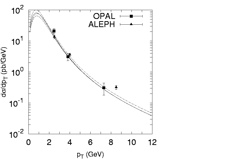
Figure 6: The differential cross section $d\sigma/dp_{T}$ for inclusive $D^{*}$ production at $|\eta|<1.5$. All curves here are the same as in Figure 5. The experimental data are from OPAL [4] and ALEPH [5].

References

- [1] M. Acciari et al. (L3 Collaboration), Phys. Lett. B503, 10 (2001).
- [2] M. Acciari et al. (L3 Collaboration), Phys. Lett. B514, 19 (2001).
- [3] P. Achard et al. (L3 Collaboration), Phys. Lett. B535, 59 (2002).
- [4] G. Abbiendi et al. (OPAL Collaboration), Eur. Phys. J. C16, 579 (2000).
- [5] ALEPH Collaboration, Eur. Phys. J. C28, 437 (2003).
- [6] TESLA Technical Design Report, DESY 2001-11, TESLA Report 2001-23, TESLA-FEL 2001-05.
- [7] M. Drees, M. Krämer, J. Zunft, and P.M. Zerwas, Phys. Lett. B306, 371 (1993).
-
[8]
V.N. Gribov and L.N. Lipatov, Yad. Fiz. 15, 781 (1972);
L.N. Lipatov, Sov. J. Nucl. Phys. 20, 94 (1975);
G. Altarelly and G. Parizi, Nucl. Phys. B126, 298 (1977);
Y.L. Dokshitzer, Sov. Phys. JETP 46, 641 (1977). - [9] V.N. Gribov, E.M. Levin, and M.G. Ryskin, Phys. Rep. 100, 1 (1983).
- [10] E.M. Levin, M.G. Ryskin, Yu.M. Shabelsky, and A.G. Shuvaev, Sov. J. Nucl. Phys. 53, 657 (1991).
- [11] S. Catani, M. Ciafoloni, and F. Hautmann, Nucl. Phys. B366, 135 (1991).
- [12] J.C. Collins and R.K. Ellis, Nucl. Phys. B360, 3 (1991).
-
[13]
E.A. Kuraev, L.N. Lipatov, and V.S. Fadin, Sov. Phys. JETP 44, 443 (1976);
E.A. Kuraev, L.N. Lipatov, and V.S. Fadin, Sov. Phys. JETP 45, 199 (1977);
I.I. Balitsky and L.N. Lipatov, Sov. J. Nucl. Phys. 28, 822 (1978). - [14] B. Andersson et al. (Small- Collaboration), Eur. Phys. J. C25, 77 (2002).
-
[15]
M. Ciafaloni, Nucl. Phys. B296, 49 (1988);
S. Catani, F. Fiorani, and G. Marchesini, Phys. Lett. B234, 339 (1990);
S. Catani, F. Fiorani, and G. Marchesini, Nucl. Phys. B336, 18 (1990);
G. Marchesini, Nucl. Phys. B445, 49 (1995). - [16] J.R. Forshaw and A. Sabio Vera, Phys. Lett. B440, 141 (1998).
- [17] B.R. Webber, Phys. Lett. B444, 81 (1998).
- [18] G.P. Salam, JHEP 03, 009 (1999).
- [19] H. Jung and G.P. Salam, Eur. Phys. J C19, 351 (2001).
- [20] M.A. Kimber, A.D. Martin, and M.G. Ryskin, Phys. Rev. D63, 114027 (2001).
- [21] J. Kwiecinski, Acta Phys. Polon. B33, 1809 (2002).
- [22] A. Gawron and J. Kwiecinski, Acta Phys. Polon. B34, 133 (2003).
- [23] L. Motyka and N. Timneanu, Eur. Phys. J. C27, 73 (2003).
-
[24]
K. Golec-Biernat and M. Wüsthoff, Phys. Rev. D59, 014017 (1999);
K. Golec-Biernat and M. Wüsthoff, Phys. Rev. D60, 114023 (1999). - [25] M. Hansson, H. Jung, and L. Jönsson, hep-ph/0402019.
- [26] A.V. Lipatov and N.P. Zotov, hep-ph/0304181.
- [27] J. Blümlein, DESY 95-121; DESY 95-125.
- [28] G.T. Bodwin, E. Braaten, and G.P. Lepage, Phys. Rev. D51, 1125 (1995); D55, 5853 (1997).
-
[29]
E. Braaten and S. Fleming, Phys. Rev. Lett. 74, 3327 (1995);
E. Braaten and T.C. Yuan, Phys. Rev. D52, 6627 (1995);
P. Cho and A.K. Leibovich, Phys. Rev. D53, 150 (1996); D53, 6203 (1996). -
[30]
M. Cacciari and M. Kramër, Phys. Rev. Lett. 76, 4128 (1996);
P. Ko, J. Lee, and H.-S. Song, Phys. Rev. D54, 4312 (1996);
M. Beneke, M. Kramër, and M. Vänttinen, Phys. Rev. D57, 4258 (1998). -
[31]
M. Beneke and M. Kramër, Phys. Rev. 55, 5269 (1997);
A.K. Leibovich, Phys. Rev. D56, 4412 (1997);
E. Braaten, B.A. Kniehl, and J. Lee, Phys. Rev. D62, 094005 (2000). -
[32]
A.V. Lipatov and N.P. Zotov, Eur. Phys. J. C27, 87 (2003);
A.V. Lipatov and N.P. Zotov, Yad. Fiz. 67, 846 (2004). - [33] S.P. Baranov, Phys. Rev. D66, 114003 (2002).
-
[34]
S.P. Baranov, Phys. Lett. B428, 377 (1998);
S.P. Baranov and N.P. Zotov, J. Phys. G29, 1395 (2003). - [35] J. Abdallah et al. (DELPHI Collaboration), Phys. Lett. B565, 76 (2003).
- [36] M. Klasen, B.A. Kniehl, L.N. Mihaila, and M. Steinhauser, Phys. Rev. Lett. 89, 032001 (2002).
- [37] G.P. Lepage, J. Comput. Phys. 27, 192 (1978).
- [38] C. Adloff et al. (H1 Collaboration), Eur. Phys. J. C10, 363 (1999).
- [39] C. Adloff et al. (H1 Collaboration), Phys. Lett. B483, 36 (2000).
- [40] H. Jung, Comput. Phys. Comm. 143, 100 (2002).
- [41] C. Peterson, D. Schlatter, I. Schmitt, and P. Zervas, Phys. Rev. D27, 105 (1983).
- [42] S. Frixione, M. Krämer, and E. Laenen, Nucl. Phys. B571, 169 (2000).
- [43] J. Binnewies, B.A. Kniehl, and G. Krämer, Phys. Rev. D53, 6110 (1996); D58, 014014 (1998).
- [44] K. Ackerstaff et al. (OPAL Collaboration), Eur. Phys. J. C1, 439 (1998).
- [45] G. Krämer and H. Spiesberger, Eur. Phys. J. C22, 289 (2001).
-
[46]
M. Cacciari and P. Nason, Phys. Rev. Lett. 89, 122003 (2002);
M. Cacciari, S. Frixione, M.L. Mangano, P. Nason, and G. Ridolfi, JHEP 0407, 033 (2004). - [47] M. Glück, E. Reya, and A. Vogt, Z. Phys. C67, 433 (1995).