WHAT BLACK HOLES CAN TEACH US

Abstract

Black holes merge together different field of physics. From General Relativity over thermodynamics and quantum field theory, they do now also reach into the regime of particle and collider physics. In the presence of additional compactified dimensions, it would be possible to produce tiny black holes at future colliders. We would be able to test Planck scale physics and the onset of quantum gravity. The understanding of black hole physics is a key knowledge to the phenomenology of these new effects beyond the Standard Model.

This article gives a brief introduction into the main issues and is addressed to a non-expert audience.

1 Introduction

Gravity is different. Physicists have successfully described three of the known particle interactions in the Standard Model of particle physics. The electromagnetic interaction, which governs the motion of electrically charged particles, the weak interaction, which is e.g. responsible for the beta decay, and the strong interaction, which bounds together the nuclei that we are made of. These three forces can be described as quantum field theories whose mathematical traps and physical details are thought to be well known; if not understood then they are at least familiar.

Only gravity refuses to fit in the common treatment. That gravity is somewhat special can be experienced in daily life. It is the only long range interaction and thus governs the dynamics of macroscopic objects, such as apples, planets or galaxies. Gravity is by far weaker than the other interactions. The strength of the electromagnetic force between two electrons is $\approx 10^{40}$ larger than the gravitational one! The only reason why we do observe it at all is that the gravitational attraction can not be neutralized. The charge of gravity, the mass, is always positive. But for all purposes of particle physics at small distances, the other interactions dominate and gravity can, and is, safely neglected.

This article is organized as follows. In the next section we will introduce the Planck scale and motivate its importance. Section three then reviews briefly some of the main features of black holes, including the evaporation characteristics. In Section four we will summarize the effective models with extra space time dimensions and examine some of the predicted observables. Section five then deals with black holes in these models with extra dimensions, the possibility of their production in the laboratory, their properties and observables. Section six investigates the formation of stable black hole remnants. In Section 7 we connect black hole physic to the issue of a minimal length scale. Section 8 is dedicated to the recurring question whether the earth produced black holes are dangerous. We conclude with a brief summary in Section 9.

Unless otherwise indicated, we assume natural units $\hbar=c=1$ which leads to $m_{\rm p}=1/l_{\rm p}$. The metric has signature $(-1,1,1,...)$.

2 The Planck Scale

For the description of particle physics in the laboratory, interactions of the Standard Model dominate and gravity can be safely neglected. But things will change dramatically if we go to extreme regimes. Let us consider a test particle that is accelerated to a very high energy $E$. As we know from quantum mechanics, such a particle can, and must be, associated with a Compton wave length $\lambda=1/E$. On the other hand, Einstein’s Theory of General Relativity tells us that every kind of energy will cause space time to curve. This is described by Einstein’s Field Equations:

$$R_{\mu\nu}-\frac{1}{2}g_{\mu\nu}R=-8\pi\frac{1}{m_{\rm p}^{2}}T_{\mu\nu}\quad.$$ (1)

The sources of gravity are everything which carries energy and momentum. These quantities are described in the energy momentum tensor $T_{\mu\nu}$ on the right hand side. The sources cause a curvature of spacetime which is described by the metric $g_{\mu\nu}$, and some of its second derivatives in the curvature tensor $R$. This in turn will then modify the motion of the sources in the very space time, giving a self consistent time evolution of the system.

The equation of motions for a pointlike particle is the Geodesic equation:

$$\frac{{\mathrm{d}}^{2}x^{\mu}}{{\mathrm{d}}\tau^{2}}+\Gamma^{\mu}_{\alpha\beta}\frac{{\mathrm{d}}x^{\alpha}}{{\mathrm{d}}\tau}\frac{{\mathrm{d}}x^{\beta}}{{\mathrm{d}}\tau}=0\quad,$$ (2)

where the Christoffel-symbols $\Gamma$ are defined in Eq. (58) and $\tau$ is the eigen time.

The metric of space time has mass dimension $0$. Since the curvature is a second derivative, is has mass dimension $2$. But the energy momentum tensor in three spacelike dimensions has dimension $1+3$. To get the dimensions right in Eq.(1), we thus have to introduce a mass scale $m_{\rm p}$ with a power of $2$, the so called Planck scale.

The exterior metric of an arbitrary spherical symmetric mass distribution with mass $M$ is described by the Schwarzschild solution [1]:

$${\mathrm{d}}s^{2}=g_{\mu\nu}{\rm d}x^{\mu}{\rm d}x^{\nu}=-\gamma(r){\mathrm{d}}t^{2}+\gamma(r)^{-1}{\mathrm{d}}r^{2}+r^{2}{\mathrm{d}}\Omega^{2}\quad,$$ (3)

where

$$\gamma(r)=1-\frac{1}{m_{\rm p}^{2}}\frac{2M}{r}\quad,$$ (4)

and ${\mathrm{d}}\Omega$ is the surface element of the 3-dimensional unit sphere.

To identify the constant $m_{\rm p}$, we take the limit to the familiar Newtonian potential by considering a slow motion in a static gravitational field. Here, slow means slow relative to the speed of light in which case the eigen time is almost identical to the coordinate time, ${\rm d}t/{\rm d}\tau\approx 1$, and for the spatial coordinates $i=1,2,3$ it is ${\rm d}x^{i}/{\rm d}\tau\approx 0$ in Eq.(2). This yields the approximation

$$\frac{{\mathrm{d}}^{2}x^{i}}{{\mathrm{d}}\tau^{2}} \approx \frac{{\mathrm{d}}^{2}x^{i}}{{\mathrm{d}}t^{2}}\approx-\Gamma^{i}_{tt}\left(\frac{{\mathrm{d}}t}{{\mathrm{d}}\tau}\right)^{2}\approx-\Gamma^{i}_{tt}=g^{ij}\Gamma_{jtt}\quad.$$ (5)

Using the definition of the Christoffel-symbols Eq.(58) and taking into account the time independence of the gravitational field, $\partial_{t}g_{\mu\nu}\approx 0$, we obtain

$$\frac{{\mathrm{d}}^{2}x^{i}}{{\mathrm{d}}t^{2}}\approx-\frac{1}{2}g_{tt,i}\;\;.$$ (6)

Inserting Eq. (4) then yields

$$\frac{{\mathrm{d}}^{2}x^{i}}{{\mathrm{d}}t^{2}}\approx-\frac{M}{m_{\rm p}^{2}}\frac{1}{r^{2}}\quad,$$ (7)

and we can identify the quantity $\gamma$ with the Newtonian Potential $\phi$ by

$$\gamma(r)=1-2\phi(r)\quad.$$ (8)

So, it is $m_{\rm p}^{2}=1/G$, the inverse of the Newtonian constant, and the Planck mass turns out to be $\approx 10^{16}$ TeV. Compared to the typical mass scales of the strong and electroweak interactions, which are $\approx 100$ GeV, this is a huge value and reflects the fact that gravity is much weaker. This large gap between the mass scales of the Standard Model and gravity is also called the hierarchy problem.

Let us now come back to our test particle with a very high energy. Looking at Eq.(4), we see that the energy $E$ inside a space time volume with side length given by the Coulomb wave length $\lambda$, will cause a perturbation of the metric which is of order $E^{2}/m_{\rm p}^{2}$. Since flat space is described by $\gamma=1$, we can therefore draw the very important conclusion that a particle with an energy close to the Planck mass will cause a non negligible perturbation of space time on length scales comparable to its own Compton wavelength. Such a particle then should be subject to the yet unknown theory of quantum gravity. Physics at the Planck scale thus represents a future challenge, located between particle physics and General Relativity.

3 Black Holes

Black holes are an immediate consequence of the Schwarzschild solution Eq.(3). As we see, the metric component $g_{tt}=\gamma(r)$ has a zero at the radius $R_{H}=2M/m_{\rm p}^{2}$, the so called Schwarzschild radius. For usual stellar objects like our sun is, this radius lies well inside the mass distributions where the exterior solution does no longer apply. However, if the mass is so densely packed that it has a radius smaller than $R_{H}$, we will be confronted with the consequences of $g_{tt}$ having a zero.

The effect is described most effective by looking at the redshift of a photon. This photon is send out with frequency $\nu_{0}$ by an observer at radius $r_{0}$ and is received at a radius $r_{1}>r_{0}$ with frequency $\nu_{1}$. To exclude effects due to Doppler shift, we assume both, sender and receiver, are in rest. Frequencies count oscillations per time, so their relation is inverse to the relation of the eigen time intervals at both locations

$$\frac{{\rm d}\tau_{1}}{{\rm d}\tau_{0}}=\frac{\nu_{0}}{\nu_{1}}\;\;.$$ (9)

Since both observers are in rest, it is ${\mathrm{d}}r^{2}={\mathrm{d}}\theta^{2}={\mathrm{d}}\phi^{2}=0$ on their world lines. The relation between the eigen times, ${\rm d}\tau_{0/1}^{2}=-{\rm d}s_{0/1}^{2}$, and the coordinate times is given by the metric in Eq.(3)

$${\mathrm{d}}\tau_{0}^{2}=\gamma(r_{0}){\mathrm{d}}t^{2}\quad,\quad{\mathrm{d}}\tau_{1}^{2}=\gamma(r_{1}){\mathrm{d}}t^{2}\quad.$$ (10)

By taking the square root and inserting the eigen time intervals into Eq.(9) we find that the photon will be received at the location $r_{1}$ with a frequency

$$\nu_{1}=\nu_{0}\frac{\sqrt{\gamma(r_{1})}}{\sqrt{\gamma(r_{0})}}\quad.$$ (11)

This redshift goes to infinity for $r_{0}\to R_{H}$, $\gamma(r_{0})\to 0$. In this case, when the sender is close to the Schwarzschild radius, the photon can not be sent out, no matter how high its initial energy is. Thus, no information will ever reach the observer at $r_{1}$. More generally speaking, it turns out that at $R_{H}$ the space time has a trapped surface. What holds for the photon must also hold for slower moving objects. Nothing can ever escape from the region inside the Schwarzschild radius. The object is completely black: a black hole. The radius $R_{H}$ is also called the event horizon.

figure

The last greetings from the astronaut who crosses the Schwarzschild radius. The left strip shows the pictures he sends out and the right strip shows the pictures that are received by an observer who is far away from the horizon.

It is noteworthy at this point that the existence of a horizon, weird at it might seem, is not troublesome in any regard. Even though the Schwarzschild metric in the above given form Eq.(3) has a pole in the $g_{rr}$ component at $R_{H}$, this pole is not a physical one, meaning it can be removed by a suitable coordinate transformation. All of the curvature components are perfectly well behaved at the horizon.

The dependence of the eigen time intervals on the location of the observer can be illustrated by examining the information that is sent out by an infalling observer. Though the above derived expression is not appropriate in this case (the observer is not located at a fixed radius), the result is qualitatively the same, see e.g. [2].

The observer who approaches the horizon sends out information in time intervals which are of equal length in his eigen time as depicted in Figure 3, left. These pictures are received by an observer located at an arbitrary large radius. Here, space time is flat and the coordinate time is identical to the eigen time.

The pictures which are received by the observer far away from the horizon are shown in Figure 3, right. When looking at the last greetings from the infalling observer, the receiver will notice that the time intervals the infalling observer claimed to have equal length become longer and longer. Also, the wave lengths of the photons become longer and the colors are red shifted as derived above. But in addition, it seems to the receiver that every motion of his infalling friend becomes slow motion until it eventually freezes when the sender crosses the event horizon.

This of course does not only apply for infalling observers but also for the collapsing matter. For this reason, black holes have also been termed ’frozen stars’.

What can not be removed is the singularity at $r=0$, which turns out to be a point with infinite curvature. Infinities in physics usually signal that we have missed some essential point in our mathematical treatment and, once again, indicate that the extreme regions of gravity are poorly understood.

3.1 Radiation of Black Holes

In 1975, Hawking published his computation about the radiation of black holes [3]. He showed that a black hole can emit particles if one takes into account the effects of quantum gravity in curved space time. Since the not so black hole of mass $M$ is quasi-static (it is ’frozen’), the spectrum is a thermal spectrum and can be related to a temperature

$$T=\frac{\kappa}{2\pi}\quad,\quad\mbox{with}\quad\kappa=\frac{1}{2}\partial_{r}\gamma(r)\big{|}_{r=R_{H}}\quad,$$ (12)

where $\kappa$ is the surface gravity of the black hole. If one inserts all constants one finds this temperature to be extremely small

$$T=\frac{1}{8\pi}\frac{c^{2}m_{\rm p}^{2}}{k_{B}}\frac{1}{M}\approx 10^{-6}\frac{M_{\odot}}{M}[\mathrm{K}]\quad.$$ (13)

Here, $M_{\odot}\approx 10^{54}$ TeV is the mass of the sun.

The smaller the mass of the black hole, the higher is its temperature. It is remarkable that this formula for the first time connects all fundamental constants and joins gravitation, quantum field theory and thermodynamics.

figure

[h]

Particle creation at the horizon.

To understand this so called Hawking effect, we will use a simple analogy. The effect is similar to the particle production out of vacuum in quantum electrodynamics. In both cases, a strong external field is present. The vacuum is thought to be filled with virtual pairs of particles. In a background field strong enough, the virtual pairs can be ripped apart and form a real pair. The energy for this pair creation is provided by the background field. Figure 3.1 shows a schematic picture of this process. These analogies of course should not be put too far and can not replace a proper calculation. But they provide us with a phenomenological understanding of the effect.

One should be aware of two crucial differences to the electromagnetic case. One essential difference is that, in contrast to the electromagnetic case, in the gravitational case not the actual strength of the field is responsible for the pairs becoming real but its tidal forces are. This is due to the fact that the ’charges’ of gravity are always positive. The second weak point of this analogy is that the energy of the gravitational field is not a well defined quantity. Since gravity is build on the fact that a local observer can not distinguish between gravity and acceleration, this energy is a coordinate dependent quantity and can e.g. be defined in the asymptotically flat coordinate system. In this system, the energy of the infalling particle is apparently negative (this is due to $g_{tt}$ being negative, see Eq. (3)). The black hole therefore looses mass when one of the particles escapes and the other one falls in, as we would have expected.

This picture will be sufficient for our purposes. More details on the calculation can be found e.g. in [4, 5, 6].

The thermodynamic of black holes [2, 4] can be put even further and reveals amazing parallels by relating geometrical quantities of the hole to thermodynamic variables. The most important of this quantities is the entropy $S$.

We know from the standard thermodynamics that the integrating factor of the entropy is the inverse of the temperature. By identifying the total energy of the system with the mass of the black hole we find

$$\frac{\partial S}{\partial M}=\frac{1}{T}\quad.$$ (14)

After inserting Eq. (12)

$$\frac{\partial S}{\partial M}=8\pi\frac{M}{m_{\rm p}^{2}}$$ (15)

and integrating we obtain

$$S(M) = 4\pi\left(\frac{M}{m_{\rm p}}\right)^{2}+{\mbox{const.}}$$ (16)

$$= \frac{m_{\rm p}^{2}}{4}{\cal{A}}+{\mbox{const.}}\quad,$$

where ${\cal{A}}=4\pi R_{H}^{2}$ is the surface of the black hole. The additive constant is not relevant for our further treatment and we will set it to zero.

The black hole looses mass through the evaporation process. Eq. (13) then states that the temperature will be increased by this, resulting in an even faster mass loss. Using the above results, we can estimate the lifetime of the black hole under the assumption that it is a slow process. With all constants, the energy density of the radiation is then given by Stefan-Boltzmann’s law

$$\varepsilon=\frac{\pi^{2}}{30\hbar^{3}c^{2}}(k_{B}T_{S})^{4}\;\;.$$ (17)

The variation of the mass of the black hole itself is then

$$\frac{{\mathrm{d}}M}{{\mathrm{d}}t}\approx-\varepsilon{\cal A}=-\frac{1}{15\pi 8^{3}}\frac{c^{4}\hbar}{G^{2}}\frac{1}{M_{0}^{2}}\quad,$$ (18)

where $M_{0}$ is the initial mass of the black hole under investigation. By integration over $t$ we find for the lifetime

$$\tau\approx{15\pi 8^{3}}\frac{G^{2}}{c^{4}\hbar}M_{0}^{3}\approx 10^{59}\left(\frac{M_{0}}{M_{\odot}}\right)^{3}\mathrm{Gyr}\quad,$$ (19)

after which the mass $M$ is reduced to 0.

To get a grip on this quantity for astrophysical objects, let us insert some numbers. For black holes caused by collapse of usual astrophysical objects, it is $M_{0}>10^{15}$ g and $\tau$ exceeds the age of the universe ($\approx 10^{10}$ years). For super massive black holes, caused by secondary collapse of whole star clusters with typical masses of $M_{0}\geq 10^{27}$ g, the temperature is even below the 3K cosmic background radiation and it does not evaporate anyhow. Mini black holes, which can be be created by density fluctuations in the early universe would evaporate right now. The non-observation of this effects then sets limits on the spectrum of the primordial density fluctuations.

Looking back to our calculation we will notice that ${\rm d}M/{\rm d}t$ goes to infinity for late times. This unphysical result is due to the assumption that the black hole is treated as a heat bath and the back reaction which modifies the temperature by emission of a particle has been neglected. This estimation is pretty good for large and cold objects, such as astrophysical black holes. In general, however, this will no longer be the case if the mass of the black hole itself is close to its temperature. The late stages of evaporation will then be modified. We should not be surprised that the scale at which this will happen is when the mass of the black hole is close to the Planck mass, as can been seen from Eq. (13).

By applying the laws of statistical mechanics we can improve the calculation in such a way that it remains valid from the thermodynamical point of view even if the mass of the emitted particle gets close to the mass of the black hole. This can be done by using the micro canonical ensemble, as has been pointed out by Harms [7].

The Hawking result could also have been derived by using the canonical ensemble in which the number density of the particles (here, bosons) is given by

$$n(\omega)=\frac{1}{\exp{\frac{\hbar\omega}{k_{B}T}}-1}\quad.$$ (20)

As familiar from the case of black body radiation this yields the total energy which we have used in (18) by integration over the $3$ dimensional momentum space

$$\varepsilon=\frac{4\pi}{(2\pi)^{3}}\int_{0}^{\infty}n(\omega)\omega^{3}{\mathrm{d}\omega}\propto T^{4}\;\;.$$ (21)

Here again, we use that the mass $M$ is much larger than the energy of the emitted particles. Strictly spoken, it should not be possible to emit particles with $\omega>M$.

Now, instead of assuming the black hole being a heat bath, we use the micro canonical ensemble. Then, the number density for a single particle with energy $\omega$ and $\omega\leq M$ is

$$n(\omega)=\frac{\exp{[S(M-\omega)]}}{{\rm exp}[S(M)]}\quad,$$ (22)

where $S$ is the entropy derived in (16).

The multi particle number density is

$$n(\omega)=\sum_{j=1}^{\lfloor\frac{M}{\omega}\rfloor}\frac{{\rm exp}[S(M-j\omega)]}{{\rm exp}[S(M)]}\quad,$$ (23)

where $\lfloor a\rfloor$ is the next smaller integer to $a$ and assures that nothing can be emitted with energy above the mass of the black hole itself. This yields then the total number density

$$\varepsilon=\frac{4\pi}{(2\pi)^{3}}{\mathrm{e}}^{-S(M)}\int_{0}^{\infty}\sum_{j=1}^{\lfloor\frac{M}{\omega}\rfloor}\exp{[S(M-j\omega)]}\omega^{3}{\mathrm{d}}\omega\quad.$$ (24)

We further substitute $x=(M-j\omega)$ (see also [8]). $x$ is then the energy after emission of $j$ particles of energy $\omega$. After some algebra one finds

$$\varepsilon=\frac{4\pi}{(2\pi)^{3}}{\mathrm{e}}^{-S(M)}\sum_{j=1}^{\infty}\frac{1}{j^{4}}\int_{0}^{M}{\mathrm{e}}^{S(x)}(M-x)^{3}{\mathrm{d}}x\quad.$$ (25)

The sum has the value $\pi^{4}/90$. From this, the time dependence of the mass is given by

$$\frac{{\mathrm{d}}M}{{\mathrm{d}}t}=\frac{4\pi^{3}}{45}\frac{M^{2}}{m_{\rm p}^{4}}\;{\rm exp}{[-4\pi(M/m_{\rm p})^{2}]}\int_{0}^{M}(M-x)^{3}{\rm exp}{[4\pi(x/m_{\rm p})^{2}]}{\mathrm{d}}x\quad.$$ (26)

-1.0cm

Figure 1: Canonical contra micro canonical.

Figure 1. shows this result in contrast to the canonical one for masses close to $m_{\rm p}$. Here, $t_{\rm p}$ is the timescale associated with the Planck mass $t_{\rm p}=\hbar/c^{2}m_{\rm p}$. As can be seen, for large $M$, both cases agree. For small $M$, the canonical evaporation rate diverges whereas the micro canonical evaporation rate drops for $M<m_{\rm p}$ after passing a maximum close by $m_{\rm p}$.

By integrating over ${\mathrm{d}}M/{\mathrm{d}}t$, we can again compute the lifetime. As a numerical example we investigate an initial mass of $M=2m_{\rm p}$. Here, the micro canonical approach yields $\tau\approx 1.45\times 10^{17}\;{m_{\rm p}^{-1}}\approx\;10^{-3}{\rm fm}/c$, whereas the canonical approach would yield $\tau\approx 2\times 10^{6}\;{m_{\rm p}^{-1}}\approx\;10^{-14}{\rm fm}/c$.

One might raise the objection that at the mass scales under consideration here, the effects of quantum gravity should play the most important role. Nevertheless, thermodynamics for quantum systems is a very powerful tool and unless we know more about quantum gravity we hope that it remains valid even close by the Planck scale.

In this section we have only considered the case in which the black hole is completely determined by the mass trapped in it. It turns out that even the most general vacuum solution of Einsteins Field Equations depends on only three parameters. Besides the mass $M$ of the black hole, it can also carry angular momentum $J$ and electric charge $Q$. The metric for this system is known as the Kerr-Newman metric [9], and the fact of the black hole solution only having a three parameter set is known as the no-hair theorem.

The result that every black hole is described by this three parameters means that during the collapse all other characteristics of the initial state, such as gravitational monopole moments, have to be radiated away. After this balding phase, the hole remains with its last three hairs: $M$, $J$ and $Q$.

The angular momentum and the charge do also modify the evaporation spectrum which can be included in a straight forward way (see, e.g. [5, 10]). In case the initial state has angular momentum, the emitted radiation will carry away most of its rotational energy in a spin down phase.

4 Extra Dimensions

So far it might seem that Planck scale physics, though interesting, is only important at such high energies that it is out of reach for experimental examination on earth. This huge value of the Planck scale, however, might only be an apparent scale, caused by the presence of additional space like dimensions [11]. In contrast to our usual three space like dimensions, these additional dimensions are compactified to small radii which explains why we have not yet noticed them.

Motivated by String Theory, the proposed models with extra dimensions lower the Planck scale to values soon accessible. These models predict a vast number of quantum gravity effects at the lowered Planck scale, among them the production of TeV-mass black holes and gravitons.

4.1 The Model of Large Extra Dimensions

During the last decade, several models using compactified Large Extra Dimensions (LXDs) as an additional assumption to the quantum field theories of the Standard Model (SM) have been proposed. The setup of these effective models is motivated by String Theory though the question whether our spacetime has additional dimensions is well-founded on its own and worth the effort of examination.

The models with LXDs provide us with an useful description to predict first effects beyond the SM. They do by no means claim to be a theory of first principles or a candidate for a grand unification. Instead, their simplified framework allows the derivation of testable results which can in turn help us to gain insights about the underlying theory.

There are different ways to build a model of extra dimensional space-time. Here, we want to mention only the most common ones:

1. The ADD-model proposed by Arkani-Hamed, Dimopoulos and Dvali [12] adds $d$ extra spacelike dimensions without curvature, in general each of them compactified to the same radius $R$. All SM particles are confined to our brane, while gravitons are allowed to propagate freely in the bulk.

2. The setting of the model from Randall and Sundrum [13, 14] is a 5-dimensional spacetime with an non-factorizable geometry. The solution for the metric is found by analyzing the solution of Einsteins field equations with an energy density on our brane, where the SM particles live. In the type I model [13] the extra dimension is compactified, in the type II model [14] it is infinite.

3. Within the model of universal extra dimensions [15] all particles (or in some extensions, only bosons) can propagate in the whole multi-dimensional spacetime. The extra dimensions are compactified on an orbifold to reproduce SM gauge degrees of freedom.

In the following we will focus on the model 1. which yields a beautiful and simple explanation of the hierarchy problem. Consider a particle of mass $M$ located in a space time with $d+3$ dimensions. The general solution of Poisson’s equation yields its potential as a function of the radial distance $r$ to the source

$$\phi(r)\propto\frac{1}{M_{\rm f}^{d+2}}\frac{M}{r^{d+1}}\quad,$$ (27)

where we have introduced a new fundamental mass-scale $M_{\rm f}$. The hierarchy problem then is the question why, for $d=0$, this mass-scale is the Planck mass, $m_{\rm p}$, and by a factor $10^{16}$ smaller than the mass-scales in the SM, e.g. the weak scale.

Figure 2: Left: at small distances the gravitational potential is higher dimensional. At large distances, we rediscover the three dimensional case. Right: schematic figure for a scattering process producing a graviton that escapes from our 3-dimensional submanifold and results in an energy loss.

The additional $d$ spacetime dimensions are compactified on radii $R$, which are small enough to have been unobserved so far. Then, at distances $r\gg R$, the extra dimensions will ’freeze out’ and the potential Eq. (27) will turn into the common $1/r$ potential, but with a fore-factor given by the volume of the extra dimensions

$$\phi(r)\to\frac{1}{M_{\rm f}^{d+2}}\frac{1}{R^{d}}\frac{M}{r}\quad.$$ (28)

This is also sketched in Figure 2. In the limit of large distances, we will rediscover the usual gravitational law which yields the relation

$$m_{\rm p}^{2}=M_{\rm f}^{d+2}R^{d}\quad.$$ (29)

Given that $M_{\rm f}$ has the right order of magnitude to be compatible with the other observed scales, it can be seen from this argument that the volume of the extra dimensions suppresses the fundamental scale and thus, explains the huge value of the Planck mass.

The radius $R$ of these extra dimensions, for $M_{\rm f}\sim$ TeV, can be estimated with Eq.(29) and typically lies in the range from $10^{-1}$ mm to $10^{3}$ fm for $d$ from $2$ to $7$, or the inverse radius $1/R$ lies in energy range eV to MeV, respectively. The case $d=1$ is excluded. It would result in an extra dimension about the size of the solar system.

Due to the compactification, momenta in the direction of the LXDs can only occur in quantized steps $\propto 1/R$ for every particle which is allowed to enter the bulk. The fields can be expanded in Fourier-series

$$\psi(x,y)=\sum_{n=-\infty}^{+\infty}\psi^{(n)}(x)\exp\left({\rm i}ny/R\right)\quad,$$ (30)

where $x$ are the coordinates on our brane and $y$ the coordinates of the LXDs. This yields an infinite number of equally spaced excitations, the so called Kaluza-Klein-Tower. On our brane, these massless KK-excitations act like massive particles, since the momentum in the extra dimensions generates an apparent mass term

$$\left[\partial_{x}\partial^{x}-\left(\frac{n}{R}\right)^{2}\right]\psi^{(n)}(x)=0\quad.$$ (31)

4.2 Observables of Extra Dimensions

The most obvious experimental test for the existence of extra dimensions is a measurement of the Newtonian potential at sub-mm distances. Cavendish like experiments which search for deviations from the $1/r$ potential have been performed during the last years with high precision [16] and require the extra dimensions to have radii not larger than $\sim 100\mu$m, which disfavors the case of $d=2$.

Also the consequences for high energy experiments are intriguing. Since the masses of the KK-modes are so low, they get excited easily but it is not until energies of order $M_{\rm f}$ that their phase-space makes them give an important contribution in scattering processes. The number of excitations $N(\sqrt{s})$ below an energy $\sqrt{s}$ can, for an almost continuous spectrum, be estimated by integration over the volume of the $d$- dimensional sphere whose radius is the maximal possible wave number $n_{\rm max}=R\sqrt{s}$

$$N(\sqrt{s})=\int_{0}^{n_{\rm max}}{\rm d}^{d}n=\Omega_{(d)}(R\sqrt{s})^{d}\quad.$$ (32)

We can then estimate the total cross-section for a point interaction, e.g. $e^{+}e^{-}\to{\rm graviton}+\gamma$ (depicted in Figure 5, right) by

$$\sigma(e^{+}e^{-}\to G\gamma)\approx\frac{\alpha}{m_{\rm p}^{2}}N(\sqrt{s})\approx\frac{\alpha}{s}\left(\frac{\sqrt{s}}{M_{\rm f}}\right)^{d+2}\quad,$$ (33)

where we have used Eq.(29) and $\alpha$ is the fine structure constant. As can be seen, at energy scales close to the new fundamental scale, the estimated cross-section becomes comparable to cross-sections of electroweak processes.

The necessary Feynman rules for exact calculations of the graviton tree-level interactions have be derived [17] and the cross-sections have been examined closely. Since the gravitons are not detected, their emission would lead to an energy loss in the collision and to a higher number of monojets. Modifications of SM predictions do also arise by virtual graviton exchange, which gives additional contributions in the calculation of cross-sections.

Another exciting signature of LXDs is the possibility of black hole production as will be discussed in detail the next section. It is a direct consequence of the gravitational force being modified at distances smaller than the radius of the extra dimension.

These fascinating processes could be tested at the Large Hadron Collider (LHC), which is currently under construction at CERN and is scheduled to launch in September 2007. The LHC will collide proton beams with a c.o.m. energy of $\sqrt{s}\approx$14 TeV.

The here described effects would not only be observable in high energy collisions in the laboratory but also in cosmic ray events. Ultra high energetic comic rays (UHECRs) have been measured with energies up to $\approx 10^{8}$ TeV! Though this energy seems enormous, one has to keep in mind that the infalling UHECR hits an atmospheric nuclei in rest, which corresponds to a fixed target experiment. To compare to the energies reachable at colliders, the energy has to be converted in the c.o.m. system. A particle with a typical energy of $E\sim 10^{7}$ TeV in the laboratory frame which interacts with a nuclei of mass $m\sim 1$ GeV in rest corresponds to a c.o.m. energy $\approx\sqrt{2Em}\approx 100$ TeV. Nevertheless, this energy is still high enough to make UHECRs an important window to study first effects beyond the Standard Model. Possible observables have been examined e.g. in Refs. [18, 19].

Further, the emission of gravitons and black hole production leads to astrophysical consequences, such as enhanced cooling of supernovae and modification of the cosmic background radiation. The presently available data from collider physics as well as from astrophysics sets constraints on the parameters of the model. For a recent update see e.g. [20].

As we have seen, the LXD-model predicts a rich phenomenology and is an useful extension of the Standard Model that can be used to verify or falsify the existence of extra dimensions.

5 Black Holes in Extra Dimensions

In the standard $3+1$ dimensional space-time, the production of black holes requires a concentration of energy-density which can not be reached in the laboratory. As we have seen, in the higher dimensional space-time, gravity becomes stronger at small distances and therefore the event horizon is located at a larger radius.

However, for astrophysical objects we expect to find back the usual 3-dimensional Schwarzschild solution. In this case, the horizon radius is much larger than the radius of the extra dimensions and the influence of the extra dimensions is negligible. We, in the contrary, will be interested in the case where the black hole has a mass close to the new fundamental scale. This corresponds to a radius close to the inverse new fundamental scale, and thus $R_{H}\ll R$. Those two case are depicted in Figure 3.

In the case $R_{H}\ll R$ under investigation, the topology of the object can be assumed to be spherical symmetric $d+3$ dimensions. The boundary conditions from the compactification can be neglected. The hole is so small that it effectively does not notice the periodicity.

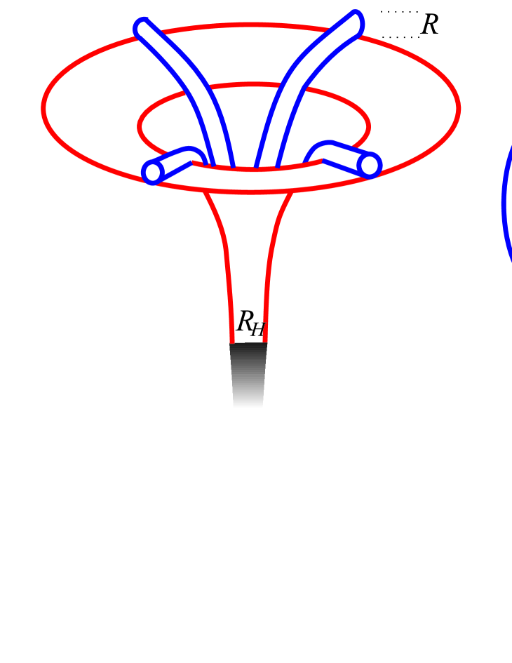
Figure 3: Sketch of the black hole topology in a space time with compactified extra dimensions. The left picture shows the astrophysical black hole with $R_{H}\gg R$, the right picture shows the collider produced black hole with $R_{H}\ll R$.

The higher dimensional Schwarzschild-metric has been derived in [21] and takes the form

$${\rm d}s^{2}=-\gamma(r){\mathrm{d}}t^{2}+\gamma^{-1}(r){\mathrm{d}}r^{2}+r^{2}{\mathrm{d}}\Omega^{2}_{(d+3)}\quad,$$ (34)

where ${\rm d}\Omega_{(d+3)}$ now is the surface element of the $3+d$ - dimensional unit sphere and

$$\gamma(r)=1-\left(\frac{R_{H}}{r}\right)^{d+1}\quad.$$ (35)

The constant $R_{H}$ again can be found by requiring that we reproduce the Newtonian limit for $r\gg R$, that is $1/2\partial_{r}\gamma$ has to yield the Newtonian potential:

$$\frac{d+1}{2}\left(\frac{R_{H}}{r}\right)^{1+d}\frac{1}{r}=\frac{1}{M_{\rm f}^{d+2}}\frac{M}{r^{d+2}}\quad.$$ (36)

So we have

$$\gamma(r)=1-\frac{2}{d+1}\frac{1}{M_{\rm f}^{d+2}}\frac{M}{r^{d+1}}\quad,$$ (37)

and $R_{H}$ is

$$R_{H}^{d+1}=\frac{2}{d+1}\left(\frac{1}{M_{\rm f}}\right)^{d+1}\;\frac{M}{M_{\rm f}}\;\;.$$ (38)

It is not surprising to see that a black hole with a mass about the new fundamental mass $M\sim M_{\rm f}$, has a radius of about the new fundamental length scale $L_{\rm f}=1/M_{\rm f}$ (which justifies the use of the limit $R_{H}\ll R$). For $M_{\rm f}\sim$ 1TeV this radius is $\sim 10^{-4}$ fm. Thus, at the LHC it would be possible to bring particles closer together than their horizon. A black hole could be created.

The surface gravity can be computed using Eq.(12)

$$\kappa=\frac{1+d}{2}\frac{1}{R_{H}}\quad,$$ (39)

and the surface of the horizon is now given by

$${\cal{A}} = \Omega_{(d+3)}R_{H}^{d+2}$$ (40)

$$= \Omega_{(d+3)}\frac{M}{\kappa}\left(\frac{1}{M_{\rm f}}\right)^{d+2}\quad,$$ (41)

where $\Omega_{(d+3)}$ is the surface of the $d+3$-dimensional unit sphere.

$$\Omega_{(d+3)}=\frac{2\pi^{\frac{d+3}{2}}}{\Gamma({\frac{d+3}{2}})}\;\;.$$ (42)

figure

Schematic figure for a particle collision. At very high energies, the particles, $p$, can come closer than the Schwarzschild radius, $R_{H}$, associated with their energy. If the impact parameter, $b$, is sufficiently small, such a collision will inevitably generate a trapped surface. A black hole has been created.

5.1 Production of Black Holes

Let us consider two elementary particles, approaching each other with a very high kinetic energy in the c.o.m. system close to the new fundamental scale $M_{\rm f}\sim 1$ TeV, as depicted in Figure 5. At those high energies, the particles can come very close to each other since their high energy allows a tightly packed wave package despite the uncertainty relation. If the impact parameter is small enough, which will happen to a certain fraction of the particles, we have the two particles plus their large kinetic energy in a very small region of space time. If the region is smaller than the Schwarzschild radius connected with the energy of the partons, the system will collapse and form a black hole.

The production of a black hole in a high energy collision is probably the most inelastic process one might think of. Since the black hole is not an ordinary particle of the Standard Model and its correct quantum theoretical treatment is unknown, it is treated as a metastable state, which is produced and decays according to the semi classical formalism of black hole physics.

To compute the production details, the cross-section of the black holes can be approximated by the classical geometric cross-section

$$\sigma(M)\approx\pi R_{H}^{2}\quad,$$ (43)

an expression which does only contain the fundamental Planck scale as coupling constant. This cross section has been under debate [22], but further investigations justify the use of the classical limit at least up to energies of $\approx 10M_{\rm f}$ [23]. However, the topic is still under discussion, see also the very recent contributions [24].

A common approach to improve the naive picture of colliding point particles, is to treat the creation of the horizon as a collision of two shock fronts in an Aichelburg-Sexl geometry describing the fast moving particles [25]. Due to the high velocity of the moving particles, space time before and after the shocks is almost flat and the geometry can be examined for the occurrence of trapped surfaces.

These semi classical considerations do also give rise to form factors which take into account that not the whole initial energy is captured behind the horizon. These factors have been calculated in [26], depend on the number of extra dimensions, and are of order one. For our further qualitative discussion we will neglect them. A time evolution of the system forming the black hole is not provided is this treatment but it has been shown that the naively expected classical result remains valid also in String Theory [27].

Looking at Figure 5, we also see that, due to conservation laws, the angular momentum $J$ of the formed object only vanishes in completely central collisions with zero impact parameter, $b=0$. In the general case, we will have an angular momentum $J\approx 1/2Mb$. However, this modification turns out to be only about a factor $2$ [28]. In general, the black hole will also carry a charge which gives rise to the exciting possibility of naked singularities. We will not further consider this case here, the interested reader is referred to [29].

Another assumption which goes into the production details is the existence of a threshold for the black hole formation. From General Relativistic arguments, two point like particles in a head on collision with zero impact parameter will always form a black hole, no matter how large or small their energy. At small energies, however, we expect this to be impossible due to the smearing of the wave functions by the uncertainty relation. This then results in a necessary minimal energy to allow for the required close approach. This threshold is of order $M_{\rm f}$, though the exact value is unknown since quantum gravity effects should play an important role for the wave functions of the colliding particles. For simplicity, we will in the following set this threshold equal to $M_{\rm f}$ but we want to point out that most of the analysis in the literature assumes a parameter of order one.

This threshold is also important as it defines the window in which other effects of the LXD scenario can be observed. Besides the graviton production and the excitation of KK-modes, also string excitations [30] have been examined. At even higher energies, highly exited long strings, the stringballs [31], are expected to dominate the scattering process. At the threshold energy, the so called correspondence point, the excited states can be seen either as strings or as black holes [32]. The smooth transition from strings to black holes has recently been investigated in Ref. [33]. The occurrence of these string excitations can increase the transverse size of the colliding objects and thus, make black hole production more difficult. This important point will be further discussed in Section 7.

Setting $M_{\rm f}\sim 1$TeV and $d=2$ one finds $\sigma\sim 400$ pb. Using the geometrical cross section formula, it is now possible to compute the differential cross section ${\mathrm{d}}\sigma/{\mathrm{d}}M$ which will tell us how many black holes will be formed with a certain mass $M$ at a c.o.m. energy $\sqrt{s}$. The probability that two colliding particles will form a black hole of mass $M$ in a proton-proton collision at the LHC involves the parton distribution functions. These functions, $f_{A}(x,\hat{s})$, parametrize the probability of finding a constituent $A$ of the proton (quark or gluon) with a momentum fraction $x$ of the total energy of the proton. These constituents are also called partons. Here, $\sqrt{\hat{s}}$ is the c.o.m. energy of the parton-parton collision.

The differential cross section is then given by summation over all possible parton interactions and integration over the momentum fractions, where the kinematic relation $x_{1}x_{2}s=\hat{s}=M^{2}$ has to be fulfilled. This yields

$$\frac{{\rm d}\sigma}{{\rm d}M} = \sum_{A_{1},B_{2}}\int_{0}^{1}{\rm d}x_{1}\frac{2\sqrt{\hat{s}}}{x_{1}s}f_{A}(x_{1},\hat{s})f_{B}(x_{2},\hat{s})\sigma(M,d)\quad.$$ (44)

The particle distribution functions for $f_{A}$ and $f_{B}$ are tabulated e.g. in the CTEQ - tables. A numerical evaluation of this expression results in the differential cross section displayed in Figure 4, left. Most of the black holes have masses close to the production threshold. This is due to the fact that at high collision energies, or small distances respectively, the proton contents a high number of gluons which dominate the scattering process and distribute the total energy among themselves.

Figure 4: The left plot shows the differential cross section for black hole production in proton-proton-collisions at the LHC for $M_{\rm f}=1$ TeV. The right plot shows the integrated total cross section as a function of the collision energy $\sqrt{s}$. In both cases, the curves for various $d$ differ from the above depicted ones by less than a factor 10.

It is now straightforward to compute the total cross section by integration over Eq. (44), see Figure 4, right. This also allows us to estimate the total number of black holes, $N_{\rm BH}$, that would be created at the LHC per year. It is $N_{\rm BH}/{\rm year}=\sigma(pp\to{\rm BH})L$ where we insert the estimated luminosity for the LHC, $L=10^{33}{\rm cm}^{-2}{\rm s}^{-1}$. This yields at a c.o.m. of $\sqrt{s}=14$ TeV a number of $N_{\rm BH}\approx 10^{9}$ per year! This means, about one black hole per second would be created. This result does also agree with the values found in [34]. The importance of this process led to a high number of publications on the topic of TeV-mass black holes at colliders [34, 35, 36, 37, 38, 39, 40, 41, 42].

The here presented calculation applies for the Large Hadron Collider and uses the parton distribution functions. At such high energies, these functions are extrapolations from low energy measurements and one might question whether the extrapolation can be applied into the regime of quantum gravity, or whether additional effects might modify them. Modifications might e.g. arise through the occurrence of a minimal length scale [43] or the presence of virtual graviton or KK-excitations. One should also keep in mind that the used extrapolations, the DGLAP equations [44], rely on sliding scale arguments similar to the running of the coupling constants which is known to be modified in the presence of extra dimensions [45].

In this context it is therefore useful to examine black hole production at lepton colliders, which excludes the parton distribution functions as a source of uncertainty. A recent analysis has been given by in [42] for a muon collider. In general, the number for the expected black hole production at lepton colliders will be higher than for hadron colliders at equal energies, which is due to the collision energy not being distributed among the hadron constituents.

High energetic collision with energies close by or even above the new fundamental scale could also be reached in cosmic ray events [19]. Horizontally infalling neutrinos, which are scattered at nuclei in the atmosphere are expected to give the most important and clearest signature.

5.2 Evaporation of Black Holes

One of the primary observables in high energetic particle collisions is the transverse momentum of the outgoing particles, $p_{T}$, the component of the momentum transverse to the direction of the beam. Two colliding partons with high energy can produce a pair of outgoing particles, moving in opposite directions with high $p_{T}$ but carrying a color charge, as depicted in Figure 5.2, top. Due to the quark confinement, the color has to be neutralized. This results in a shower of several bound states, the hadrons, which includes mesons (consisting of a quark and an antiquark, like the $\pi$’s) as well as baryons (consisting of three quarks, like the neutron or the proton). The number of these produced hadrons and their energy depends on the energy of the initial partons. This process will cause a detector signal with a large number of hadrons inside a small opening angle. Such an event is called a ’jet’.

Typically these jets come in pairs of opposite direction. A smaller number of them can also be observed with three or more outgoing showers. This observable will be strongly influenced by the production of black holes.

To understand the signatures that are caused by the black holes we have to examine their evaporation properties. As we have seen before, the smaller the black hole, the larger is its temperature and so, the radiation of the discussed tiny black holes is the dominant signature caused by their presence. As we see from Eq. (39) and Eq. (13) the typical temperature lies in the range of several $100$ GeV. Since most of the particles in the black body radiation are emitted with this average energy, we can estimate the total number of emitted particles to be of order $10$-$100$. As we will see, this high temperature results in a very short lifetime such that the black hole will decay close by the collision region and can be interpreted as a metastable intermediate state.

figure

Phases of black hole evaporation.

Once produced, the black holes will undergo an evaporation process whose thermal properties carry information about the parameters $M_{\rm f}$ and $d$. An analysis of the evaporation will therefore offer the possibility to extract knowledge about the topology of our space time and the underlying theory.

The evaporation process can be categorized in three characteristic stages [36], see also the illustration in Figure 5.2:

1. Balding phase: In this phase the black hole radiates away the multipole moments it has inherited from the initial configuration, and settles down in a hairless state. During this stage, a certain fraction of the initial mass will be lost in gravitational radiation.

2. Evaporation phase: The evaporation phase starts with a spin down phase in which the Hawking radiation carries away the angular momentum, after which it proceeds with emission of thermally distributed quanta until the black hole reaches Planck mass. The radiation spectrum contains all Standard Model particles, which are emitted on our brane, as well as gravitons, which are also emitted into the extra dimensions. It is expected that most of the initial energy is emitted in during this phase in Standard Model particles.

3. Planck phase: Once the black hole has reached a mass close to the Planck mass, it falls into the regime of quantum gravity and predictions become increasingly difficult. It is generally assumed that the black hole will either completely decay in some last few Standard Model particles or a stable remnant will be left, which carries away the remaining energy.

The evaporation rate ${\rm d}M/{\rm d}t$ of the higher dimensional black hole can be computed using the thermodynamics of black holes. With Eq. (39), (41) and (12) we find for the temperature of the black hole

$$T=\frac{1+d}{4\pi}\frac{1}{R_{H}}\quad,$$ (45)

where $R_{H}$ is a function of $M$ by Eq. (38). Integration of the inverse temperature over $M$ then yields (compare to Eq.(16))

$$S(M) = 2\pi\frac{d+1}{d+2}\left(M_{\rm f}R_{H}\right)^{d+2}\quad.$$ (46)

For the spectral energy density we use the micro canonical particle spectra Eq. (22) and (23) but we now have to integrate over the higher dimensional momentum space

$$\varepsilon=\frac{\Omega_{(d+3)}}{(2\pi)^{3+d}}{\mathrm{e}}^{-S(M)}\sum_{j=1}^{\infty}\frac{1}{j^{d+4}}\int_{0}^{M}{\mathrm{e}}^{S(x)}(M-x)^{3+d}{\mathrm{d}}x\quad,$$ (47)

where the value of the sum is given by a $\zeta$-function. From this we obtain the evaporation rate

$$\frac{{\mathrm{d}}M}{{\mathrm{d}}t}=\frac{\Omega_{(d+3)}^{2}}{(2\pi)^{d+3}}R_{H}^{2+d}\zeta(4+d)\;{\rm e}^{-S(M)}\int_{0}^{M}(M-x)^{(3+d)}{\rm e}^{S(x)}{\mathrm{d}}x\quad.$$ (48)

A plot of this quantity for various $d$ is shown in Figure 5, left. The mass dependence resulting from it is shown in Figure 5, right. We see that the evaporation process slows down in the late stages and enhances the life time of the black hole.

Figure 5: The left plot shows the evaporation rate in as a function of the initial mass for various $d$. The right plot shows the time evolution of a black hole with an initial mass of 10 TeV.

To perform a realistic simulation of the evaporation process, one has to take into account the various particles of the Standard Model with the corresponding degrees of freedom and spin statistics. In the extra dimensional scenario, Standard Model particles are bound to our submanifold whereas the gravitons are allowed to enter all dimensions. It has been argued that black holes emit mainly on the brane [35]. The ratio between the evaporation in the bulk and in the brane can be estimated by applying Eq. (48) to $3$ or $3+d$ dimensions, respectively. For simplicity we will assume that the mass is high enough such that the result approximately agrees with the higher dimensional Stefan-Bolzmann law. Then it is

$$\frac{{\mathrm{d}}M}{{\mathrm{d}}t} = \frac{\Omega_{(3)}^{2}}{(2\pi)^{3}}R_{H}^{2}\zeta(4)\Gamma(4)\;T^{4}\quad{\mbox{on the brane, and}}$$ (49)

$$\frac{{\mathrm{d}}M}{{\mathrm{d}}t} = \frac{\Omega_{(3+d)}^{2}}{(2\pi)^{3+d}}R_{H}^{2+d}\zeta(4+d)\Gamma(4+d)\;T^{4+d}\quad{\mbox{in the bulk,}}$$ (50)

which yields a ratio brane/bulk of

$$\frac{\Omega_{(3)}^{2}}{\Omega_{(3+d)}^{2}}\frac{\zeta(4)}{\zeta(4+d)}\frac{\Gamma(4)}{\Gamma(4+d)}\left(\frac{2\pi}{TR_{H}}\right)^{d}\quad.$$ (51)

Inserting Eq. (45) results in a ratio, dependent on $d$, which is of order $4-12$, for $d\leq 7$ with a maximum for $d=4$. In addition one has to take into account that there exists a much larger number of particles in the Standard Model than those which are allowed in the bulk. Counting up all leptons, quarks, gauge bosons, their anti particles and summing over various quantum numbers yields more than $60$. This has to be contrasted with only one graviton in the bulk which strongly indicates that most of the radiation goes into the brane.

However, the exact value will depend on the correct spin statistics and in general, the ratio also depends on the temperature of the black hole as can e.g. be seen in Figure 5, left. We also see that for masses close to the new fundamental scale the evaporation rate is higher for a smaller number of extra dimensions. This is due to the fact that in this region the evaporation rate is better approximated by a higher dimensional version of Wien’s law. For a precise calculation one also has to take into account that the presence of the gravitational field will modify the radiation properties for higher angular momenta through backscattering at the potential well. These energy dependent greybody factors can be calculated by analyzing the wave equation in the higher dimensional spacetime and the arising absorption coefficients. A very thorough description of these evaporation characteristics has been given in [10] which confirms the expectation that the bulk/brane evaporation rate is of comparable magnitude but the brane modes dominate.

For recent reviews on TeV-scale black holes see also [46] and references therein.

5.3 Observables of Black Holes

Due to the high energy captured in the black hole, the decay of such an object is a very spectacular event with a distinct signature. The number of decay products, the multiplicity, is high compared to Standard Model processes and the thermal properties of the black hole will yield a high sphericity of the event. Furthermore, crossing the threshold for black hole production causes a sharp cut-off for high energetic jets as those jets now end up as black holes instead, and are re-distributed into thermal particles of lower energies. Thus, black holes will give a clear signal.

It is apparent that the consequences of black hole production are quite disastrous for the future of collider physics. Once the collision energy crosses the threshold for black hole production, no further information about the structure of matter at small scales can be extracted. As it was put by Giddings and Thomas [36], this would be ”the end of short distance physics”.

Figure 6: Left: The onset of black hole production in high energy collisions results in a cut off for high $p_{T}$-jets. Here, it is $\sqrt{s}=14$ TeV and $M_{\rm f}=1$ TeV. The average over the rapidity region $|y|\leq 1$ is taken. Right: This plot from [41] shows the multiplicity of black hole events for various numbers of extra dimensions $d=$ 2 (black), 3 (green), 4 (red), 5 (cyan) and 6 (blue).

Figure 6, left shows the expected cross section for jets at high transverse momentum with an onset of black hole production in comparison to the perturbative QCD prediction. The cutoff is close by the new fundamental scale but is hardly sensitive to the number of extra dimensions.

By now, several experimental groups include black holes into their search for physics beyond the Standard Model. PYTHIA 6.2 [47] and the CHARYBDIS [48] event generator allow for a simulation of black hole events and data reconstruction from the decay products. Such analysis has been summarized in Ref. [40] and Ref. [41], respectively. Ideally, the energy distribution of the decay products allows a determination of the temperature (by fitting the energy spectrum to the predicted shape) as well as of the total mass of the object (by summing up all energies). This then allows to reconstruct the scale $M_{\rm f}$ and the number of extra dimensions. An example for this is shown in Figure 5.3, from [34].

The quality of the determination, however, depends on the uncertainties in the theoretical prediction as well as on the experimental limits e.g. background from Standard Model processes. Besides the formfactors of black hole production and the greybody factors of the evaporation, the largest theoretical uncertainties turn out to be the final decay and the time variation of the temperature. In case the black hole decays very fast, it can be questioned [34] whether it has time to readjust its temperature at all or whether it essentially decays completely with its initial temperature.

Also, the determination of the properties depends on the number of emitted particles. The less particles, the more difficult the analysis.

Figure 6 right, from [41], shows the number of expected decay products of a black hole event. For larger $d$ with a fixed mass, the temperature increases which leads to less higher energetic particles. In Ref. [41] it was also pointed out that the high sphericity even at low multiplicity allows clear distinction from Standard Model and/or SUSY events. In a simulated test case, it was found that the fundamental scale can be determined up to 15% and the number of extra dimensions up to $\pm$0.75.

figure

[h]

This plot from [34] shows an example for a reconstruction of the parameters from simulated black hole events. Here, it was assumed that the black hole decays so fast that the temperature can not be readjusted and is therefore time independent.

6 Black Hole Relics

The final fate of these small black holes is difficult to estimate. The last stages of the evaporation are closely connected to the information loss puzzle. The black hole emits thermal radiation, whose sole property is the temperature, regardless of the initial state of the collapsing matter. So, if the black hole completely decays into statistically distributed particles, unitarity can be violated. This happens when the initial state is a pure quantum state and then evolves into a mixed state [5, 49, 51].

When one tries to avoid the information loss problem two possibilities are left. The information is regained by some unknown mechanism or a stable black hole remnant is formed which keeps the information. Besides the fact that it is unclear in which way the information should escape the horizon [52] there are several other arguments for black hole relics [53]:

• The uncertainty relation: The Schwarzschild radius of a black hole with Planck mass is of the order of the Planck length. Since the Planck length is the wavelength corresponding to a particle of Planck mass, a problem arises when the mass of the black hole drops below Planck mass. Then one has trapped a higher mass, $M\geq M_{\rm f}$, inside a volume which is smaller than allowed by the uncertainty principle [54]. To avoid this problem, Zel’dovich has proposed that black holes with masses below Planck mass should be associated with stable elementary particles [55].

• Corrections to the Lagrangian: The introduction of additional terms, which are quadratic in the curvature, yields a dropping of the evaporation temperature towards zero [56, 57]. This holds also for extra dimensional scenarios [58] and is supported by calculations in the low energy limit of string theory [59, 60].

• Further reasons for the existence of relics have been suggested to be black holes with axionic charge [61], the modification of the Hawking temperature due to quantum hair [62] or magnetic monopoles [63]. Coupling of a dilaton field to gravity also yields relics, with detailed features depending on the dimension of space-time [64, 65].

Of course these relics, which have also been termed Maximons, Friedmons, Cornucopions, Planckons or Informons, are not a miraculous remedy but bring some problems on their own. Such is e.g. the necessity for an infinite number of states which allows the unbounded information content inherited from the initial state.

However, let us consider a very simple model which will help us to understand the features which lead to the formation of a stable black hole remnant. We will suppose that the spectrum of the radiation emitted by the black hole is discretized by geometrical means. The smaller the black hole is, the smaller is the region of space time out of which the radiation emerges and we expect the finite size of the black hole to reflect in the features of the radiation. The details of this ansatz have been worked out in [66].

In particular, for the derivation of the black hole’s Hawking radiation, it turns out that the black hole acts like a black body. These analogy to geometrical optics can be put even further, see e.g. [50].

We split the solution for the $d+3$ dimensional wave equation of the black hole modes into an amplitude proportional to $\propto 1/r^{d+1}$, an angular dependence and a radial part. We then assume that the spectrum of the modes can only have discrete values due to the geometric boundary conditions $k_{l}=\pi l/R_{H}$, as depicted in Figure 6.

figure

[h]

The black hole can not emit wave length that do not fit to the horizon size. The spectrum of the radiation is geometrically quantized in discrete steps. If the black hole shrinks, the lowest energetic mode can already exceed the total energy and thus, can not be emitted.

The particle spectrum Eq. (23) is then replaced by a spectrum for the discrete energy values $\omega_{l}=l\Delta\omega$ with step size $\Delta\omega=\pi/R_{H}$

$$n(l)=\sum_{j=1}^{\lfloor\frac{M}{l\Delta\omega}\rfloor}\frac{{\rm exp}[S(M-jl\Delta\omega)]}{{\rm exp}[S(M)]}\Theta\left(M-l\Delta\omega\right)\quad.$$ (52)

Here, the Heaviside-function $\Theta$ cuts off the sum when the energy of one particle ($j=1$) exceeds the whole mass of the black hole. The energy density is then given by a summation instead of an integration

$$\varepsilon = \frac{\Omega_{(d+3)}}{(2\pi)^{3+d}}\Delta\omega\sum_{l=1}^{\lfloor\frac{M}{\Delta\omega}\rfloor}n(l)\left(l\Delta\omega\right)^{d+3}\;\;,$$ (53)

which does as before result in an expression for the evaporation rate. For large masses, $M\gg M_{\rm f}$, the sum becomes an integral and Eq.(53) reduces to the continuous case. Figure 7, left, shows the evaporation rate with geometrical quantization in contrast to the continuous result (compare to Figure 5).

Figure 7: The left plot[66] shows the evaporation rate with discrete energy spectrum in comparison to the continuous case (dotted) for various $d$. The right plot, from [43], shows the total cross section for black hole production as a function of the center of mass energy $\sqrt{s}$ with and without the generalized uncertainty principle (GUP). For the expected LHC-energies the cross sections is lowered by about a factor 5. This result does barely depend on the number of extra dimensions.

With increasing $M$, the steps between the energy levels become smaller. If it is possible to occupy an additional level, the evaporation rate has a step. In the mass region of interest for us, it is $R_{H}\approx 1/M_{\rm f}$ and thus the steps are $\approx\pi$TeV.

The lowest energetic mode possible corresponds to the largest wavelength which fits into the black holes horizon. The smaller the black hole is, the smaller this wavelength has to be and thus, the energy of the lowest level increases. At black hole masses close to the Planck mass, it happens that even the energy of the lowest level would exceed the total energy of the black hole and can not be emitted.

The evaporation therefore will proceed in quantized steps and stops at a finite mass value. A relic is left.

The production of a relic instead of a final decay of the black hole would increase the missing $p_{T}$ in the particle collision. Also, a certain fraction of these objects will be charged which allows for a direct detection.

7 The Minimal Length

Gravity itself is inconsistent with physics at very short scales. The introduction of gravity into into quantum field theory appears to spoil their renormalizability and leads to incurable divergences. It has therefore been suggested that gravity should lead to an effective cutoff in the ultraviolet, i.e. to a minimal observable length. It is amazing enough that all attempts towards a fundamental theory of everything necessarily seem to imply the existence of such a minimal length scale.

The occurrence of the minimal length scale has to be expected from very general reasons in all theories at high energies which attempt to include effects of quantum gravity. This can be understood by a phenomenological argument which has been examined in various ways. Test particles of a sufficiently high energy to resolve a distance as small as the Planck length, $l_{\rm p}=1/m_{\rm p}$, are predicted to gravitationally curve and thereby to significantly disturb the very spacetime structure which they are meant to probe. Thus, in addition to the expected quantum uncertainty, there is another uncertainty caused which arises from spacetime fluctuations at the Planck scale.

Consider a test particle, described by a wave packet with a mean Compton-wavelength $\lambda$. Even in standard quantum mechanics, the particle suffers from an uncertainty in position $\Delta x$ and momentum $\Delta p$, given by the standard Heisenberg-uncertainty relation $\Delta x\Delta p\geq 1/2$. Usually, every sample under investigation can be resolved by using beams of high enough momentum to focus the wave packet to a width below the size of the probe, $\Delta x$, which we wish to resolve. The smaller the sample, the higher the energy must become and thus, the bigger the collider.

General Relativity tells us that a particle with an energy-momentum $p\sim 1/\lambda$ in a volume of spacetime $\Delta x^{3}$ causes a fluctuation of the metric $g$. Einstein’s Field Equations (1) allow us to relate the second derivative of the metric to the energy density and so we can estimate the perturbation with

$$\frac{\delta g}{\Delta x^{2}}\sim l_{\rm p}^{2}\frac{p}{\Delta x^{3}}\quad.$$ (54)

This leads to an additional fluctuation, $\Delta x^{\prime}$, of the spacetime coordinate frame of order $\Delta x^{\prime}=\delta g\Delta x\approx l_{\rm p}^{2}p$, which increases with momentum and becomes non-negligible at Planckian energies.

But from this expression we see not only that the fluctuations can no longer be neglected at Planckian energies and the uncertainty of the measurement is amplified. In addition, we see that a focussation of energy of the amount necessary to resolve the Planck scale leads to the formation of a black hole whose horizon is located at $\delta g\approx 1$, should the matter be located inside. Since the black hole radius has the property to expand linearly with the energy inside the horizon, both arguments lead to the same conclusion: a minimal uncertainty in measurement can not be erased by using test particles of higher energies. It is always $\Delta x>l_{\rm p}$: at low energies because the Compton-wavelengths are too big for a high resolution, at high energies because of strong curvature effects.

Thus, to first order the uncertainty principle is generalized to

$$\Delta x\gtrsim\frac{1}{\Delta p}+\mbox{const.}~{}~{}l_{\rm p}^{2}{p}\quad.$$ (55)

Without doubt, the Planck scales marks a thresholds beyond which the old description of space-time breaks down and new phenomena have to appear.

More stringent motivations for the occurrence of a minimal length are manifold. A minimal length can be found in String Theory, Loop Quantum Gravity and Non-Commutative Geometries. It can be derived from various studies of thought-experiments, from black hole physics, the holographic principle and further more. Perhaps the most convincing argument, however, is that there seems to be no self-consistent way to avoid the occurrence of a minimal length scale. For reviews see e.g. [67].

Instead of finding evidence for the minimal scale as has been done in numerous studies, on can use its existence as a postulate and derive extensions to quantum theories with the purpose to examine the arising properties in an effective model.

Such approaches have been undergone and the analytical properties of the resulting theories have been investigated closely [68]. In the scenario without extra dimensions, the derived modifications are important mainly for structure formation and the early universe [69].

The importance to deal with a finite resolution of spacetime, however, is sensibly enhanced if we consider a spacetime with large extra dimensions. In this case, the new fundamental mass scale is lowered and thus, the minimal length is raised. The effects of a finite resolution of spacetime should thus become important in the same energy range in which the first effects of gravity are expected. Some consequences of the inclusion of the minimal length into the model of extra dimensions have been worked out in [70].

figure

[h]

A generalized uncertainty principle, as follows from the existence of a minimal length scale, makes it increasingly difficult to focus the wave functions of the colliding particles. This is sketched in Figure 7. It requires higher energies to achieve an energy density inside the Schwarzschild radius which is sufficient for a collapse and the creation of a black hole.

The consequences of the generalized uncertainty for the total black hole cross section and the number of produced black holes have been derived in [43] and are depicted in Figure 7, right. As we expect, the cross section is lowered. For the estimated LHC-energies this results in a suppression of the black hole production by a factor $\approx 5$.

Schematic figure for parton scattering with and without generalized uncertainty .

The arising modifications at high energies do also influence the production of black holes. Using the generalized uncertainty principle, the properties [39] of the evaporation process are modified when the black hole radius approaches the minimal length which decreases the number of decay particles and leads to the formation of a stable remnant.

8 Are Those Black Holes dangerous?

”Big Bang Machine: Will it destroy Earth?, Creation of a black hole on Long Island?

The committee will also consider […] that the colliding particles could achieve such a high density that they would form a mini black hole. In space, black holes are believed to generate intense gravitational fields that suck in all surrounding matter. The creation of one on Earth could be disastrous. […]”

The London Times, July 18th, 1999

Considered the fact that black holes are known to swallow whole galaxy centers, the question might be raised whether the tiny black holes, produced in the laboratory, would also accrete mass, swallow it and grow until everything in reach would be vanished beyond the event horizon.

Fortunately, this question can without doubt be answered with ’No’. These earth produced black holes still have a very small gravitational attraction. An energy of some TeV might be huge for collider physics but for gravitational purposes it is tiny. The strength of the gravitational force, acting on electrons orbiting around a nucleus, is even in the presence of extra dimensions still by a factor $\approx 10^{20}$ weaker than the electromagnetic force.

We can estimate the possibility of black holes gaining mass based on our earlier given results. Looking at Figure 5, we see that the mass loss ratio, ${\rm d}M_{-}/{\rm d}t$ of the black hole is at least $\approx 1$ TeV $c$/fm, for a large number of extra dimensions it would be even larger. As previously stated, the gravitational attraction of the black hole is negligible. Nevertheless, is the black hole placed in a medium which is considered to be extremely dense and hot in earthly terms, it will gain mass by particles crossing the horizon simply through thermal motion. This mass gain ratio can be estimated to be

$$\frac{dM_{+}}{dt}\sim\pi R_{H}^{2}T_{\rm m}^{4}\quad,$$ (56)

where $T_{\rm m}$ is the temperature of the medium and the fore-factor is the surface of the black hole as seen on our submanifold. Inserting $\rho=T_{\rm m}^{4}$ to be the most dense medium produced on earth, e.g. a Quark Gluon Plasma, we have typically $\rho\sim 100$ MeV/fm³. Using as a characteristic value $R_{H}=1/M_{\rm f}\sim 1/$TeV, we find that

$$\frac{{\rm d}M_{+}}{{\rm d}t}\sim 10^{-9}\frac{{\rm GeV}c}{\rm fm}\ll\frac{{\rm d}M_{-}}{{\rm d}t}\quad,$$ (57)

and so the black hole will loose mass much faster than it can gain mass.

Let us consider a further extreme case: a black hole, created by an ultra high high energetic cosmic ray, which traverses a neutron star. Cosmic ray events can occur at energies as high as $10^{8}$ TeV and thus, can yield black holes with an ultra high $\gamma$-factor, $\gamma\sim E/M\sim 10^{7}$. This means, the black hole has an ultra high speed and due to the effects of Lorentz-contraction, it will see the medium of the neutron star in an even higher density. Or, to put it different, in the reference frame of the neutron star the black hole travels fast, undergoes the relativistic time dilation and evaporates slower.

In the reference frame of the black hole, the mass loss is still given by the above estimation but it now sees a medium with density $\gamma^{2}\rho$. The mass gain during passage of the neutron star is then increased by a factor $\gamma^{2}\sim 10^{14}$. By multiplying Eq. (57) with this factor we see that in this case, the mass gain become comparable to the mass loss! The black hole thus has a chance to eat up a significant part of the neutron star. This process has been investigated in [71]. However, the estimation we have given here does only apply immediately after the creation of the black hole. Once it starts growing, it will become more massive and slow down. This in turn will decrease its $\gamma$-factor, the mass loss again becomes dominant and the black hole decays. A continuing growth is possible only in a very constrained parameter range which is already excluded [71].

Prejudices against Black Holes
Black holes are mathematical trash: Wrong! The existence of an event horizon is a perfectly well defined space time property. Moreover, their formation follows from such general assumptions that to present knowledge there is no way to avoid them. General Relativity requires black holes. Since the horizon radius is proportional to the mass $M$, it follows that the density needed for the horizon formation is proportional to $M/M^{3}$. This means, for large masses, the density can be arbitrarily small.
Black holes are speculative: Wrong! The evidence for a black hole in the center of our galaxy (Sag. A^∗) is overwhelming [72]. More than 20 other candidates in our galaxy [73] and 10 further super massive black holes [74] have been established so far. The analysis of the motion of the surrounding objects is used to determine the amount mass concentrated in their vicinity. The mass inside the region is so high that the only plausible explanation is a black hole and everything else is highly speculative [75].
Black holes are black: Wrong! The strong curvature effects in the vicinity of a black hole can rip apart virtual particle pairs and result in particle emission in the Hawking-radiation process. For objects of astrophysical sizes, this temperature is too low to be observable. These large black holes in general have rotating accretion disks surrounding them, in which the fast moving matter gets extremely hot and emits radiation.
Black holes on earth are dangerous: Wrong! The black holes which could possibly be created on earth would still have a very small mass and, connected with it, a very small gravitational attraction. Their interaction with other particles is so weak that they can not grow, even under extreme conditions, like inside a quark gluon plasma. In all cases, the evaporation processes will dominate, causing the black hole to decay instead to grow.

9 Summary: What Black Holes Can Teach Us

Black holes are a topic as fascinating as challenging. The investigations during the last century have led to important insights. Thermodynamics of black holes taught us of a deep connection between quantum theory, General Relativity and thermodynamics which has recently been studied further in the string/black hole correspondence and is a matter of ongoing research. Black holes and the puzzle of information loss have tought us about the possibility of stable black hole relics and the natural inclusion of a minimal length scale.

The presence of additional compactified dimensions would allow the production of tiny black holes in particle collisions. Their investigation in experiments on earth would provide a direct possibility to address the question of extra dimensions and the new fundamental scale. But moreover, it would allow us to probe the phenomenology of physics at the Planck scale and increase our knowledge about the underlying, yet to be found theory. Black holes can teach us to find the missing link between general relativity and quantum theory.

Acknowledgments

I want to thank Marcus Bleicher, Stefan Hofmann and Horst Stöcker for the inspiring discussions at Frankfurt University. I also thank Claudia Schumacher for critical remarks. I apologize for every missing citation on the topic. This work was supported by the German Academic Exchange Service (DAAD), NSF PHY/0301998 and the DFG.

Appendix A Useful Fomulae

$$\Gamma^{\alpha}_{\;\;\;\mu\nu} = \frac{1}{2}g^{\alpha\beta}(\partial_{\mu}g_{\beta\nu}+\partial_{\nu}g_{\beta\mu}-\partial_{\nu}g_{\mu\nu})$$ (58)

$$R^{\mu}_{\;\;\;\nu\alpha\beta} = \partial_{\alpha}\Gamma^{\mu}_{\;\;\;\nu\beta}-\partial_{\alpha}\Gamma^{\mu}_{\;\;\;\nu\alpha}+\Gamma^{\mu}_{\;\;\;\rho\alpha}\Gamma^{\rho}_{\;\;\;\nu\beta}-\Gamma^{\mu}_{\;\;\;\rho\beta}\Gamma^{\rho}_{\;\;\;\nu\alpha}$$ (59)

$$R^{\mu}_{\;\;\;\nu} = R^{\alpha}_{\;\;\;\mu\alpha\nu}$$ (60)

$$R = g^{\mu\nu}R_{\mu\nu}$$ (61)

Appendix B Useful Constants

Planck length	$l_{\rm p}$	$\approx$	$10^{-35}$ m	$\approx$	$10^{-20}$ fm
Planck mass	$m_{\rm p}$	$\approx$	$10^{-5}$ g	$\approx$	$1.2\times 10^{16}$ TeV
Planck time	$t_{\rm p}$	$\approx$	$10^{-43}$ s	$\approx$	$10^{-20}$ fm/$c$
Mass of the sun	$M_{\odot}$	$\approx$	$2\times 10^{33}$ g	$\approx$	$2.4\times 10^{54}$ TeV
Radius of the sun	$R_{\odot}$	$\approx$	$7\times 10^{8}$ m
Schwarzschild
radius of the Sun	$R_{H}$	$\approx$	$3\times 10^{3}$ m
c.o.m. energy
at the LHC	$\sqrt{s}$			$\approx$	14 TeV

References

- [1] K. Schwarzschild, ”Über das Gravitationsfeld eines Massenpunktes nach der Einsteinschen Theorie” in ”Sitzungsberichte der Königlich Preussischen Akademie der Wissenschaften zu Berlin”, 189-196 (1916).
- [2] C. W. Misner, K. S. Thorne and J. A. Wheeler, ”Gravitation”, W. H. Freeman and Company (New York, 1973); R. U. Sexl and H. K. Urbantke, ”Gravitation Und Kosmologie””, Spektrum Akademischer Verlag, 4. Auflage (1995).
- [3] S. W. Hawking, Comm. Math. Phys. 43, 199-220 (1975); Phys. Rev. D 14, 2460-2473 (1976).
- [4] R. M. Wald, ” General Relativity”, Chicago Lectures in Physics (Chicago, 1984).
- [5] I. D. Novikov and V. P. Frolov, ”Black Hole Physics”, Kluver Academic Publishers (1998).
- [6] N. D. Birell and P. C. W. Davies, ”Quantum Fields in Curved Space”, Cambridge University Press (Cambridge, 1982).
- [7] R. Casadio and B. Harms, Phys.Rev. D 64, 024016 (2001); Phys.Lett. B 487 209-214 (2000).
- [8] D. N. Page, Phys. Rev. D 13 198 (1976).
- [9] R. P. Kerr, Phys. Rev. Lett. 11 237 (1963); G. Nordström, Proc. Kon. Ned. Akad. Wet. 20, 1238-1245, (1918); H. Reissner, Ann. Phys. 59, 106-120, (1916).
- [10] P. Kanti, Int. J. Mod. Phys. A 19 (2004) 4899.
- [11] I. Antoniadis, Phys. Lett. B 246, 377 (1990).
- [12] N. Arkani-Hamed, S. Dimopoulos and G. R. Dvali, Phys. Lett. B 429, 263 (1998); I. Antoniadis, N. Arkani-Hamed, S. Dimopoulos and G. R. Dvali, Phys. Lett. B 436, 257 (1998); N. Arkani-Hamed, S. Dimopoulos and G. R. Dvali, Phys. Rev. D 59, 086004 (1999).
- [13] L. Randall and R. Sundrum, Phys. Rev. Lett. 83, 4690 (1999).
- [14] L. Randall and R. Sundrum, Phys. Rev. Lett. 83, 3370 (1999).
- [15] T. Appelquist, H. C. Cheng and B. A. Dobrescu, Phys. Rev. D 64, 035002 (2001); C. Macesanu, C. D. McMullen and S. Nandi, Phys. Rev. D 66, 015009 (2002); T. G. Rizzo, Phys. Rev. D 64, 095010 (2001).
- [16] J. C. Long and J. C. Price, Comptes Rendus Physique 4, 337 (2003); C. D. Hoyle et al, Phys. Rev. D 70, 042004 (2004); C. D. Hoyle et al, Phys. Rev. Lett. 86, 1418 (2001); J. Chiaverini et al, Phys. Rev. Lett. 90, 151101 (2003).
- [17] J. Hewett and M. Spiropulu, Ann. Rev. Nucl. Part. Sci. 52, 397 (2002); T. G. Rizzo, Phys. Rev. D 64, 095010 (2001); T. Han, J. D. Lykken and R. J. Zhang, Phys. Rev. D 59 (1999) 105006; S. Cullen, M. Perelstein and M. E. Peskin, Phys. Rev. D 62, 055012 (2000).
- [18] A. Goyal, A. Gupta and N. Mahajan, Phys. Rev. D 63, 043003 (2001); R. Emparan, M. Masip and R. Rattazzi, Phys. Rev. D 65, 064023 (2002); D. Kazanas and A. Nicolaidis, Gen. Rel. Grav. 35, 1117 (2003).
- [19] A. Ringwald and H. Tu, Phys. Lett. B 525 135-142 (2002); J. Feng and A. Shapere, Phys. Rev. Lett. 88, 021303 (2002); A. Cafarella, C. Coriano and T. N. Tomaras, [arXiv:hep-ph/0410358]; L. A. Anchordoqui, J. L. Feng, H. Goldberg and A. D. Shapere, Phys. Rev. D 65 124027 (2002); S. I. Dutta, M. H. Reno and I. Sarcevic, Phys. Rev. D 66, 033002 (2002).
- [20] K. Cheung, [arXiv:hep-ph/0409028]; G. Landsberg [CDF and D0 - Run II Collaboration], [arXiv:hep-ex/0412028].
- [21] R. C. Myers and M. J. Perry Ann. Phys. 172, 304-347 (1986).
- [22] M. B. Voloshin, Phys. Lett. B 518, 137 (2001); Phys. Lett. B 524, 376 (2002); S. B. Giddings, in Proc. of the APS/DPF/DPB Summer Study on the Future of Particle Physics (Snowmass 2001) ed. N. Graf, eConf C010630, P328 (2001).
- [23] S. N. Solodukhin, Phys. Lett. B 533, 153 (2002); A. Jevicki and J. Thaler, Phys. Rev. D 66, 024041 (2002); T. G. Rizzo, in Proc. of the APS/DPF/DPB Summer Study on the Future of Particle Physics (Snowmass 2001) ed. N. Graf, eConf C010630, P339 (2001); D. M. Eardley and S. B. Giddings, Phys. Rev. D 66, 044011 (2002).
- [24] V. S. Rychkov, Phys. Rev. D 70, 044003 (2004); K. Kang and H. Nastase, [arXiv:hep-th/0409099].
- [25] I. Ya. Yref’eva, Part.Nucl. 31, 169-180 (2000). S. B. Giddings and V. S. Rychkov, Phys. Rev. D 70, 104026 (2004); V. S. Rychkov, [arXiv:hep-th/0410041]; T. Banks and W. Fischler, [arXiv:hep-th/9906038]. O. V. Kancheli, [arXiv:hep-ph/0208021].
- [26] H. Yoshino and Y. Nambu, Phys. Rev. D 67, 024009 (2003).
- [27] G. T. Horowitz and J. Polchinski, Phys. Rev. D 66 103512 (2002).
- [28] S. N. Solodukhin, Phys. Lett. B 533 153-161 (2002); D. Ida, K. y. Oda and S. C. Park, Phys. Rev. D 67, 064025 (2003).
- [29] R. Casadio and B. Harms, Int. J. Mod. Phys. A 17, 4635 (2002);
- [30] P. Burikham, T. Figy and T. Han, [arXiv:hep-ph/0411094].
- [31] S. Dimopoulos and R. Emparan, Phys. Lett. B 526, 393 (2002).
- [32] G. T. Horowitz and J. Polchinski, Phys. Rev. D 55, 6189 (1997); T. Damour and G. Veneziano, Nucl. Phys. B 568, 93 (2000); E. Halyo, B. Kol, A. Rajaraman and L. Susskind, Phys. Lett. B 401, 15 (1997); L. Susskind, [arXiv:hep-th/9309145].
- [33] G. Veneziano, JHEP 0411, 001 (2004), [arXiv:hep-th/0410166].
- [34] S. Dimopoulos and G. Landsberg Phys. Rev. Lett. 87, 161602 (2001); P.C. Argyres, S. Dimopoulos, and J. March-Russell, Phys. Lett. B441, 96 (1998).
- [35] R. Emparan, G. T. Horowitz and R. C. Myers Phys. Rev. Lett. 85, 499 (2000).
- [36] S. B. Giddings and S. Thomas, Phys. Rev. D 65 056010 (2002).
- [37] K. m. Cheung, Phys. Rev. Lett. 88, 221602 (2002); Y. Uehara, [arXiv:hep-ph/0205068]; Prog. Theor. Phys. 107, 621 (2002); L. Anchordoqui and H. Goldberg, Phys. Rev. D 67, 064010 (2003); M. Bleicher, S. Hofmann, S. Hossenfelder and H. Stöcker, Phys. Lett. 548, 73 (2002); J. Alvarez-Muniz, J. L. Feng, F. Halzen, T. Han and D. Hooper, Phys. Rev. D 65, 124015 (2002). I. Mocioiu, Y. Nara and I. Sarcevic, Phys. Lett. B 557, 87 (2003).
- [38] S. Hossenfelder, S. Hofmann, M. Bleicher and H. Stöcker, Phys. Rev. D 66, 101502 (2002).
- [39] M. Cavaglia, S. Das and R. Maartens, Class. Quant. Grav. 20, L205 (2003); M. Cavaglia and S. Das, Class. Quant. Grav. 21, 4511 (2004).
- [40] J. Tanaka, T. Yamamura, S. Asai and J. Kanzaki, [arXiv:hep-ph/0411095].
- [41] C. M. Harris, M. J. Palmer, M. A. Parker, P. Richardson, A. Sabetfakhri and B. R. Webber, [arXiv:hep-ph/0411022].
- [42] R. Godang, S. Bracker, M. Cavaglia, L. Cremaldi, D. Summers and D. Cline, [arXiv:hep-ph/0411248].
- [43] S. Hossenfelder, Phys. Lett. B 598, 92 (2004).
- [44] G. Altarelli and G. Parisi, Nucl. Phys. B 126, 298 (1977); Y. L. Dokshitzer, Sov. Phys. JETP 46, 641 (1977); L. N. Lipatov, Sov. J. Nucl. Phys. 20, 94 (1975); V. N. Gribov and L. N. Lipatov, Yad. Fiz. 15, 1218 (1972).
- [45] K. R. Dienes, E. Dudas and T. Gherghetta, Nucl. Phys. B 537, 47 (1999); Phys. Lett. B 436, 55 (1998).
- [46] G. Landsberg, [arXiv:hep-ph/0211043]; M. Cavaglia, Int. J. Mod. Phys. A 18, 1843 (2003).
- [47] T. Sjostrand, L. Lonnblad and S. Mrenna, [arXiv:hep-ph/0108264].
- [48] C. M. Harris, P. Richardson and B. R. Webber, JHEP 0308, 033 (2003) [arXiv:hep-ph/0307305].
- [49] S. Hawking, Commun. Math. Phys. 87,395 (1982).
- [50] S. Chandrasekhar, ”The Mathematical Theory of Black Holes”, Oxford University Press, (Oxford 1983).
- [51] J. Preskill, [arXiv:hep-th/9209058].
- [52] D. N. Page, Phys. Rev. Lett. 44, 301 (1980); G. t’Hooft, Nucl. Phys. B 256 727 (1985); A. Mikovic, Phys. Lett. 304 B, 70 (1992); E. Verlinde and H. Verlinde, Nucl. Phys. B 406, 43 (1993); L. Susskind, L. Thorlacius and J. Uglum, Phys. Rev. D 48, 3743 (1993); D. N. Page, Phys. Rev. Lett. 71 3743 (1993).
- [53] Y. Aharonov, A. Casher and S. Nussinov, Phys. Lett. 191 B, 51 (1987); T. Banks, A. Dabholkar, M. R. Douglas and M. O’Loughlin, Phys. Rev. D 45 3607 (1992); T. Banks and M. O’Loughlin, Phys. Rev. D 47, 540 (1993); T. Banks, M. O’Loughlin and A. Strominger, Phys. Rev. D 47, 4476 (1993); S. B. Giddings, Phys. Rev. D 49, 947 (1994).
- [54] M. A. Markov, in: ”Proc. 2nd Seminar in Quantum Gravity”, edited by M. A. Markov and P. C. West, Plenum, New York (1984).
- [55] Y. B. Zel’dovich, in: ”Proc. 2nd Seminar in Quantum Gravity”, edited by M. A. Markov and P. C. West, Plenum, New York (1984).
- [56] J. D. Barrow, E. J. Copeland and A. R. Liddle, Phys. Rev. D 46, 645 (1992).
- [57] B. Whitt, Phys. Rev. D 38, 3000 (1988).
- [58] R. C. Myers and J. Z. Simon, Phys. Rev. D 38, 2434 (1988).
- [59] C. G. Callan, R. C. Myers and M. J. Perry, Nucl. Phys. B 311, 673 (1988).
- [60] S. Alexeyev, A. Barrau, G. Boudoul, O. Khovanskaya and M. Sazhin, Class. Quant. Grav. 19, 4431-4444 (2002).
- [61] M. J. Bowick, S. B. Giddings, J. A. Harvey, G. T. Horowitz and A. Strominger, Phys. Rev. Lett. 61 2823 (1988).
- [62] S. Coleman, J. Preskill and F. Wilczek, Mod. Phys. Lett. A6 1631 (1991).
- [63] K-Y. Lee, E. D. Nair and E. Weinberg, Phys. Rev. Lett. 68 1100 (1992).
- [64] G. W. Gibbons and K. Maeda, Nucl. Phys. B 298 741 (1988).
- [65] T. Torii and K. Maeda, Phys. Rev. D 48 1643 (1993).
- [66] S. Hossenfelder, M. Bleicher, S. Hofmann, H. Stocker and A. V. Kotwal, Phys. Lett. B 566, 233 (2003).
- [67] L. J. Garay, Int. J. Mod. Phys. A 10, 145 (1995); Y. J. Ng, Mod. Phys. Lett. A 18, 1073 (2003); S. Hossenfelder, Mod. Phys. Lett. A 19, 2727 (2004).
- [68] A. Kempf, G. Mangano and R. B. Mann, Phys. Rev. D 52, 1108 (1995); M. Maggiore, Phys. Lett. B 319, 83 (1993); M. Maggiore, Phys. Rev. D 49, 5182 (1994); A. Camacho, Int. J. Mod. Phys. D 12, 1687 (2003); I. Dadic, L. Jonke and S. Meljanac, Phys. Rev. D 67 (2003) 087701; F. Brau, J. Phys. A 32 (1999) 7691; R. Akhoury and Y. P. Yao, Phys. Lett. B 572, 37 (2003).
- [69] U. H. Danielsson, Phys. Rev. D 66 (2002) 023511; S. Shankaranarayanan, Class. Quant. Grav. 20 (2003) 75; L. Mersini, M. Bastero-Gil and P. Kanti, Phys. Rev. D 64 (2001) 043508; A. Kempf, Phys. Rev. D 63 (2001) 083514; A. Kempf and J. C. Niemeyer, Phys. Rev. D 64 (2001) 103501; J. Martin and R. H. Brandenberger, Phys. Rev. D 63 (2001) 123501; R. Easther, B. R. Greene, W. H. Kinney and G. Shiu, R. H. Brandenberger and J. Martin, Mod. Phys. Lett. A 16 (2001) 999; R. Casadio and L. Mersini, Int. J. Mod. Phys. A 19, 1395 (2004); G. L. Alberghi, R. Casadio and A. Tronconi, Phys. Lett. B 579, 1 (2004).
- [70] G. Bhattacharyya, P. Mathews, K. Rao and K. Sridhar, [arXiv:hep-ph/0408295]. S. Hossenfelder, M. Bleicher, S. Hofmann, J. Ruppert, S. Scherer and H. Stocker, Phys. Lett. B 575, 85 (2003). S. Hossenfelder, Phys. Rev. D 70, 105003 (2004).
- [71] P. Gorham, J. Learned and N. Lehtinen, [arXiv:astro-ph/0205170].
- [72] L. Ferrarese and H. Ford, [arXiv:astro-ph/0411247].
- [73] J. E. McClintock and R. A. Remillard, [arXiv:astro-ph/0306213].
- [74] J. Kormendy and K. Gebhardt, [arXiv:astro-ph/0105230].
- [75] J. E. McClintock, R. Narayan and G. B. Rybicki, [arXiv:astro-ph/0403251]; R. Narayan, [arXiv:astro-ph/0310692]; H. Falcke, F. Melia and E. Agol, [arXiv:astro-ph/9912263].