Split Supersymmetry at the Logarithmic Test of Future Colliders.

Abstract

We consider a large number of pair production processes at future colliders (LHC, ILC) for values of the c.m. energy in the TeV range, where a logarithmic expansion of Sudakov kind would provide a reliable description of Split supersymmetric electroweak effects. We calculate all the leading and next to leading terms of the expansions, that would differ drastically in the considered domain from those of an extreme ”light” scenario. We imagine then two possible competitive future situations, at LHC and at ILC, where the determination of the energy dependence of the cross sections of certain processes could reveal a ”signal” of the correct supersymmetric scheme.

I Introduction

The theoretical picture of no low scale Supersymmetry [1] or Split Supersymmetry [2] has been proposed very recently as a possible solution to several problems that still remain in the original MSSM formulation, essentially based on the expectation of a ”TeV Supersymmetry” with all sparticles’ masses roughly of the order of 1 TeV or less. Given the relevance of the proposal, a number of authors [3, 4, 5] have already suggested that indirect searches of signals of the model might become available in a not too far future, also via precise measurements to be carried on at the Large Hadron Collider (LHC) and, eventually, at the planned future International Linear Collider (ILC). In particular, the production of chargino and neutralino pairs has been indicated as a good indicator of Split Supersymmetry effects, with the feeling, though, that the requested experimental accuracy for the processes might be more realistically obtainable at ILC.

Generally speaking, the search of low energy signals of any model is based on the fact that there exist effects that are ”visibly” different from those of other competitors. In the case that we are considering, one might view the two proposals of ”TeV Supersymmetry” and of ”Split Supersymmetry” as the models to be examined. To make this examination meaningful, one should also assume a situation where, briefly, at least one of the two Supersymmetries will be the correct one. This initial attitude will be the starting point of our paper. In other words, we shall postulate that some of the light supersymmetric components that the two models share, in practice charginos and/or neutralinos, have been discovered (together with the light neutral Higgs boson of the theory), and that no indication of the remaining scalar supersymmetric particles is still available. In this spirit, we shall investigate the possibility of measuring a simple and clean property of Split Supersymmetry that might be considered as a possible signal to be taken into account.

The bulk of our analysis will be the observation that in a supersymmetric model there exists, for a general process of pair production due to the annihilation of an initial elementary (electron-positron or parton-parton) pair, a range of the initial pair c.m. energy where a simple type of logarithmic expansion of so called Sudakov kind could be used to describe ”Split Supersymmetry ” electroweak one-loop effects, but not ”TeV Supersymmetry” ones. This would correspond to values of the initial c.m. energy in the one TeV range, realistically achievable both at LHC and at ILC.

The purpose of this preliminary paper is that of computing and of listing the aforementioned Sudakov Split expansions for all those processes of pair production that would be common to the two supersymmetric schemes, and measured either at LHC or at ILC. These new results will be displayed in the following Section 2, and compared for sake of completeness with the corresponding expansions already obtained by us in previous papers for the case that was called of ”moderately light” Supersymmetry, where all SUSY masses were supposed to lie below, roughly, 400 GeV, the main motivation of this (academic) comparison being that of showing that the two expansions would be drastically different. Having at disposal the complete list of ”Split Supersymmetry” Sudakov expansions, we shall try in Section 3 to provide two special cases of applications of our results as a possible way of differentiating ”TeV Supersymmetry” from ”Split Supersymmetry” in realistic experimental situations, keeping in mind that, while the relevance of the examples remains completely hypothetical, the validity of the Sudakov expansions will be,conversely, true. A short final discussion, given in Section 4, will conclude the paper.

II Electroweak Sudakov expansions for Split Supersymmetry

In order to follow a reasonably sequential chronological scheme, we shall first consider in Section 2A the case of pair production at LHC, having in mind the reasons that will select the initial parton pair c.m. energy 1 TeV range for our analysis. Section 2B will be devoted to the analogous investigation of pair production at ILC, for a similar energy choice.

A Pair production from an initial parton-parton state at LHC

Independently of the nature of the assumed supersymmetric model, LHC will certainly measure the production of Standard Model pairs. Within this area, special interest has been devoted to the processes of top-antitop production and of single top (i.e. $td$, $t\bar{b}$, $tW^{-}$) production [6] for which the estimate of realistic experimental and theoretical uncertainties has been, and is being, actively performed. This motivates our choice of beginning our analysis with the determination of the proper Split Supersymmetry logarithmic expansions for these processes. Actually, we already performed a similar calculation in previous papers [7, 8], assuming the validity of what was called a ”moderately” light SUSY scenario, with all sparticle masses lighter than, approximately, 400 GeV. In such a situation, we concentrated our study on initial partonic pair c.m. energy $\sqrt{s}$ values varying in the 1 TeV region, since we expected the validity, in that range, of a logarithmic Sudakov expansion of the scattering amplitude whose coefficients were known to next-to leading (i.e. linear) logarithmic order. This expectation was a consequence of the ”technical” fact that the c.m. $\simeq 1$ TeV energy was sufficiently larger than all the MSSM particle-sparticle masses involved in the processes. In particular, at the chosen one-loop perturbative order, the relevant sparticles were charginos, neutralinos, squarks, charged Higgs bosons (for the electroweak effects) and gluinos (for the strong ones). As stressed in that Reference, a welcome consequence of that energy choice was also the fact that, in the 1 TeV c.m. energy range, several kinematical simplifications were arising, allowing to neglect a number of contributions to the processes. In practice, given the nature of the investigated SUSY effects that were systematically of higher order, it turned out that for a meaningful analysis it was sufficient to consider the one-loop corrections to the Born $t$ and $u$ channels exchange processes for top-antitop production from an initial gluon-gluon state, and to treat the quark-antiquark contribution for this process in Born approximation. Remarkable simplifications were also valid for ($t,W^{-}$) production, and we defer the reader to Ref.[7] for more details.

The main result of the analysis of Ref.[7] was the fact that, at the chosen one-loop order, the supersymmetric electroweak effects computed, in the usual approximation, at ”next-to-leading order” (i.e. retaining the quadratic and the linear logarithmic terms of the expansion) were systematically (for all the considered processes) ”large”, i.e. well beyond the relative ten percent size, particularly for large $\tan\beta=v_{2}/v_{1}$ values. QCD supersymmetric effects, conversely, turned out to be definitely smaller (of the few per cent relative size), but of the same sign as the electroweak ones, thus increasing the overall predicted SUSY virtual contribution. At this level, accurate dedicated experimental measurements of the processes should be able to ”see” the effect, thus providing a relevant test of the model, as discussed e.g. in a very recent paper [8].

From a technical point of view, the origin of the ”large” SUSY Sudakov effects is mostly due to the contributions coming from the vertices where couplings of Yukawa type of the top quark appear. These involve the presence of virtual combined gauginos-third family squarks and SUSY Higgses-heavy quarks electroweak diagrams; SUSY QCD (SQCD) effects are only provided in the chosen situation by vertices with combined gluino-squark diagrams. There would also be (less relevant) SUSY logarithmic contributions of Renormalization Group origin, but only in the so called t-channel (final $td$) and s-channel (final $t\bar{b}$) single top production, coming e.g. from gauginos bubbles in the W propagator. We insist on the fact that all the mentioned terms can be estimated in the simple logarithmic expansion as a consequence of the fact that all the involved masses are supposed to be sufficiently smaller that the chosen $\simeq 1$ TeV c.m. energy $\sqrt{s}$. It should be also stressed that, from an experimental point of view, for the chosen processes, this energy range is statistically valid; actually, one could probably enlarge the range until ”extreme” values of $\sqrt{s}\simeq 1.5$ TeV, and still find a reasonable number of events to be considered [8]. Note also that, in the considered MSSM scheme, there appear electroweak Sudakov terms coming from Standard Model virtual particles exchanges, in particular vertices or boxes with gauge bosons and vertices with the SM Higgs boson. For all these particles and for the top quark as well, the chosen value of $\simeq 1$ TeV c.m. energy is clearly sufficiently high to guarantee the validity of the simple asymptotic Sudakov logarithmic expansion.

Starting from these observations, it seems now almost natural to us to continue to consider as a convenient energy range, in which to compute a simple expression of Split Supersymmetry effects for the aforementioned processes, the previously considered one i.e. $\sqrt{s}$ in the 1 TeV range. In fact, for such energy values, all the contributions from the electroweak SUSY vertices of Yukawa kind will, simply, decouple and disappear, since they involve either superheavy squarks or superheavy SUSY Higgses. The same will happen to the SUSY QCD gluino-squark vertices (in fact, they disappear for the same reason that would make the decays of the possibly light gluino of the model to be hardly detectable). Only the (small) RG SUSY effects due to pure gauginos exchanges (e.g. in the W propagator) will remain. Thus, the electroweak Sudakov logarithmic expansion (which, by definition, does not contain the RG terms) will be exactly the same as in the SM case, since those contributions will remain unmodified. At $\sqrt{s}\simeq 1$ TeV at LHC, for the chosen processes, one would find in conclusion, in case of Split Supersymmetry, the same logarithmic Sudakov expansion (to next-to leading order) given by the Standard Model!

After this long but, we hope, useful preliminary discussion, we are now ready to list the Sudakov expansion for Split Supersymmetry for a number of processes, starting with those that have been previously mentioned. To these expansions we shall add (and list) the corresponding ones that were obtained [7, 8, 9] in the case of ”moderately light” Supersymmetry, essentially to evidentiate the big numerical difference between the effects in the two cases. We shall define in this paper this second scenario as ”moderately light MSSM” and indicate it with the shorthand notation ”m.l. MSSM”. To this list, of mostly academic relevance, we shall finally add a third one that corresponds to a situation in which all the squarks are ”relatively” heavy, in particular with a mass beyond the final LHC limit, assumed to be of approximately 1.5-2 TeV [10] (reasonably different values would also be equivalent for our purposes), while the Supersymmetric (neutral and charged) Higgs bosons and sleptons are still ”moderately” light, with a mass not much above the expected LHC reach, assumed to be of, roughly, 400 GeV[10]. We shall define this scenario, that will be numerically examined in the final part of this paper, ”moderately light MSSM with heavy squarks”, and indicate it as ”h.s. MSSM”. In our approach, for c.m. energy values in the 1 TeV range, the electroweak contributions coming from Feynman diagrams of Yukawa kind including Higgs bosons will still be correctly described in the “h.s. MSSM” by a logarithmic Sudakov expansion. This will not be a reliable attitude for the diagrams containing the ”TeV scale” squarks. The latter would still contribute, although we would expect in a reduced way with respect to the light case as a consequence of the relatively large squark masses, but with an energy dependence that should be rather different from the logarithmic one of the ”light” contributions. This dependence could be determined accurately by dedicated numerical calculations in the various cases. These are beyond the purposes of this preliminary work and will be investigated in details in a next paper. Keeping this limitation in mind, we shall only quote in this Section the Sudakov contributions coming from the ”moderately light” Higgs bosons in this third scenario. For what concerns the notations and the conventions, we shall follow the same ones as in Ref.[7, 8, 9]. To make, though, this Section more easily and quickly readable by a reader who were not too interested in the technical details, we have devoted a final Appendix to the complete definition of the several terms that appear in our formulae.

We are now ready to begin. The processes that will be considered are the following ones:

1) $gg\to t\bar{t}$

For this process one has the 2 quantities ($\theta$ is the c.m. scattering angle and $s$, $t$, $u$ the usual Mandelstam variables) :

$${\frac{d\sigma^{1~{}loop}_{U}}{d\cos\theta}\stackrel{{\scriptstyle def}}{{=}}\frac{d\sigma^{1~{}loop}(gg\to t_{L}\bar{t}_{L}+t_{R}\bar{t}_{R})}{d\cos\theta}}={d\sigma^{Born}(gg\to t_{L}\bar{t}_{L}+t_{R}\bar{t}_{R})\over d\cos\theta}(1+c^{t\bar{t}}_{L}+c^{t\bar{t}}_{R})=$$ (1)

$$={\pi\alpha^{2}_{s}\over 4s}[{u^{2}+t^{2}\over 3ut}-{3(u^{2}+t^{2})\over 4s^{2}}]~{}[1+{\alpha\over 144\pi s^{2}_{W}c^{2}_{W}}(27-10s^{2}_{W})(n_{qq}\log\frac{s}{M^{2}_{W}}-\log^{2}\frac{s}{M^{2}_{W}})$$ (2)

$$-~{}{\alpha\over 16\pi s^{2}_{W}}\log\frac{s}{M^{2}_{W}}({3m^{2}_{t}\over M^{2}_{W}}(\eta_{Y}+\eta^{\prime}_{Y}\cot^{2}\beta)+{m^{2}_{b}\over M^{2}_{W}}(\eta_{Y}+\eta^{\prime}_{Y}\tan^{2}\beta))-\eta{2\alpha_{s}\over 3\pi}\log{s\over M^{2}}]$$ (3)

and the longitudinal polarization asymmetry

$$a_{t}=\frac{\sigma(gg\to t_{L}\overline{t}_{L})-\sigma(gg\to t_{R}\overline{t}_{R})}{\sigma(gg\to t_{L}\bar{t}_{L}+t_{R}\bar{t}_{R})}$$ (4)

which reads (at one loop):

$$a_{t} \simeq c^{t\bar{t}}_{L}-c^{t\bar{t}}_{R}={\alpha(9-14s^{2}_{W})\over 48\pi s^{2}_{W}c^{2}_{W}}[n_{qq}\log\frac{s}{M^{2}_{W}}-\log^{2}\frac{s}{M^{2}_{W}}]$$ (6)

$$-{\alpha\over 16\pi s^{2}_{W}M^{2}_{W}}\ \log\frac{s}{M^{2}_{W}}\ [m^{2}_{b}(\eta_{Y}+\eta^{\prime}_{Y}\tan^{2}\beta)-m^{2}_{t}(\eta_{Y}+\eta^{\prime}_{Y}\cot^{2}\beta)]$$

where $c^{t\bar{t}}_{L,R}=c^{ew}(t\bar{t})_{L,R}+c^{SQCD}(q\bar{q})$ are the coefficients defined in Appendix A giving the one loop corrections; $s_{W}$ and $c_{W}$ are the sine and cosine of Weinberg angle, for which the LEP1 definition can be used, and:

in Split (as in SM): $n_{qq}=3$, $\eta_{Y}=1$, $\eta^{\prime}_{Y}=0$, $\eta=0$.

in ”m.l. MSSM”: $n_{qq}=2$, $\eta_{Y}=\eta^{\prime}_{Y}=2$, $\eta=1$

in ”h.s. MSSM”: $n_{qq}=3$, $\eta_{Y}=1$, $\eta^{\prime}_{Y}=1$, $\eta=0$.

Note that for this subprocess there is no RG term that would differentiate the Standard Model (SM) from Split.

2) $b\ g\to t\ W^{-}$

$${d\sigma\over d\cos\theta} = -~{}{\pi\alpha\alpha_{s}\over 24s^{2}_{W}us^{2}}\{(s^{2}+u^{2})[1+c^{ew}(b\bar{b})_{L}+c^{ew}(t\bar{t})_{L}+2c^{ew}(W^{-}_{T})$$ (9)

$$+2c^{SQCD}(q\bar{q})+2c^{ang,T}]+{m^{2}_{t}t^{2}\over 2M^{2}_{W}}[1+c^{ew}(b\bar{b})_{L}+c^{ew}(t\bar{t})_{R}+2c^{ew}(W^{-}_{0})$$

$$+2c^{SQCD}(q\bar{q})+2c^{ang,0}]~{}\}$$

The universal quark coefficients (similar to the ones appearing in the preceding process) are given explicitly for each model in the Appendix. One needs also the following additional ones for transverse and for longitudinal $W^{-}$:

$$c^{ew}(W^{-}_{T})=~{}{\alpha\over 4\pi s^{2}_{W}}[-\log^{2}{s\over M^{2}_{W}}]$$ (10)

$$c^{ang,T}=-~{}{\alpha\over 2\pi}\ \log\frac{s}{M_{W}^{2}}\ \{~{}\log{-t\over s}\ {1-10c^{2}_{W}\over 36s^{2}_{W}c^{2}_{W}}+~{}{1\over s^{2}_{W}}\log{-u\over s}~{}\}$$ (11)

$$c^{ang,0}=-~{}{\alpha\over 24\pi c^{2}_{W}}\ \log\frac{s}{M_{W}^{2}}\ \{\frac{4}{3}\log{-t\over s}-{1-10c^{2}_{W}\over s^{2}_{W}}\log{-u\over s}~{}\}$$ (12)

(for any of the three considered model) and

$$c^{ew}(W^{-}_{0}) = {\alpha\over\pi}\ {1+2c^{2}_{W}\over 32s^{2}_{W}c^{2}_{W}}\ [n_{G}~{}\log\frac{s}{M_{W}^{2}}-\log^{2}\frac{s}{M_{W}^{2}}]$$ (13)

where, in SM, Split and “h.s. MSSM” $n_{G}=4$, and in ”m.l. MSSM” $n_{G}=0$.

3) $bu\to td$ with $W$ exchange in the $t$ channel

$${d\sigma\over d\cos\theta} = {\pi\alpha^{2}s\over 8s^{4}_{W}(t-M^{2}_{W})^{2}}[1+c^{ew}(b\bar{b})_{L}+c^{ew}(u\bar{u})_{L}+c^{ew}(d\bar{d})_{L}+c^{ew}(t\bar{t})_{L}$$ (15)

$$+4c^{SQCD}(q\bar{q})+2c^{ang}+2c^{RG}]$$

The new specific coefficients are now:

$$c^{ang} = -~{}{\alpha(1+8c^{2}_{W})\over 18\pi s^{2}_{W}c^{2}_{W}}\log{-u\over s}\log{s\over M^{2}_{W}}$$ (17)

$$-~{}{\alpha(1-10c^{2}_{W})\over 36\pi s^{2}_{W}c^{2}_{W}}\log{-t\over s}\log{s\over M^{2}_{W}}$$

$$c^{RG}=-~{}{\alpha\tilde{\beta^{0}}\over\pi s^{2}_{W}}\ \log\frac{s}{M_{W}^{2}}$$ (18)

There appear important differences between SM, Split, ”m.l. MSSM”, ”h.s. MSSM” in gauge, Yukawa, SUSY QCD and RG terms:

SM: $n_{qq}=3$, $\eta_{Y}=1,$ $\eta^{\prime}_{Y}=0$, $\eta=0$ and $\tilde{\beta^{0}}={19\over 24}$

Split: $n_{qq}=3$, $\eta_{Y}=1,$ $\eta^{\prime}_{Y}=0$, $\eta=0$ and $\tilde{\beta^{0}}={7\over 24}$

”m.l. MSSM”: $n_{qq}=2$, $\eta_{Y}=\eta^{\prime}_{Y}=2$, $\eta=1$ and $\tilde{\beta^{0}}=~{}-~{}{1\over 4}$

”h.s. MSSM”: $n_{qq}=3$, $\eta_{Y}=1$, $\eta^{\prime}_{Y}=1$, $\eta=0$, and $\tilde{\beta^{0}}={1\over 8}$

4) $u\bar{d}\to t\bar{b}$ with $W$ exchange in the $s$ channel

$${d\sigma\over d\cos\theta} = {\pi\alpha^{2}s\over 32s^{4}_{W}(s-M^{2}_{W})^{2}}\{~{}(1+\cos\theta)^{2}[1+c^{ew}(b\bar{b})_{L}+c^{ew}(u\bar{u})_{L}+c^{ew}(d\bar{d})_{L}+c^{ew}(t\bar{t})_{L}$$ (20)

$$+4c^{SQCD}(q\bar{q})+2c^{ang}+2c^{RG}]~{}+~{}{m^{2}_{t}\over s}\sin^{2}\theta~{}\}$$

with the specific coefficients:

$$c^{ang} = -~{}{\alpha\over 8\pi}\ \log\frac{s}{M_{W}^{2}}\{[4(Q_{d}Q_{b}+Q_{u}Q_{t})+{g^{Z}_{dL}g^{Z}_{bL}+g^{Z}_{uL}g^{Z}_{tL}\over s^{2}_{W}c^{2}_{W}}]~{}\log{-t\over s}]$$ (22)

$$-[4(Q_{d}Q_{t}+Q_{u}Q_{b})+{g^{Z}_{dL}g^{Z}_{tL}+g^{Z}_{uL}g^{Z}_{bL}\over s^{2}_{W}c^{2}_{W}}]~{}\log{-u\over s}]\}$$

$$c^{RG}=-~{}{\alpha\tilde{\beta^{0}}\over\pi s^{2}_{W}}\ \log\frac{s}{M_{W}^{2}}$$ (23)

the $\tilde{\beta^{0}}$ quantity being given as above in the various models.

As a final process to be possibly considered in our set of ”LHC candidates” we shall also mention the production of (light) chargino pairs. It should be mentioned that for this process the difference between Split and ”no-Split” effects is reduced, being mostly due to variations of gauge and RG effects (no Yukawa components from virtual Higgs exchanges are now involved, therefore the difference of effects between a superheavy Higgs and a ”moderately light” one does not contain the $\tan^{2}\beta$ enhancement). This suggests from the beginning that accurate analyses of this process in the c.m. 1 TeV energy range could not be considered as promising candidate Split indicators. Since our numerical analysis of Section 3 will confirm this (negative) expectation, we shall write the relevant numerical expressions for the chargino case in the Appendix B, thus avoiding to make Section 2A too (uselessly) long. Analogous considerations would apply for the production of neutralino pairs, that will not be considered in this Section 2A.

Our lists for the considered LHC processes are now completed. To make them more meaningful, a precise numerical analysis would now be appropriate. We shall perform it in detail in Section 3, where an assumed hypothetical scenario will be investigated starting from the expressions that we have written. In the following Section 2B we shall perform a similar investigation of processes that might be relevant for a test of Split Supersymmetry at ILC.

B Pair production at ILC

We shall now concentrate our analysis on those processes of pair production at the future lepton linear collider ILC that we consider potentially relevant for our investigation. To make our purposes clear, we shall now assume again an hypothetical situation in which, after the end of LHC measurements, only a light Higgs boson and light charginos and, possibly, neutralinos have been produced; this implies a limit on the squark masses of about 1.5-2 TeV, depending on the specific theoretical assumptions[10]. For the Supersymmetric Higgses we shall assume again no evidence. If we want to insist on the c.m. energy region of 1 TeV as we did in Section 2A, this implies that e.g. the charged Higgs and slepton masses must be heavier than, roughly, 500 GeV, with possibly lower limits on the neutral sectors. To exploit the simple Sudakov expansion will be then tolerable provided that we assume a charged Higgs and slepton masses only slightly above 500 GeV, and this will be the assumption of this second part of Section 2, although, as we shall comment in Section 3, the possibility of moderately heavier Higgs bosons might also be reasonably treated. Having made this statement, we shall consider only those processes that might exhibit ”visibly” different features in the two (assumedly) competitor Split and ”h.s. MSSM” scenarios. In practice, this will limit our choice to the processes of production of heavy ($b,t$) quark pairs, that, as one can guess from our previous discussion, will be the only ones for which the differences due to variations of the Higgs Yukawa effects will be relevant. For these two cases we shall write in the following part of the Section the relevant Sudakov expansions. In the Appendix A,C we shall write the corresponding expressions of three other processes, i.e. the production of muon,light quarks, chargino and neutralino pairs. The motivation will be mostly that of providing a complete list of Split Sudakov logarithmic effects, even in cases for which, as we shall show, the chances of identification of the model in those processes from an analysis of our kind at those energies seem to us to be rather limited (this does not exclude the possibility of other tests at different energies, using measurements of a different type). Having made this statement, we write now the relevant expressions for the two heavy quark pair production cases.

In fact they are obtained from the general expression valid for $e^{+}e^{-}\to f\bar{f}$ for any lepton or quark $f$:

$${d\sigma\over d\cos\theta} = {N_{c,f}\over 32\pi s}\{{u^{2}\over s^{2}}[|a^{B}_{RR}|^{2}(1+2c_{RR})+|a^{B}_{LL}|^{2}(1+2c_{LL})]$$ (25)

$$+{t^{2}\over s^{2}}[|a^{B}_{LR}|^{2}(1+2c_{LR})+|a^{B}_{RL}|^{2}(1+2c_{RL})]\}$$

$$a^{B}_{LL}={e^{2}\over 4s^{2}_{W}c^{2}_{W}}[(2s^{2}_{W}-1)(2I^{3}_{f})-2s^{2}_{W}Q_{f}]~{}~{}~{}~{}~{}~{}~{}~{}~{}a^{B}_{RR}=-~{}{e^{2}\over c^{2}_{W}}\ Q_{f}$$ (26)

$$a^{B}_{LR}=-~{}{e^{2}\over 2c^{2}_{W}}\ Q_{f}~{}~{}~{}~{}~{}~{}~{}~{}~{}a^{B}_{RL}=~{}{e^{2}\over c^{2}_{W}}(I^{3}_{f}-Q_{f})$$ (27)

where $Q_{f}$, $I^{3}_{f}$ and $N_{c,f}$ are the electric charge in unit of $|e|$, the third component of the isospin and the colour factor.
The one loop coefficients for each combination of chiralities are given by the following sum:

$$c_{ij}=c(ee,gauge)_{i}+c(ff,gauge)_{j}+c(ff,yuk)_{j}+c^{ang}_{ij}+c^{RG}_{ij}+c^{SQCD}(ff)$$ (28)

with the universal parts $c(ee,gauge)_{i}$, $c(ff,gauge)_{j}$, $c(ff,yuk)_{j}$, $c^{SQCD}(ff)$ given in Appendix A in terms of $n(ee),n(ff)$ and $\eta$, $\eta_{Y},\eta^{\prime}_{Y}$, specific of each model, and the following non universal parts:

$$c^{ang}_{LL} = {\alpha\over\pi}\ \log\frac{s}{M_{W}^{2}}\{(2I^{3}_{f}){c^{2}_{W}\over s^{2}_{W}}\log{1+(2I^{3}_{f})cos\theta\over 2}-s^{2}_{W}c^{2}_{W}\log{t\over u}[4Q^{2}_{f}-~{}{2Q_{f}g_{eL}g_{fL}\over s^{2}_{W}c^{2}_{W}}+{g^{2}_{eL}g^{2}_{fL}\over 4s^{4}_{W}c^{4}_{W}}]\}.$$ (30)

$$.[(2s^{2}_{W}-1)(2I^{3}_{f})-2s^{2}_{W}Q_{f}]^{-1}$$

$$c^{ang}_{RR}={\alpha c^{2}_{W}\over 4\pi Q_{f}}\ \log\frac{s}{M_{W}^{2}}\ \log{t\over u}\ [4Q^{2}_{f}-~{}{2Q_{f}g_{eR}g_{fR}\over s^{2}_{W}c^{2}_{W}}+{g^{2}_{eR}g^{2}_{fR}\over 4s^{4}_{W}c^{4}_{W}}]$$ (31)

$$c^{ang}_{LR}={\alpha c^{2}_{W}\over 2\pi Q_{f}}\ \log\frac{s}{M_{W}^{2}}\ \log{t\over u}\ [4Q^{2}_{f}-~{}{2Q_{f}g_{eL}g_{fR}\over s^{2}_{W}c^{2}_{W}}+{g^{2}_{eL}g^{2}_{fR}\over 4s^{4}_{W}c^{4}_{W}}]$$ (32)

$$c^{ang}_{RL}=-~{}{\alpha c^{2}_{W}\over 4\pi(I^{3}_{f}-Q_{f})}\ \log\frac{s}{M_{W}^{2}}\ \log{t\over u}\ [4Q^{2}_{f}-~{}{2Q_{f}g_{eR}g_{fL}\over s^{2}_{W}c^{2}_{W}}+{g^{2}_{eR}g^{2}_{fL}\over 4s^{4}_{W}c^{4}_{W}}]$$ (33)

with

$$g_{eL}=2s^{2}_{W}-1~{}~{}~{}~{}~{}g_{eR}=2s^{2}_{W}~{}~{}~{}~{}~{}g_{fL}=2I^{3}_{f}-2s^{2}_{W}Q_{f}~{}~{}~{}~{}~{}g_{fR}=-2s^{2}_{W}Q_{f}$$ (34)

and

$$c^{RG}_{LL}=-\frac{1}{4\pi^{2}}\ \log\frac{s}{M_{W}^{2}}\ [-(2I^{3}_{f}){g^{4}\tilde{\beta^{0}}\over 4}+g^{{}^{\prime}4}\tilde{\beta^{{}^{\prime}0}}({2I^{3}_{f}\over 4}-{Q_{f}\over 2})][g^{{}^{\prime}2}({2I^{3}_{f}\over 4}-{Q_{f}\over 2})-{2I^{3}_{f}\over 4}g^{2}]^{-1}$$ (35)

$$c^{RG}_{RR}=c^{RG}_{LR}=c^{RG}_{RL}=-\frac{1}{4\pi^{2}}\ \log\frac{s}{M_{W}^{2}}\ [g^{{}^{\prime}2}\tilde{\beta^{{}^{\prime}0}}]$$ (36)

using $g=e/s_{W},g^{\prime}=e/c_{W}$ and the corresponding $\tilde{\beta^{0}},\tilde{\beta^{{}^{\prime}0}}$ functions also given in Appendix A.

The specification to $f\bar{f}$=$t\bar{t}$, $b\bar{b}$ is obtained with $Q_{f}=2/3,-1/3$, $I^{3}_{f}=1/2,-1/2$, $N_{c,f}=3$.

Our list of the various logarithmic Split effects that seemed to us to be worth being determined is now completed. In the next Section, we shall examine two possible future situations where a comparison of our formulae with realistic experimental measurements might be able to favor one of the two competitor supersymmetric schemes that we are analyzing in this paper.

III Search of specific supersymmetric signals in top production

In this Section, we shall provide two examples of possible situations where a dedicated analysis of the energy dependence of the cross Sections of top production might discriminate Split from the special competitor model that we called “h.s. MSSM”. For this purpose, we shall consider two hypothetical situations, one at LHC and the other one at ILC, and devote the two Sections 3B and 3A to the discussion of the two cases.

A The LHC scenario

As already said in the Introduction, we shall examine a case in which, after a certain period of time, say 2-3 years at reasonable luminosity, LHC had provided evidence of the existence of one light Higgs and of light charginos (and, possibly, neutralinos or gluinos), but no evidence of any of the remaining supersymmetric sparticles (other Higgs bosons, squarks, sleptons). We shall assume, following Ref.[10], that this lack of discoveries can be translated into lower limits for the various masses of the approximate value of $\simeq 1.5$ TeV for the squarks and of   400 GeV for the various Higgses, although these values (in particular those for the squarks) could be easily reasonably modified. Starting from this scenario, we have computed the energy distributions of the cross sections for the 4 processes listed in Section 2A, in an energy range around 1 TeV. In fact, a preliminary explanation of the simplifications that we have used seems now appropriate. First of all, we have given the formulae for the basic partonic components of the various processes. The translation of those expressions into more experimentally meaningful observables has been fully discussed in refs. [7, 8]. In ref. [8] the translation from c.m. initial parton energy to final pair invariant mass has also been numerically analyzed, and a similar study for the various single top production processes is being carried on. The formulae for the calculation of the initial proton-proton differential cross section are known and have also been used in ref. [7, 8], using the most recent available distribution functions calculations. Having made this premise, given the quite preliminary nature of this paper, we shall be limited to the analysis of the c.m. energy dependence of the elementary partonic processes, and discuss its relevant, sometimes promising, features in the following part of this paper.

Figs. 1-4 show the percentage effects on the various top-antitop and single top production cross sections, at variable $\sqrt{s}=~{}1$ TeV, of Split Supersymmetry and of other possible alternatives. One sees immediately that, as anticipated, the shapes of Split SUSY and of the Standard Model practically coincide. One also notices the big difference (systematically larger than 10 %, particularly for large $\tan\beta$) between the Split and the ”light MSSM” effects. What is relevant for our analysis is the existence of a sizable difference between the effects of Split and those of considered competitor ”light Higgses MSSM” scenario. In this respect, we must provide at this point an explanation. In this preliminary study, we have ignored for the latter scenario the possible residual virtual vertex effects of the third family squarks (assumedly heavier than $\sim 1.5$ TeV). In this way, we obtain a difference of effects that can be, for large $\tan\beta$ and $\sqrt{s}\gtrsim 1$ TeV, of approximately 3-4%. This value is quite likely to be a pessimistic (i.e. too small) one. We expect in fact that a rigorous calculation of the effects of the third family squarks in the 1.5 TeV mass range should add a negative contribution to the effect (thus increasing it), since we know that this contribution would be substantial and negative for squarks masses of about 400 GeV, and we do not think that it might change dramatically increasing the masses to the 1.5 TeV limit. To make this statement less qualitative, a complete calculation of that contribution is requested, that will be the aim of a following dedicated paper. For the moment, we retain this preliminary result and comment it briefly. Clearly, in order to appreciate a difference of the five percent size, measurements of the involved cross sections at the same overall precision are postulated. This would require a dedicated work to improve the available theoretical and experimental accuracies, that can be estimated at the moment to be of the order of an overall  twenty percent [6, 8]. This effort appears to us, generally speaking, quite auspicable since it would allow to reach a successful final goal of the measurements even if ”only” SM tests were performable. In fact, as stressed in Ref. [6], with such an accuracy one would obtain a determination of the top mass to the 1 TeV precision (with remarkable benefits for various SM tests) and of the CKM $V_{tb}$ coupling to the five percent level. In this sense, we feel that, if extra strong motivations existed, an effort to reduce the overall error to the (extreme) five percent level might deserve some consideration.

To conclude this Section, we have computed in the following Figures 5 and 6 the analogous effects for production of chargino (assumed to be in the  400 GeV mass region) pairs. As one can see, the effects of Split and of ”h.s. MSSM” are in this case essentially identical. We should remark that, in our analysis, we have considered (a) the $\cos\theta$ integrated cross section and (b) the sum of the three possible chargino pairs production, thus avoiding to have to consider additional parameters like mixing angles (which are highly model dependent and could hide the main features of the scenarios we want to identify) as explained in Appendix B. We cannot exclude that a consideration of these neglected possibilities may lead to less invisible effects, although we think that at LHC this would be rather difficult.

B THE ILC SCENARIO

To conclude our investigation, we have considered a case of possible ambiguity between the two considered scenarios that might arise at a future International Linear Collider (ILC) for the extreme value $\sqrt{s}=~{}1$ TeV. This requires a preliminary discussion on the assumed lower limits for the various involved masses. For what concerns the squarks, we shall retain the assumed negative LHC limits of Section 2A; for the Higgses and the sleptons, given the fact that we imagine to perform measurements at  1 TeV having no evidence of these particles, we must assume a limit of, roughly, 500-550 GeV, at least for the charged sector. Since we want to retain the simple features of a Sudakov expansion, that requires $\sqrt{s}$ to be sufficiently larger than the involved masses, we shall fix the minimum value 550 GeV for the latter quantities. Concerning the validity of the ’asymptotic” logarithmic expansion, we shall accept that it still retains the reliability that it had for the lower limit of 400 GeV used in Section 2A, and for this preliminary qualitative analysis we shall not try to estimate the possible corrections coming from next-to next to leading terms of the expansion. Note that, differently from the situation at LHC where the sleptons did not contribute to the various effects independently of their mass, this time there will be a priori a slepton contribution of gauge origin in the leptonic vertices.

After these premises, we show now in the next Figures 7,8,9,10 the results of the comparison for the processes of production of heavy ($b,t$) quarks, of charged leptons and of charginos pairs. Again, we drew the curves that would correspond to the Standard Model and to the ”moderately light” MSSM scenario mostly for sake of comparison. For what concerns the difference between Split Supersymmetry and the ”heavy squarks MSSM”, the following two statements appear to us, at this point, justified. The first one is that there appear now two processes, the production of bottom-antibottom and the production of top-antitop pairs, shown in Figs. 7,8, where the relative difference between the two scenarios at $\sqrt{s}=~{}1$ TeV approaches a value of approximately five percent for large $\tan\beta$. Again, for the same reasons that we discussed in Section 2A, we have motivations to believe that this estimate might be a pessimistic one, and that the additional effects of the  1.5 TeV squarks should increase the overall difference. Assuming a final level of accuracy at ILC at the few percent level, these differences should be visible. Having in mind the problems that bottom production had to meet at LHC as a consequence of scale QCD uncertainties [6], problems that were greatly reduced in top production thanks to the lack of hadronization in the top decays, we feel that, even at ILC, top production would be a better candidate for the purposes of a high precision measurement at the few percent level. If this were the case, a choice between the two considered scenarios would become realistically performable.

An apparently less optimistic picture would be provided, in our approach, by a similar analysis performed in the case of production of charged leptons and of charginos pairs. This statement is supported by an inspection of the last corresponding Figures 9,10 that evidentiate a difference of effects between the two scenarios of at most two percent, i.e. at the realistic precision limit of the measurements. While for the production of muons this result is independent of the assumptions on the squark masses and of $\tan\beta$, for the chargino case we believe that a number of comments would be appropriate. First of all, one notices an effect of possibly two percent (for large $\tan\beta$) that was absent in the analysis done at LHC for the same production process. The technical reason is that at ILC there is a contribution, as we said, from the ”reasonably light” slepton gauge vertices that was absent at LHC. The second point is that, once again, the estimated effect of chargino production is likely to be pessimistic, since the 1.5-2 TeV third family squark contribution has not been added. Finally, as in the LHC case, we did not consider the possibility of measuring differential cross sections or separate charginos pairs production, as done in Refs. [4, 5], at fixed energy. Our analysis is based in fact on the determination of the energy dependence of the various quantities at the one-loop level, and tries to avoid, summing over the three final charginos states, the introduction of extra parameters like e.g. mixing angles (see Appendix B). We cannot exclude the possibility that an alternative study of chargino production, performed at the one-loop level, provides possible useful information for the detection of possible Split signals as derived at Born level in Refs. [4, 5]. An analysis of this type is already being carried on.

IV Conclusions

The aim of this preliminary paper was twofold. On one side, we wished to compute and to list all the relevant logarithmic expansions of Sudakov kind for Split Supersymmetry at energies and for processes where they could be measured and, therefore, tested. This was done in the paper, and in principle one might consider the shape of the energy dependence of the chosen processes as a ”necessary condition ” to be met by Split Supersymmetry, in the sense that the appearance of a clearly different energy dependence would be a rather strong evidence against the scenario. In case of positive experimental evidence from the energy distribution, since other supersymmetric scenarios might exhibit a similar energy dependences, at a second stage, we wished to show that, within the set of allowed production processes, there exists a subset whose accurate measurements might discriminate Split Supersymmetry from possible competitor “TeV” supersymmetry scenarios. Our conclusion is that there appears indeed to exist a special subset of processes, those of production of top-antitop pairs and of single top production at LHC and those of top pairs and, possibly, chargino pairs (with a minor chance, in our opinion, for charged lepton pairs) at ILC, that would allow, under certain reasonable circumstances, to discriminate Split from another competitor supersymmetric scenario. Given the fact that top-antitop production and single top production at LHC are already considered as extremely interesting processes, we believe that our analysis, simply, adds another amount of interest to their measurements, thus stimulating a continuation of the dedicated theoretical and experimental studies that already exist[6]. For the ILC processes, we feel that, if this turned out to be the case at the time of the future machine performances, the possibility of reaching the extreme (at the ”below two percent” level) accuracy requested to support the revolutionary Split proposal by investigation of the processes that we listed might be seriously taken into consideration. From our side, the generalization of our preliminary results to a less specific supersymmetric alternative scenario and the rigorous calculation of some numerical details that were not examined in this paper, as we already stressed, is already being carried on.

A Logarithmic coefficients in SM, MSSM and Split

We follow the classification of logarithmic terms made in refs.[9, 7] and for each type of term we indicate the modification arising when passing from the MSSM case with a light SUSY scale to the Split case with heavy scalars.

1) Electroweak RG corrections

These terms arise from gauge boson or gaugino self-energies. In the Split case, the bubbles containing heavy scalars are suppressed, leading to a modification of the $\tilde{\beta}$ functions as indicated below, see [2]. The correction to the Born amplitude is obtained as

$$A^{RG}=-~{}{1\over 4\pi^{2}}[g^{4}\tilde{\beta^{0}}{dA^{Born}\over dg^{2}}+g^{{}^{\prime}4}\tilde{\beta^{{}^{\prime}0}}{dA^{Born}\over dg^{{}^{\prime}2}}]\ \log\frac{s}{M_{W}^{2}}$$ (A1)

with

$\tilde{\beta^{0}}={19\over 24},~{}~{}{7\over 24},~{}-~{}{1\over 4},~{}~{}{1\over 8}$       $\tilde{\beta^{{}^{\prime}0}}=-~{}{41\over 24},-~{}{15\over 8},~{}-~{}{11\over 4},-~{}{55\over 24}$

in SM, Split, ”m.l. MSSM”, ”h.s. MSSM”, respectively.

2) Universal electroweak corrections

These corrections arise from collinear and soft singularities of one loop electroweak effects; they are usually called of Sudakov origin and they factorize the Born amplitude in a process independent way, depending only on the quantum numbers of the external lines. They are written (possibly in a matrix form when the external particles are mixed states) as:

$$A^{univ}=c^{ew}~{}A^{Born}$$ (A2)

2a) External leptons and quarks pairs

For a given chirality $a=L$ or $R$, the universal coefficients $c^{ew}$ are usually written as a sum of a gauge term and of a Yukawa term:

$$c^{ew}(f\bar{f})_{a}=c(f\bar{f},~{}gauge)_{a}~{}+~{}c(f\bar{f},~{}yuk)_{a}$$ (A3)

The gauge term arises from SM diagrams containing an internal gauge boson associated to a fermion ($Wf,\gamma f,Zf$), and from SUSY diagrams containing an internal chargino or neutralino (gaugino component) associated to the corresponding sfermion ($\chi^{\pm}\tilde{f},\chi^{0}\tilde{}f$). In Split, this second contribution is suppressed.

$$c(f\bar{f},~{}gauge)_{a}=b(f\bar{f})_{a}~{}(n~{}\log{s\over M^{2}_{W}}-\log^{2}{s\over M^{2}_{W}})$$ (A4)

$$b(f\bar{f})_{a}={\alpha\over 4\pi}~{}[~{}{I_{f}(I_{f}+1)\over s^{2}_{W}}~{}+~{}{Y^{2}_{f}\over 4c^{2}_{W}}~{}]$$ (A5)

$I_{f}$ is the full isospin and $Y_{f}=2(Q_{f}-I^{3}_{f})$ the hypercharge, of the external fermion $f$ of chirality $a$. The single log index for quarks is $n=3$ in SM, h.s.MSSM and Split, and $n=2$ in m.l.MSSM, whereas for leptons it is $n=3$ in SM and Split, and $n=2$ in m.l.MSSM and h.s.MSSM.

The Yukawa term arises from (SM and SUSY) diagrams with internal Goldstones and Higgs bosons associated to a fermions($G^{\pm}f,G^{0}f$), ($H^{\pm}f,h^{0}f,H^{0}f,A^{0}f$) and from SUSY diagrams with chargino or neutralino (Higgsino components) associated to the corresponding sfermion ($\chi^{\pm}\tilde{f},\chi^{0}\tilde{f}$). In Split, the contributions with heavy $H^{\pm},H^{0},A^{0}$ and heavy $\tilde{f}$ are suppressed. In all cases this Yukawa contribution is non negligible only for external $t,b$ quarks.

$$c(b\bar{b},~{}yuk)_{L}=c(t\bar{t},~{}yuk)_{L} = -~{}{\alpha\over 16\pi s^{2}_{W}}~{}\ \log{s\over M^{2}_{W}}\ [{m^{2}_{t}\over M^{2}_{W}}(\eta_{Y}+\eta^{\prime}_{Y}\cot^{2}\beta)$$ (A7)

$$+{m^{2}_{b}\over M^{2}_{W}}(\eta_{Y}+\eta^{\prime}_{Y}\tan^{2}\beta)]$$

$$c(b\bar{b},~{}yuk)_{R}=-~{}{\alpha\over 8\pi s^{2}_{W}}\ \log{s\over M^{2}_{W}}\ [{m^{2}_{b}\over M^{2}_{W}}(\eta_{Y}+\eta^{\prime}_{Y}\tan^{2}\beta)]$$ (A8)

$$c(t\bar{t},~{}yuk)_{R}=-~{}{\alpha\over 8\pi s^{2}_{W}}~{}\ \log{s\over M^{2}_{W}}\ [{m^{2}_{t}\over M^{2}_{W}}(\eta_{Y}+\eta^{\prime}_{Y}\cot^{2}\beta)]$$ (A9)

in both SM and Split: $\eta_{Y}=1$, $\eta^{\prime}_{Y}=0$,
in ”m.l. MSSM”: $\eta_{Y}=\eta^{\prime}_{Y}=2$,
whereas ”h.s. MSSM”: $\eta_{Y}=1$, $\eta^{\prime}_{Y}=1$.

2b) External transverse $W^{\pm}_{T},~{}\gamma,~{}Z_{T}$

The contributions are in principle due to all possible pairs of internal particles (fermions, sfermions, gauge bosons, gauginos, Higgses and Higgsinos), however, see Ref.[9, 11], because of a typical gauge cancellation between splitting and parameter renormalization, the contributions to the single log cancels, and it remains only the quadratic log contribution feeded by the three gauge boson coupling, which is a pure SM term. So, owing to this cancellation, the universal coefficient is the same in all cases (SM, Split, ”m.l. MSSM” or ”h.s. MSSM”):

$$c(W)=~{}{\alpha\over 4\pi s^{2}_{W}}[-\log^{2}{s\over M^{2}_{W}}]~{}~{}~{}~{}~{}c(B)=~{}0$$ (A10)

The term $c(W)$ directly applies to the charged $W^{+}$ case. In the case of neutral photon and $Z$ external lines one has to take care of the $W,B$ mixing and one can write the matrix rule:

$$A^{univ}_{i}=\sum_{j}~{}\ c_{ij}\ A^{Born}_{j}$$ (A11)

where $i,j$ refers to $\gamma$ or $Z$ with the coefficients

$$c_{\gamma\gamma}=~{}{1\over 4}[-\log^{2}{s\over M^{2}_{W}}]~{}~{}~{}~{}~{}~{}~{}~{}~{}c_{ZZ}=~{}{c^{2}_{W}\over 4s^{2}_{W}}[-\log^{2}{s\over M^{2}_{W}}]~{}~{}~{}~{}~{}~{}~{}~{}~{}c_{\gamma Z}=~{}{c_{W}\over 4s_{W}}[-\log^{2}{s\over M^{2}_{W}}]$$ (A12)

2c) External charged and neutral Higgs and Goldstone bosons

This concerns now the set of charged and neutral Higgs bosons $S\equiv H^{\pm},h^{0},H^{0},A^{0}$ and of charged and neutral Goldstone states $G^{\pm},G^{0}$, these latter ones being, at high energy, equivalent to the longitudinal (helicity $0$) $W^{\pm}_{0}$ and $Z_{0}$ components.

In this case also the coefficients result from a sum of universal ”splitting” terms (squared logs and single logs of gauge and Yukawa type) and, depending of the process, of Parameter Renormalization terms, arising from Born Yukawa couplings, which only contribute to the single log part.

In this paper we only need to consider the process $gb\to tG^{-}$ which, at high energy, is equivalent to the longitudinal (helicity zero) component of $gb\to tW^{-}$. The Parameter Renormalization contribution [11] to the $btG^{-}$ coupling (proportional to $m_{t}$) appearing at Born level, cancels the ”universal ”splitting” single log, much like in the transverse gauge boson case. This cancellation is complete in the m.l. MSSM, but is incomplete in the other models considered here (SM, Split, h.s. MSSM) in which the squarks are too heavy. The net result can be written as:

$$c^{ew}(G^{-}_{0}) = {\alpha\over\pi}{1+2c^{2}_{W}\over 32s^{2}_{W}c^{2}_{W}}[n_{G}~{}\log\frac{s}{M_{W}^{2}}-\log^{2}\frac{s}{M_{W}^{2}}]$$ (A13)

where, in SM, Split and h.s. MSSM $n_{G}=4$, and in ”m.l. MSSM” $n_{G}=0$.

2d) External charginos and neutralinos

It is convenient to treat separately the gaugino components (specified by the mixing elements $Z^{\pm}_{1i}$, $Z^{N}_{1i}$, or $Z^{N}_{2i}$) and the Higssino components (specified by the mixing elements $Z^{\pm}_{2i}$, $Z^{N}_{3i}$, or $Z^{N}_{4i}$) according to the notations of [12]. We will compare the universal coefficients in the Split, ”m.l.MSSM” and ”h.s. MSSM” cases.

The gaugino components get corrections totally similar to the ones of transverse gauge bosons, i.e. pure quadratic logs. This feature remains valid in all models, because as explained above, it is of pure gauge nature (3 gauge boson couplings and its SUSY gauge boson-gaugino-gaugino counterpart). However the higgsino components get both gauge and Yukawa terms. The gauge terms arise from internal (gauge boson,Higgsino) and from internal (gaugino,Higgs or Goldstone) contributions. The Split case differs from the ”m.l.MSSM” and ”h.s. MSSM” cases by the absence of the superheavy Higgs part in this second type of gauge terms (gaugino,Higgs or Goldstone). This leads to a peculiar modification of the single log index which is $n=2$ in MSSM. It becomes $n=3-\cos^{2}\beta$ for R-charginos ($Z^{-}_{2i}$ component) and for $Z^{N}_{3i}$ Higgsino component of neutralinos, and $n=3-\sin^{2}\beta$ for L-charginos ($Z^{+}_{2i}$ Higgsino component) and for $Z^{N}_{4i}$ Higgsino component of neutralinos; the contributions which are now suppressed in Split were those giving, in the MSSM, the complementary $\sin^{2}\beta$ and $\cos^{2}\beta$ parts leading to $n=2$. The Yukawa terms arising from ($f\tilde{f}$) contributions are totally suppressed in the Split case because of the superheavy sfermions.

The result can be written in matrix form for an external chargino line:

$$c(\chi^{+}_{i}\chi^{+}_{j})={1\over 4s^{2}_{W}}~{}[-\log^{2}{s\over M^{2}_{W}}]~{}(Z^{+}_{1i}Z^{+*}_{1j}P_{L}+Z^{-*}_{1i}Z^{-}_{1j}P_{R})+$$ (A14)

$${(1+2c^{2}_{W})\over 32s^{2}_{W}c^{2}_{W}}~{}([~{}n_{\chi\chi L}\log{s\over M^{2}_{W}}-\log^{2}{s\over M^{2}_{W}}~{}]~{}Z^{+}_{2i}Z^{+*}_{2j}P_{L}+[~{}n_{\chi\chi R}\log{s\over M^{2}_{W}}-\log^{2}{s\over M^{2}_{W}}~{}]~{}Z^{-*}_{2i}Z^{-}_{2j}P_{R})$$ (A15)

$$-\eta~{}{3\over 16s^{2}_{W}M^{2}_{W}}~{}[m^{2}_{t}(1+\cot^{2}\beta)~{}Z^{+}_{2i}Z^{+*}_{2j}P_{L}+m^{2}_{b}(1+\tan^{2}\beta)~{}Z^{-*}_{2i}Z^{-}_{2j}P_{R}]\ \log{s\over M^{2}}$$ (A16)

and for an external neutralino line

$$c_{\chi^{0}_{i}\chi^{0}_{j}}={1\over 4s^{2}_{W}}~{}[-\log^{2}{s\over M^{2}_{W}}]~{}(Z^{N*}_{2i}Z^{N}_{2j}P_{L}+Z^{N}_{2i}Z^{N*}_{2j}P_{R})$$ (A17)

$$+{(1+2c^{2}_{W})\over 32s^{2}_{W}c^{2}_{W}}](~{}[~{}n_{44}\log{s\over M^{2}_{W}}-\log^{2}{s\over M^{2}_{W}}~{}]~{}(Z^{N*}_{4i}Z^{N}_{4j}P_{L}+Z^{N}_{4i}Z^{N*}_{4j}P_{R})$$ (A18)

$$+[~{}n_{33}\log{s\over M^{2}_{W}}-\log^{2}{s\over M^{2}_{W}}~{}]~{}(Z^{N*}_{3i}Z^{N}_{3j}P_{L}+Z^{N}_{3i}Z^{N*}_{3j}P_{R}))$$ (A19)

$$-\eta~{}({3\over 16s^{2}_{W}})[m^{2}_{t}(1+\cot^{2}\beta)~{}(Z^{N*}_{4i}Z^{N}_{4j}P_{L}+Z^{N}_{4i}Z^{N*}_{4j}P_{R})$$ (A20)

$$+m^{2}_{b}(1+\tan^{2}\beta)~{}(Z^{N*}_{3i}Z^{N}_{3j}P_{L}+Z^{N}_{3i}Z^{N*}_{3j}P_{R})]\ \log{s\over M^{2}}$$ (A21)

with

$$n_{\chi\chi R}=n_{33}=2~{}~{}{\rm("m.l.MSSM","h.s.MSSM")}~{}~{}~{}{\rm or}~{}~{}~{}3-\cos^{2}\beta~{}~{}{\rm(Split)}$$ (A22)

$$n_{\chi\chi L}=n_{44}=2~{}~{}{\rm("m.l.MSSM","h.s.MSSM")}~{}~{}~{}{\rm or}~{}~{}~{}3-\sin^{2}\beta~{}~{}{\rm(Split)}$$ (A23)

$$\eta=1~{}~{}{\rm("m.l.MSSM")}~{}~{}~{}{\rm or}~{}~{}~{}0~{}~{}{\rm(Split,"h.s.MSSM")}$$ (A24)

3) Angular dependent terms

These additional peculiar terms are just residual parts of squared log contribution $\log^{2}|x|$ arising from the soft-collinear singularity of diagrams involving gauge boson exchanges when $x\equiv t\simeq-~{}{s\over 2}(1-\cos\theta)$ or $u\simeq-~{}{s\over 2}(1+\cos\theta)$ (the crossed channel Mandelstam parameters). After having extracted from $\log^{2}|x|$ the universal angular independent part $\log^{2}s$, there remains an angular-dependent, process-dependent single log term of the type

$$2\log{|x|\over s}\ \log\frac{s}{M_{W}^{2}}.$$

There are only few such terms (typical triangle and box diagrams with gauge boson exchanges), which are all of pure SM gauge origin and have been explicitly computed for all considered processes[7, 9].

4) SUSY-QCD terms

In the SM case, when one considers processes with external quarks and gluons one has to take into account specific QCD corrections (virtual effects and gluon bremsstrahlung effects) which are not discussed in this paper. However, in the MSSM, at one loop logarithmic order, the additional SUSY contributions that appear are easily identified.

For an external quark line they arise from (gluino,squark) contributions and for an external squark line from (gluino,quark) contributions[7]. For external gluon or gluino lines the single log term cancels as already noticed for electroweak gauge bosons, and the quadratic log is of pure standard QCD origin and is combined with soft gluon emission effects.

In the Split case, with superheavy squarks, one has just to consider the case of an external ($q\bar{q}$) pair, but the SUSY (gluino,squark) is now suppressed. So one can write in general

$$c^{SQCD}(q\bar{q})=-\eta~{}{\alpha_{s}\over 3\pi}\log{s\over M^{2}}$$ (A25)

with $\eta=1$ in ”m.l. MSSM” and $\eta=0$ in Split and ”h.s. MSSM” .

B Chargino pair production

Using the coefficients described in Section 2 and in Appendix A, we can explicitly write the result for chargino pair production as follows. In this paper we shall only consider the cross section for the sum of the four processes, $f\bar{f}\to\chi^{+}_{i}\chi^{-}_{j}$ with $i=1,2$ and $j=1,2$. It is easy to check that, at high energy, when mass effects of the order $m^{2}/s$ are neglected, by making this summation and using the unitarity properties of the $Z^{\pm}_{ij}$ mixing matrices one gets rid of the highly model dependent mixing matrices elements.

$$\sum_{ij}{d\sigma\over d\cos\theta}(f\bar{f}\to\chi^{+}_{i}\chi^{-}_{j})={d\sigma^{\rm Higgsino}\over d\cos\theta}+{d\sigma^{\rm Wino}\over d\cos\theta}$$ (B1)

In order to write compact expressions, we define the $G(n)=n\log\frac{s}{M_{W}^{2}}-\log^{2}\frac{s}{M_{W}^{2}}$. The Higgsino part reads:

$${d\sigma^{\rm Higgsino}\over d\cos\theta} = {\pi\alpha^{2}\over 2sN_{c}}\{{u^{2}(2I^{3}_{f}(1-2s^{2}_{W})+2s^{2}_{W}Q_{f})^{2}\over 16s^{4}_{W}c^{4}_{W}s^{2}}[1+2b(ff)_{L}G(n_{ff})+2b^{\rm Higgsino}G(n_{\chi\chi L})$$ (B9)

$$+(2b^{\rm Higgsino~{}Yuk}_{L}+2b^{\rm ang,Higgsino}_{LL}+2b^{RG}_{LL}+2b^{SQCD}(ff))\log\frac{s}{M_{W}^{2}}]$$

$$+{t^{2}Q^{2}_{f}\over 4c^{4}_{W}s^{2}}[1+2b(ff)_{R}G(n_{ff})+2b^{\rm Higgsino}G(n_{\chi\chi L})$$

$$+(2b^{\rm Higgsino~{}Yuk}_{L}+2b^{\rm ang,Higgsino}_{RL}+2b^{RG}_{RL}+2b^{SQCD}(ff))\log\frac{s}{M_{W}^{2}}]$$

$$+{t^{2}(2I^{3}_{f}(1-2s^{2}_{W})+2s^{2}_{W}Q_{f})^{2}\over 16s^{4}_{W}c^{4}_{W}s^{2}}[1+2b(ff)_{L}G(n_{ff})+2b^{\rm Higgsino}G(n_{\chi\chi R})$$

$$+(2b^{\rm Higgsino~{}Yuk}_{R}+2b^{\rm ang,Higgsino}_{LR}+2b^{RG}_{LR}+2b^{SQCD}(ff))\log\frac{s}{M_{W}^{2}}]$$

$$+{u^{2}Q^{2}_{f}\over 4c^{4}_{W}s^{2}}[1+2b(ff)_{R}G(n_{ff})+2b^{\rm Higgsino}G(n_{\chi\chi R})$$

$$+(2b^{\rm Higgsino~{}Yuk}_{R}+2b^{\rm ang,Higgsino}_{RR}+2b^{RG}_{RR}+2b^{SQCD}(ff))\log\frac{s}{M_{W}^{2}}]\}$$

with the 1 loop coefficients in Split, m.l. MSSM and h.s. MSSM:

$b(ff)_{L,R}$ and $b^{SQCD}(ff)$ for initial light leptons or quarks, with

$$n_{ff}=2~{}({\rm m.l.MSSM})~{}~{}~{}~{}{\rm or}~{}~{}~{}~{}3~{}({\rm Split,h.s.MSSM})$$ (B10)

$$b^{\rm Higgsino}={\alpha(1+2c^{2}_{W})\over 16\pi s^{2}_{W}c^{2}_{W}}$$ (B11)

with

$$n_{\chi\chi L}=2~{}({\rm m.l.MSSM,h.s.MSSM})~{}~{}~{}~{}{\rm or}~{}~{}~{}~{}3-\sin^{2}\beta~{}({\rm Split})$$ (B12)

$$n_{\chi\chi R}=2~{}({\rm m.l.MSSM,h.s.MSSM})~{}~{}~{}~{}{\rm or}~{}~{}~{}~{}3-\cos^{2}\beta~{}({\rm Split})$$ (B13)

$$b^{\rm Higgsino~{}Yuk}_{L}=-\eta~{}{3\alpha m^{2}_{t}(1+\cot^{2}\beta)\over 8\pi s^{2}_{W}M^{2}_{W}}~{}~{}~{}~{}~{}~{}b^{\rm Higgsino~{}Yuk}_{R}=-\eta~{}{3\alpha m^{2}_{b}(1+\tan^{2}\beta)\over 8\pi s^{2}_{W}M^{2}_{W}}$$ (B14)

$$~{}\eta=1~{}~{}({\rm m.l.MSSM})~{}~{}~{}~{}{\rm or}~{}~{}~{}\eta=0~{}({\rm Split,h.s.MSSM})$$ (B15)

$$b^{ang,Higgsino}_{LL}=b^{ang,Hig}_{LR}={(2I^{3}_{f})(1-2s^{2}_{W}(1-|Q_{f}|))\alpha\over 4\pi s^{2}_{W}c^{2}_{W}}[\log{u\over t}]-y_{f}{\alpha c^{2}_{W}\over\pi s^{2}_{W}}[\log{x_{f}\over s}]$$ (B16)

with

$$y_{f}=~{}{1\over 1-2s^{2}_{W}(1-|Q_{f}|)}~{}~{}~{}~{}~{}~{}~{}~{}x_{f}=-u\delta_{I^{3}_{f},-}-t\delta_{I^{3}_{f},+}$$ (B17)

$$b^{ang,Higgsino}_{RL}=b^{ang,Hig}_{RR}={Q_{f}\alpha\over 2\pi c^{2}_{W}}[\log{u\over t}]$$ (B18)

$$b^{RG}_{LL}=b^{RG}_{LR}=-~{}{\alpha s^{2}_{W}c^{2}_{W}\over\pi(2I^{3}_{f}(1-2s^{2}_{W})+2s^{2}_{W}Q_{f})}({(2I^{3}_{f})\tilde{\beta}_{0}\over s^{4}_{W}}+{(2Q_{f}-2I^{3}_{f})\tilde{\beta}^{\prime}_{0}\over c^{4}_{W}})$$ (B19)

$$b^{RG}_{RL}=b^{RG}_{RR}=-~{}{\alpha\tilde{\beta}^{\prime}_{0}\over\pi c^{2}_{W}}$$ (B20)

with the corresponding values of $\tilde{\beta}^{0},\tilde{\beta}^{\prime 0}$ for the various models.

For the Wino part we have:

$${d\sigma^{\rm Wino}\over d\cos\theta} = {\pi\alpha^{2}x_{f}\over 8s^{4}_{W}sN_{c}}\{1+2b(ff)_{L}G(n_{ff})+2b^{\rm Wino}[-\log^{2}\frac{s}{M_{W}^{2}}]$$ (B22)

$$+2b^{\rm ang,Wino}\log\frac{s}{M_{W}^{2}}+2b^{SQCD}(ff)\log\frac{s}{M_{W}^{2}}\}$$

with, from the Born part

$$x_{f}=u^{2}({1\over s}+{\eta\over u}\delta_{I^{3}_{f},-})^{2}+t^{2}({1\over s}+{\eta\over t}\delta_{I^{3}_{f},+})^{2}$$ (B23)

always with (the sfermion exchange being absent in Split)

$$\eta=1~{}~{}({\rm m.l.MSSM})~{}~{}~{}~{}{\rm or}~{}~{}~{}\eta=0~{}({\rm Split,h.s.MSSM})$$ (B24)

and the 1 loop coefficients

$$b^{\rm Wino}={\alpha\over 2\pi s^{2}_{W}}$$ (B25)

$$b^{ang,Wino}={(2I^{3}_{f})\alpha\over 2\pi s^{2}_{W}}[\log{u\over t}]-~{}{\alpha\over 2\pi s^{2}_{W}}(2+\eta{s\over t\delta_{I^{3}_{f},-}+u\delta_{I^{3}_{f},+}})[\log{-u\delta_{I^{3}_{f},-}-t\delta_{I^{3}_{f},+}\over s}]~{}~{}.$$ (B26)

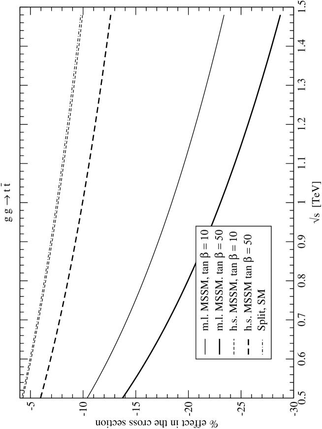
FIG. 1.: Relative percentual effect in the cross section at partonic level for the process $gg\to t\overline{t}$ in various scenarios. Notice that there is no difference between SM and Split in our treatment.

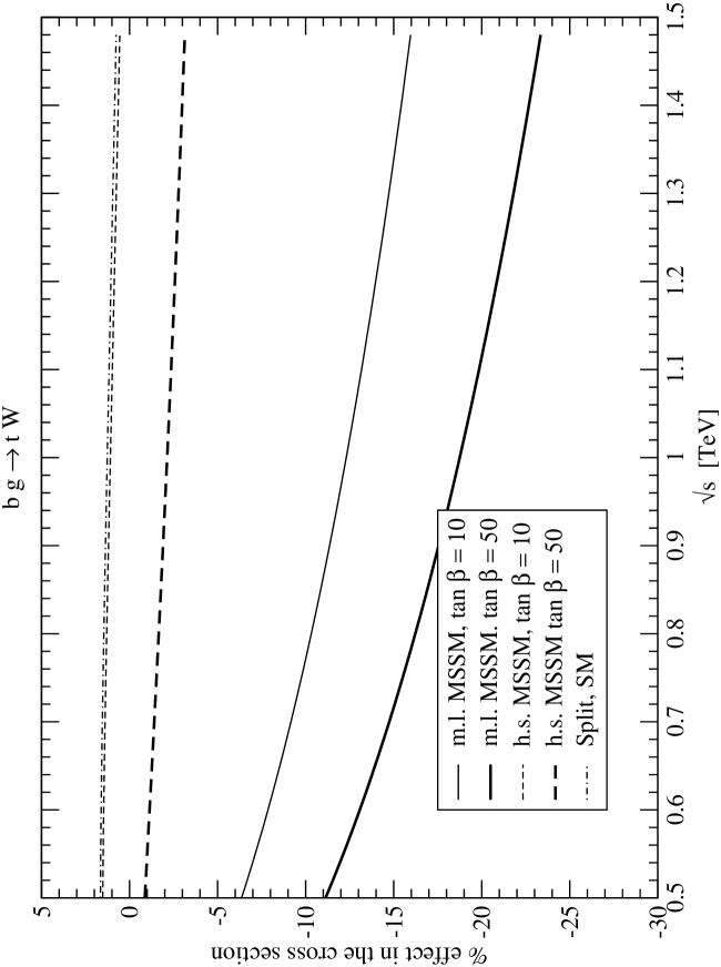
FIG. 2.: Relative percentual effect in the cross section at partonic level for the process $bg\to tW^{-}$ in various scenarios. Notice that there is no difference between SM and Split in our treatment.

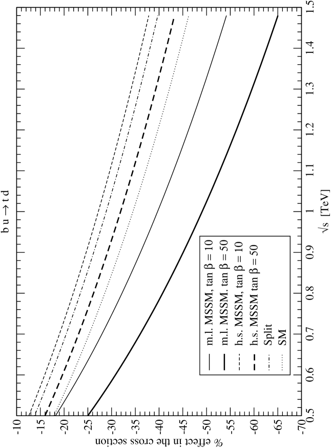
FIG. 3.: Relative percentual effect in the cross section at partonic level for the process $bu\to td$ in various scenarios.

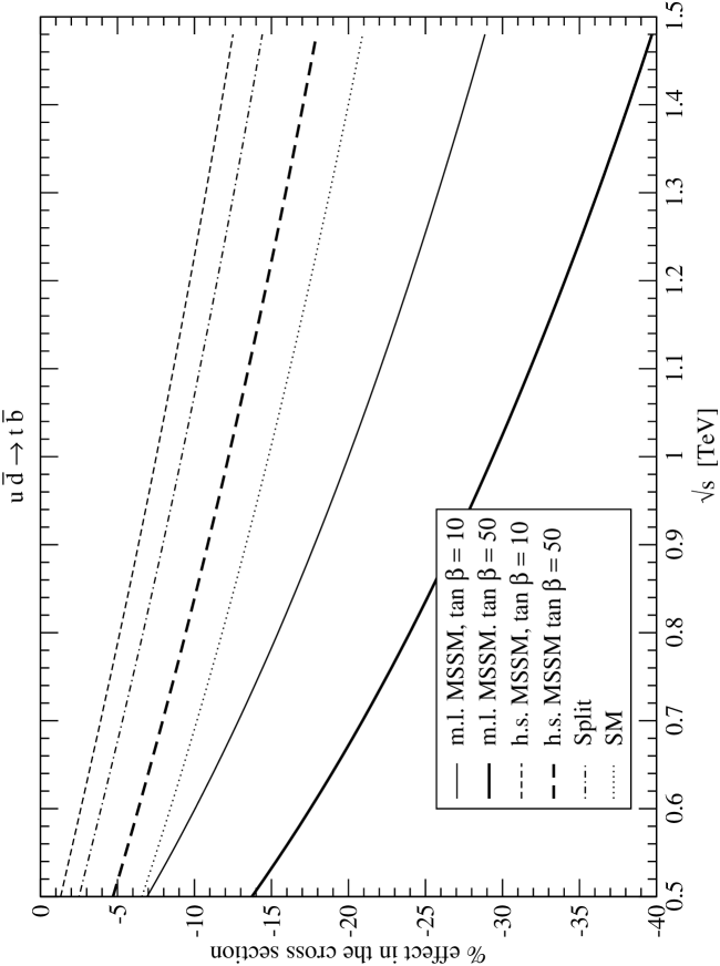
FIG. 4.: Relative percentual effect in the cross section at partonic level for the process $u\overline{d}\to t\overline{b}$ in various scenarios.

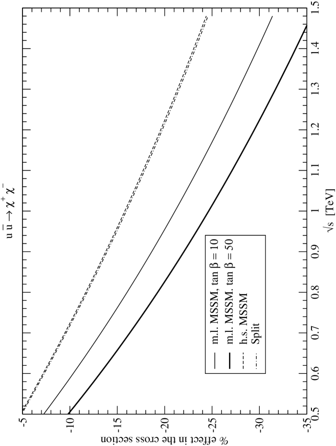
FIG. 5.: Relative percentual effect in the cross section at partonic level for the process $u\overline{u}\to\chi^{+}\chi^{-}$ in various scenarios. Notice that there is no $\tan\beta$ dependence in the model “h.s. MSSM”.

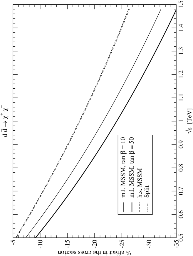
FIG. 6.: Relative percentual effect in the cross section at partonic level for the process $d\overline{d}\to\chi^{+}\chi^{-}$ in various scenarios. Notice that there is no $\tan\beta$ dependence in the model “h.s. MSSM”.

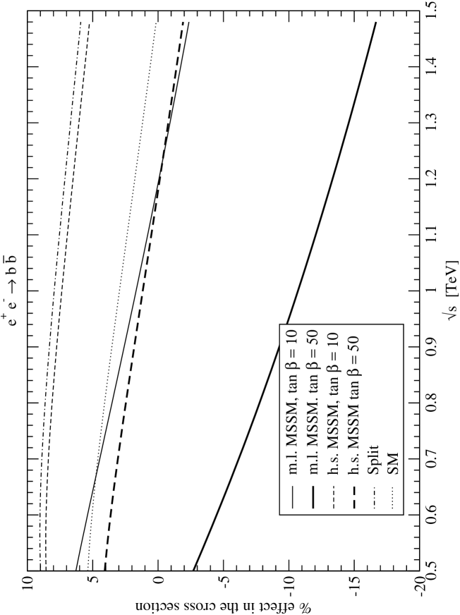
FIG. 7.: Relative percentual effect in the cross section at partonic level for the process $e^{+}e^{-}\to b\overline{b}$ in various scenarios.

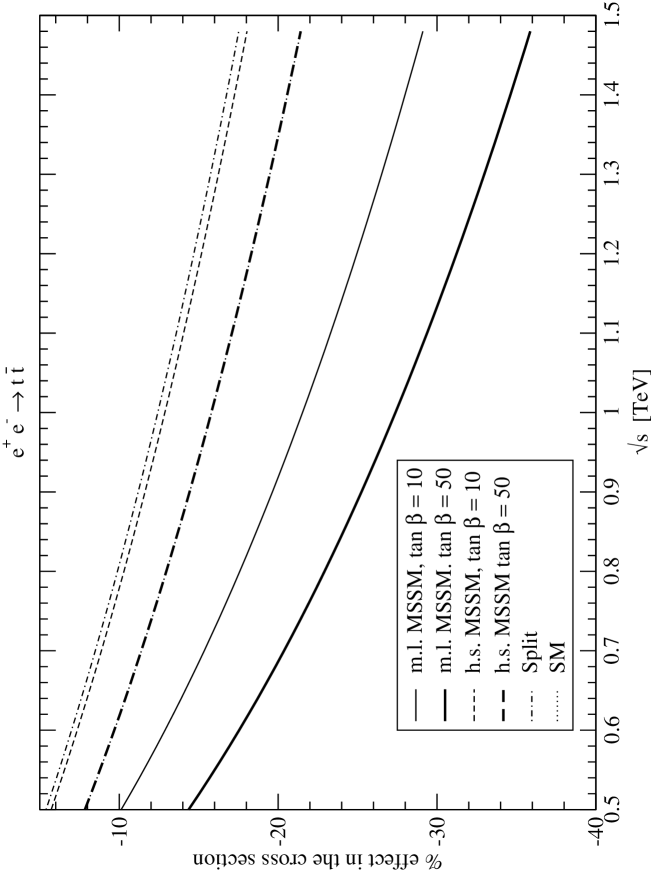
FIG. 8.: Relative percentual effect in the cross section at partonic level for the process $e^{+}e^{-}\to t\overline{t}$ in various scenarios.

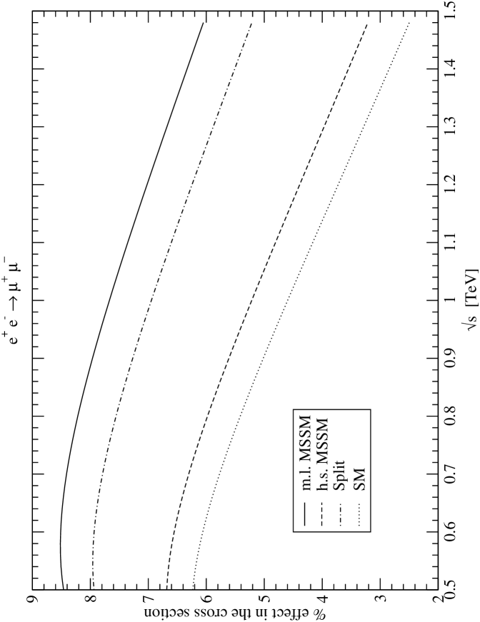
FIG. 9.: Relative percentual effect in the cross section at partonic level for the process $e^{+}e^{-}\to\mu^{+}\mu^{-}$ in various scenarios. There is no $\tan\beta$ dependence both in “m.l. MSSM” and in “h.s. MSSM”.

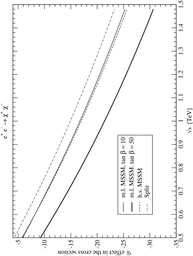
FIG. 10.: Relative percentual effect in the cross section at partonic level for the process $e^{+}e^{-}\to\chi^{+}\chi^{-}$ in various scenarios. Notice that there is no $\tan\beta$ dependence in the model “h.s. MSSM”.

REFERENCES

- [1] N. Arkani-Hamed and S. Dimopoulos, hep-ph/0405159.
- [2] G.F. Giudice and A. Romanino, Nucl. Phys. B699, 65 (2004).
- [3] N. Arkani-Hamed, S. Dimopoulos, G.F. Giudice and A. Romanino, hep-ph/0409232.
- [4] Shou-hua Zhu, Phys. Lett. B 604, 207 (2004).
- [5] W. Kilian, T. Plehn, P.Richarson and E. Schmidt, hep-ph/0408088.
- [6] ”Top quark Physics”, M. Beneke et al, CERN-TH-2000-004, Proc. of the workshop on Standard Model physics (and more) at the LHC; editors G. Altarelli and M. L. Mangano, Geneva 2000, pag. 419.
- [7] M. Beccaria, F.M. Renard and C. Verzegnassi, Phys. Rev. D69, 113004 (2004). M. Beccaria, F.M. Renard and C. Verzegnassi, hep-ph/0410089.
- [8] M. Beccaria, S. Bentvelsen, M. Cobal, F.M. Renard, C. Verzegnassi, hep-ph/0412249.
- [9] M. Beccaria, F. M. Renard and C. Verzegnassi, Phys. Rev. D64, 073008 (2001); M. Beccaria, M. Melles, F. M. Renard and C. Verzegnassi, Phys. Rev. D65, 093007 (2002); M. Beccaria, F.M. Renard and C. Verzegnassi, Phys. Rev. D63, 095010 (2001); M. Beccaria, F.M. Renard and C. Verzegnassi, Phys. Rev. D63, 053013 (2001); M. Beccaria, M. Melles, F.M. Renard, S. Trimarchi, C. Verzegnassi, Int. Jour. Mod. Phys. A18, 5069 (2003).
- [10] N.V. Krasnikov and V.A. Matveev, Phys. Usp. 47, 643 (2004), Usp. Fiz. Nauk. 174, 697 (2004), also available as hep-ph/0309200.
- [11] A. Denner and S. Pozzorini, Eur. Phys.J C18,461(2001); S. Pozzorini, PhD thesis available as hep-ph/0201077.
- [12] J. Rosiek, Phys. Rev. D41, 3464 (1990), hep-ph/9511250 (E).