CERN-2004-005

10 June 2004

Physics Department

hep-ph/0412251

ORGANISATION EUROPÉENNE POUR LA RECHERCHE NUCLÉAIRE

CERN EUROPEAN ORGANIZATION FOR NUCLEAR RESEARCH

PHYSICS AT THE CLIC MULTI-TeV LINEAR COLLIDER

Report of the CLIC Physics Working Group

Editors: M. Battaglia, A. De Roeck, J. Ellis, D. Schulte

CLIC Physics Working Group

E. Accomando (INFN, Torino), A. Aranda (Univ. of Colima), E. Ateser (Kafkas Univ.), C. Balazs (ANL), D. Bardin (JINR, Dubna), T. Barklow (SLAC), M. Battaglia (LBL and UC Berkeley), W. Beenakker (Univ. of Nijmegen), S. Berge (Univ. of Hamburg), G. Blair (Royal Holloway College, Univ. of London), E. Boos (INP, Moscow), F. Boudjema (LAPP, Annecy), H. Braun (CERN), P. Burikham (Univ. of Wisconsin), H. Burkhardt (CERN), M. Cacciari (Univ. Parma), O. Çakır (Univ. of Ankara), A.K. Ciftci (Univ. of Ankara), R. Ciftci (Gazi Univ., Ankara), B. Cox (Manchester Univ.), C. Da Viá (Brunel), A. Datta (Univ. of Florida), S. De Curtis (INFN and Univ. of Florence), A. De Roeck (CERN), M. Diehl (DESY), A. Djouadi (Montpellier), D. Dominici (Univ. of Florence), J. Ellis (CERN), A. Ferrari (Uppsala Univ.), J. Forshaw (Manchester Univ.), A. Frey (CERN), G. Giudice (CERN), R. Godbole (Bangalore), M. Gruwe (CERN), G. Guignard (CERN), T. Han (Univ. of Wisconsin), S. Heinemeyer (CERN), C. Heusch (UC Santa Cruz), J. Hewett (SLAC), S. Jadach (INP, Krakow), P. Jarron (CERN), C. Kenney (MBC, USA), Z. Kırca (Osmangazi Univ.), M. Klasen (Univ. of Hamburg), K. Kong (Univ. of Florida), M. Krämer (Univ. of Edinburgh), S. Kraml (HEPHY Vienna and CERN), G. Landsberg (Brown Univ.), J. Lorenzo Diaz-Cruz (BUAP, Puebla), K. Matchev (Univ. of Florida), G. Moortgat-Pick (Univ. of Durham), M. Mühlleitner (PSI, Villigen), O. Nachtmann (Univ. of Heidelberg), F. Nagel (Univ. of Heidelberg), K. Olive (Univ. of Minnesota), G. Pancheri (INFN, Frascati), L. Pape (CERN), S. Parker (Univ. of Hawaii), M. Piccolo (LNF, Frascati), W. Porod (Univ. of Zurich), E. Recepoglu (Univ. of Ankara), P. Richardson (Univ. of Durham), T. Riemann (DESY-Zeuthen), T. Rizzo (SLAC), M. Ronan (LBL, Berkeley), C. Royon (CEA, Saclay), L. Salmi (HIP, Helsinki), D. Schulte (CERN), R. Settles (MPI, Munich), T. Sjostrand (Lund Univ.), M. Spira (PSI, Villigen), S. Sultansoy (Gazi Univ., Ankara and IP Baku), V. Telnov (Novosibirsk, IYF), D. Treille (CERN), M. Velasco (Northwestern Univ.), C. Verzegnassi (Univ. of Trieste), G. Weiglein (Univ. of Durham), J. Weng (CERN, Univ. of Karlsruhe), T. Wengler (CERN), A. Werthenbach (CERN), G. Wilson (Univ. of Kansas), I. Wilson (CERN), F. Zimmermann (CERN)

CERN Scientific Information Service–1000–June 2004

Abstract

This report summarizes a study of the physics potential of the CLIC $e^{+}e^{-}$ linear collider operating at centre-of-mass energies from 1 TeV to 5 TeV with luminosity of the order of 10³⁵ cm^-2 s^-1. First, the CLIC collider complex is surveyed, with emphasis on aspects related to its physics capabilities, particularly the luminosity and energy, and also possible polarization, $\gamma\gamma$ and $e^{-}e^{-}$ collisions. The next CLIC Test facility, CTF3, and its R&D programme are also reviewed. We then discuss aspects of experimentation at CLIC, including backgrounds and experimental conditions, and present a conceptual detector design used in the physics analyses, most of which use the nominal CLIC centre-of-mass energy of 3 TeV. CLIC contributions to Higgs physics could include completing the profile of a light Higgs boson by measuring rare decays and reconstructing the Higgs potential, or discovering one or more heavy Higgs bosons, or probing CP violation in the Higgs sector. Turning to physics beyond the Standard Model, CLIC might be able to complete the supersymmetric spectrum and make more precise measurements of sparticles detected previously at the LHC or a lower-energy linear $e^{+}e^{-}$ collider: $\gamma\gamma$ collisions and polarization would be particularly useful for these tasks. CLIC would also have unique capabilities for probing other possible extensions of the Standard Model, such as theories with extra dimensions or new vector resonances, new contact interactions and models with strong $WW$ scattering at high energies. In all the scenarios we have studied, CLIC would provide significant fundamental physics information beyond that available from the LHC and a lower-energy linear $e^{+}e^{-}$ collider, as a result of its unique combination of high energy and experimental precision.

Chapter 1 INTRODUCTION

The energy range up to 100 GeV has been explored by the hadron–hadron colliders at CERN and Fermilab, by the LEP $e^{+}e^{-}$ collider and the SLC, and by the $ep$ collider HERA. The next energy frontier is the range up to 1 TeV, which will first be explored by the LHC. Just as $e^{+}e^{-}$ colliders provided an essential complement to hadron–hadron colliders in the 100 GeV energy range, establishing beyond doubt the validity of the Standard Model, so we expect that higher-energy $e^{+}e^{-}$ colliders will be needed to help unravel the TeV physics, to be unveiled by the LHC. They provide very clean experimental environments and democratic production of all particles within the accessible energy range, including those with only electroweak interactions. These considerations motivate several projects for $e^{+}e^{-}$ colliders in the TeV energy range, such as TESLA, the NLC and JLC. We assume that at least one of these projects will start up during the operation of the LHC. However, we do not expect that the full scope of TeV-scale physics will then be exhausted, and we therefore believe that a higher-energy $e^{+}e^{-}$ collider will be needed.

The best candidate for new physics at the TeV scale is that associated with generating masses for elementary particles. This is expected to involve a Higgs boson, or something to replace it. The precision electroweak data from LEP and elsewhere rule out many alternatives to the single elementary Higgs boson predicted by the Standard Model, and suggest that it should weigh $\lappeq$ 200 GeV. A single elementary Higgs boson is not thought to be sufficient by itself to explain the variety of the different mass scales in physics. Many theories beyond the Standard Model, such as those postulating supersymmetry, extra dimensions or new strong interactions, predict the appearance of non-trivial new dynamics at the TeV scale.

For example, supersymmetry predicts that every particle in the Standard Model should be accompanied by a supersymmetric partner weighing $\lappeq$ 1 TeV. Alternatively, theories with extra spatial dimensions predict the appearance of new particle excitations or other structural phenomena at the TeV scale. Finally, alternatives to an elementary Higgs boson, such as new strong interactions, also predict many composite resonances and other effects observable at the TeV energy scale.

Whilst there is no direct evidence, there are various indirect experimental hints that there is indeed new dynamics at the TeV scale. One is the above-mentioned agreement of precision electroweak data with the Standard Model, if there is a relatively light Higgs boson. Another is the agreement of the gauge couplings measured at LEP and elsewhere with the predictions of simple grand unified theories, if there is a threshold for new physics at the TeV scale, such as supersymmetry. Another hint may be provided by the apparent dominance of dark matter in the Universe, which may well consist of massive, weakly-interacting particles, in which case they should weigh $\lappeq$ 1 TeV. Finally, we note that there may be a discrepancy between the measurement of the anomalous magnetic moment of the muon and the prediction of the Standard Model, which could only be explained by new dynamics at the TeV scale.

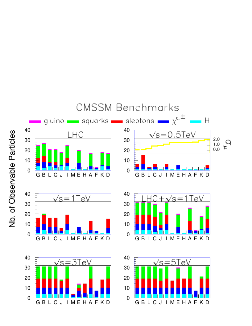
Figure 1.1: Bar charts of the numbers of different sparticle species observable in a number of benchmark supersymmetric scenarios at different colliders, including the LHC and linear $e^{+}e^{-}$ colliders with various centre-of-mass energies. The benchmark scenarios are ordered by their consistency with the most recent BNL measurement of $g_{\mu}-2$ and are compatible with the WMAP data on cold dark matter density. We see that there are some scenarios where the LHC discovers only the lightest neutral supersymmetric Higgs boson. Lower-energy linear $e^{+}e^{-}$ colliders largely complement the LHC by discovering or measuring better the lighter electroweakly-interacting sparticles. Detailed measurements of the squarks would, in many cases, be possible only at CLIC.

We expect that the clean experimental conditions at a TeV-scale linear $e^{+}e^{-}$ collider will enable many detailed measurements of this new dynamics to be made. However, we also expect some aspects of TeV-scale physics to require further study using a higher-energy $e^{+}e^{-}$ collider. For example, if there is a light Higgs boson, its properties will have been studied at the LHC and the first $e^{+}e^{-}$ collider, but one would wish to verify the mechanism of electroweak symmetry breaking by measuring the Higgs self-coupling associated with its effective potential, which would be done better at a higher-energy $e^{+}e^{-}$ collider. On the other hand, if the Higgs boson is relatively heavy, measurements of its properties at the LHC or a lower-energy $e^{+}e^{-}$ collider will quite possibly have been incomplete. As another example, if Nature has chosen supersymmetry, it is quite likely that the LHC and the TeV-scale $e^{+}e^{-}$ collider will not have observed the complete sparticle spectrum, as seen in Fig. 1.1.

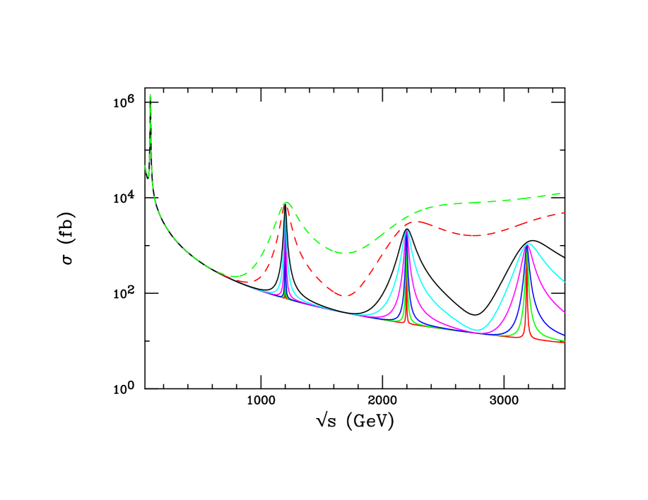
Figure 1.2: An example of the dilepton spectrum that might be observed at the LHC in some scenario for extra dimensions, including Kaluza–Klein excitations of the photon and $Z$ and their interferences.

Moreover, in many cases detailed measurements at a higher-energy $e^{+}e^{-}$ collider would be needed to complement previous exploratory observations, e.g. of squark masses and mixing, or of heavier charginos and neutralinos. Analogous examples of the possible incompleteness of measurements at the LHC and the TeV-scale $e^{+}e^{-}$ collider can be given in other scenarios for new physics, such as extra dimensions, as discussed in later chapters of this report. Certainly a multi-TeV linear $e^{+}e^{-}$ collider would be able to distinguish smaller extra dimensions than a sub-TeV machine. Even if prior machines do uncover extra dimensions, it would, for example, be fascinating to study in detail at CLIC a Kaluza–Klein excitation of the $Z$ boson that might have been discovered at the LHC, as seen in Fig. 1.2.

For all the above reasons, we think that further progress in particle physics will necessitate clean experiments at multi-TeV energies, such as would be possible at a higher-energy $e^{+}e^{-}$ collider like CLIC. This would, in particular, be the logical next step in CERN’s vocation to study physics at the high-energy frontier. CERN and collaborating institutes have already made significant progress towards demonstrating the feasibility of this accelerator concept, whilst other projects for reaching multi-TeV energies, such as a $\mu^{+}\mu^{-}$ collider or a very large hadron collider, seem to be more distant prospects.

Some exploratory studies of CLIC physics have already been made, but the close integration of experiments at linear $e^{+}e^{-}$ colliders with the accelerator, particularly in the final-focus region, now mandate a more detailed study, as described in this report.

Chapter 2 summarizes the design of the CLIC accelerator, including the overall design concept, its general parameters such as energy and luminosity, the collision energy spread, the prospects for obtaining polarized beams, and the option for a $\gamma\gamma$ collider. A crucial step has recently been demonstrated at the second CLIC test facility, namely the attainment of an accelerating gradient in excess of 150 MeV/m. Chapter 3 discusses experimental aspects, such as the levels of experimental backgrounds expected, the specification of a baseline detector, the luminosity measurement, and the simulation tools available for experimental studies.

Chapter 4 is devoted to Higgs physics, including the prospects for measuring the triple-Higgs coupling for a relatively light Higgs boson, heavy-Higgs studies, the possibility of observing CP violation in the heavy-Higgs sector of the minimal supersymmetric extension of the Standard Model (MSSM), and possible Higgs studies with a $\gamma\gamma$ collider.

Chapter 5 reviews possible studies of supersymmetry at CLIC, with particular attention to certain benchmark MSSM scenarios where we demonstrate their complementarity with studies at the LHC and a lower-energy $e^{+}e^{-}$ collider. We discuss in particular possible precision measurements of sleptons, squarks, heavier charginos and neutralinos, and the possibility of gluino production in $\gamma\gamma$ collisions.

Other scenarios for new physics are presented in Chapter 6, including direct and indirect observations of extra dimensions, black-hole production, non-commutative theories, etc. Chapter 7 summarizes QCD studies that would be possible at CLIC, in both $e^{+}e^{-}$ and $\gamma\gamma$ collisions.

Finally, Chapter 8 summarizes the conclusions of this study of the physics accessible with CLIC.

Chapter 2 ACCELERATOR ISSUES AND PARAMETERS

2.1 Overview of the CLIC Complex

The CLIC (Compact Linear Collider) study aims at a multi-TeV, high-luminosity $e^{+}e^{-}$ linear collider. In order to reach high energies with a linear collider, a cost-effective technology is of prime importance. In conventional linear accelerators, the RF power used to accelerate the main beam is generated by klystrons. To achieve multi-TeV energies, high accelerating gradients are necessary to limit the lengths of the two main linacs and hence the cost. Such high gradients are easier to achieve at higher RF frequencies since, for a given gradient, the peak power in the accelerating structure is smaller than at low frequencies. For this reason, a frequency of 30 GHz has been chosen for CLIC to attain a gradient of 150 MV/m. However, the production of highly efficient klystrons is very difficult at high frequency. Even in the X-band at 11.5 GHz, a very ambitious programme has been necessary at SLAC and KEK to develop prototypes that come close to the required performance. At even higher frequencies, the difficulties of building efficient high-power klystrons are significantly larger. Instead, the CLIC study is based on the two-beam accelerator scheme. The RF power is extracted from a low-energy, high-current drive beam, which is decelerated in power extraction and transfer structures of low impedance. This power is then directly transferred into the high-impedance structures of the main linac and used to accelerate the high-energy, low-current main beam, which is later brought into collision. The two-beam approach offers a solution that avoids the use of a large number of active RF elements, e.g. klystrons or modulators, in the main linac. This potentially eliminates the need for a second tunnel.

In the CLIC scheme, the drive beam is created and accelerated at low frequency (0.937 GHz) where efficient klystrons can be realized more easily. The frequency and intensity of the beam is then increased in the chain of a delay loop and two combiner rings. This drive-beam generation system can be installed at a central site, thus allowing easy access and replacement of the active RF elements.

The CLIC design parameters have been optimized for a nominal centre-of-mass energy $\sqrt{s}$ = 3 TeV with a luminosity of about 10³⁵ cm^-2s^-1 [1], but the CLIC concept allows its construction to be staged without major modifications (see Fig. 2.1). The possible implementation of a lower-energy phase for physics would depend on the physics requirements at the time of construction. In principle, a first CLIC stage could cover centre-of-mass energies between $\sim$ 0.1 and 0.5 TeV with a luminosity of $\mathcal{L}$ = 10³³–10³⁴ cm^-2s^-1, providing an interesting physics overlap with the LHC. This stage could then be extended first to 1 TeV, with $\mathcal{L}$ above 10³⁴ cm^-2s^-1, and then to multi-TeV operation, with $e^{+}e^{-}$ collisions at 3 TeV, which should break new physics ground. A final stage might reach a collision energy of 5 TeV or more.

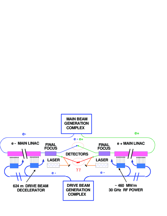
Figure 2.1: The schematics of the overall layout of the CLIC complex

The sketch of Fig. 2.1 gives an overall layout of the complex with the linear decelerator units running parallel to the main beam [2]. Each unit is 625 m long and decelerates a low-energy, high-intensity $e^{-}$ beam, the drive-beam, which provides the RF power for each corresponding unit of the main linac through energy-extracting RF structures. Hence, there are no active elements in the main tunnel. With a gradient of 150 MV/m, the main beam is accelerated by $\sim$ 70 GeV in each unit. Consequently, the natural lowest value and step size of the colliding beam energy in the centre of mass ($\sqrt{s}$) is $\sim$ 140 GeV, though both can be tuned by adjusting the drive-beam and decelerator. The nominal energy of 3 TeV requires 2 $\times$ 22 units, for a total two-linac length of $\sim$ 28 km. Each unit contains 500 power-extraction transfer structures (PETSs) feeding 1000 accelerating structures.

The two-beam acceleration method of CLIC ensures that the design remains essentially independent of the final energy for all the major subsystems, such as the main beam injectors, the damping rings, the drive-beam generators, the RF power source, the main-linac and drive-beam decelerator units, as well as the beam delivery systems (BDSs). The CLIC modularity is made easier by the fact that the complexes for the generation of all the beams and the interaction point (IP) are located at a central position, where all power sources are also concentrated. The main tunnel houses both linacs, the various beam transfer lines and, in its centre, the BDSs.

This chapter summarizes the CLIC two-beam study and discusses the interplay between the achievable energy and luminosity and the design of the various accelerator system components, with emphasis on the features most relevant to the CLIC physics performance. These systems are the focus of a continuing research and development programme, in particular for the high-gradient structures, the damping rings, the vibration stabilization systems, and the beam delivery section. The main-beam and the drive-beam parameters are summarized in Table 2.1, for the nominal energy of 3 TeV as well as for 500 GeV, as an example for lower energies.

Table 2.1: Main CLIC machine parameters

Collision energy $\sqrt{s}$    (TeV)	0.5	3.0
Design luminosity $\cal{L}$ (1035 cm-2s-1)	0.2	0.8
Linac repetition frequency (Hz)	200	100
No. of ptcs./bunch $N$ (1010)	0.4	0.4
No. of bunches/pulse $n_{b}$	154	154
Bunch separation (ns)	0.67	0.67
Bunch length ($\mu$m)	35	35
Normalized emittance $\gamma\epsilon^{*}_{x}$/$\gamma\epsilon^{*}_{y}$ (m$\cdot$rad $\times$ 10-6)	2.0/0.01	0.68/0.01
Beam size at collision $\sigma^{*}_{x}$/$\sigma^{*}_{y}$/$\sigma^{*}_{z}$ (nm/nm/$\mu$m))	202/12/35	60/0.7/35
Energy spread $\Delta E/E$ (%)	0.25	0.35
Crossing angle (mrad)	20	20
Beamstrahlung $\delta_{B}$ (%)	4.4	21
Beam power/beam (MW)	4.9	14.8
Gradient unloaded/loaded (MV/m)	150	150
Two-linac length (km)	5.0	28.0
Beam delivery length (km)	5.2	5.2
Final focus length (km)	1.1	1.1
Total site length (km)	10.2	33.2
Total AC power (MW)	175	410

2.2 CLIC Energy and RF Technology Choice

Linear, single-pass colliders are currently the most advanced concepts for particle accelerators capable of reaching multi-TeV energies in lepton collisions. At these energies, the choice of technology may be narrowed down to high-frequency, normal-conducting cavities for the reasons discussed above. Superconducting linac technology, such as that proposed for the lower-energy TESLA collider, is limited to accelerating gradients of about 50 MV/m. At this value, the critical magnetic field strength for superconductivity is reached on the cavity walls. This limit is fundamental and cannot be overcome, at least in the present theoretical understanding of superconductivity. Using normal conducting linear accelerator technology, as employed for the SLC and now proposed for the NLC/JLC projects, the achievable accelerating gradients are considerably higher, in principle. Gradients of 65 MV/m are now routinely achieved with NLC/JLC test structures in the X band at 11.5 GHz over long running periods.

In principle, higher RF frequencies facilitate higher field strength. Furthermore in the high beamstrahlung regime the luminosity increases with the RF frequency and is independent of the gradient. Recent results at dedicated test facilities have shown, however, that above $\simeq$ 10 GHz the cavity geometry, material and surface preparation become the predominant factors, determining the achievable accelerating fields [3]. The choice of frequency for normal conducting linacs is therefore based on an optimization of other aspects, such as beam dynamics, technical feasibility, power consumption, and investment costs.

The energy needed to establish a given accelerating field $E$ over a given length scales with $\nu^{2}$, which can readily be understood from the scaling of cavity dimensions with the frequency $\nu$. The time scale for the dissipation of this energy by resistive losses on the cavity walls in conjunction with the skin effect scales like $\nu^{-3/2}$. Hence, the instantaneous power per unit length to maintain a certain field strength scales as $\nu^{-1/2}$, favouring higher frequencies. However, the small cavity dimensions at high frequency lead to strong beam-induced transverse wakefields, generating transverse instabilities. These limit the number of particles that can be stored in a single bunch and hence the luminosity. This effect can be offset by choosing a shorter bunch length $\sigma_{z}$ at higher frequency, which increases the luminosity for multi-TeV collisions. To take advantage of from this effect, the horizontal beam size at the interaction point has to be decreased with increasing frequency. This beam size has, however, a lower limit due to the performance of damping rings and beam-delivery systems [4].

Considering these aspects together, it turns out that for an accelerating field of 150 MV/m the overall cost as a function of frequency has a rather flat minimum between 20 GHz and 30 GHz. For lower frequencies the costs to supply the pulsed RF energy become prohibitive and for higher frequencies the reduced bunch charge precludes sufficient luminosity with present damping ring and beam-delivery systems [5].

The RF power needed to establish an accelerating field of 150 MV/m is about 100–200 MW/m at 30 GHz, with the precise value depending on the details of the cavity geometry. While such power can only by supplied over short pulses, it would be more favourable from the RF power-source point of view to supply a given amount of pulse energy in a longer pulse of lower power. To reconcile these conflicting requirements, different RF pulse compression schemes have been developed. In the case of NLC/JLC, the compression is performed by intermediate storage of long RF pulses in low loss waveguides. In the CLIC design, the compression is achieved by accelerating a long drive beam pulse in a low frequency (937 MHz) accelerator. This long pulse is wound up in a combiner ring using a sophisticated injection scheme based on RF dipoles. This scheme achieves multiplication of the bunch repetition frequency and pulse compression simultaneously.

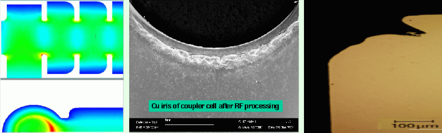
Figure 2.2: Macro-photographs of the input coupler of a 30 GHz RF copper structure, showing the erosion damage subsequent to breakdown in RF tests

The limiting factors to the achievable accelerating gradient are the RF breakdown in the cavities and the related erosion of the cavity surfaces. Erosion effects due to breakdown were observed in early tests of a CLIC prototype structure, whose damaged iris is shown in Fig. 2.2. The physics of these breakdowns is currently not precisely known. It is generally believed that field emission from the cavity walls triggering a runaway plasma formation is the process responsible for it. Recent experiments in the CLIC Test Facility 2 (CTF2) indicate that these effects can be overcome, in normal operating conditions, by replacing the copper with either molybdenum or tungsten as material for the structure irises. Figure 2.3 summarizes the results obtained with test structures adopting this new configuration. The feasibility of achieving gradients up to 193 MV/m has thus been demonstrated [6] in CTF2 for short RF pulses. Tests with pulses of nominal length will become possible in the CLIC Test Facility 3 (CTF 3).

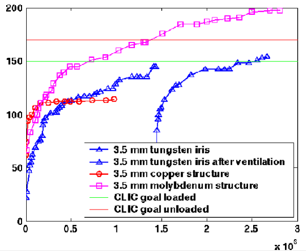
Figure 2.3: Accelerating gradients obtained with 30 GHz structures of different designs. The gradient measured in the first cell of the structure is shown as a function of the number of applied RF pulses.

Pulsed surface heating represents another potentially severe limitation. Although the present CLIC RF structure design attempts to minimize this effect, a temperature rise still beyond that sustained in present linacs is expected. A full understanding of its impact on the operation of the cavities will become possible once CTF3 provides 30 GHz RF pulses of the designed length and amplitude.

2.3 CLIC Luminosity

The luminosity ${\cal L}$ in a linear collider can be expressed as a function of the effective transverse beam sizes $\sigma_{x,y}$ at the interaction point (IP), the bunch population $N$, the number of bunches $n_{b}$ per beam pulse and the number of pulses per second $f_{r}$:

$${\cal L}=H_{D}\frac{N^{2}}{4\pi\sigma_{x}\sigma_{y}}n_{b}f_{r}\,.$$ (2.1)

Here, the luminosity enhancement factor $H_{D}$, which is usually in the range of 1–2, is due to the beam–beam interaction, which focuses the $e^{+}e^{-}$ beams during collision. The equation can be expressed as a function of the power consumption $P$ of the collider and of the total power to beam power efficiency $\eta$, obtaining:

$${\cal L}\propto H_{D}\frac{N}{\sigma_{x}}\frac{1}{\sigma_{y}}\eta P\,.$$ (2.2)

The different parameters are not independent and the dependences can be quite complex. However, three main fundamental limitations arise from the factors $N/\sigma_{x}$, $\sigma_{y}$ and $\eta$, if the other parameters are kept fixed.

• The optimum ratio $N/\sigma_{x}$ is determined by the beam–beam interaction. At large $N/\sigma_{x}$ the total luminosity is highest, but the colliding particles strongly emit beamstrahlung during the collision. Hence the luminosity spectrum will be degraded and the backgrounds higher.

• The value of $\sigma_{y}$ is, in the case of CLIC, mainly limited by the difficulty of creating such a small beam size and by the difficulty of keeping two small beams in collision. The achievable $\sigma_{y}$ depends on the bunch charge $N$.

• The efficiency of the beam acceleration $\eta$ mainly depends on the RF technology chosen for the main linac and on the beam current, e.g. larger $N$ leads to better efficiency.

The above parameters are strongly coupled. An important example for a coupling parameter is the bunch length $\sigma_{z}$. In a given main linac the bunch length is a function of the bunch charge, larger $N$ requiring larger $\sigma_{z}$. In turn, the optimum ratio $N/\sigma_{x}$ is a function of $\sigma_{z}$. The achievable $\sigma_{y}$ also depends on $N$, since larger $N$ and larger $\sigma_{z}$ lead to larger $\sigma_{y}$.

An additional limitation arises from the damping ring and the beam delivery system.

• For the nominal CLIC parameters, a lower limit $\sigma_{x}\geq$ 60 nm is currently found. The damping ring and the beam delivery system contribute equally to this limit. It remains to be investigated if this limit is fundamental.

In the following the limitations for the three main factors that determine the luminosity are presented. The trade-off between luminosity and beamstrahlung at the interaction point is discussed first. Then the issues related to achieving the small needed $\sigma_{y}$ are detailed, with emphasis on the resulting luminosity.

2.3.1 Horizontal Beam Size and Bunch Charge

A fundamental lower limit to the ratio of bunch charge and horizontal beam size at the IP arises from the strong beam–beam interaction. Because of this effect, the beams are focused during the collision. While increasing the luminosity ${\cal L}$, this gives rise to the emission of beamstrahlung, with each beam particle typically emitting $O(1)$ photon. The beamstrahlung alters the beam particles’ energies, so that particles can collide at energies different from nominal and a wide luminosity spectrum is delivered. In most physics investigations, only some fraction of the luminosity ${\cal L}_{1}$ close to the nominal centre-of-mass energy is of interest.

If one keeps the other parameters constant, the beamstrahlung depends almost completely on the ratio $N/\sigma_{x}$. Decreasing $\sigma_{x}$ or increasing $N$ increases the total luminosity, but also increases the beamstrahlung. Consequently the fraction of luminosity close to the nominal energy ${\cal L}_{1}/{\cal L}$ decreases. For otherwise fixed parameters an optimum $\sigma_{x}$ exists, which maximizes ${\cal L}_{1}$, see Fig. 2.4. However, the optimum $\sigma_{x}$ and the maximum luminosity ${\cal L}_{1}$ depend on these other parameters. As can be seen in the figure, the use of a shorter bunch allows one to use a smaller horizontal beam size and yields a higher luminosity even for the same transverse size.

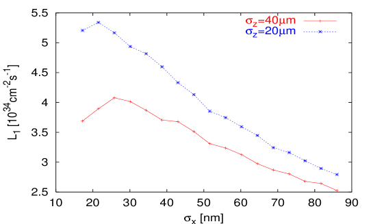
Figure 2.4: The high-energy luminosity ${\cal L}_{1}$ as a function of the horizontal beam size for two different bunch lengths and nominal bunch charge. In both cases there exists a clear optimum. For the shorter bunch length the total peak luminosity is higher since the beamstrahlung is more suppressed.

However, it is not only the wish to maximize ${\cal L}_{1}$ that can lead to a lower limit on $\sigma_{x}$. One may also require a certain quality of the luminosity spectrum (e.g. for threshold studies) or certain background conditions: at smaller $\sigma_{x}$ the background levels will be higher.

With the current damping ring and BDS designs it is found that one cannot achieve horizontal beam sizes below about $\sigma_{x}\geq$ 60 nm. If this limit is fundamental, it will make it impossible to achieve the optimum $N/\sigma_{x}$ for small bunch charges, with the consequences discussed in Section 2.3.3

2.3.2 Vertical Beam Size

In order to achieve a small vertical beam size at the IP, the vertical phase space occupied by the beam—the vertical emittance $\epsilon_{y}$—must be small. The total effective beam size at the IP can be expressed in a simplified way as a function of the total emittance and the focal strength of the final-focus system (described by $\beta_{y}$):

$$\sigma_{y,{\rm eff}}\propto\sqrt{\beta_{y}\left(\epsilon_{y,{\rm DR}}+\epsilon_{y,{\rm BC}}+\epsilon_{y,{\rm linac}}+\epsilon_{y,{\rm BDS}}+\epsilon_{y,{\rm jitter}}\right)}\,.$$ (2.3)

Consequently a number of challenges have to be met to achieve a small vertical beam size.

• First, a beam with a small emittance $\epsilon_{y,{\rm DR}}$ must be created in the damping ring. The target for CLIC is $\epsilon_{y,{\rm DR}}\leq$ 3 nm.

• This beam needs to be longitudinally compressed and transported to the main linac with a small emittance growth $\epsilon_{y,{\rm BC}}$. The target is $\epsilon_{y,{\rm BC}}\leq$ 2 nm.

• The emittance growth during the acceleration in the main linac $\epsilon_{{\rm linac}}$ has to be kept small. The target is $\epsilon_{y,{\rm linac}}\leq$ 10 nm.

• In the BDS the beam tails are scraped off and the beam is focused to a very small spot size. This system must also lead to a small emittance growth $\epsilon_{{\rm BDS}}$ and at the same time achieve strong focusing, i.e. a small vertical beta-function $\beta_{y}$. The target is $\epsilon_{y,{\rm BDS}}\leq$ 10 nm for the nominal $\beta_{y}$ = 70 $\mu$m.

• The beams need to collide. Dynamic effects in the whole accelerator lead to a continuous motion of the beam trajectory, and this motion can be described by a growth of the multi-pulse emittance $\epsilon_{y,{\rm jitter}}$. This growth should be much smaller than the other contributions.

It is obvious that all the emittance contributions must be minimized to achieve a small spot size and that further optimization of one value becomes useless if the sum is dominated by some other contribution. The different contributions are not independent, but for the sake of simplicity, they are discussed separately in the following. For each subsystem a design must first be developed, which in principle can achieve the required performance; then the consequences of imperfect realizations of this design must be considered and finally the effects of dynamic imperfections.

2.3.2.1 Damping ring emittance

The vertical emittance of the beam is large at production. Hence, it needs to be reduced in a damping ring. The design value for the vertical emittance after the damping ring is $\epsilon_{y,{\rm DR}}$ = 3 nm. The possibility to achieve this is currently under investigation. Simulations of different possible layouts of the ring have so far not reached values better than $\epsilon_{y,{\rm DR}}$ = 9 nm [7]. In addition, not all effects in the ring have been studied yet, in particular the imperfections. However, it is hoped that the design can be improved by a further optimization that takes into account all the limiting physics effects at the design stage.

2.3.2.2 Bunch compressor emittance growth

A design for the bunch compressor exists, but its performance has not been completely evaluated [8]. In particular, the simulation of the emittance growth due to coherent synchrotron radiation and imperfections remains to be done. However, preliminary studies of the coherent synchrotron radiation indicate that they remain acceptable [9].

2.3.2.3 Main linac emittance growth

The preservation of the emittance in the main linac is one of the major challenges in a linear collider design. This is due to a large extent to the so-called wakefields that the beam experiences when passing the accelerating structures. The size of these wakefields is strongly dependent on the chosen accelerating technology and frequency. The design of the main linac has now reached a relatively mature state and some significant work has already been done to estimate and minimize the effect of imperfections, which is the main issue.

Structure offsets from the nominal beam line induce a transverse electric field, the wakefield, which induces a transverse kick on the beam. This effect can be large, especially in a high-frequency linac. The emittance growth due to imperfections can be tackled with different countermeasures.

• First, the main linac lattice is designed to reduce the sensitivity to such imperfections.

• Second, a sophisticated prealignment system using wires, lasers and hydrostatic levelling devices is foreseen to position the elements in CLIC with small errors to reduce the imperfections.

• Third, beam-based alignment will be used. Small remaining imperfections are detected using the beam itself, and their effect on the beam is corrected. Simulations predict that, after application of these procedures, most of the remaining emittance growth is due to the wakefields in the RF structures of the main linac[10].

• The accelerating structures are mounted on movable girders and each of them incorporates a beam position monitor. This allows one to correct their position with respect to the beam by direct observation and minimization of the beam offset.

• Finally, so-called emittance tuning bumps are used. A few structures are moved in order to minimize the emittance at the end of the linac. This globally compensates the mean beam offset, which remains because of imperfect measurement of the beam position in each structure.

The final emittance growth after these steps is about 1.5 nm and thus significantly smaller than the target.

The dependence of the emittance growth on the bunch charge and structure can be seen in Fig. 2.5. The structure with an iris radius $a$ = 2 mm corresponds to the reference design of the accelerating structure. As can be seen, the structures with larger values of $a$ (the radius of the iris) allow larger bunch charges. However, it is more difficult to achieve the required gradient in them.

Figure 2.5: The emittance growth $\epsilon_{{\rm linac}}$ in the main linac as a function of the bunch charge $N$ for different structures

2.3.2.4 Beam delivery system emittance growth

In the final focus system (FFS) the beam is strongly focused, and consequently the system has a tendency to be very chromatic. Since the beam has an energy spread, one needs to reduce the chromaticity by a delicate system of cancelling magnets; but some residual effect remains. Another problem arises from the emission of synchrotron radiation in the magnets. While the resulting stochastic energy change of the particles is smaller than the energy difference between incoming particles, it can destroy the delicate cancellation between different magnets. Because of these two effects there is a lower limit to the achievable $\beta_{y}$, and $\epsilon_{y,{\rm BDS}}$ is not zero even for an error-free lattice. The current design of the FFS achieves an effective vertical beam size of $\sigma_{y}\approx$ 0.7 nm [11], whereas the rms beam size is much larger. If the two above-mentioned problems were not present, the size would be $\sigma_{y}$ = 0.5 nm. The effect can be understood as a doubling of the vertical emittance that enters the BDS, corresponding to an emittance growth of $\epsilon_{y,{\rm BDS}}$ = 10 nm, though the actual dependence is more complicated. This performance is better than the original target of 1 nm. It compensates approximately the fact that the effective horizontal beam size is larger than the target.

2.3.2.5 Dynamic imperfections

Dynamic effects finally limit $\sigma_{y,{\rm eff}}$ in two ways. First, they make it more difficult to achieve a small emittance in all the different subsystems. Second, they let the beams miss each other at the IP; this does not change the size of a single bunch but the phase space occupied by a number of consecutive bunch trains, as summarized in Eq. (2.3) by $\epsilon_{y,{\rm jitter}}$. A number of effects can lead to transverse jitter. Potentially important sources are motion of the ground, vibration of quadrupoles in the beam line due to cooling water, vibrations of the accelerating structures, and a number of other effects. Also very important are variations of the RF amplitude and phase, which could for example be induced by variation of the intensity or phase of the drive-beam or by its transverse motion. The size of most of these effects remains to be determined. However, some encouraging results have been achieved. Preliminary tests show that feet stabilized with commercial supports using rubber pads and piezo-electric movers give results that meet the requirements for the linac quadrupoles even in a noisy environment. A (non-optimized) quadrupole with flowing cooling water has been stabilized to the required level for the main linac [12]. Further reduction of the vibration amplitudes by a factor 2–5 is being investigated for the last final-focus doublets, which contribute predominantly to the luminosity reduction. This clearly requires active stabilization, optimized by the use of permanent magnets in order to reduce their weight.

Simulations of the luminosity in the presence of ground motion as measured at different existing sites showed good performance for motion levels measured at CERN and SLAC [13].

The effect of the jitter will be mitigated by the use of feedback in all subsystems of the machine. Especially important will be the beam-position feedback at the IP, which minimizes the offsets between the two beams. Such a feedback, acting from train to train, has been studied at 500 GeV [13]. A luminosity reduction could be almost completely avoided if the quadrupoles of the last doublet were stabilized and a quiet site (e.g. the LEP tunnel) chosen. In a noisy site, significant luminosity loss can be experienced. The possibility of an intra-pulse feedback, which has to respond extremely fast since the pulse duration is short, has also been investigated [14] and a substantial reduction of the luminosity loss has been reached.

Further studies to determine the size of different dynamic effects, their impact on the luminosity, and the possible counter measures remain to be done. This was identified as an important R&D issue for all future linear colliders [15].

2.3.3 Efficiency and Luminosity

Figure 2.6: The luminosity ${\cal L}_{1}$ as a function of the bunch charge, under different assumptions, at $\sqrt{s}$ =3 TeV. In case 1 it is assumed that the only source of vertical emittance is the main linac and that the horizontal beam size can be optimized for maximum luminosity. In case 2, the other sources of vertical emittance growth are taken into account. In case 3, the lower limit of the horizontal beam size as given by the current reference design of damping ring and BDS is taken into account.

The efficiency of a future linear collider is affected by technical limitations. The transformation of wall-plug power into RF power in the klystrons is affected by losses. Such inefficiencies can be improved relatively independently of the main parameter choices. However, most RF devices have reached a high level of maturity and large improvements are not to be expected.

Some efficiency limitations are, however, more complex, and arise from the interplay of different collider parameters. An example is that, for an otherwise unchanged design, a higher beam current will lead to higher efficiency. A higher current can be achieved by increasing the bunch charge $N$, which requires a longer bunch and leads to an increase of the wakefield effects in the main linac and consequently of the vertical emittance $\epsilon_{y,{\rm linac}}$. In addition, the beamstrahlung will be more severe. Taking into account the different limitations, one can thus determine an optimum choice of $N$ giving the best compromise between efficiency and vertical beam size and leading to maximum luminosity. Figure 2.6 illustrates this for the reference design. If the only source of emittance growth were the linac, small bunch charges would be favoured because the loss in efficiency is more than compensated by the reduction of the emittance growth. Taking into account the other sources of emittance growth, however, one finds an almost flat dependence with an optimum around $N$ = 4 $\times$ 10⁹, the current reference bunch charge. For smaller bunch charges, the loss in efficiency is slightly larger than the luminosity increase owing to the shorter bunch and smaller linac emittance growth. At larger bunch charges the larger emittance growth starts to dominate over the increased efficiency. If one assumes, however, that a lower limit exists for the horizontal beam size at the value of the current reference design, the luminosity reduction at lower bunch charges is much stronger. In this case the reference value of $N$ = 4 $\times$ 10⁹ is very close to the optimum.

Another possibility to increase the beam current is to reduce the bunch-to-bunch distance as much as possible. This requires that the wakefields be sufficiently damped between the bunches to avoid a significant growth of $\epsilon_{y,{\rm LET}}$. Considerable effort has gone and is still going into the development of optimum damping techniques [16], but large improvements are not to be expected.

It is also possible to modify the design of the accelerating structures in order to obtain a higher efficiency for a constant beam current, but again this will increase the vertical emittance. An example of the luminosity with different structures is shown in Fig. 2.7, where the variable $a$ is the radius of the structure iris. For small $a$ the wakefields are larger, but it is easier in these structures to achieve a high gradient. As can be seen in the plot, the luminosity ${\cal L}_{1}$ depends on the bunch charge and on the assumption about the achievable $\sigma_{x}$. If the $\sigma_{x}$ which is optimum for beamstrahlung can be used, the structures differ by only a factor 2. A delicate trade-off between several parameters is thus necessary to determine an optimum machine parameter set.

Figure 2.7: The peak luminosity as a function of the bunch charge, for three different structures

2.4 The CLIC Energy Range

The CLIC design aims at reaching multi-TeV centre-of-mass energies with high luminosity. Studies of low emittance transfer and beam characteristics for a luminosity of the order of 10³⁵ cm^-2s^-1 indicate that beam dilution and the sensitivity to vibrations in the last doublet may limit the maximum $\sqrt{s}$ energy to $\sim$ 5 TeV. This holds even when the wakefield effects of the 30 GHz structures are controlled by a judicious choice of bunch length, charge, and focusing strength. This limitation, for a 10³⁵ luminosity, comes mainly from the fact that the needed vertical geometric beam size at the IP becomes critically small with respect to the estimated effects of jitter and vibrations in the final-focus system. Therefore the CLIC design has been optimized for 3 TeV collision energy with a possible upgrade path to 5 TeV, at constant luminosity.

The injection system of the main beam remains essentially the same at 0.5 TeV and 3 TeV. However, while the klystrons of the injector linacs have to provide the same peak power, the average power delivered is lower at 3 TeV than at 0.5 TeV, since the repetition rate is two times smaller. Considering the drive-beam generation, the characteristics of each bunch train are the same, i.e. an energy of 2 GeV, an average current of 147 A and a length of 130 ns, but the number of bunch trains depends on $\sqrt{s}$. This means that the duration of the initial long pulse accelerated by each drive-beam linac operating at 937 MHz differs and is proportional to the energy. The direct consequence is an increase of the pulse length of the drive-beam klystrons by a factor of 6. However, since the repetition rate is correspondingly reduced from 200 to 100 Hz, the average power to be provided by these klystrons increases only by a factor of 3 when going from 0.5 TeV to 3 TeV and the same klystrons can be used at both energies. The power consumption for accelerating the drive-beams increases from $\sim$ 106 MW at 0.5 TeV to $\sim$ 319 MW at 3 TeV.

The combiner rings remain unchanged while the repetition rate of the RF deflectors is halved and their pulse is 6 times longer. Each decelerator unit also remains the same, so that all the technical problems related to the drive-beam control, RF power extraction and transfer to the accelerating structures are identical, irrespective of the collision energy.

At 3 TeV, each linac contains 22 RF power source units, that is 22000 accelerating structures representing an active length of 11 km. With a global cavity-filling factor of $\sim$ 78%, the total length of each linac is $\sim$ 14 km. To keep the filling factor about constant along the linac, the target values of the FODO focal length and quadrupole spacing are scaled with $E^{1/2}$. For practical reasons, however, the beam line consists of 12 sectors (5 at 500 GeV), each with constant lattice cells and with matching insertions between sectors. The total number of quadrupoles is 1324 per linac and their length ranges from 0.5 m to 2.0 m from the start to the last sector. The rms energy spread along the linac is about 0.55% average for BNS damping and decreases to $\sim$ 0.36% at the linac end (1% full width).

The beam delivery system has to be adjusted to the collision energy. In particular, the design scaling and the bending angles are different at 3 TeV and 0.5 TeV. The design has been optimized at 3 TeV, where it is most critical, and changing the energy by a large factor currently assumes some changes in the magnet positions, and in the bend and quadrupole strengths. However, the 5.1 km total length of the proposed system remains unchanged, as well as the 20 mrad crossing angle. Calculations indicate an acceptable emittance growth in the presence of sextupole aberrations and Oide effects, provided that the last focusing quadrupole is properly stabilized. The collimation efficiency remains to be checked through numerical simulations. The optics, the collimator survival and the control of wakefield effects are still being studied and improved. In any case, the static luminosity optimization procedure needs further studies together with the time-dependent effects and their control via feedbacks including a luminosity-related feedback.

The CLIC design allows one to increase the collider energy with the number of two-beam units installed in each linac and the length of the pulse required in each drive-beam accelerator. As an illustration, these correspond to 4 units with 17 $\mu$s, 22 units with 100 $\mu$s and 37 units with 154 $\mu$s, for $\sqrt{s}=$ 500 GeV, 3 TeV and 5 TeV, respectively. These numbers correspond to a two-linac length of 5 km, 28 km and 46.5 km with total collider lengths of about 10 km, 33 km and 51.5 km. A length of up to 40 km total is available at a site near CERN, extending parallel to the Jura mountain range, in a molasse comparable to that housing the SPS and LHC tunnels. To get beyond this length would require diging the tunnel in the limestone on one end or crossing a 2 km-wide underground fault on the other end. In spite of the anticipated technical difficulties, this second solution appears preferable as the additional cost would be limited and this would open the possibility of extending the tunnel to a total length of 52 km. The limitation is then set by the presence of a major fault. With this extension, the tunnel length would be sufficient for a collider capable of achieving 5 TeV with the proposed parameters.

2.5 Polarization Issues

The linear collider physics potential is greatly enhanced if the beams are polarized. The requirements for CLIC are relaxed with respect to the NLC-II, JLC, or TESLA parameters, since at CLIC both the charge per bunch, and the average beam current are lower than in the lower-frequency, lower-energy machines. Table 2.2 compares the relevant CLIC parameters with those of the SLC and with a 1996 parameter set for NLC-II [17].

Table 2.2: Comparison of electron source parameters achieved at the SLC with those required for NLC-II [17] and CLIC

Parameter	SLC	NLC-II	CLIC
Bunch ch. (1010 $e^{-}$)	7	2.8	0.4
Total ch. (1010 $e^{-}$)	14	252	62
Av. pulse current (A)	0.4	3.2	1.0
Pulse length (ns)	62	126	103
Beam polarization	$\sim$ 80%	$\sim$ 80%	$\sim$ 80%

A polarized electron beam with about 80% polarization can be produced by an SLC-type photoinjector [18]. Though producing an intense polarized positron beam is more difficult, Compton scattering off a high-power laser beam may provide a source of positrons with 60%–80% polarization [19, 20]. Experimental R&D and prototyping of a polarized positron source based on Compton scattering is ongoing at KEK for the JLC project [21]. This scheme is taking advantage of rapid advancements in laser technology.

The geometry of the CLIC transfer lines and the damping-ring energy are chosen so that the beam polarization is preserved, as was the case at the SLC. No significant depolarization is expected to occur on the way to the collision point. We have demonstrated this explicitly by spin tracking through two versions of the CLIC beam delivery system at the 3 TeV centre-of-mass energy [22]. However, the bending magnets of the beam delivery system rotate the polarization vector by about $\pi/2$ (see Fig. 2.8) and the rotation angle changes with the beam energy. Complete control over the IP spin orientation needs to be provided by an orthogonal set of spin rotators, which can be installed between the damping ring and the main linac.

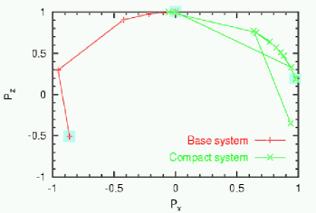
Figure 2.8: Rotation of the polarization vector in the $x$–$z$ plane in the nominal (‘short’) and an alternative (‘base’) CLIC final-focus system at 3 TeV centre-of-mass energy. The initial ($P_{x}$ = 0, $P_{z}$ = 1, i.e. purely longitudinal) and final polarization values are indicated by underlaid boxes.

During the beam–beam collision itself, because of beamstrahlung and the strong fields at 3 TeV, about 7% of effective polarization will be lost. About half of this loss is due to spin precession, the other half to spin-flip radiation. The latter is accompanied by a large energy change and thus does not affect the luminosity-weighted polarization at the nominal energy.

In view of the fairly large depolarization in collision, the polarization should be measured both for the incoming and for the spent beam. Therefore, we anticipate the installation of two Compton polarimeters on either side of the detector. A measurement resolution of 0.5% for the incoming beam would be comparable to that achieved at the SLC and expected for the other linear-collider designs. Reaching a similar resolution for the highly disrupted spent beam appears very challenging.

More details on polarization issues for CLIC at 3 TeV centre-of-mass energy can be found in Ref. [22].

2.6 $\gamma\gamma$ Collisions at CLIC

Gamma collider options have been considered in all linear collider studies. The energy region of 0.5–1 TeV is particularly well suited for $\gamma\gamma$ collisions from a technical point of view: the wavelength of the laser should be about 1 $\mu$m, i.e. in the region of the most powerful solid-state lasers and collision effects do not restrict the $\gamma\gamma$ luminosity [23, 24].

In the multi-TeV energy region the situation is more difficult: collision effects with coherent $e^{+}e^{-}$ pair creation in $\gamma\gamma$ collisions will be hard to avoid and may restrict the luminosity. The optimum laser wavelength increases proportionally with the energy. In addition, the required laser flash energy increases because of non-linear Compton scattering. Options for a 3-TeV photon collider based on 4–6 $\mu$m wavelength have been studied recently [25]. We summarize here the main results and give a tentative list of parameters and luminosity spectra.

Parameters of a possible photon collider at CLIC with $2E_{0}$ = 3000 GeV are listed in Table 2.3.

Table 2.3: Possible parameters of the photon collider at CLIC. Parameters of electron beams are the same as for $e^{+}e^{-}$ collisions.

$2E_{0}$	3000 GeV
$\lambda_{L}$  [$\mu$m]/$x$	4.4 / 6.5
$t_{L}$ $[\lambda_{{\rm scat}}]$	1
$N$ / 1010	0.4
$\sigma_{z}$  [mm]	0.03
$f_{rep}\times n_{b}$  [kHz]	15.4
$\gamma\epsilon_{x/y}$/10-6 [m$\cdot$rad]	0.68 / 0.02
$\beta_{x/y}$  [mm] at IP	8 / 0.15
$\sigma_{x/y}$  [nm]	43 / 1
$b$  [mm]	3
$L_{ee}$(geom)  [1034] cm-2s-1	4.5
$L_{\gamma\gamma}$ ($z>$ 0.8 $z_{m,\gamma\gamma}$)  [1034]	0.45
$L_{\gamma e}$ ($z>$ 0.8 $z_{m,\gamma e}$)  [1034]	0.9
$L_{ee}$ ($z>$ 0.65)  [1034]	0.6

The electron beam parameters shown in the table are the same as for $e^{+}e^{-}$ collisions. As discussed in Ref. [25], this is somewhat conservative, and there may be ways of decreasing electron beam sizes in collisions and potentially increase the $\gamma\gamma$ luminosity by a factor of about 3. The laser parameter $x$ = 6.5 approximately corresponds to the threshold for $e^{+}e^{-}$ creation for the non-linear parameter $\xi^{2}\approx$ 0.3. The corresponding wavelength is 4.4 $\mu$m. It is not clear at present which kind of laser would be best suited for a photon collider at this wavelength. Candidates are a gas CO laser, a free-electron laser, some solid-state laser or a parametric solid-state laser (the ‘short’ wavelength laser pulse is split in a non-linear laser medium into two beams with longer wavelength). The luminosity spectra obtained by a full simulation [26] based on the parameters quoted here are presented in Fig. 2.9.

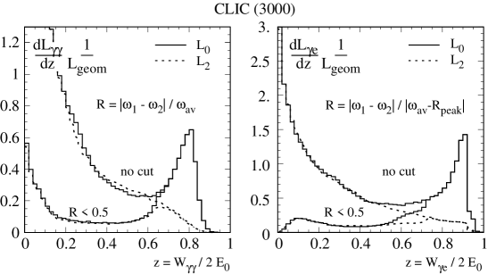
Figure 2.9: $\gamma\gamma$ (left) and $\gamma e$ (right) luminosity spectra at CLIC(3000). $L_{0},L_{2}$ are the luminosities with the total helicity of two colliding photons in the case of $\gamma\gamma$ collisions (or the total helicity of the colliding photon and electron in the case of $\gamma e$ collisions) equal to 0 and 2, respectively.

2.7 $e^{-}e^{-}$ Collisions at CLIC

While $e^{-}e^{-}$ collisions are considered an interesting option, not much effort was made to study it in detail. Most subsystems used to provide a positron beam can also be used for an electron beam, with minor modifications. The subsystems, which need larger changes, e.g. the injector that produces the beam, are usually simpler for electrons. The main concern is thus the beam–beam collision. In electron–positron collisions the two beams focus each other while they will deflect each other in electron–electron collisions. A preliminary study of the collision has been performed [27].

The simulations show that the total luminosity is reduced by a factor of roughly 4, but that the relative quality of the luminosity spectrum is better in the $e^{-}e^{-}$ collisions. For the part of the luminosity spectrum close to the nominal centre-of-mass energy, the reduction in $e^{-}e^{-}$ mode is thus only a factor of about 2.5 compared with $e^{+}e^{-}$. More remarkably, the background spectra of the $e^{-}e^{-}$ mode have a minuscule lower-energy tail, as is clearly shown in Fig. 2.10. Figure 2.11 shows the spent-beam and coherent pair production angular distributions, of major importance mainly for detector configuration studies. The number of beamstrahlung photons and coherent pairs is slightly reduced. The incoherent pair and hadronic background are reduced by a factor of 3 to 4. The angular distribution of the spent beam seems not to be worse than the one from $e^{+}e^{-}$ collisions. A detector designed for the latter should be perfectly capable of handling the $e^{-}e^{-}$ collisions as well.

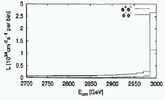
Figure 2.10: Absolute luminosity spectrum for the $e^{+}e^{-}$ and $e^{-}e^{-}$ cases. The bins have a width of 0.5% of the center-of-mass energy.

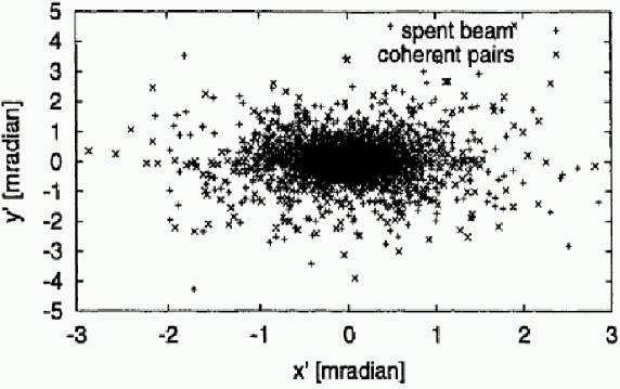
Figure 2.11: Angular distribution of the spent beam and the coherent pairs produced in the 3TeV collision

2.8 The CLIC Test Facility and Future R&D

The goals of the CLIC scheme are ambitious, and require further R&D to demonstrate that they are indeed technically feasible. The basic principle of two-beam acceleration with 30 GHz accelerating structures has already been demonstrated in CLIC Test Facilities 1 and 2 (CTF1 and CTF2). The technical status of CLIC was recently evaluated by the International Linear Collider Technical Review Committee (ILC-TRC), which was nominated by the International Committee on Future Accelerators (ICFA) in February 2001 to assess the current technical status of the four electron–positron linear-collider designs in the various regions of the world. The report [28] identified two groups of key issues for CLIC: (i) those that were related specifically to CLIC technology, and (ii) those which were common to all linear collider studies (such as the damping rings, the transport of low-emittance beams, the relative phase jitter of the beams, etc.). The CLIC study is for the moment focusing its activities on the following five CLIC-technology-related issues, which were given either an R1 (R&D needed for feasibility demonstration or an R2 (R&D needed to finalize design choices) rating by the ILC-TRC.

1. Test of damped accelerating structures at design gradient and pulse length (R1)

2. Validation of drive-beam generation scheme with a fully-loaded linac (R1)

3. Design and test of damped ON/OFF power extraction structure (R1)

4. Validation of beam stability and losses in the drive-beam decelerator, and design of
   machine protection system (R2)

5. Test of relevant two-beam linac subunit (R2).

Answers to these key R1 and R2 issues will be provided by the new CLIC Test Facility (CTF3), which is being built to demonstrate the technical feasibility of the key concepts of the novel CLIC RF power generation scheme, albeit on a smaller scale and re-using existing equipment, buildings and technical infrastructure that have become available following the closure of LEP. A schematic layout of CTF3 is given in Fig. 2.12. CTF3 is being constructed in collaboration with INFN, LAL, Northwestern University (Illinois), RAL, SLAC, and Uppsala University.

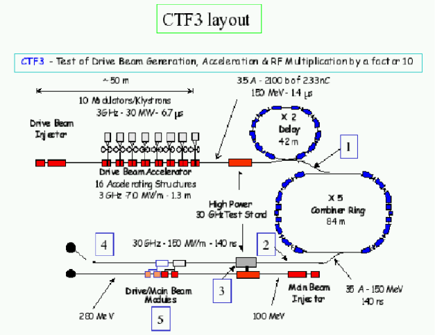
Figure 2.12: Schematic layout of CTF3

The principal aim is to demonstrate the efficient CLIC-type production of short-pulse RF power at 30 GHz from 3-GHz long-pulse RF power. This involves manipulations on intense electron beams in combiner rings using transverse RF deflectors as required in the CLIC scheme [29].

The following are some significant details of the scheme. A 140-ns-long train of high-intensity electron bunches with a bunch spacing of 2 cm is created from a 1.4-$\mu$s continuous train of bunches spaced by 20 cm. The 2-cm spacing is required for an efficient generation of 30-GHz RF power. This is done by interleaving trains of bunches and is done in two stages. The first combination takes place in the delay loop, where every other 140-ns slice of the 1.4-$\mu$s continuous train is sent round the 42-m (140-ns) circumference of the loop before being interleaved with the following 140-ns slice. This results in a reduction in the bunch spacing of a factor of 2 and an increase in the train intensity by a factor of 2. The second stage of combination — this time by a factor 5 — takes place in the combiner ring. After passing through the delay loop, the 1.4-$\mu$s train from the linac is made up of five 140-ns pulses with bunches spaced by 10 cm, and five interspaced 140-ns gaps. The combiner ring combines these five pulses into a single 140-ns pulse using a novel system of beam interleaving.

Progress CTF3 to date is as follows. Preliminary tests of bunch interleaving with five trains using a new gun and a modified version of the old LEP injector complex (LPI linac and EPA ring) at very low beam current were successfully completed in November 2002, and the results are summarized in Fig. 2.13. This result confirms the basic feasibility of the scheme. In December 2002 the old LPI linac was dismantled and in June 2003 the new CTF3 injector was installed. A bunched beam of the nominal current, pulse length and energy was obtained from the injector for the first time in August 2003.

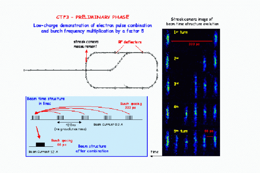
Figure 2.13: Low-charge demonstration of electron pulse combination and bunch frequency multiplication by a factor 5 in CTF3

Good progress has also been made with CLIC machine studies. The following steps have been achieved within the 30-GHz CLIC RF structure programme.

• Peak accelerating gradients of almost 200 MV/m have been obtained with short (16-ns) RF pulses with a 30-GHz molybdenum-iris accelerating structure — a comparative conditioning curve for three different materials is given in Fig. 2.3.

• A new fully-optimized design of the 30-GHz damped accelerating structure has been made, with significantly lower long-range transverse wakefields, which allow shorter bunch spacings and hence shorter pulse lengths.

• A new RF design of the 30-GHz power-generating structure has been proposed, with the ability to turn the power ON and OFF.

• The CLIC Stabilization Study Group has stabilized a prototype CLIC quadrupole to the level of 0.5 nm using commercially available equipment. Beam dynamics simulations of the main beams in the different parts of the machine have been integrated to give results with fully-consistent conditions.

2.9 Summary

We have summarized in this chapter the aims and status of the CLIC study, with emphasis on features related to its physics performance. The objective of a compact high-energy complex dictates the choice of a high accelerating gradient, requiring a high-frequency accelerating structure based on a two-beam approach. Accelerating structures capable of over 150 MV/m at 30 GHz have been operated successfully with short RF pulses in CTF2. Though optimized for a nominal centre-of-mass energy of 3 TeV with a design luminosity of 10³⁵ cm^-2s^-1, CLIC parameters for other energies between 0.5 and 5 TeV have also been proposed.

We have also discussed the principal machine characteristics that control the achievable luminosity, including the horizontal beam size, the bunch charge and the vertical beam size. The latter is constrained by the emittance produced in the damping ring, and its subsequent growth in the bunch compressor, the main linac and the beam delivery system. Further studies of the damping ring are needed, as are further studies of the effects of dynamical imperfections. In view of the small beam size, good alignment and stability of the CLIC components are crucial, and seem possible in a quiet site such as a tunnel through the molasse rock in the neighbourhood of CERN.

The scaling of CLIC parameters with the centre-of-mass energy has been discussed, and there are good prospects for polarized beams, $\gamma\gamma$ and $e^{-}e^{-}$ collisions. Principal R&D issues have been identified by the CLIC team and the Loew Panel. The CLIC Test Facility 3 (CTF3) now under construction at CERN will address the most critical R1 issues, and should enable the technical feasibility of CLIC to be established within a few years.

Chapter 3 EXPERIMENTATION AT CLIC

The definition of the CLIC programme in the multi-TeV range still requires essential data; these will become available only after the first years of LHC operation and, possibly, also the results from $e^{+}e^{-}$ collisions at lower energy. At present we have to envisage several possible scenarios for the fundamental questions to be addressed by accelerator particle experiments after the LHC.

It is therefore interesting to consider benchmark physics signatures for assessing the impact of the accelerator characteristics on experimentation and for defining the needs on the detector response. Each physics signature may signal the manifestation of different physics scenarios, possibly beyond those we envisage today. Nevertheless, the results of these studies should be generally applicable also to those other processes, having similar characteristics.

While considering experimentation at a multi-TeV collider, it is also interesting to verify to which extent extrapolations from experimental techniques successfully developed at LEP, and subsequently extended in the studies for a TeV-class linear collider, are still applicable. This has important consequences on the requirements for the experimental conditions at the CLIC interaction region and for the definition of the CLIC physics potential.

Four main classes of physics signatures have been identified. These are: resonance scans, electro-weak fits, multijet final states and missing energy and forward processes. Their sensitivities to the characteristics of the luminosity spectrum and the underlying accelerator-induced backgrounds differ significantly. Results of detailed simulations of several physics processes representative of each of these classes of physics signatures are discussed in the subsequent chapters. A physics matrix summarizing the various processes studied in detail for CLIC, with their interdependence on these classes of physics signatures and the aspects of the machine parameters, is given in Tables 3.1 and 3.2.

This chapter discusses the issues related to the experimental conditions at CLIC, the conceptual design for the detector and the software tools developed and used for simulation.

Table 3.1: Physics signatures and CLIC physics programme: matrix of the simulated processes

Physics	Higgs	SUSY	SSB	New gauge	Extra
signatures	sector			bosons	dimensions
Resonance scan		$\tilde{\mu}$	D-BESS	$Z^{\prime}$	KK
		thresholds			resonances
EW fits				$\sigma_{f\bar{f}},\,A^{f\bar{f}}_{\rm FB}$,	$\sigma_{f\bar{f}},\,A^{f\bar{f}}_{\rm FB}$,
Multijets	$H^{+}H^{-}$
	$H^{0}A^{0}$
	$H^{0}H^{0}\nu\bar{\nu}$
$E_{\rm miss}$, Fwd	$H^{0}e^{+}e^{-}$	$\tilde{\ell}$	$WW$
		$\chi^{0}_{2}$	scattering

Table 3.2: Physics signatures and CLIC accelerator parameters

Physics	Beam-	Beam	$e^{+}$	Pairs	$\gamma\gamma$ bkgd
signatures	strahlung	$E$ spread	polarization
Resonance scan	Stat. shape syst.	Shape syst.	Couplings	$\Gamma_{bb},_{cc},_{tt}$	$\Gamma_{bb},_{cc},_{tt}$
EW fits	Unfold boost		Polarization	$b\bar{b}$, $c\bar{c}$	$\cos\theta_{\rm min}$
			measurement	tags	bkgd flavour
Multijets	5-C fit			Tags for	Fake jets
				jet pairing
$E_{\rm miss}$, Fwd	$\theta_{\rm miss}$			Fwd tracking	$E_{\rm hem},\,E_{T}$

3.1 CLIC Luminosity

In order to obtain the required high luminosity the beams need to have very small transverse dimensions at the collision point of a linear collider. This leads to strong beam–beam effects and subsequently to a smearing of the luminosity spectrum and an increase of the background. The main beam parameters and background numbers are summarized in Table 3.3.

Table 3.3: The parameters of CLIC at $E_{c.m.}$ = 500 GeV and $E_{c.m.}$ = 3 TeV. For the latter energy two parameter sets are given: the first one is used to evaluate the background. The second set has been used for the ILC-TRC; it takes into account some recent findings of the structure research and beam-delivery system. The first set is used for background evaluation, as the second set is going to evolve soon, and because it yields higher background levels, so that it presents a more conservative view of the conditions. It should be noted that the beam sizes $\sigma_{x}$ and $\sigma_{y}$ are determined by fitting the results of full tracking with normal distributions. For background and luminosity the full tracking is used, including non-linear effects. $E_{c.m.}$: centre-of-mass energy, ${\cal L}$: actual luminosity, ${\cal L}_{0.99}$: luminosity with $E_{c.m.}>$ 0.99 $E_{c.m.,0}$, $f_{\rm rep}$: repetition frequency, $N_{\rm b}$: number of bunches per train, $\Delta_{\rm b}$: distance between bunches, $N$: number of particles per bunch, $\sigma$: bunch dimensions at IP, $\epsilon$: normalized emittances, $\delta$: average energy loss, $n_{\gamma}$: number of photons per beam particle, $N_{\perp}$: number of particles from incoherent pair production, produced with $p_{\perp}>$ 20 MeV and $\theta>$ 0.15, $N_{\rm hadr}$: number of hadronic events, $N_{\rm MJ}$: number of minijet pairs at $p_{\perp}>$ 3.2 GeV/$c$; for $E_{c.m.}$ = 3 TeV this has a significant theoretical uncertainty.

	$E_{c.m.}$ (TeV)		0.5	3	3
	${\cal L}$ (1034cm-2s-1)		2.1	10.0	8.0
	${\cal L}_{0.99}$ (1034cm-2s-1)		1.5	3.0	3.1
	$f_{\rm rep}$ (Hz)		200	100	100
	$N_{\rm b}$		154	154	154
	$\Delta_{\rm b}$ (ns)		0.67	0.67	0.67
	${N}$ (1010)		0.4	0.4	0.4
	${\sigma_{z}}$ ($\mu$m)		35	30	35
	${\epsilon_{x}}$ ($\mu$m)		2	0.68	0.68
	${\epsilon_{y}}$ ($\mu$m)		0.01	0.02	0.01
	${\sigma_{x}^{*}}$ (nm)		202	43	$\approx$ 60
	${\sigma_{y}^{*}}$ (nm)		$\approx$ 1.2	1	$\approx$ 0.7
	${\delta}$ (%)		4.4	31	21
	${n_{\gamma}}$		0.7	2.3	1.5
	$N_{\perp}$		7.2	60	43
	$N_{\rm hadr}$		0.07	4.05	2.3
	$N_{\rm MJ}$		0.003	3.40	1.5

3.1.1 Beam–Beam Interaction

During collision in an electron–positron collider, the electromagnetic fields of each beam accelerate the particles of the oncoming beam toward its centre. In CLIC this effect is so strong that the particle trajectories are significantly changed during the collision, leading to reduction of the transverse beam sizes, the so-called pinch effect. This enhances the luminosity but since it bends the particle trajectories it also leads to the emission of beamstrahlung, which is comparable to synchrotron radiation and reduces the particle energy. The average number of photons emitted is of the order of 1, so the impact on the centre-of-mass energy of colliding particles is somewhat comparable to initial-state radiation.

The produced beamstrahlung photons also contribute to the production of background. In the case of CLIC at high energies, the largest number of particles is expected from the so-called coherent pair creation. In this process a real photon is converted into an electron–positron pair in the presence of a strong electromagnetic field. The cross section for this process depends exponentially on the field strength and the photon energy. It is therefore very small at $E_{\rm c.m.}$ = 500 GeV but very important at $E_{\rm c.m.}$ = 3 TeV.

Programs have been developed to simulate the pinch effect as well as the production of beamstrahlung and the different sources of background. For our estimates we use GUINEAPIG [2].

For the old reference parameters, each particle emits on average 2.3 photons per bunch crossing, see Table 3.3. This corresponds to an average energy loss of about 30%. With the new parameters this is reduced to 1.5 photons per particle and a loss of about 20%. The number of coherent pairs is less than an order of magnitude smaller than the number of beam particles. They will thus give rise to some notable electron–electron and positron–positron luminosity.

3.1.2 Luminosity Spectrum

Not all the electron–positron collisions will take place at the nominal centre-of-mass energy. Several sources for an energy reduction of the initial-state particles exist. Each bunch has an initial energy spread of about $\sigma_{E}/E\approx$ 3 $\times$ 10^-3, the bunch-to-bunch as well as pulse-to-pulse energies vary and the beamstrahlung leads to energy loss during the collision. The bunch-to-bunch as well as pulse-to-pulse energy variations should be small, better than 0.1% peak to peak. While the feasibility of such a tight tolerance has been studied for the static bunch-to-bunch variation [3], further studies remain to be performed. The main sources of energy spread will, however, remain the single-bunch energy spread and the beamstrahlung. Most of the single-bunch energy spread is due to the single-bunch beam loading in the main linac, i.e. the fact that a particle in the head of a bunch extracts energy from the accelerating RF structure, so a particle in the tail sees a reduced gradient. In addition, because of the bunch length, not all particles are accelerated at the same RF phase, which changes the gradient they experience.

In principle the energy spread in the main linac could be reduced somewhat below the current reference value. This however would compromise the beam stability and would thus probably imply a reduction in bunch charge and consequently in luminosity.

In the collision, beam particles lose energy because of beamstrahlung. This limits the maximum luminosity that can be achieved close to the nominal centre-of-mass energy. The lower-energy collisions can also compromise the performance of experiments as they add to the background and make cross section scans more difficult. For otherwise fixed parameters, the beamstrahlung is a function of the horizontal beam size. A larger horizontal beam size leads to the emission of fewer beamstrahlung photons and consequently to a better luminosity spectrum. However, the total luminosity is reduced. Figure 3.1 shows the luminosity for the nominal CLIC parameters as a function of the horizontal beam size. On the right-hand side the total luminosity above $\sqrt{s}\geq$ 0.99 $E_{c.m.,0}$ is shown.

Figure 3.1: Left: Total luminosity and the luminosity with $E_{c.m.}\geq$ 0.99 $E_{c.m.,0}$ as a function of the horizontal beam size. Right: The fraction of the luminosity with $E_{c.m.}\geq$ 0.99 $E_{c.m.,0}$.

It should be noted that also the coherent pairs contribute to luminosity. While they increase the $e^{+}e^{-}$ luminosity by some percent (mainly at low centre-of-mass energies), they create $e^{-}e^{-}$ (and $e^{+}e^{+}$) collisions, where an electron, from a coherent pair produced in the positron beam, collides with the electron beam (and vice versa). Also there will occur a small number of $e^{-}e^{+}$ collisions, where the initial-state particles come from the wrong direction.

3.2 Accelerator-Induced Backgounds and Experimental Conditions

The characteristics of experimentation at CLIC will depend significantly on the levels of backgrounds induced by the machine and their impact on the accuracy in reconstructing the $e^{+}e^{-}$ collision properties. Compared with the benign conditions experienced at LEP/SLC, and also with those anticipated for a 500 GeV linear collider, at the CLIC multi-TeV energies, $e^{+}e^{-}$ events will lose part of their signature cleanliness, and resemble LHC collisions. This is exemplified by the local track density, due to physics events and backgrounds expected at CLIC, when compared with lower energy linear colliders and LHC experiments (see Table 3.4).

Table 3.4: Local track density on the innermost vertex tracker layer for different LC designs and $\sqrt{s}$, compared with those expected at the LHC

LC	$\sqrt{s}$ (TeV)	R (cm)	Hits mm-2 BX-1	25 ns-1	train-1
CLIC	3.0	3.0	0.005	0.18	0.8
NLC	0.5	1.2	0.100	1.80	9.5
TESLA	0.8	1.5	0.050	0.05	225.0
ATLAS	14	4.5	0.050	0.05
ALICE	5.5/n	4.0	0.900	0.90

The anticipated levels of backgrounds at CLIC also influence the detector design. There are two main sources of backgrounds: those arising from beam interactions, such as parallel muons from beam halo and neutrons from the spent beam, and those from beam–beam effects, such as pair production and $\gamma\gamma\to$ hadrons. Beam dynamics at the interaction region also set constraints on the detector design: the beam coupling to the detector solenoidal field limits the strength of the magnetic field.

3.2.1 Beam Delivery System

The beam delivery system (BDS) is the section of beam line following the main linac and extending through the interaction region to the beam dump. Its task is to transport and demagnify the beam, to bring it into collision with a counter-propagating beam, and finally to dispose of the spent beam. A collimation system, which provides a tolerable detector background and ensures machine protection against erroneous beam pulses, is also part of the BDS.

The CLIC BDS is a modular design, consisting of energy collimation, betatron collimation, final focus, interaction region, and the exit line for the spent beam. Table 3.5 lists the present design optics and beam parameters for the CLIC BDS at two different energies. Figure 3.2 shows the 3 TeV optics (from the end of the linac to the interaction point).

Table 3.5: Final-focus (FF), collimation system (CS), and beam parameters at 3 TeV and 500 GeV cm energy. Emittance numbers refer to the entrance of the BDS. The quoted spot sizes refer to the rms values obtained by particle tracking and are larger than the ‘effective’ beam sizes, which determine the luminosity.

Parameter (unit)	Symbol	3 TeV	500 GeV
FF length (km)		0.5	0.5
CS length (km)		2.0	2.0
BDS length (km)		2.5	2.5
Hor. emittance ($\mu$m)	$\gamma\epsilon_{x}$	0.68	2.0
Vert. emittance (nm)	$\gamma\epsilon_{y}$	10	10
Hor. beta function (mm)	$\beta_{x}^{\ast}$	6.0	10.0
Vert. beta function (mm)	$\beta_{y}^{\ast}$	0.07	0.05
Effective spot size (nm)	$\sigma_{x,y}^{\ast}$	65, 0.7	202, 1.2
Bunch length ($\mu$m)	$\sigma_{z}^{\ast}$	35	35
IP free length	$l^{\ast}$	4.3	4.3
Crossing angle (mrad)	$\theta_{c}$	20	20
Repetition rate (Hz)	$f_{\rm rep}$	100	200
Luminosity ($10^{34}$ cm-2s-1)	$L_{0}$	8	2

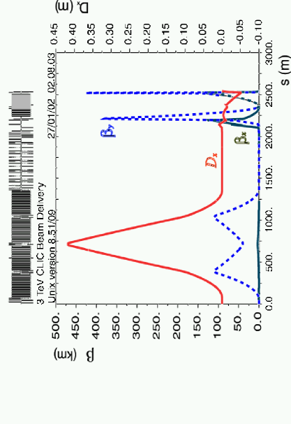
Figure 3.2: Optics of the 3-TeV CLIC beam delivery system. The collision point is on the right, at 2.6 km.

The system length is kept constant, independently of the energy. Only the sextupole strengths and bending angles are varied as the centre-of-mass energy is raised from 500 GeV to 3 TeV. This implies lateral displacements of magnets by up to 10–20 cm. The vertical IP beta function is squeezed down to values of 50–70 $\mu$m in order to optimize the luminosity. These beta functions are still comfortably large compared with the rms bunch length. In simulations, the target luminosity is reached at 3 TeV, and about twice the target value for 500 GeV. A solution for the design of the final quadrupole has been demonstrated, based on permanent-magnet material [4]. Typical synchrotron radiation fans inside the two final quadrupoles are depicted in Fig. 3.3, for an envelope covering 14$\sigma_{x}$ and 83$\sigma_{y}$. The requirement that synchrotron-radiation photons do no hit the quadrupoles on the incoming side determines the collimation depth.

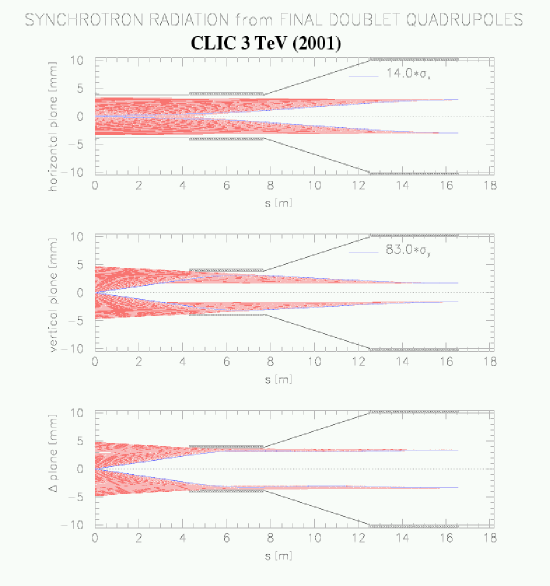
Figure 3.3: Synchrotron radiation fans at 3 TeV with beam envelopes of 14$\sigma_{x}$ and 83$\sigma_{y}$ (Courtesy O. Napoly [9]).

Collimation efficiency, energy deposition by lost particles and photons along the beam line, and muon background have been studied by various authors [5, 6, 7], and were found to be acceptable. Collimator wakefields and collimator survival have been taken into account in the design optimization [8].

A recent extended review of the present BDS designs for centre-of-mass energies of 3 TeV and 500 GeV can be found in Ref. [8]. The final focus has also been discussed in Refs. [9, 10], and the collimation system in Refs. [10, 11].

3.2.2 Muon Background

The rate of muons, produced as secondary particles in the collimation of high-energy (1.5 TeV) electrons’, can be substantial and requires a reliable simulation.

First estimates for CLIC have been obtained, based on the MUBKG code developed for TESLA [12] interfaced to GEANT3 for the simulation of the energy loss of the muons.

Figure 3.4 shows some simulated tracks of muons, produced at the first, horizontal spoiler (SPX1) and reaching the detector, which is located at about 3 km. The figure also shows the position of three optional, magnetized (2 T) iron ‘tunnel fillers’, each 10 or 30 m thick. They should be considered as a first attempt at implementing a dedicated muon protection system, as their properties and locations have not yet been optimized.

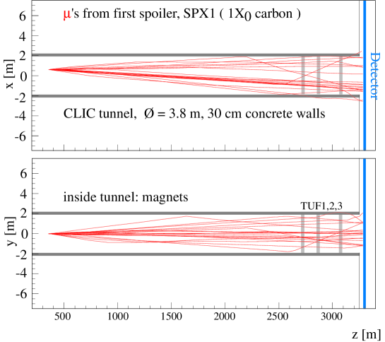
Figure 3.4: Tracking of muons, produced at the first spoiler, through the beam delivery system up to the detector region. Top is the horizontal and bottom the vertical plane.

Tracks that reached the detector region were input to a GEANT3-based detector simulation. Figure 3.5 shows the muon background overlayed on a physics event in the CLIC detector.

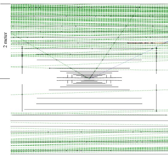
Figure 3.5: Physics event ($e^{+}e^{-}\to\tilde{\mu}\tilde{\mu}\to\chi^{0}_{1}\mu\chi^{0}_{1}\mu$) and muon background (in this case 1650 $\mu$ tracks) as seen in the detector simulation

The simulation allows the prediction of the ratio $r_{e\mu}$ of beam particles removed by the collimation system to the number of muons reaching the detector. For an estimate of the muon flux in the detector, assumptions have to be made about the fraction of halo electrons in the beam that will hit the collimators. The amount of beam particles in the tails is difficult to predict, but it is generally expected to be small. Here, the fraction hitting the first spoiler was assumed to be $f_{\rm tail}$ = 10^-3. With the parameters in Table 3.6, and for the two (e⁺ and e^-) beams in CLIC, we estimate that 2$N_{\rm e}\,N_{\rm b}\,f_{\rm tail}\,c_{\mu}/r_{e\mu}\approx$ 2.7 $\times$ 10⁴ muons per bunch train crossing would reach the detector. With a muon protection system of three tunnel fillers, their number could be reduced to 4000 muons per train, or 26 per bunch crossing.

Table 3.6: Parameters chosen to estimate the muon flux at the detector

Parameter	Symbol	Value
Beam energy	$E$	1.5 TeV
Number of $e^{+}$, $e^{-}$ per bunch	$N_{e}$	4 $\times$ 109
Bunches per train	$N_{\rm b}$	154
Fraction of tail particles	$f_{\rm tail}$	10-3
Secondaries and other processes	$c_{\mu}$	2
$e/\mu$ ratio without TUF	$r_{e\mu}$	9.2 $\times$ 104
$e/\mu$ ratio with TUF	$r_{e\mu}$	6.2 $\times$ 105

The factor of $c_{\mu}$ = 2 is based on more complete simulations for TESLA at 250 GeV; it accounts for muon production processes that were not included in the GEANT3 simulation used here, such as muon production from secondary photons in the cascade, $e^{+}e^{-}$ annihilation and hadronic muon production [12].

While the rate is modest and will not deteriorate the tracker when based on, say, silicon, the effect could be substantial for calorimetric measurements due to catastrophic radiation events. GEANT4 was used to estimate the amount of high energy showers that could be produced by the high energy muons. The expected muon background spectrum at the surface of the detector, shown in Fig. 3.6 (left), from Ref. [13], was used to shoot muons into a block of iron of 8 interaction lengths. This corresponds to a typical endcap of a calorimeter. Using approximately 10⁶ muons, the resulting spectrum of the energy released in the block is shown in Fig. 3.6 (right), for energy releases larger than 100 GeV. About 0.15% of the muons of this spectrum may leave a large energy shower in the calorimeter. Future studies will need to develop tools to recognize these showers, including the investigation of calorimeter techniques.

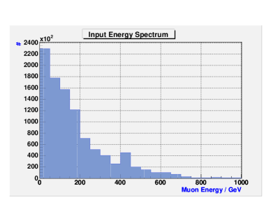
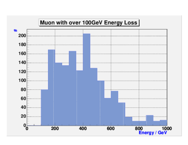
Figure 3.6: Left: The energy spectrum of the background muons that hit the detector surface; Right: The energy deposited in a block of iron of 8 interaction lengths

More recently, a fully integrated approach using GEANT4 has been implemented. This includes the conversion of photons into a pair of muons in the presence of the fields of the nucleus and the annihilation of high energy positrons with atomic electrons [14, 15]. The GEANT4 program has also been extended to perform the tracking through the machine lattice and materials in a combined, flexible manner. The simulation can then be built from an existing machine description, allowing for background optimization during the machine design phase [6].

3.2.3 Neutron Background

No detailed study of the neutron flux expected from the spent beam has been performed. Some estimate of the flux induced by the hadrons produced in the beam–beam interaction is given in the next section. Regarding the spent beam, a simple estimate of the neutron flux can be based on the giant resonance production of neutrons. The low energy neutrons from this process tend to fly in all spatial directions with an almost equal probability. The high energy neutrons from other processes tend to move more in the direction of the incoming particle beam and will thus fly away from the detector.

The total number of neutrons produced depends on the material of the beam dump. With water, about one neutron is produced per 32 GeV of incoming photon or electron energy. Neglecting backscattering and shielding, the flux at the interaction point would then be 4.6 $\times$ 10¹³ cm^-2 per year (10⁷ s) of operation, for a dump to IP distance of 100 m. While a good fraction of the neutrons can be shielded, this shielding needs to have a hole to let the spent beam pass. While the electron and positron beams can in principle be bent in such a way that there remains no direct line of sight between beam dump and detector, this is not possible for the photon beam. The best (and probably only) place where the vertex detector can be shielded from the photon dump is inside the detector. Such a mask can reduce the flux by about three orders of magnitude [16]. In the present case this would yield a flux of about 4.6 $\times$ 10¹⁰ cm^-2 per year. Increasing the distance between dump and interaction point would reduce this value further. However, a careful, detailed study of this problem, including backscattering of neutrons, remains to be done.

3.3 Beam–Beam Backgrounds and their Impact

During the collision a number of particles are produced as background. Beamstrahlung photons and coherent pairs have already been mentioned. Their number is comparable to the number of beam particles, so they strongly constrain the detector design. Further electron–positron pairs are created by incoherent two-photon production. Hadrons are produced in a similar fashion. The number of these particles is small enough not to modify the beam–beam interaction any further, but they still have a significant impact on the detector design.

3.3.1 Coherent Pairs

The number of coherent pairs is quite large: at $\sqrt{s}$ = 3 TeV about 7 $\times$ 10⁸ pairs are produced per bunch crossing. The spectrum of the particles is shown in Fig. 3.7; it peaks at about 100 GeV and has a long tail toward high energies, almost reaching the full beam energy. At low energies ($\approx$ 10 GeV) the production is strongly suppressed.

Figure 3.7: The energy spectrum of the coherent pairs produced during the collision

The particles initially have small angles with respect to the beam axis. While a newly created electron that flies in the direction of the electron beam is focused by the positron beam, a positron going in the same direction is deflected away from the axis. Since the energy of a typical coherent pair particle is lower than that of a beam particle, the angle after the collision is significantly larger. The coherent pair production thus significantly affects the aperture requirement for the spent beamline. Since the number of coherent pairs is very large, one has to avoid losing even a small fraction of them in the detector region. In order to achieve a reasonable statistics, a large number of particles thus has to be simulated, requiring a significant amount of computing time.

3.3.2 Spent Beam

The spent beam consists mainly of the beam particles, the secondary beamstrahlung photons and the coherent pairs. While the former two components are confined to relatively small angles (of the order of 1 mrad), the latter can reach larger angles. In order to avoid more losses in the detector region, an exit aperture must be provided for these particles. Simulations with GUINEAPIG showed that an aperture of about 10 mrad around the axis of the spent beam is sufficient [17]. Since space is needed around the axis of the incoming beam for the final-focus quadrupole, a total crossing angle of about 20 mrad appears reasonable.

3.3.3 Incoherent Pairs

The production of $e^{+}e^{-}$ pairs through two-photon processes can lead to significant background at all energies. The main contributions arise from $ee\to eee^{+}e^{-}$, $e\gamma\to ee^{+}e^{-}$, and $\gamma\gamma\to e^{+}e^{-}$, where the photons are from beamstrahlung. In the beam–beam simulations, the processes that include one or two beam particles are calculated by replacing the particle with the equivalent photon spectra. This allows the effect of the beam size and the strong beam fields onto the cross sections to be taken into account.

It is important to track the produced particles through the fields of the beams, since they can be strongly deflected. Figure 3.8 shows particles after the collision. For the bulk of these, a clear correlation is visible between the maximum particle angle and the transverse momentum. These particles were produced at small angles and obtained most of their transverse momentum from the deflection by the beams. A few particles above this edge were produced with large angles and transverse momenta. They can produce significant background in the vertex detector.

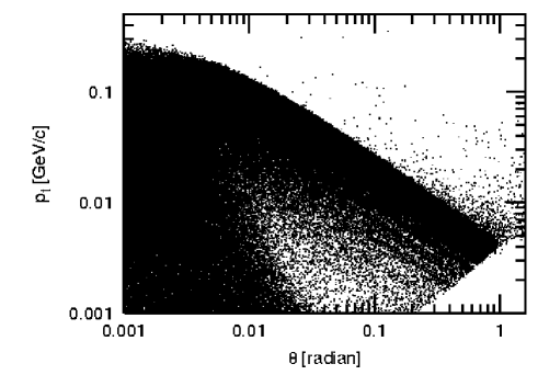
Figure 3.8: Angle and transverse momentum of the incoherent pairs after the collision. Only particles with an energy larger than 5 MeV were tracked

3.3.4 Hadronic Background and Resulting Neutrons

Two-photon collisions can also lead to the production of hadrons. The cross section for this process is not very well established at higher centre-of-mass energies, and measuring it will be an interesting experiment at a future linear collider. In order to estimate the number of these events, a simple parametrization of the cross section [18] is done with GUINEAPIG. For the old reference parameters, this simulation yields about 4 events with a centre-of-mass energy above 5 GeV per bunch crossing (Fig. 3.9). For the new beam parameters this number is reduced to 2.3 events per bunch crossing.

Figure 3.9: Left: The average number of hadronic events per bunch crossing as a function of the visible energy above a given cut angle $\theta$. Right: The number of events as a function of the transverse energy.

The final states of the hadronic background were simulated using PYTHIA. The average visible energy in the detector is about 90 GeV per bunch crossing. The hadronic background also causes charged hits in the vertex detector. The highest density of these hits is 0.25 hits mm^-2. While this is still lower than the $\simeq$ 1 hit mm^-2 due to incoherent pairs, it is still a sizeable contribution. A database containing the hadronic background of about 2000 bunch crossings has been made available [19] and can be accessed using the HADES library (see Section 3.5.4) [20].

The secondary neutron flux from these hadronic events has also been simulated, yielding a maximum flux of 3 $\times$ 10⁹ $n$ cm^-2 per year (= 10⁷ s) of operation [21]. The flux is highest around the masks and smaller around the IP.

3.3.5 Crossing Angle

In CLIC the beams will collide with a full crossing of 20 mrad. Lower limits of this crossing angle arise from the so-called multibunch kink instability and the necessity to extract the spent beam from the detector with minimal losses. An upper limit is imposed by the detector solenoidal field, which, in the presence of a crossing angle, affects the beams, leading to the emission of synchrotron radiation and the subsequent increase of the beam spot size.

To avoid the luminosity reduction normally associated with collisions at a crossing angle, the so-called crab-crossing cavities should be used. These cavities add a small horizontal kick to the beam particles, depending on their longitudinal position in the bunch. This scheme allows the bunches to collide head-on.

3.3.5.1 Lower limit of the crossing angle

During the beam collision a large number of electron–positron pairs is created. These particles carry about $1\%$ of the total beam energy and are deflected by the strong electromagnetic fields of the beams. Consequently they can lead to large losses in the line for the spent beam. While the detector is shielded against the resulting secondaries by a tungsten mask, some of these are still of concern, in particular neutrons. In addition, the sheer energy deposition may lead to problems. In particular, the tolerance for the position stability of the final quadrupoles, which are inside the detector and must not move by more than $\approx$ 0.2 nm, may be hard to meet. However, providing an exit hole lets all the particles through with an angle of less than 10 mrad and solves the problem [17]. This can be achieved with a crossing angle of at least 10 mrad. Since additional space is required for the quadrupole around the incoming beam a reasonable lower limit is $\theta_{c}\geq$ 20 mrad.

Another issue is the kick that the outgoing beam applies on the incoming one during the parasitic crossing inside the detector. This effect can be reduced by shielding the incoming beam line from the outgoing one, but to achieve this some material must be placed close to the IP. Another possibility is to increase the crossing angle in order to reduce the parasitic kicks. A sufficient suppression can be achieved with a crossing angle of $\theta_{c}$ = 20 mrad.

3.3.5.2 Beam coupling to the detector field

If the beams have an angle with respect to the detector solenoidal field, they will travel on a helix toward the collision point. By choosing an appropriate optics for the incoming beam, the associated effects can be compensated. However, in the solenoidal field the particles will emit synchrotron radiation, which modifies their energy and thus their trajectory slightly. As a consequence the beam-spot size will increase in the vertical direction. This effect can be reduced by decreasing either the detector solenoidal field or the crossing angle. A preliminary study indicates that for $B_{z}$ = 4 T a crossing angle of $\theta_{c}$ = 20 mrad is still acceptable [22]. However, the results depend significantly on the detector end fields, for which only a simple model was used in the study. Therefore it will be necessary to perform more precise simulations when a design for the detector solenoid becomes available.

3.3.6 Impact on the Vertex Detector Design

A crucial constraint on the detector design arises from the hits of incoherent pairs in the innermost vertex detector layer. An acceptable density of hits from background on the innermost layer is of $O(1)$ hits mm^-2 per readout cycle. Beyond this level the pattern recognition will be affected by the association of spurious hits to particle tracks and by the creation of ghost tracks. To allow some safety margin a target of not more than 1 hit  mm^-2 has been adopted. The number of hits in the vertex detector has been obtained using a full GEANT simulation. Figure 3.10 shows the expected hit density per beam pulse at different values of the radius $r$ of the innermost vertex detector layer as a function of the longitudinal position $z$. At $r$ = 30 mm the hit density reaches the limit of about 1 mm^-2, and this radius has therefore been adopted in the detector design. A higher detector solenoidal field could be used to further reduce $r$.

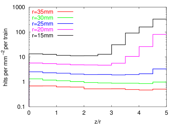
Figure 3.10: Number of hits per train as function of the ratio of the longitudinal position along the beam axis to the detector radius, for different values of the radius

Figure 3.11: Sketch of the mask layout

3.3.7 Mask Design

Another potentially important source of hits in the vertex detector is that of low-energy electrons and positrons from coherent pair creation; these are backscattered in the final quadrupoles and are then guided by the main solenoidal field back into the vertex detector [16]. The total number of hits from this source can be an order of magnitude larger than the direct hits. This effect can be suppressed by using a mask that covers the side of the quadrupole facing the detector. If the mask is covered with a low-$Z$ material, backscattering can be almost completely suppressed; graphite is currently considered. Figure 3.11 shows the full masking system, of which the part discussed here consists of the graphite and instrumented tungsten layers.

Originally the mask has been developed for a machine without a crossing angle [16] and it was found that it worked excellently as soon as the inner opening, through which the beam passes, is smaller than the vertex detector. In the presence of a crossing angle the situation is more complicated, as part of the vertex detector cannot be protected by the mask. One therefore has to provide further masking downstream, to prevent backscattering through the hole of the mask.

The inner mask also serves as a shield against neutrons, which are produced by the spent beam and backscattered into the detector. It has been shown that such a shield can reduce the neutron flux in the vertex detector by three orders of magnitude [16]. For this purpose, the opening in the mask needs to be smaller than the vertex detector; the crossing angle does not matter as the neutrons will mainly come antiparallel to the spent beam. The further the mask is from the IP the larger the opening must be to allow the passage of the spent beam. At the chosen distance of 2 m between mask and IP, the opening has a radius of 2 cm and satisfies both conditions.

Not all the coherently and incoherently produced pairs will pass the exit hole for the spent beam. The fraction that is lost in the detector produces secondary photons, which can cause severe background. A conical mask is employed to shield the detector. Currently a simplified geometry is used for this mask. The design is completely determined by the inner and outer opening angle, $\theta_{0}$ and $\theta_{1}$, and the distance to the IP at which the mask starts is chosen to be 1 m. The need to let the bulk of the pairs enter the mask then fixes the inner opening angle in the detector magnetic field of $B_{z}$ = 4 T. Figure 3.12 shows the distances from the detector axis reached by the incoherent pairs; they are similar for the coherent ones. To allow some margin an inner opening angle $\theta$ = 80 mrad is chosen. With an outer angle $\theta_{1}$ = 120 mrad one can expect the mask to suppress the photons sufficiently [16]. Optimization of the mask remains to be done, and in particular the instrumentation of this area needs to be considered.

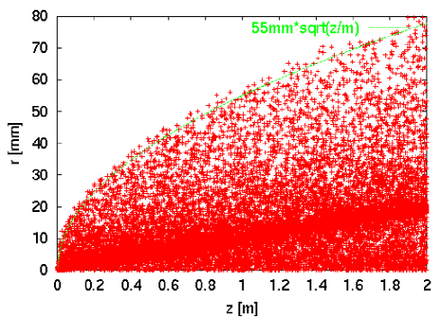
Figure 3.12: The particles from incoherent pair production in the spent beam

3.4 The Detector: Concept and Techniques

The concept of a detector for CLIC is greatly influenced by the experience gained at LEP/SLC and by the technical solutions being adopted for the LHC. The extrapolation of these principles to a detector for energies up to about 1 TeV, a factor of 5 more than at LEP, is already well advanced within the LC studies world-wide. As CLIC pushes the energy range up by another factor of 5, a major question arises on the validity of such an extrapolation for multi-TeV $e^{+}e^{-}$ physics.

In order to appreciate the different characteristics of events from multi-TeV $e^{+}e^{-}$ collisions, it is useful to consider that the jet multiplicity will reach fourteen, with large charged and neutral particle multiplicity. The $b$-hadrons will travel up to 20 cm, owing to the large boost in two-fermion events. The intense beam radiation will produce events boosted along the beam axis, and backgrounds will become of primary importance with significant minijet and pair production. There will be of the order of 2000 photons per bunch crossing, and 25000 muons per train, traversing the detector.

Table 3.7: Average reconstructed jet multiplicity in hadronic events at different $\sqrt{s}$ energies

$\sqrt{s}$ (TeV)	0.09	0.20	0.5	0.8	3.0	5.0
$\langle N_{\rm Jets}\rangle$	2.8	4.2	4.8	5.3	6.4	6.7

Studies of the detector concept for a 500 GeV LC have considered both a small and a large detector. The first consists of a compact Si tracker with high magnetic field ($B$ = 5–6 T). The large detector relies on a continuous time projection chamber (TPC) main tracker, has a lower magnetic field ($B$ = 3–4 T) and moves the calorimeter further away from the interaction region, which is advantageous for energy flow reconstruction based on a fine granularity.

At CLIC, the beam delivery system will constrain the solenoidal magnetic field of the detector to below about 6 T. We consider here a model for a large detector, which inherits much of the solutions adopted in the ECFA/DESY study for a 500–800 GeV LC, adapted to the experimental conditions expected at CLIC.

3.4.1 Vertex Tracker

A CLIC vertex tracker design may consist of a multilayered detector with very high 3-D space resolution and stand-alone tracking capabilities. At CLIC, the anticipated background from $e^{+}e^{-}$ pairs produced in the interaction of the colliding beams will limit the approach to the interaction region to about 3.0 cm, compared with $\simeq$ 1.5 cm foreseen for the lower energy projects. This is partly compensated by the increase of the short-lived hadron decay length due to the larger boost. At $\sqrt{s}$ = 3 TeV, the average decay distance of a $B$ hadron is 9.0 cm, in the two-jet process $e^{+}e^{-}\to b\bar{b}$, and 2.5 cm in multiparton $e^{+}e^{-}\to H^{+}H^{-}\to t\bar{b}\bar{t}b\to W^{+}b\bar{b}W^{-}\bar{b}b$ decays. Because of the large boost and large hadronic multiplicity, the local detector occupancy in $e^{+}e^{-}\to b\bar{b}$ events is expected to increase, by a factor of almost 10, to $>$ 1 particle mm^-1 from $\sqrt{s}$ = 0.5 TeV to $\sqrt{s}$ = 3.0 TeV. This indicates the need to design a large vertex tracker based on small-area pixel sensors, able to accurately reconstruct the trajectories of secondary particles originating few tens of centimetres away from the beam IP and contained in highly collimated hadronic jets. There are other background issues relevant to the conceptual design of a vertex tracker for CLIC. These are the rate of $\gamma\gamma\to$ hadrons events, estimated at 4.0 BX^-1, and the neutron flux, possibly of the order of 10¹⁰ 1-MeV-equivalent n cm^-2 year^-1. The need to reduce the number of $\gamma\gamma$ events overlapped to an $e^{+}e^{-}$ interaction requires fast time stamping capabilities, while the neutron-induced bulk damage has to be considered in terms of sensor efficiency reduction. Significant R&D is under way for meeting the requirements of a TeV-class $e^{+}e^{-}$ linear collider; further developments are expected when the issues related to the SLHC will be addressed.

Emerging silicon sensor technologies and possible paths for the upcoming R&D are discussed in the next section.

A detector consisting of seven concentric Si layers located from 3.0 cm to 30 cm from the beam IP and based on pixel sensors, with 20 ns time stamping and radiation hardness capabilities, demonstrated for their LHC applications can be considered as a baseline design for the vertex tracker. The layer spacing has been chosen to optimally sample the heavy hadron decay length, resulting in a closer spacing for the innermost layers (see Fig. 3.13).

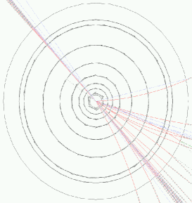
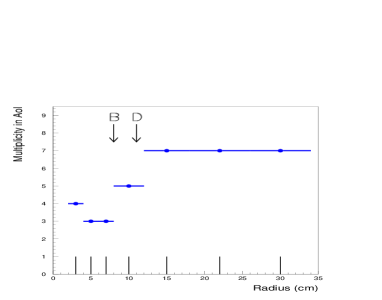
Figure 3.13: Display of a $e^{+}e^{-}\to b\bar{b}$ event at $\sqrt{s}$ = 3 TeV (left) with the detected hit multiplicity steps from the cascade decay of a long-flying $B$ hadron (right)

3.4.2 Trends in Si Sensor Developments and Future R&D

Silicon sensors have been very successfully employed in collider experiments for many years. They are based on well established technologies and their prices have dropped quite significantly over the years, making large-area trackers both feasible and affordable. Obvious advantages of Si pixel detectors are their accurate point resolution, of the order of 10 $\mu$m, true 3D reconstruction of the point of passage of the particle, and fast charge collection. The main drawback is certainly related to the relatively high material burden represented by the present sensors and related read-out electronics. R&D studies performed for the SLHC experiments to improve the radiation hardness of silicon devices have shown that fluences of several 10¹⁴ 1-MeV equivalent neutrons cm^-2 can be coped with, which is orders of magnitude higher than those expected at CLIC.

Tracking systems for future collider experiments will need very large area detectors with a macro-pad geometry (0.5 mm to 1 mm pixels). A large pixel granularity, with $<$ 50 $\times$ 50 $\mu$m² pixels, are required for vertex detectors. The time structure of the colliding beams at CLIC and SLHC, high-multiplicity events, and the precise tracking requirements will need time-stamping capabilities of $O$(1–10 ns). These challenging requirements call both for innovative detector technologies and readout electronics that profit from future nanoscale microelectronics technologies.

Based on the experience from the LEP silicon trackers and the past R&D work and production of prototype tracker systems, strip and pixel, for the LHC experiments, some preliminary guidelines can be drawn to direct the needed R&D on Si detectors for future tracking systems. Identified issues in designing and constructing large-area Si tracking systems (with detector areas of tens to hundreds of square metres) can be categorized as follows:

• Cost: present Si detector technology, based on crystal Si wafers, has reached an industrial maturity and the current production cost of about 10 CHF/cm² cannot realistically be expected to decrease significantly.

• Spatial resolution: LHC hybrid pixel detectors currently have a minimum pixel dimension of 50 $\mu$m, corresponding to the minimum pitch realistically feasible for the current bump bonding technology. The wafer thickness of 300 $\mu$m can be thinned down to 200 $\mu$m.

• Charge collection speed: the nominal charge collection time of a standard silicon detector is in the range of 10 ns to 20 ns.

• Radiation hardness: the R&D work on radiation hardness of crystal Si detectors done for the LHC experiments has shown that standard $n$-doped high-resistivity substrates reach the doping inversion at about 2 $~{}\times~{}$10¹³ $n$/cm² and sustain a displacement damage at a fluence of few 10¹⁴ $n$/cm². Above this limit, standard crystal Si detectors cannot be used.

• Interconnections: bonding between silicon detectors and readout ASICs, wire bonding for strips and bump bonding for pixel detectors, represents a substantial effort and expansive step in the construction of silicon strip and silicon pixel detector modules.

• Cooling: Si strip and pixel detectors in central LHC trackers operate at $-15^{\circ}$ C to control the leakage current and reverse annealing after radiation damage. This poses strong constraints on the design of cooling systems, substantially increasing the material budget.

Considering all these issues, it turns out that scaling up dimensions, improving spatial precision, radiation hardness, charge collection speed of future silicon trackers is a very challenging task, without a technological breakthrough based on emerging solid-state detector technologies, the cost issue not being the least obstacle. Thinner standard crystal Si (of order 100 $\mu$m) could in principle improve the detector

Table 3.8: Comparison of the different pixel sensor technologies

Properties	Standard planar crystal	3-D silicon	Monolithic CMOS pixel	a-Si:H pixel detector
	silicon		detector
Collection speed	10 ns	Short drift	Thermal drift	Short drift, high field
Electron transient t	20 ns	$<$1 ns	100 ns	2 ns
Holes transient t		1 ns	200 ns	150 ns
Thickness	300 $\mu$m	100–200 $\mu$m	2–8 $\mu$m	30–50 $\mu$m
MIP charge signal	24 000 $e^{-}$	10 000–20 000 $e^{-}$	100–500 $e^{-}$	1000–2000 $e^{-}$
Radiation hardness	3 $\times$ 1014	At least 1015 at + 20∘C	$<$ 1013,	$>$ 5 $\times$ 1015, limit not known,
			strong surface effects	self-annealing by mobile H
Fluence (n/cm2)	at – 20∘C
Operating temperature	– 20∘C, cryogenic	Room	Room	Room to 60∘C
Manufacturing cost	High	High	Low	Low
Field of applications	Microvertex detector	Small detector area,	Microvertex detector,	Large–area detector,
	tracker	fast timing, high	low radiation level,	macropad and microvertex,
		radiation level	slow readout	high radiation environment

speed and minimize voxel thickness for a better geometry. However, large-area thin-crystal detectors are impractical for outer-tracker systems and delicate for microvertex systems; furthermore, they do not solve the other issues mentioned above.

There are three novel solid-state detector technologies that are likely to have a significant impact on their design at future collider experiments. A comparison of the different pixel sensor technologies is given in Table 3.8.

3.4.2.1 3D sensors

3D detectors are a new generation of silicon sensors, which combine fast readout signals, low depletion voltage and full sensitivity, independently of the substrate thickness. This detector design was originally proposed by S. Parker and C. Kenney [23, 24], and is schematically represented in Fig. 3.14 (left). The process involved in the fabrication of 3D devices is a combination of traditional VLSI (Very Large System Integration) and Deep Reactive Ion Etching (DRIE), which was developed for micromechanical systems. DRIE allows microholes to be etched in silicon with a thickness-to-diameter ratio as large as 20 : 1. In the 3D detectors currently processed at Stanford, USA, by a collaboration involving scientists from Brunel (UK), Hawaii, The Molecular Biology Consortium (MBC), CERN, Stanford, ESRF and others, this technique is used to etch holes as deep as several hundred microns, at distances as short as 50 microns from one another. These holes are filled with polycrystalline silicon doped with either Boron or Phosphorus, which is then diffused into the surrounding single-crystal silicon to make the detector electrodes. The silicon substrate used for this process can be either p-type or n-type, and the crystal orientation is $<$ 100 $>$, where 1,0,0 represent the crystal plane coordinates. Silicon atoms line up in certain directions in the crystal. $<$ 100 $>$ corresponds to having a particular crystal plane at the surface, and is preferred for a better surface quality. Once the electrodes are filled, the polycrystalline silicon is removed from the surfaces, and the dopant is diffused. The same process is then used to fabricate ‘active edges’, or all around trench electrodes doped with either phosphorus or boron to properly complete the electric field lines. The presence of active edges reduces the dead volume around the detector to $<$ 10 $\mu$m, as can be seen from the $X$-ray beam scan in Fig. 3.14 (right). From this figure, obtained using the 2 $\mu$m, 12-keV beam line at the Advanced Light Source, Berkeley, it is possible to see the rapid turn on response of the detector at the edge and the partial response of the centre of the electrodes.

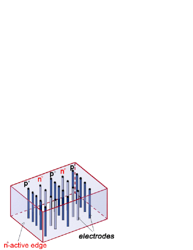
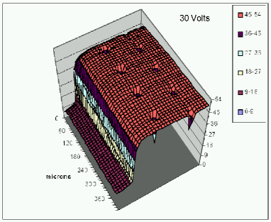
Figure 3.14: Left: Sketch of a 3D detector where the p+ and n+ electrodes are processed inside the silicon bulk. The edges are trench electrodes (active edges) and surround the sides of the 3D device making the active volume sensitive to a few microns from the physical edge. Right: Scan of part of a 3D detector performed with a 12 keV $X$–ray beam. The edge signal turn-on is visible on the left. The vertical scale represents the current pulse height in arbitrary units (also colour coded), and the distance between electrodes is 100 microns.

Similar tests have been performed with particle beams [25]. The new etching machines and the new etching techniques that are becoming available should allow one to reduce the electrode central part as much as possible. When the etching process is completed, aluminium can be deposited in a pattern that will depend on how the individual electrodes are to be read out.

A 3D detector, where all the electrodes have been connected together by an aluminium microstrip, is shown in Fig. 3.15 (left). The oscilloscope trace of its response to a minimum ionising particle is shown in Fig. 3.15 (right) [26]. The fast radiation-hard electronics used for this test, designed by the CERN microelectronics group dominates the rise time of the pulse, which was measured to be 3.5 ns and did not degrade after 1 $\times$ 10¹⁵ protons/cm². The same device was tested at 130 K. At this temperature the pulse rise timed improved to 1.5 ns while the full pulse width was measured to be less than 5 ns. The inter electrode spacing of these detectors was 100 mm. Devices with shorter spacing have been processed and should have an intrinsic charge collection time of $<$ 1 ns [23]. Tests with such devices and 0.13 microns electronics readout are in preparation.

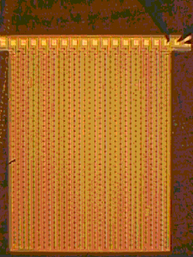
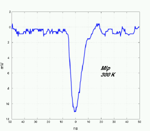
Figure 3.15: Left: 3D detector with microstrip readout configuration. The electrodes and the aluminium strips, which tie the rows of ${\rm p^{+}}$ and ${\rm n^{+}}$ electrodes, are clearly visible. The ${\rm p^{+}}$ strips end at the bonding pads (top). Right: Oscilloscope traces of mips of 3D detectors at room temperature. The rise time is 3.5 ns and is dominated by the readout electronics. The electrode spacing is 100 microns.

3.4.2.2 Monolithic Si sensors: MAPS

The integration of detector and electronics is particularly crucial in high-resolution silicon pixel detectors for microvertex applications, where a very high density of pixel elements has to be achieved. The monolithic approach [27, 28] is based on Active Pixel Sensor (APS) technology and utilizes the epitaxial layer of the CMOS wafer as detector substrate. The Monolithic Active Pixel Sensors (MAPS) detectors potentially provide unambiguous two-dimensional tracking, where the detecting element is inseparable from the readout electronics. In this approach, both the detector and the front-end readout electronics are integrated on the same silicon wafer, using standard CMOS fabrication processes. The development of MAPS detectors started with their use as photon detectors, in the visible band, where they are becoming increasingly popular at the expence of Charge Coupled Devices (CCDs). MAPS devices are detectors with a small-area readout section, yielding good noise performance. However, the charge collected originates from a thin active volume. In this approach, a thin, moderately doped, undepleted Si layer is used as radiation-sensitive volume, while the readout electronics is implemented on top of it. This particular structure makes the entire sensor surface sensitive (100% fill factor), as required for particle tracking. The sensitive volume is usually an epitaxial layer, which is available in modern CMOS processes, where it is grown on a highly, usually ${\rm p^{++}}$-type, doped substrate. The pixel readout electronics is placed in the ${\rm p}$-well. Because of the difference in doping levels (about 10³), the epitaxial layer junctions with the ${\rm p}$-well and the substrate acts as reflective barriers, confining the charge carriers.

The electron-hole collection is performed by thermal diffusion between ${\rm n}$-well electrodes. The charge-collection is then spread over several ${\rm n}$-well collecting electrodes. But MAPS devices have a low tolerance to radiation effects. Ionizing radiation induces surface effects that deteriorate charge collection, and displacement damage decreases the minority carrier lifetime, thus rapidly deteriorating the charge collection efficiency. Only NMOS transistors can be used in pixel circuits, which represents an important limitation for the circuit design of the pixel cell.

3.4.2.3 Hydrogenated amorphous Si on ASIC Technology

A seed R&D on the technology of deposition of hydrogenated amorphous silicon n.i.p layer on ASIC [29, 30] has shown that this detector technology has a great potential to solve present limitations of standard Si crystal detector technology.

One of the main advantages of such techniques is the potential cost reduction and the sensor integration with the readout electronics, as in pixel monolithic detectors. Compared with standard Si hybrid pixels, the deposition of a-Si:H on ASIC greatly simplifies the pixel detector fabrication (see Fig. 3.16). The problem of interconnections to the electronics is also solved. Another advantage is that a-Si:H semiconductor is extremely radiation-hard, thanks to a self-annealing process operated by mobile hydrogen (15%) within the amorphous tissue, and defects are continuously passivated. The intrinsic limit of radiation hardness is expected to be above 10¹⁵ ptcs cm^-2. An a-Si:H detector can also operate in a wide temperature range, from room temperature to up to $\simeq$ 60^∘ C, without affecting the charge collection efficiency. This feature represents a great simplification for the cooling systems, which are at present a bottleneck in the system design of the LHC trackers.

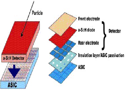
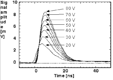
Figure 3.16: Amorphous silicon detector. Left: a schematic of a hydrogenated amorphous Si detector on ASIC. Right: The time behaviour of the signal for different polarization voltages showing the intrinsically fast charge-collection properties.

Preliminary results have demonstrated that charge collection is quite fast: 3 ns to 5 ns for electron carriers (see Fig. 3.16). High-energy electrons of  ⁶³Ni and ⁹⁰Sr have been measured with a short peaking time of 15 ns. However, a substantial R&D effort is essential to master the deposition technology of a-Si:H on ASIC. Several technological issues have to be mastered, in order to obtain an excellent a-Si:H, in particular a low dangling bond defect density, with a high deposition rate of 1 to 2 nm s^-1. The need for a low defect density is essential to deplete a thick intrinsic layer, 50 $\mu$m with reasonable bias voltages.

3.4.2.4 Readout electronics, microelectronics and design effort

The development of microelectronics will continue its pace towards nanoscaled transistor feature size. The particle physics community should monitor and understand how to profit from these technological advances, which have been a crucial basis for developing novel solid-state detector and radiation-hardened electronics for LHC applications. Low-power pixel readout architecture should be further developed in adapting circuit design techniques to very low supply voltages and nanoscale MOS gate length.

3.4.2.5 R&D directions for Si sensors and associated electronics

Emerging solid-state detector technologies need to be supported by an adequate R&D effort. There are largely complementary: 3-D detectors offer the fastest possible pixel response, pad, or strip detector with an excellent radiation hardness, the a-Si:H detector can be used to build large-area detector at low cost, and monolithic MAPS sensors offer a low material budget option for vertex trackers.

The 3-D detector technology is already developed at Stanford as a small sensor, but a future fabrication of large area should be demonstrated, and transferred to industry. A study of its radiation hardness should be made to determine its maximum tolerance. However, for detectors such as this one a hybridization technique like bump bonding should still be used to form an hybrid detector module.

Fast readout techniques should be adapted to monolithic pixel MAPS, and MAPS operation should be demonstrated at wafer scales with a readout scheme compatible with the vertex tracker requirements of future collider experiments. Limitations in radiation hardness should be clearly assessed. The development design effort should be concentrated on three main axes. At the system level, possible implementation of on-chip, real-time hit-reconstruction readout architectures and data-transfer strategies are investigated. At the pixel level, the development should address the design of pixel readout circuitry allowing on-pixel integration of an amplifier and circuitry allowing double sampling operation leading to the effective zero suppression. Another issue is the optimization of the charge-sensitive element oriented on the specific requirements and conditions met for a given tracking application, e.g. vertex detectors. This includes recently emerged designs with auto-reverse polarization of a charge-collecting diode and a new solution for charge-sensitive elements, featuring built-in signal amplification. A conceptual design of this new element, realizing charge-to-current conversion, called PhotoFET, is a charge-sensing element, in which ionization-generated charge carriers collected from the epitaxial layer directly modulate the channel current of a PMOS transistor implemented on top of an n-well.

Sensors of the a-Si:H type have a significant potential, in particular for low-cost large-area detectors. However, the technology of amorphous silicon, though extremely well developed for photovoltaic solar panels and TFT screens, is still at an early stage in particle physics applications and needs a vigorous R&D effort. In particular, the know-how to grow high-quality thick films of hydrogenated amorphous Si at high deposition rate needs to be acquired. This comes from the need of depositing a thick intrinsic a-Si:H layer, which is not usual for mainstream industrial applications. Also a good film quality, ensuring a maximum depletion layer thickness for good sensor sensitivity, crucially depends of the deposition of a film with a low defect density, a requirement that is not so stringent for other applications. Deposition of a-Si:H film on ASIC demands also the development of adapted lithography and planarization process. To demonstrate the full potential of the a-Si:H TFA technology it is mandatory to prove that good sensors can be manufactured on 8- or 12-inch wafers. This will require a substantial effort in circuit design and an improvement in the a-Si:H film deposition technology.

3.4.3 $b$-Tagging

The physics studies at the multi-TeV frontier are expected to still largely rely on the detector ability to identify the flavour of final-state fermions with high efficiency and purity.

A high resolution vertex tracker, located immediately outside the beam pipe, should provide the track position and extrapolation accuracy needed to distinguish particles originated from secondary decays of short-lived hadrons, from those produced indirectly at the position of the colliding beams.

At CLIC we envisage to propose a multilayered vertex tracker based on pixel Si sensors. The density of hits from the machine-induced backgrounds will limit the approach to the interaction region to a radius of about 3 cm. Assuming a rather modest single-point resolution of 5 $\mu$m, the achievable resolution on the point of closest approach to the colliding beam spot (impact parameter) is shown in Fig. 3.17. Since the boost of the short-lived particles is large, this performance appears to be sufficient for effectively discriminating the secondary from the primary particles. Also, multiple-scattering effects are less severe here than at lower-energy colliders, since typically only 10% or less of the $b$ and $c$ decay products have momenta below 3 GeV.

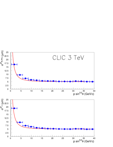
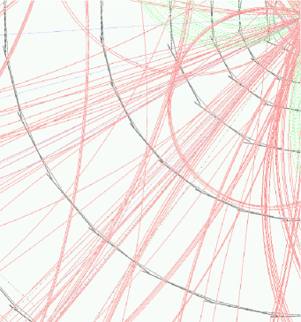
Figure 3.17: Track extrapolation resolution at CLIC. Left: Impact parameter accuracy as function of $p_{t}$ for the $R$–$\phi$ (upper plot) and $R$–$z$ (lower plot) projections. Right: Display of a multijet event simulated with GEANT3 showing secondary decays in $b$ jets.

Pixel sensors of different technologies can be considered, from CCDs to the monolithic pixel sensors of new design currently under development. Potentially interesting technologies and an outline of the needed R&D are discussed later in this section.

Jet-flavour tagging, based on the combination of particle topology and kinematics, has succesfully been applied to experiments at LEP and the SLC. The kinematics in multi-TeV $e^{+}e^{-}$ collisions suggests that the extensions of the reconstruction and tagging algorithms, pioneered at LEP and the SLC and further developed for application at a lower-energy LC, may need to be reconsidered. The high jet collimation and large $b$ decay distance pose significant challenges to the track pattern recognition and reconstruction that may affect the accuracy of $b$ and $c$ identification, relying only on secondary vertex and impact parameter tagging. It is thus interesting to consider new quark tagging techniques, which profit from the kinematics of multi-TeV $e^{+}e^{-}$ collisions. A $b$-tagging algorithm based on the tag of the steps in particle multiplicity originating from the heavy hadron decay along its flight path echoes a technique developed for charm photoproduction experiments [31]. At CLIC, the signal of the production and decay of a $b$ or $c$ hadron can be obtained from an analysis of the number of hits recorded within a cone centred on the jet direction as a function of the radial position of the detector layer. In the tested implementation of the algorithm, a cone of half-aperture angle $\psi$ = 40 mrad, optimized to maximize the sensitivity in the presence of background and fragmentation particles, defines the area of interest (AoI) on each detector layer. The decay of a highly boosted short-lived hadron is characterized by a step in the number of hits recorded in each AoI, corresponding to the additional charged multiplicity generated by the decay products.

Since the average charged decay multiplicity of a beauty hadron is about 5.2 and that of a charm hadron 2.3, the $B$-decay signature can consist of either one or two steps, depending on whether the charm decay length exceeds the vertex tracker layer spacing.

The number of background hits in the AoI is estimated to be 0.7, constant with the radius, the increase of the AoI surface being compensated by the background track density reduction due to the detector solenoidal field. This background density can be monitored, by sampling the region outside the AoI, and subtracted. The effect of significant fluctuations of the number of these background hits and of low-momentum curling tracks in the innermost layers can also be removed. The typical multiplicity pattern of a tagged $B$ decay is shown in Fig. 3.13.

Jets with an upward multiplicity step at least larger than 1 and a total multiplicity increase larger than 2 have been considered. According to the simulation, 69%, 29% and 3% of these jets are due to $b$, $c$ and light quarks respectively. The $b$ jets can be further discriminated using a $b$-likelihood based on the size, radial position and number of multiplicity steps, the fraction of the jet energy and the invariant mass of the tracks originating at the detected multiplicity steps. The resulting likelihood for $b$ and lighter jets and the $b$ efficiency and purity resulting from a cut on this discriminating variable are shown in Fig. 3.18.

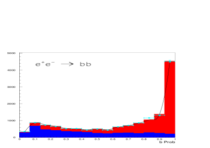
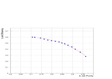
Figure 3.18: The $b$ likelihood for jets in $e^{+}e^{-}\to q\bar{q}$ events at $\sqrt{s}$ = 3 TeV (left) with a multiplicity tag. The response for $b$ ($c$ and lighter) jets is shown in light (dark) grey. The $b$-jet efficiency is given as a function of the purity corresponding to different likelihood cut values (right).

Table 3.9: Average decay distance in space for $B$ hadrons at different $\sqrt{s}$

$\sqrt{s}$ (TeV)	0.09	0.2	0.35	0.5	3.0
Process	$Z^{0}$	$HZ$	$HZ$	$HZ$	$H^{+}H^{-}$   $|$   $b\bar{b}$
$d_{\rm space}$ (cm)	0.3	0.3	0.7	0.85	2.5   $|$   9.0

3.4.4 Main Tracker

Possible concepts for the central tracking device are similar to those studied for the 500 GeV LC, a small silicon tracker surrounded by a large TPC, and for CMS at the LHC, a compact full Si tracker in an intense magnetic field. A TPC would offer some advantages by providing continuous hit information along the charged-particle trajectory, a large lever arm with a minimum material burden, and $dE/dx$ specific ionization information, useful for particle identification. However, local occupancies and two-track separation may represent serious limitations. The total occupancy of a TPC with a inner radius of 50 cm, which integrates a full train due to its maximum drift time of $\simeq$ 50 $\mu$s is estimated to be a few per cent. However, the local track density in hadronic jets is extremely high due to the large boost. Figure 3.19 shows the result of a GEANT3 simulation of $e^{+}e^{-}\to b\bar{b}$ events at $\sqrt{s}$ = 0.5 TeV and 3 TeV with a solenoidal filed of 4 T and 6 T, respectively.

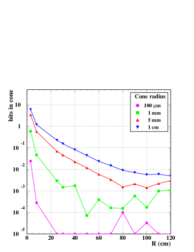
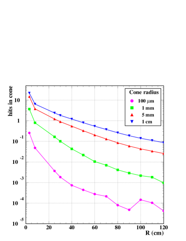
Figure 3.19: Average number of additional hits within a cone of a given radius, as a function of the radius of the tracking layer. Left: $\sqrt{s}~{}=~{}500$ GeV, $B~{}=~{}4$ T; Right: $\sqrt{s}~{}=~{}3$ TeV, $B~{}=~{}6$ T.

The average number of additional hits contained within a cone of given radius around a track hit is plotted as a function of the radial position from the beam line. In the case of 0.5 TeV centre-of-mass energy, the probability to find additional hits within 1 cm distance at a radius of 40 cm is below 10%. However, in the case of multi-TeV collisions, the jet collimation becomes so pronounced that for 1 cm distance a 10% probability for an additional hit is only reached at radii exceeding 1 m. Hence, a solid-state tracker with its intrinsic two-track resolution of 100 $\mu$m seems to be an advantageous option for quality tracking at CLIC. The CMS experiment at the LHC will deploy an all-Si tracker with an active surface of 230 m². While the physics at the LHC and at a 500 GeV LC impose clear requirements on momentum resolution, from processes such as $H\to ZZ\to 4\mu$ and $HZ\to X\mu^{+}\mu^{-}$, at multi-TeV energies there are no obvious benchmark reaction striving for ultimate momentum resolution. A study of the process $e^{+}e^{-}\to\tilde{\mu}\tilde{\mu}\to\mu^{+}\mu^{-}\chi_{0}\chi_{0}$, where the $\tilde{\mu}$ smuon mass is determined from the edges of the muon momentum spectrum, has shown that a momentum resolution comparable to that aimed at for the 500 GeV LC, i.e. $\delta p_{\rm T}/p_{\rm T}^{2}\leq$ 5 $\times$ 10^-5 GeV^-1, seems adequate.

We consider here a central Si tracker consisting of eight concentric layers located between 18 cm and 110 cm from the interaction point. A model of this tracker has been implemented in GEANT3, assuming 0.65% of a radiation length per layer, and is shown in Fig. 3.20. Its performance has been studied with $b\bar{b}$ and $WW$ events. The targeted $\delta p_{\rm T}/p_{\rm T}^{2}\leq$ 5 $\times$ 10^-5 GeV^-1 can be achieved as shown in Fig. 3.20.

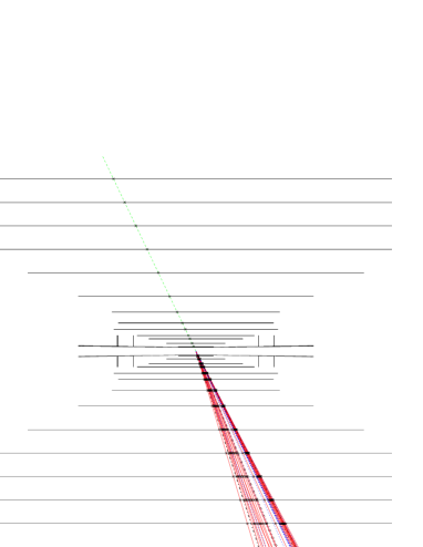
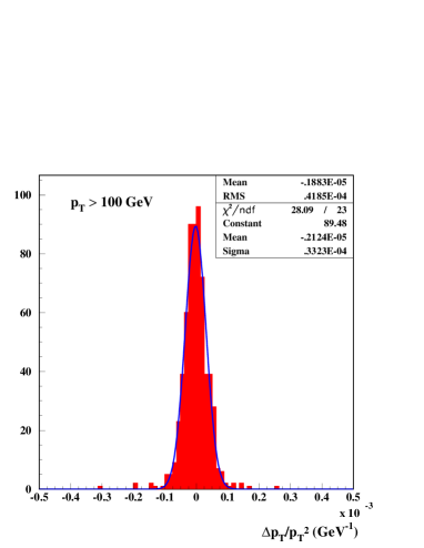
Figure 3.20: The proposed Si tracker for the CLIC detector. Left: $R$–$z$ view of detector layout with a simulated event $e^{+}e^{-}\to W^{+}W^{-}$ at $\sqrt{s}$ = 3 TeV. Right: Momentum resolution for tracks with $p_{T}>$ 100 GeV obtained using the full GEANT3 simulation.

3.4.5 Calorimetry

The quality of the reconstruction of jets at CLIC should be guiding the calorimetry concept. The reasons to achieve the best energy resolution for jets are multiple. A classical example is the need to distinguish hadronic decays of the $Z^{0}$ from those of the $W^{\pm}$, so as to separate the two pair production fusion reactions $e^{+}e^{-}\to Z^{0}Z^{0}\nu\bar{\nu}$ and $e^{+}e^{-}\to W^{+}W^{-}\nu\bar{\nu}$ in the search for possible strong interactions among intermediate vector bosons. The ability to use these hadronic final states besides their leptonic or mixed counterparts would be a key asset in such studies.

Many search channels also claim for a good two-jet mass resolution. The possibility to identify a $Z^{0}$ or a Higgs boson in the final states of supersymmetry is an important tool in deciphering the nature of cascades. Having access to the hadronic modes, such as $h^{0}\to b\bar{b}$, is required to ensure a sizeable event yield.

Another example is the radion search, an object similar to the Higgs bosons whose main decay channel is a pair of gluons. The little Higgs scenario, to be identified, would require a precise measurement of its $W^{3}_{H}$ boson modes into $\ell\bar{\ell}$, $q\bar{q}$ and $Zh$.

A first requirement from the calorimetry would be to avoid the usual weak points (of most systems conceived up to now), namely a break between the electromagnetic sector and the hadronic part, either due to the coil or to some other uninstrumented gap. Since any electromagnetic system has about one interaction length, a large fraction of hadrons interact in its depth and the first interaction is poorly sampled.

It is likely that the way to approach the required performances at CLIC is to achieve the best possible energy-flow reconstruction. The energy-flow technique was developed at LEP and has been adopted for the current LC detector studies. This technique combines tracking and calorimetric information in an optimal way to obtain the best possible resolution on the energy of the produced partons. This requires an optimal distinction between hadrons, neutral and charged, electrons, photons and muons with a minimal double-counting. At CLIC the boost is large enough to make intra-jet particle separation difficult, as exemplified by the energy-flow plot of Fig. 3.21.

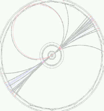
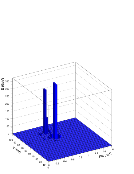
Figure 3.21: A $e^{+}e^{-}\to W^{+}W^{-}$ event at $\sqrt{s}$ = 3 TeV (left) and the energy flowing at the entrance of the e.m. calorimeter located at a radius of 170 cm, assuming a solenoidal field of 6 T and 5 $\times$ 5 cm² cell size (right)

Conventional wisdom and present experience then call, beside other requirements, for high granularity, both transverse and longitudinal, to disentangle neutral energy deposits from those produced by charged particles, which are already accounted for by the more accurate tracker measurements. This requires on the one hand a dense radiator material, with minimal Moliere radius, and a finely segmented readout. On the other hand a sufficiently large radius, with excellent matching between charged particle tracks, as seen in the main tracker and the calorimeter information is needed. Beside having a minimal amount of material along the tracker, this implies that the transition zone, involving the outermost end of the tracker and the front part of the calorimeter should be particularly well studied, with minimal thickness of the inert and minimal albedo effects. The problem may be particularly acute in the forward region, because of the rates and of the effect of interactions in the mask.

Given the time scale and the rapid evolution of techniques, we are still far from having a worked out scenario. On the other hand we advise to define and set up, or join, a strong program of R&D along the lines defined in [32, 33, 34] aiming at a very finely pixellated calorimeter, made of a dense tungsten radiator and a very compact detecting medium, such as silicon. In its main lines this activity should address the modelling of the transition from the main tracker to the calorimeter, understand the merits of a digital approach for the hadronic part with respect to a more classical sampling approach, and whether compensation should be used.

3.4.6 Forward Region

The small-angle environment at CLIC is very demanding for low-angle calorimetry: the region below 50 mrad, in particular, will be difficult to instrument, both because of the high level of radiation and particle density. At larger polar angles the situation improves and we are led to believe that various types of detectors are suited for operating at polar angles above 100 mrad. Simulation results show, however, that there still is a sizeable amount of energy deposited by $\gamma\gamma$ background, between 100 mrad and 400 mrad.

The evaluation of the $\gamma\gamma\to{\mathrm{hadrons}}$ background was performed using the output of the GUINEAPIG simulation. Backgrounds have then been tracked through the detector using the GEANT3 simulation up to scoring planes located at $\pm$150 cm downstream from the interaction region.

The results of the simulation show that the situation is manageable down to 300 mrad for general hadronic events and down to about 100 mrad for identifying and measuring energetic electrons from Bhabha events and from fusion processes such as $e^{+}e^{-}\to ZZe^{+}e^{-}$. Assuming that the forward calorimetric coverage is located at 200 cm from the interaction point, the $\gamma\gamma$ energy would spread over an area of 20 cm radius. Using a small Moliere radius material for the e.m. calorimeter, one should be able to confine showers from high energy electrons to a transverse area about one order of magnitude smaller than the figure reported above. Taking into account that the average energy per particle in $\gamma\gamma$ events is $\simeq$ 2.5 GeV, this contribution does not spoil the energy measurement of a 250 GeV electron.

Even requiring a minimum angle close to 300 mrad, for total energy measurement purposes it is not feasible to integrate a full train. The average deposited energy per $\gamma\gamma$ event at 280 mrad is shown in Fig. 3.22.

Figure 3.22: The average deposited energy for $\gamma\gamma$ event at angles larger than 280 mrad

Timing capability should be implemented up to polar angles of about 400 mrad. Two strategies are available: either to incorporate time-stamping capabilities in the whole forward calorimeter or to break the end-cap calorimeter in two sections. One with nsec-type time resolution and the other extending the same technology as the main calorimeter. A specialized calorimeter at small angle is better optimized and represents the option discussed here.

Small-angle calorimetry for luminosity measurement and beam condition monitoring covers the angular region below 100 mrad. These devices must have good properties for radiation hardness and time resolution. Out of the various options for the active part of this type of calorimeters, one might use diamond, quartz fibers, parallel-plate chambers, liquid scintillators; we focus here on quartz fibers. Such detectors have been widely used in various applications. R&D has been carried out to address the main requirements. Energy resolutions better than 40%/$\sqrt{E}$ have been routinely obtained. The output light is mostly due to Cherenkov effect by high energy particles in the shower. As for the timing characteristics, the Cherenkov light is intrinsically fast and allows resolutions of the order of 1 nsec to be achieved. As noted before, a requirement is for the low-angle calorimeter to have a very small Moliere radius. The choice of lead as radiator imposes small gaps for the quartz fibres, and using these as active medium improves on the already small Moliere radius achieved with lead. In fact the fibres are sensitive to those high-energy particles in the shower which travel close to the original primary trajectory. Such a phenomenon is extremely important for hadronic showers. The shower radius has been found to shrink by a factor of 3 for the same radiator material. The effect is instead a factor of about 2 for e.m. showers. The discrimination of high-energy electrons benefits from this feature. Given the smaller radius, all edge effects will also be of lesser importance. Using a volume ratio of 10:1 gives an equivalent Moliere radius well below 1 cm. This can be further reduced by adopting tungsten as the passive radiator.

3.4.7 Summary of Detector Performance

The parameters and response of the different detector components are summarized in Table 3.10. The tracking performance has been validated using the full GEANT simulation in terms of both momentum resolution and track extrapolation accuracy. The calorimetric performances are derived from those assumed in the TESLA study, as they should not be significantly affected by the larger energy. The coverage is limited in the forward region by the beam delivery system and forward background.

Table 3.10: Summary of detector performances

Detector		CLIC studies
Vertexing		$\delta(IP_{r\phi})=15~{}\mu{\rm m}\oplus{35~{}\mu{\rm m}~{}{\rm GeV}/c\over{p\sin^{3/2}\theta}}$
		$\delta(IP_{z})=15~{}\mu{\rm m}\oplus{35~{}\mu{\rm m}{\rm GeV}/c\over{p\sin^{5/2}\theta}}$
Solenoidal field		B = 4.0 T
Tracking		${\delta p_{t}\over{{p_{t}}^{2}}}$ = 5.0 $\times$ 10-5 ${\left(\frac{{\rm GeV}}{c}\right)}^{-1}$
E.m. calorimeter		${\delta E\over E~{}({\rm GeV})}$ = 0.10 ${1\over\sqrt{E}}\oplus$ 0.01
Hadron calorimeter		${\delta E\over E~{}({\rm GeV})}$ = 0.50 ${1\over\sqrt{E}}\oplus$ 0.04
$\mu$ detector		Instrumented Fe yoke $\frac{\delta p}{p}\simeq$ 30% at 100 GeV/$c$
Energy flow		${\delta E\over E~{}({\rm GeV})}\simeq$ 0.3 $\frac{1}{\sqrt{E}}$
Coverage		$\left|\cos\theta\right|<$ 0.98

3.4.8 Luminosity Measurement and Energy Calibration

The intense beamstrahlung that smears significantly the luminosity spectrum will have to be accurately measured and unfolded from the observed data, to relate them to theoretical predictions. Accurate determinations of both the absolute luminosity and the luminosity spectrum are therefore crucial to preserve the CLIC physics potential. Bhabha scattering $e^{+}e^{-}\to e^{+}e^{-}$ represents a favourable reaction, with a cross section still sizeable beyond 1 TeV (9.4 pb at $\sqrt{s}$ = 3 TeV) and a simple, accurately measurable final state.

3.4.8.1 Luminosity determination with Bhabha scattering

At LEP-1 a final luminosity precision of 0.07% was achieved, by using double-tags for the Bhabha process. The theoretical QED prediction for the Bhabha process at LEP was obtained using the BHLUMI Monte Carlo program [35]. The theoretical uncertainty $\sigma_{\rm th}$ of the BHLUMI prediction was estimated originally to be 0.1% [36], and later reduced to the level of 0.07% [37, 38, 39]. The main contributions to the theoretical uncertainties at LEP-1 were (a) the photonic second-order subleading correction $O(\alpha^{2}L_{e})$ where $L_{e}=\ln\frac{|t|}{m_{e}^{2}}$; (b) the hadronic vacuum polarization; and (c) the $O(\alpha^{2})$ light fermion-pair production. The $s$-channel $Z$ contribution being only $\sim$ 1%, its contribution was well under control. At LEP-1, the measured Bhabha rate had to be substantially larger than that of the $s$-channel $Z$ at the resonance peak. Hence, the polar-angle acceptance was pushed down to 25–50 mrad range, corresponding to $\sqrt{|t|}$ of 1–2 GeV.

At CLIC, the angular range of Bhabha luminometer will need to be shifted to $\sim$ 50–100 mrad due to background conditions. At 3 TeV, the $t$-channel transfer becomes 75–150 GeV and the $t$-channel $Z_{t}$ exchange can in principle be as important as that of the $t$-channel photon exchange $\gamma_{t}$. The contribution from hadronic vacuum polarization increases at higher transfers too. It is thus important to estimate the magnitude of these theoretical uncertainties in the low-angle Bhabha (LABH) process at multi-TeV energies.

The contributions from photonic corrections will scale linearly with $L_{e}$, if some part of $O(\alpha^{2}L_{e})$ will still be missing from the Monte Carlo generators (which is however unlikely by a realistic time for CLIC operation). We therefore estimate the photonic uncertainty to increase, at most, by $\simeq$ 30% w.r.t. its LEP-1 value. The $Z_{t}$ contribution was estimated by completely removing the $Z$ contribution. This changes the cross section by a few 0.1% at 0.8 TeV and by 2–6% at 3 TeV.

The theoretical uncertainty of the $O(\alpha)$ electroweak corrections in the LABH process at CLIC have been estimated with the help of the DIZET EW library of ZFITTER [40, 41]. This was obtained by manipulating the non-leading $O(\alpha^{2})$ EW corrections of $O(G_{F}^{2}M_{t}^{2}M_{Z}^{2})$ of Degrassi et al., keeping $O(G_{F}^{2}M_{t}^{4})$ as accounted for. This is shown in Fig. 3.23, where the effect of change of $M_{H}$ from 120 GeV to 500 GeV is also given. We estimate them to be 0.025% at 0.8 TeV and 0.10% at 3 TeV. Changing $M_{t}$ from 165 GeV to 185 GeV has led to even smaller effect. In summary, $\sigma_{\rm th}\simeq$ 0.10% of the LABH luminometer at CLIC because of EW corrections emerges as a conservative estimate.

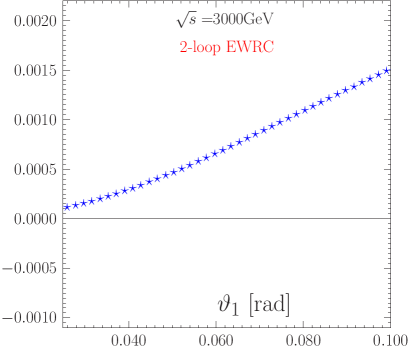
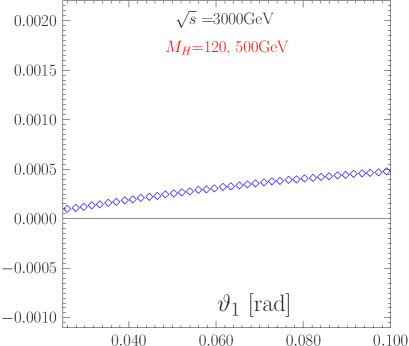
Figure 3.23: Change of Bhabha differential cross section due to uncontrolled 2-loop corrections and due to Higgs mass error. Results were obtained using the DIZET library of ZFITTER [40, 41].

The theoretical uncertainties of LABH due to hadronic vacuum polarization (HVP), taking 1995 estimates of HVP of Refs.[42, 43], was estimated as 0.03% at LEP-2. Using the same calculation of HVP we get 0.12% at 3 TeV, i.e. larger by a factor of 4. This means that HVP would become the dominant component of theory systematics on the absolute luminosity at CLIC. However, the recent improvements of HVP [44, 45] modifies the situation substantially: according to preliminary estimates we get a factor 2 reduction in the error due to HVP. By the time of CLIC operation, we hope for another factor 2 of improvement.

Summarizing, we think that a theoretical uncertainty $\sigma_{\rm th}\simeq$ 0.1% for the low-angle Bhabha process at energies up to 3 TeV is realistic.

Since the LABH cross section depends as 1/$s$ on the total CMS energy, in order to preserve the 0.1% precision of LABH, a knowledge of the absolute beam energy calibration to $\sim$ 0.05% accuracy is needed. The energy spectrum of the luminosity also needs to be determined, which can be obtained accurately using the acolinearity of Bhabha scattering as discussed in the next section.

3.4.8.2 Bhabha scattering and $\sqrt{s^{\prime}}$

The reconstruction of the effective $e^{+}e^{-}$ energy $\sqrt{s^{\prime}}$ from the acolinearity in large-angle Bhabha events has been proposed for a lower energy linear collider [46], extending the experience with the $\sqrt{s^{\prime}}$ determination at LEP-2 [47].

In the approximation where the energy lost before the $e^{+}e^{-}$ interaction is radiated in a single direction, the effective collision energy $\sqrt{s}$ can be related to the final state $e^{+}e^{-}$ acolinearity by

$$\sqrt{s^{\prime}}=\sqrt{s}\sqrt{1-2\frac{\sin(\theta_{1}+\theta_{2})}{\sin(\theta_{1}+\theta_{2})-\sin\theta_{1}-\sin\theta_{2}}}\,,$$

where $\theta_{1}$ and $\theta_{2}$ are the angles of the final electron and the positron w.r.t. the photon direction. Therefore, with this assumption, the $\sqrt{s^{\prime}}$ distribution can be measured by a determination of the $e^{+}$ and $e^{-}$ directions. At CLIC, there are two main processes leading to electron and positron energy loss, beamstrahlung (BS) and initial-state radiation (ISR). In order to infer the $\sqrt{s^{\prime}}$ spectrum due to BS, it is important that ISR can be reliably computed and unfolded from the measured distribution.

A preliminary study has been performed by generating Bhabha events with the BHLUMI 4.04 generator [35]. The CLIC electron and positron energy spectra have been obtained from the result of the beam simulation for the CLIC parameters at 1.5 TeV beam energy and the effect of the beam energy spread in the Linac has been included in the form of a Gaussian smearing with a r.m.s. of 6 GeV. The determination of $\sqrt{s^{\prime}}$ has been based only on the electron and positron direction determination, assuming a tracking coverage down to $7^{\circ}$ in polar angle. While the calorimetric information may provide further important constraints, it needs to be validated by a full simulation, accounting for the background conditions at small angles. Therefore, no attempt to reconstruct ISR photons has been made in this study. It is also important to measure the final-state-particle energy so as to be able to disentangle the effect of the correlations in the energies of the colliding particles, which are not taken into account in the approximation introduced.

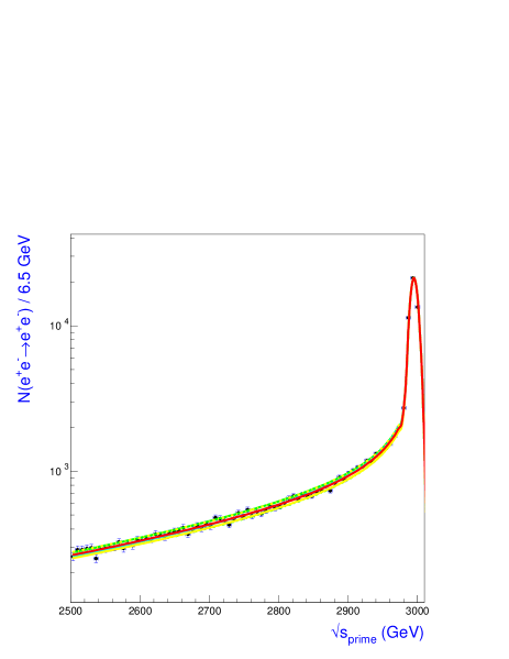
Figure 3.24: The reconstructed luminosity spectrum for CLIC at 3 TeV (points with error bars). The continuous lines represent the fit obtained using the first of the parametrizations discussed in the text, for the fitted value and by varying the parameters within the $\pm$ 2 $\sigma$ range.

The beamstrahlung spectrum has been parametrized using two models: 1) the modified Yokoya–Chen approximation [48]: $e^{-N_{\gamma}}\big{(}\delta(x-1)+\frac{e^{-k(1-x)/x}}{x(1-x)}h(x)\big{)}$, $h=f(\Upsilon)$ where $N_{\gamma}$ and $\Upsilon$ are treated as free parameters, and 2) the CIRCE polynomial form: $a_{0}\delta(1-x)+a_{1}x^{a_{2}}(1-x)^{a_{3}}$ were the free parameters are $a_{0}$, $a_{2}$, $a_{3}$, respectively. The fraction $F$ of events outside the 0.5% of the nominal $\sqrt{s}$ energy has also been left free and extracted from the reconstructed data.

The accuracy on the parameters has been obtained by performing a likelihood fit to the reconstructed $\sqrt{s^{\prime}}$ spectrum and the uncertainty on the mean $\sqrt{s^{\prime}}/\sqrt{s}$ has been extracted accounting for correlations. The results are given in Table 3.11 for an equivalent luminosity $\int{\cal{L}}$ = 15 fb^-1, corresponding to $\simeq$ 3 days at the nominal luminosity of $10^{35}$ cm^-2s^-1. The study has been performed for two different assumptions on the CLIC parameters, denoted here as CLIC.01 and CLIC.02, corresponding to different beamstrahlung spectra.

Table 3.11: The relative accuracy for the parameters in the Yokoya–Chen and CIRCE parametrization

Parameter		CLIC.01	CLIC.02
$\delta N_{\gamma}/N_{\gamma}$		$\pm$ 0.044	$\pm$ 0.084
$\delta\Upsilon/\Upsilon$		$\pm$ 0.019	$\pm$ 0.018
$\delta\sqrt{s^{\prime}}/\sqrt{s}$		$\pm$ 7.8 $\times$ 10-5	$\pm$ 5.3 $\times$ 10-5
$\delta a_{0}/a_{0}$		$\pm$ 0.044	$\pm$ 0.049
$\delta a_{2}/a_{2}$		$\pm$ 0.089	$\pm$ 0.058
$\delta a_{3}/a_{3}$		$\pm$ 0.018	$\pm$ 0.021
$\delta\sqrt{s^{\prime}}/\sqrt{s}$		$\pm$ 9.8 $\times$ 10-5	$\pm$ 7.2 $\times$ 10-5

The sensitivity to details of the beamstrahlung spectrum obtained in this analysis needs to be further validated once the detector resolution effects have been taken into account. However it has been shown that the detector resolution can be made small with respect to the intrinsic beam energy spread.

3.5 Simulation Tools

The influence of backgrounds on the extraction of physics signals cannot be forgotten. Tools have thus been developed to account for these effects by overlaying background particles to physics events and by simulating the $\sqrt{s}$ energy smearing effects due to the beamstrahlung. These tools are interfaced to the simulation programs used in the physics analyses discussed in the second part of this report. The detector response has been incorporated both through full GEANT3 simulation and through a parametric smearing program. Both are based on the software developed in the framework of the ECFA/DESY Workshops on Physics and Detectors at a $e^{+}e^{-}$ Linear Collider, but have been customized to describe the CLIC specific geometry and detector concept.

3.5.1 BDSIM

A detailed simulation program BDSIM [6] has been developed, based on GEANT4 [49], to model the beam delivery system (BDS). BDSIM builds the BDS GEANT4 geometry directly from an accelerator (MAD) optics file, which allows a rapid turn-around as the BDS designs get updated. BDSIM incorporates efficient accelerator-style tracking based on transfer matrix techniques, together with the standard shower generation and physics processes of GEANT4. The program has been used to study electron/positron tracking, collimation, muon production  [50, 51], and the backgrounds associated with secondaries from showers produced when primary beam or halo particles strike apertures along the BDS. BDSIM also allows for specialized processes such as the tracking of Compton-scattered electrons and photons from a laser-wire  [52], including the effects of backgrounds and limitations of beam line apertures. Such a study was first performed for the nominal long CLIC 1.5 TeV BDS [8]. BDSIM continues to be upgraded and now also incorporates hadronic processes, including neutron production and tracking. GEANT4 is set up to allow for efficient weighting and biasing of events and tracks, and BDSIM will incorporate these techniques to provide high-statistics background estimates for physics and detector studies as well as for BDS optimization. It is also planned to interface BDSIM directly to the next generation of detector simulation codes as they are developed.

3.5.2 GUINEAPIG

The GUINEAPIG code simulates the beam–beam interaction in a linear collider. It was originally developed for TESLA [16] and later extended to be able to simulate CLIC at high energies [17]. The program uses a clouds-in-cells method to calculate the effect of the fields of one beam on the incoming beam. A beam is typically represented by about 10⁵ macroparticles. The emission of beamstrahlung is simulated by approximating the particle trajectory locally with a circular motion and using the Sokolov–Ternov spectrum [53] for the radiation. The produced photons are also tracked on the grid. The production of coherent pairs from the beamstrahlung photons is implemented similarly to the beamstrahlung. It is also possible to load an arbitrary distribution of particle from an input file, so as to be able to take full advantage of the simulation of other components of the accelerator.

The production of incoherent pairs, bremsstrahlung and hadronic background, is achieved using the Weizäcker–Williams approach. Each beam particle is replaced by a number of virtual photons. In the collision these photons are treated as real and the cross sections for $\gamma\gamma\to e^{+}e^{-}$ and $\gamma\gamma\to hadrons$ are used. Secondary electrons and positrons are tracked through the field of the beams. Beam-size effects and those due to the strong field on the virtual photon spectrum can also be taken into account [16].

The produced particles and the beams can be saved after the simulation and so used for further studies. Also the collision energies of electrons, positrons and photons can be stored allowing the reconstruction of the luminosity spectra, including all correlations. The CALYPSO and HADES program libraries provide useful tools for interfacing with event generation and detector simulation programs, using the GUINEAPIG outputs.

3.5.3 CALYPSO

CALYPSO [54] is a small Fortran library that gives access to the luminosity output files from the GUINEAPIG simulation. An initialization routine allows the file name to be specified and the type of particles to be considered for each beam. Subsequent calls of the main subroutine return the energies of colliding particles. The use of the luminosity file allows the inclusion of the full correlations between the colliding beams. Luminosity data files exist for different energies and can be found in Ref. [54].

There also exists a simple Fortran package that uses parametrizations to generate the energies of colliding particles at $3{\,\rm~{}TeV}$. While the correlation is only partially included and some simplifications are made for the energy spread of the colliding beams, the program reproduces the luminosity spectra quite accurately. This library needs no data files but must be linked to the CERN library CERNLIB.

3.5.4 HADES

HADES consists of two parts. The first is a simple Fortan library that can write and retrieve background events to and from a file. Originally designed for hadronic background, the library allows the generation of background events with any generator and their storage in a file. With other routines, it is easy to randomly choose a number of events from such a file and add to them an event generated with PYTHIA. HADES has been used in these studies also to load and overlay the muon background. The second part is a small program that uses PYTHIA to generate the hadronic background events from the initial photons provided by GUINEAPIG. Hadronic background files exist for CLIC at $E_{c.m.}$ = 3  TeV and $E_{c.m.}$ = 5 TeV [19].

3.5.5 GEANT Simulation

A full simulation of the CLIC tracking system has been developed, based on GEANT3 and on the BRAHMS program set up for the TESLA study. In the CLIC version, the beam-pipe configuration and the tungsten-mask geometry have been modified accordingly and a multilayered tracker based on Si sensors has been implemented according to the conceptual design discussed above. The GEANT program has been interfaced with CALYPSO and HADES to include the beamstrahlung effects and overlay backgrounds. The pair, $\gamma\gamma\to hadrons$ and parallel muon backgrounds have been implemented and used in the studies. The GEANT program has been used both to provide parametrizations of the tracking performances used in the fast simulation and to carry out analyses based on the tracker only such as the development of the $b$-tagging algorithm discussed above and the smuon pair production. For this the track-reconstructed parameters have been passed to the analysis code via the VECP commons in the VECSUB package, so that the same code could be used on the full and fast simulations.

3.5.6 Parametric Detector Simulation

The program SIMDET simulates the reconstruction of $e^{+}e^{-}$ collision events, based on a parametrized detector response. This response was originally tuned on that expected for the TESLA detector, according to its full GEANT3 simulation. For its application to the CLIC studies, several extensions have been implemented . The response has been modified to reflect that expected for a detector suitable for use at CLIC. The track momentum resolution and extrapolation accuracy have been parametrized according to the results of the full GEANT3 simulation of a discrete multilayered Si tracker. Also the angular coverage has been modified, while the calorimeter performances have been kept as for the TESLA detector.

SIMDET provides a fast treatment of detector simulation and event reconstruction, while ensuring rather realistic performances. The basic detector components implemented are:

• Vertex tracker,

• Main tracker and Forward tracker,

• Electromagnetic calorimeter,

• Hadronic calorimeter

• Low-angle tagger and low-angle luminosity calorimeter.

The program applies Gaussian smearing to charged-particle momenta and impact parameters with resolutions obtained from full simulation. The calorimetric response is also treated parametrically. Pattern recognition is emulated by means of cross-reference tables between generated particles and detector response. An energy-flow algorithm defines the output of the program. The track covariance matrix and $dE/dx$ information is also available.

SIMDET processes events generated in line with PYTHIA, and also events stored in HepEvt format. As part of the CLIC extensions, an interface with partons generated with the CompHep program has been set up. It is thus possible to read CompHep event files and perform hadronization and short-lived particle decays in line. Also, the CALYPSO and HADES interfaces have been added to read the luminosity spectrum and overlay backgrounds, respectively. In the CLIC physics studies, the GUINEAPIG luminosity files have been used to describe the shape of the luminosity spectrum and to overlay the $\gamma\gamma\to hadrons$ and the parallel muon backgrounds.

After simulation, particles are classified, for the purpose of physics analysis, as electrons, photons, muons, charged hadrons (taken as pions), neutral hadrons (taken as long-lived kaons) and clusters of unresolved particles. Detector coverage, tracking efficiencies, charge mismeasurement and threshold energies for detector response are taken into account with user-adjustable values. These have been tuned according to the CLIC detector concept discussed earlier on.

Best estimates for energy-flow objects have been stored using the VECSUB conventions and used for the physics analyses.

3.6 Generators and Physics Code

3.6.1 Monte Carlo Event Generators for CLIC

Monte Carlo (MC) event generators are an essential tool in all experimental analyses. In this section we will briefly recall the key features of these programs and describe those simulations which are available for CLIC physics. Here we limit ourselves to the discussion of the physics event generators. These programs must be interfaced to both detector simulations and beam energy spectra in order to give a complete simulation. In general the MC event generation process can be divided into three main phases: (1) The hard process where the particles in the hard collision and their momenta are generated, usually according to the leading-order matrix element. (2) The parton-shower phase where the coloured particles in the event are perturbatively evolved from the hard scale of the collision to the infrared cut-off. The emission of electromagnetic radiation from charged-particles can be handled in the same way. (3) A hadronization phase in which the partons left after the perturbative evolution are formed into the observed hadrons.

Most generators fall into one of two classes: general-purpose event generators aim to perform the full simulation of the event starting with the hard process and finishing with the final-state hadrons; the second class of programs perform only the hard scattering part of the simulation and rely on one of the general-purpose generators for the rest of the simulation.

During the LEP era the most common practice was to rely on the general-purpose Monte Carlo programs for the description of hadronic final states supplemented with more accurate parton-level generators interfaced to general-purpose event generators for specific processes, for example four-fermion production. At future linear colliders, and particularly CLIC, this is even more important as we wish to study final states with higher multiplicities, for example six or even eight fermions, which cannot be described by the general-purpose generators.

We will first discuss the general-purpose event generators. This is followed by a discussion of the parton-level programs that are available to calculate particular final states and the automatic programs that are available to calculate any final state.

3.6.1.1 General-purpose event generators

Historically the main general-purpose generators have been HERWIG [55], ISAJET [56], and PYTHIA [57]. While the general philosophy of these programs is similar, the models used and approximations made are different. In general, at least for $e^{+}e^{-}$ collisions, the range of hard production processes available in the different generators is very similar. All the generators have a wide range of SM processes predicted by the MSSM, and some processes for other models.

The differences in the parton shower phase of the process are more pronounced. While ISAJET still uses the original parton-shower algorithm which only resums collinear logarithms, both HERWIG and PYTHIA include the effects of soft logarithms via an angular-ordered parton shower in the case of HERWIG and by applying a veto to enforce angular ordering on a virtuality-ordered shower in the case of PYTHIA. There is also a separate program, ARIADNE[58], which implements the dipole cascade and is interacted to PYTHIA for hadronization. Like the parton-shower phase the models used for the hadronization phase are very different in the different programs. ISAJET uses the Feynman-Field independent fragmentation model while PYTHIA uses the LUND string model and HERWIG the cluster hadronization model.

While these programs will continue to be used in the near future, a major programme is under way to produce a new generation of general-purpose event generators in C++. The main aim of this programme is to provide the tools needed for the LHC. However, these tools will be used for the next generation of linear colliders. The only generator currently available in C++ that can generate physics results is APACIC++[59]; work is under way to rewrite both PYTHIA [60] and HERWIG [61] in C++. These programs should be available in the next few years and we expect them to be the major tools for event generation at CLIC.

3.6.1.2 Parton level programs

Many programs are available to calculate an individual hard process, or some set of hard processes, and are interfaced to one of the general-purpose generators, most often PYTHIA, to perform the parton shower and hadronization. In this brief review it is impossible to list all these programs and discuss them.

As many of these programs were used by the LEP collaborations, a detailed discussion of both two- [62] and four- [63] fermion generators can be found in the report of the LEP-II Monte Carlo workshop [64]. In addition there is also one program, LUSIFER [65], for six-fermion processes. In practice the computation of processes with six or more final-state particles is complex and it seems likely that these calculations will be performed by the automatic programs discussed in the next section.

3.6.1.3 Automatic matrix element calculations

There are an increasingly large number of programs available that are capable of calculating and integrating the matrix elements for large numbers of final-state particles automatically.

In general there are two important components of any such program. The first step is the calculation of the matrix element for a given momentum configuration. There are three different techniques in use to perform this step of the calculation: (1) The matrix element squared can be evaluated symbolically using traditional trace techniques. (2) A number of programs use helicity amplitude techniques to evaluate them. (3) There are techniques [66] which can be used to evaluate the matrix element without using Feynman diagrams.

The second step of the process is to integrate the matrix element. There are two main techniques in use: One approach is to use adaptive integration programs such as VEGAS [67] to perform the integration. A second approach is to use the knowledge of the matrix element to perform multi-channel phase-space integration based on its peak structure.

In practice some programs combine these two approaches. In general, adaptive programs such as VEGAS [67] are ill-suited to the integration of functions which have complex peaked structures, such as multiparticle matrix elements, and therefore for most practical applications multichannel integration techniques converge much faster.

There are a number of programs available which combine a variety of these techniques:

1. AMEGIC++ [68] makes use of helicity amplitude techniques to evaluate the matrix element together with efficient multichannel phase-space integration to calculate the cross section.

2. CompHep [69] is an automatic program for calculation of the cross section for processes with up to eight external particles. It uses the traditional trace techniques to evaluate the matrix element together with a modified adaptive integrator to compute the cross section.

3. GRACE [70] combines the calculation of matrix element via helicity amplitude techniques and adaptive integration to calculate cross sections. Recently it has been used to calculate the one-loop corrections to Higgs production in $WW$ fusion [71].

4. HELAC/PHEGAS uses the approach of Ref. [72] which is based on the Dyson–Schwinger equation together with multichannel integration [73] to calculate the cross section.

5. MADGRAPH/MADEVENT [74] uses helicity amplitude techniques for the matrix element together with an efficient multichannel phase-space integrator to compute the cross section.

6. WHIZARD is a multichannel integration package which can use either CompHep, MADGRAPH or OMEGA [75] to calculate the matrix elements.

7. There are tools which are used to calculate loop processes [76]: FeynArts automatically generates the Feynman diagrams for the considered process, while FeynCalc evaluates analytically the relevant amplitudes. Another package FormCalc can also be used for the calculation of the loop amplitudes with the numerical evaluation performed by the program LoopTools. All these programs have been also used recently to evaluate the radiative corrections to $e^{+}e^{-}\to H\nu_{e}\bar{\nu}_{e}$ in the SM [77].

All of these programs apart from HELAC/PHEGAS are publicly available. At present only CompHep and GRACE include supersymmetric processes, although the both MADGRAPH and AMEGIC++ can be extended to add the additional interactions which are needed. In order to simulate events these programs needed to be interfaced to the general-purpose event generators. Most of these programs are interfaced to one of the major general-purpose event generators although the details vary from program to program.

3.6.2 Programs for Spectra, Decay and Production

3.6.2.1 Programs for the MSSM spectrum

It is well known that in the unconstrained MSSM, it is a rather tedious task to deal with the basic parameters of the Lagrangian and to derive in an exhaustive manner their relationship with the particle masses and couplings. This is mainly due to the fact that in the MSSM, despite its minimality, there are more than one hundred new parameters. Even if one constrains the model to have a viable phenomenology, there are still more than 20 free parameters left. This large amount of input enters in the evaluation of the masses of $O$(30) SUSY particles and Higgs bosons as well as their complicated couplings, which involve several non-trivial aspects. The situation becomes particularly difficult if one aims at rather precise calculations and hence attempts to include some refinements such as higher-order corrections, which for the calculation of a single parameter need the knowledge of a large part of the spectrum.

However, there are well-motivated theoretical models where the soft SUSY-breaking parameters obey a number of universal boundary conditions at the high (GUT) scale, leading to only a handful of basic parameters. This is the case for instance of the minimal Supergravity model (mSUGRA) and anomaly (AMSB) or gauge mediated (GMSB) SUSY-breaking models. However, this introduces another complication since the low-energy parameters are to be obtained through renormalization group equations (RGE) and the models should necessarily give radiative electroweak symmetry-breaking (EWSB). The implementation of these two ingredients poses numerous non-trivial technical problems when done in an accurate way; this complication has to be added to the one from the calculation of the particle masses and couplings with radiative corrections (RC) which is still present.

To deal with the supersymmetric spectrum in all possible cases, one needs very sophisticated programs to encode all the information and, eventually, to pass it to other programs or Monte Carlo generators to simulate the physical properties of the new particles, decay branching ratios, production cross sections at various colliders, etc. These programs should have a high degree of flexibility in the choice of the model and/or the input parameters and an adequate level of approximation at different stages, for instance in the incorporation of the RGEs, the handling of the EWSB and the inclusion of radiative corrections to (super)particle masses, which in many cases can be very important. They should also be reliable, quite fast to allow for rapid comprehensive scans of the parameter space, and simple enough to be linked with other programs.

There are four main public codes (there are also some private codes which will not be discussed here; see later) which make rather detailed calculations of the Supersymmetric particle spectrum in the MSSM or in constrained scenarios (mSUGRA, etc.):

1. ISASUSY [56], which is available since the early 90s and is implemented in the Monte Carlo generator ISAJET; it is the most widely used for simulations in the MSSM.

2. SuSpect [78], a new version has been released very recently but a preliminary version of the program has existed 1998 and was described in Ref. [79].

3. SOFTSUSY [80], a code written in object–oriented C++ but which has a Fortran interface for calculations in mSUGRA; it was released two years ago.

4. SPHENO [81], which was released this year and also calculates the decay branching ratios and the production rates in $e^{+}e^{-}$ collisions of SUSY particles.

The codes have different features in general, but they all incorporate the four main ingredients or requirements for any complete calculation of the SUSY spectrum: i) the RG evolution, ii) the implementation of radiative EWSB, iii) the calculation of the masses of the Higgs and SUSY particles, including the radiative corrections, and iv) the possibility of performing some checks of important theoretical features and some experimental constraints.

The radiative corrections are particularly important, as is well known, in the Higgs sector. Codes such as ISASUSY and SuSpect have their own approximate calculations, but they are also linked with routines which do a more sophisticated job. The main available routines for the Higgs sector are: Subhpole (SUBH) [82] which calculates the leading radiative corrections in the effective potential approach with a two-loop RG improvement; HMSUSY (HHH) [83] which calculates the one-loop corrections in the effective potential approach and includes the leading two-loop standard QCD and EW corrections; FeynHiggsFast [84], which calculates the corrections in the Feynman diagrammatic approach with the one and two-loop QCD corrections at zero momentum transfer (the version FeynHiggs [85] has the full one-loop corrections and is slower); and BDSZ [86] gives the leading one-loop corrections from the third-generation (s)fermion sector as well as the full $\alpha_{s}\lambda_{t}^{2},\lambda_{t}^{4}$ and $\alpha_{s}\lambda_{b}^{2},\lambda_{t}\lambda_{b}$ corrections at zero-momentum transfer and also has the corrections to the effective potential. The radiative corrections to the SUSY spectrum are in general performed following Pierce, Bagger, Matchev and Zhang [87].

Detailed comparisons of these codes have been performed. The main conclusion is that despite the different ways in which the various items discussed above are implemented, they in general agree at the per cent level in large parts of the MSSM parameter space. Several more important differences occur, however, in some areas of the parameter space, in particular in the high $\tan\beta$ and/or focus point regions with large $m_{0}$ values, where the Yukawa couplings of top and bottom quarks play an important role; see Ref. [88] for details.

3.6.2.2 Decay and production

For the production of SUSY and Higgs particles, the matrix elements of most important processes are already included in the MC generators. However, in some cases, specific-purpose programs which include some higher-order effects such as radiative corrections, spin correlations, width effects, etc. are very useful. A non-exhaustive list of available public codes for Higgs and sparticle production in $e^{+}e^{-}$ collisions including higher-order effects is:

1. SUSYGEN [89] for Higgs and sparticle production, also a MC generator (see above).

2. HZHA [90]: the most used Monte Carlo generator for Higgs production at LEP2.

3. HPROD [91]: a code which calculates the cross sections for SM and MSSM Higgs production in $e^{+}e^{-}$ collisions in the main production channels.

4. SPHENO [81]: discussed earlier and which also calculates the cross sections for SUSY particle production at $e^{+}e^{-}$ colliders.

5. Many four- or six- fermion production processes at $e^{+}e^{-}$ colliders as discussed earlier; some of them have been discussed for the LEP–II MC Workshop [64].

The decays of SUSY and Higgs particles can be rather complicated and it is important to determine them with good accuracy. There can be a large number of decay modes for some particles: simple two-body decays in which it is important sometimes to include higher-order corrections (as is the case for Higgs bosons and strongly interacting sparticles), and rather complicated many-body decay modes such as the three- or four- body decays of charginos, neutralinos and top squarks or important loop-induced decay modes. There are several available codes doing this job with a different level of sophistication:

1. ISASUSY [56]: only tree-level two-body Higgs and SUSY decays (three-body for gauginos).

2. HDECAY [92]: SM and MSSM Higgs decays with higher-order effects.

3. SDECAY [93]: sparticle decays including higher-order effects (RC and multi-body).

4. SPHENO [81]: discussed above and has two- and three-body SUSY particle decays.

Some decay routines are also included in the Monte Carlo event generators SUSYGEN [89], HZHA [90], PYTHIA [57] and HERWIG [55] with possible links to the programs mentioned above. The treatment of SUSY production and decay in the various programs is very different. Both ISAJET and PYTHIA assume that the production and decay of the SUSY particles takes place independently, while HERWIG and SUSYGEN [89] include correlations between the production and decay. HERWIG includes these correlations in all processes [94] while in SUSYGEN they are only included for some processes and decays. Some development in this subject is expected in the near future.

3.7 Standard Model Cross Sections

In order to maximize the sensitivity to new physics signals, it is important not only to consider radiative corrections to the process under investigation, but also radiative corrections to so-called background processes provided by the Standard Model. At multi-TeV energies, some processes are of major interest not only for direct searches, but also as backgrounds for new physics. This is especially true for gauge-boson and fermion-pair production. Electroweak one-loop corrections are a central building block in any precision study of fermion-pair production. The complete set of electroweak contributions, including real hard-photon corrections needs then to be calculated [95, 65]. One novelty at CLIC is that electroweak radiative corrections become sizeable at multi-TeV energies, due to the appearance of Sudakov logarithms. In this section, we first describe the general status of these large corrections, and then discuss the specific reaction $e^{+}e^{-}\to{\bar{t}}t$.

3.7.1 Electroweak Sudakov Logarithms

At the next generation of linear colliders with centre-of-mass energies in the TeV range, well above the electroweak scale, one enters the realm of large perturbative corrections. Even the effects arising from weak corrections are expected to be of the order of 10% or more [96, 97, 98, 99, 100, 101], i.e., just as large as the well-known electromagnetic corrections. In order not to jeopardize any of the high-precision studies at these high-energy colliders, it is indispensable to improve the theoretical understanding of the radiative corrections in the weak sector of SM. In particular this will involve a careful analysis of effects beyond first order in the perturbative expansion in the (electromagnetic) coupling $\,\alpha=e^{2}/(4\pi)$.

The dominant source of radiative corrections at TeV-scale energies is given by logarithmically enhanced effects of the form $\,\alpha^{n}\log^{k}(m^{2}/s)\,$ for $\,k\leq 2n$. These large logarithms arise when the finite particle mass $m$, which is well below the collider energy $\sqrt{s}$, acts as a natural cut-off of a singularity. To give a numerical example, at a collider energy of 1 TeV, logarithmically enhanced $W$-boson corrections of the form $\,\alpha\log^{2}(M_{{}_{W}}^{2}/s)\,$ and $\,\alpha\log(M_{{}_{W}}^{2}/s)\,$ amount to 19% and –4%, respectively. A natural way of controlling the theoretical uncertainties therefore consists in a comprehensive study of these large logarithms, taking into account all possible sources. One class of large logarithms is of ultraviolet origin. They involve short-distance scales and are controlled by the renormalization-group equations. The remaining large logarithms are of soft and/or collinear origin. They involve long-distance scales and, based on QCD/QED experience, they are expected to possess specific factorization properties. Here we review our present understanding of the latter class of large-logarithmic effects.

The potentially most important electroweak corrections are the so-called Sudakov logarithms $\,\propto\alpha^{n}\log^{2n}(M^{2}/s)$, arising from the exchange of collinear-soft, effectively on-shell transverse gauge bosons [102]. It should be noted, however, that for pure fermionic final states (numerical) cancellations can take place between leading and subleading logarithms [103]. For on-shell bosons in the final state, the Sudakov logarithms in general tend to be dominant [97, 101].

Over the last few years, various QCD-motivated methods have been applied to predict the electroweak Sudakov logarithms to all orders in perturbation theory [104, 105, 106]. The methods vary in the way that the QCD-motivated factorization and exponentiation properties are translated to the electroweak theory. This is caused by the fact that the electroweak theory is a spontaneously broken theory with two mass scales in the gauge-boson sector, whereas QCD is basically a single-scale theory. The main debate has therefore focused on the question to what extent the SM behaves like an unbroken theory at high energies.

In Ref. [107] a first hint was given that the transition from QCD to electroweak theory does not come without surprises. It was shown that the Bloch–Nordsieck cancellation between virtual and real collinear-soft gauge-boson radiation [108] is violated for $W$ bosons in the SM as soon as initial- or final-state particles carry an explicit weak charge (isospin) and summation over the partners within an $SU(2)$ multiplet is not performed. In the case of final-state particles the event-selection procedure might (kinematically) favour one of the partners within the $SU(2)$ multiplet, leading to a degree of ‘isospin-exclusiveness’. In the initial state the situation is more radical. At an electron–positron collider the weak isospin of the initial state particles is fixed by the accelerator, in contrast to QCD where confinement forces average over initial colour at hadron colliders. As a result, the Bloch–Nordsieck theorem is in general violated for left-handed initial states, even for fully inclusive cross sections. If we start off with a pure left-handed electron beam, $W$-boson radiation will change this before the actual (hard) scattering process takes place into a mixture of left-handed electrons and neutrinos, with relative weights

$$W_{e_{L}}=\frac{1}{2}\,\Bigl{\{}1+\exp[-2L_{W}(s)]\Bigr{\}}\qquad\mbox{and}\qquad W_{\nu_{e}}=\frac{1}{2}\,\Bigl{\{}1-\exp[-2L_{W}(s)]\Bigr{\}}\,,$$ (3.1)

respectively. The Sudakov coefficient $L_{W}(s)$ is given by

$$L_{W}(s)=\frac{\alpha}{4\pi\sin^{2}\theta_{\rm w}}\,\log^{2}(M_{{}_{W}}^{2}/s)\,,$$ (3.2)

with $\,\theta_{\rm w}\,$ being the weak mixing angle. The difference in the weights originates from the fact that the isospin-singlet component of the beam receives no Sudakov corrections, whereas the isospin-triplet component is subject to the Sudakov reduction factor $\,\exp[-2L_{W}(s)]$. The exponent of this reduction factor amounts to roughly $-0.13$ at $\sqrt{s}~{}=~{}1$ TeV. This implies a 6% neutrino component of the beam at that energy. Since the (hard) scattering cross section can be quite different for left-handed electrons and neutrinos, the corrections due to this electroweak phenomenon can be very large, exceeding the QCD corrections for energies in the TeV range. They are such that at infinite energy the weak charges will become unobservable as asymptotic states [107], which implies for instance an $SU(2)$ charge averaging (‘pre-confinement’) of the initial-state beams.

With this in mind, explicit calculations of (virtual) Sudakov corrections at the two-loop level have been performed to resolve any ambiguity in the translation from QCD to the SM. In the first few calculations, the focus was on pure fermionic processes, like $\,e^{+}e^{-}\to f\bar{f}\,$ [109] and fermion-pair production by an $\,SU(2)\times U(1)$-singlet source [110, 111]. The survey was finally completed by an (Coulomb-gauge) analysis that covered all SM particles [112], including scalar particles as well as transverse and longitudinal gauge bosons. By means of this explicit calculation it was established to what extent the SM behaves like an unbroken theory at high energies.

It was observed that the SM behaves dynamically like an unbroken theory in the Sudakov limit, in spite of the fact that the explicit particle masses are needed at the kinematical (phase-space) level while calculating the Sudakov correction factors. For instance, a special version of the Equivalence Theorem was obtained, which states that the longitudinal degrees of freedom of the massive gauge bosons can be substituted by the corresponding Goldstone-boson degrees of freedom without the need for finite compensation factors. As a result, the Sudakov form factors for longitudinal gauge bosons exhibit features that are typical for particles in the fundamental representation of $SU(2)$, whereas for the transverse gauge bosons the usual adjoint features are obtained. Moreover, in the transverse neutral gauge-boson sector the mass eigenstates decompose into the unbroken $SU(2)$ field $\,W^{3}\,$ and $U(1)$ field $\,B$, each multiplied by the corresponding Sudakov form factor. At the kinematical level, though, the large mass gap between the photon and the weak gauge bosons remains.

These findings support the Ansatz made in Ref. [105], where the Sudakov form factors were determined by postulating a generalized IR evolution equation for the SM in the unbroken phase. As a result, the virtual Sudakov correction for an arbitrary on-shell external particle with mass $m$, charge $Q$ and hypercharge $Y$, amounts to multiplying the matrix element by an exponentiated external wave-function factor

$$Z^{1/2}=\exp\,(\delta Z^{\,(1)}/2)\,,$$ (3.3)

with

$$\delta Z^{\,(1)} = -\,\frac{\alpha}{4\pi}\,\left[\,\frac{C_{2}(R)}{\sin^{2}\theta_{\rm w}}+\left(\frac{Y}{2\cos\theta_{\rm w}}\right)^{\!2}\,\right]\!\log^{2}\left(\frac{M^{2}}{s}\right)$$ (3.4)

$$-\,\frac{\alpha}{4\pi}\,Q^{\,2}\,\Bigg{[}\log^{2}\left(\frac{\lambda^{2}}{s}\right)-\log^{2}\left(\frac{\lambda^{2}}{m^{2}}\right)-\log^{2}\left(\frac{M^{2}}{s}\right)\Bigg{]}\,.$$

Here $\lambda$ is the fictitious (infinitesimally small) mass of the photon, used as infrared regulator, and $M$ denotes the generic mass scale of the massive gauge bosons. The coefficient $\,C_{2}(R)\,$ is the $SU(2)$ Casimir operator of the particle. So, $\,C_{2}(R)=C^{{\scriptscriptstyle SU(2)}}_{F}$ = 3/4 for particles in the fundamental representation: the left-handed fermions ($f_{L}/\bar{f}_{R}$), the physical Higgs boson ($H$) and the longitudinal gauge bosons ($W^{\pm}_{L}$ and $Z_{L}$) being equivalent to the Goldstone bosons $\phi^{\pm}$ and $\chi$. For the particles in the adjoint representation of $SU(2)$, i.e. the transverse $W$ bosons ($W^{\pm}_{T}$) and the $W^{3}$ components of both the photon and the transverse $Z$ boson, one obtains $\,C_{2}(R)=C^{{\scriptscriptstyle SU(2)}}_{A}$ = 2. For the $SU(2)$ singlets, i.e., the right-handed fermions ($f_{R}/\bar{f}_{L}$) and the $B$ components of both the photon and the transverse $Z$ boson, the $SU(2)$ Casimir operator vanishes, $C_{2}(R)~{}=~{}0$. Note that the terms proportional to $Q^{\,2}$ in Eq. (3.4) are the result of the mass gap between the photon and the weak bosons.

These Sudakov form factors apply, in principle in a universal way, to arbitrary non-mass-suppressed electroweak processes at high energies. This universality follows from the two defining conditions for the Sudakov corrections: the lowest-order matrix element of the process should not be mass suppressed to start with, and all kinematical invariants of the process other than the masses the external particles should be of the order of $s$. We would like to stress, though, that the universality of the Sudakov form factors has to be interpreted with care. For an electroweak process like $\,e^{+}e^{-}\to 4f\,$ it is in general not correct to assume universality and merely calculate the Sudakov form factors for the external particles (i.e., the six fermions). Depending on the final state and the kinematical configuration, the process $\,e^{+}e^{-}\to 4f\,$ can be dominated by different near-resonance subprocesses [63] like $\,e^{+}e^{-}\!\to W^{+}W^{-}\!\to 4f\$ or $\ e^{+}e^{-}\!\to ZZ\to 4f$. These subprocesses all have their own Sudakov correction factors, which can be determined by employing the so-called pole scheme [113] in the leading-pole approximation, which restricts the calculation to the on-shell residue belonging to the unstable particle that is close to its mass shell. In that case, the Sudakov correction factor is given by the wave-function factors of the near-resonance intermediate particles rather than the four final-state fermions. The reason for this is that the invariant masses of those intermediate particles are close to being on-shell, and therefore not  of the same order as $s$. The subsequent decays of the intermediate particles into the final-state fermions do not involve a large invariant mass, and will as such not give rise to Sudakov logarithms. In this way the Sudakov form factors for unstable particles, like the massive gauge bosons and the Higgs boson, can participate in the high-energy behaviour of reactions with exclusively stable particles in the final state.

The observations for the virtual Sudakov corrections can be extended to real-emission processes in a relatively straightforward way. After all, since the Sudakov logarithms originate from the exchange of collinear-soft, effectively on-shell transverse gauge bosons, many of the features derived for the virtual corrections will be intimately related to properties of the corresponding real-emission processes. Two remarks are in order, though. First of all, the Bloch–Nordsieck cancellation between virtual and real collinear-soft gauge-boson radiation can be violated in the SM, as was mentioned earlier. So, unlike in QED/QCD, the Sudakov corrections can show up in inclusive experimental observables. Secondly, unlike in QED/QCD, the masses of the weak gauge bosons provide a physical cut-off for real $Z/W$-boson emission. This means that, given a sufficiently good experimental resolution, it is possible to construct exclusive experimental observables that do not receive contributions from real $Z/W$-boson radiation. Such observables thus provide direct access to the virtual Sudakov corrections.

Next we discuss the subleading logarithms. For a complete understanding of the perturbative structure of large logarithmic correction factors, subleading logarithms originating from soft, collinear, or ultraviolet singularities cannot be ignored [101, 103]. In the case of pure fermionic final states, for instance, the subleading effects can reach several per cent in the TeV energy range, giving rise to (numerical) cancellations between leading and subleading contributions [103].

Over the last few years, some progress has been made in understanding and predicting the subleading logarithms. In Ref. [114], a first step was made on the road towards the construction of a full set of collinear evolution equations in the electroweak theory. It was investigated how collinear logarithms factorize in a spontaneously broken gauge theory. As was to be expected on the basis of the aforementioned violation of the Bloch–Nordsieck theorem, a factorization pattern emerges that is qualitatively different from the one in QCD. In order to deal with the explicit weak charges of the initial-state beams, extra splitting functions have to be introduced. These new splitting functions are infrared-sensitive, in the sense that they depend explicitly on the infrared cut-off provided by the symmetry-breaking scale. It is precisely this infrared sensitivity that gives rise to the observability of Sudakov logarithms in particular inclusive experimental quantities.

In Ref. [115], finally, the (collinear-soft) angular-dependent, next-to-leading logarithms were determined at two-loop level. This explicit SM calculation was found to agree with the exponentiation prescriptions proposed in Refs. [103, 106, 116]. These prescriptions are based on a symmetric $SU(2)\times U(1)$ theory matched with QED at the electroweak scale and involve a product of two exponentials. The first exponential corresponds to the $SU(2)\times U(1)$-symmetric corrections, which are obtained by replacing the photon mass by the weak-boson mass scale $M$. The second exponential corresponds to the QED corrections, which are subtracted in such a way that they vanish when the photon mass becomes equal to $M$. The order of the two exponentials is such that the QED factor is the last one to act on the matrix element. In other words, the order respects the hierarchy of the generic scales: $\sqrt{s}$ for the hard-scattering matrix element, $M$ for the $SU(2)\times U(1)$-symmetric corrections, and $\lambda$ for the QED corrections. This is not surprising, since in a gauge-invariant effective-Lagrangian formulation of collinear and soft effects one would integrate out the momentum-scales exactly along this hierarchy.

3.7.2 $e^{+}e^{-}\to t\,\bar{t}$ Cross Sections

The $e^{+}e^{-}\to t\,\bar{t}$ reaction is of special interest [117, 118, 119], due to its larger cross section and a direct link of the top mass with the coupling to the Higgs boson. This section discusses the process $e^{+}e^{-}\to t\bar{t}\,\,$ as an example of the need to include electroweak radiative corrections to obtain reliable predictions.

First we discuss the virtual one-loop corrections. In lowest-order perturbation theory, the process $e^{+}e^{-}\to t\bar{t}\,\,$ can be described by two Feynman diagrams. The radiative corrections are parametrized by means of form factors. Defining the following four matrix elements

$${\cal M}_{1}^{ij} =\left[\bar{v}(p_{4})\,\gamma^{\mu}\,{\bf G}^{i}\,u(p_{1})\,\right]\,{\times}\,\left[\bar{u}(-p_{2})\,\gamma_{\mu}\,{\bf G}^{j}\,v(-p_{3})\,\right],~{}~{}~{}i,j=1,5,$$ (3.5)

with ${\bf G}^{1}={1}$ and ${\bf G}^{5}={\gamma_{5}}$, the Born amplitude can be written in a compact form:

$${\cal M}_{B}={\cal M}_{\gamma}+{\cal M}_{Z}={\sum}_{i,j=1,5}~{}{F_{1}^{ij,B}}\,\,{\cal M}_{1}^{ij},$$ (3.6)

with

$${F_{1}^{11,B}} = v_{e}\,v_{t}\,\frac{e^{2}}{s-M_{Z}^{2}+iM_{Z}\Gamma_{Z}}~{}+~{}Q_{e}\,Q_{t}\,\frac{e^{2}}{s}{~{}~{}\equiv~{}~{}F_{1}^{11,B,Z}+F_{1}^{11,B,\gamma}}\,,$$ (3.7)

$${F_{1}^{15,B}} = -v_{e}\,a_{t}\,\frac{e^{2}}{s-M_{Z}^{2}+iM_{Z}\Gamma_{Z}}\,,$$ (3.8)

$${F_{1}^{51,B}} = -v_{t}\,a_{e}\,\frac{e^{2}}{s-M_{Z}^{2}+iM_{Z}\Gamma_{Z}}\,,$$ (3.9)

$${F_{1}^{55,B}} = a_{e}\,a_{t}\,\frac{e^{2}}{s-M_{Z}^{2}+iM_{Z}\Gamma_{Z}}\,.$$ (3.10)

Besides (3.5), at one-loop level three further basic matrix-element structures are found (in the limit of vanishing electron mass):

$${\cal M}_{\rm{1loop}}=\sum_{a=1}^{4}{\sum}_{i,j=1,5}~{}{F_{a}^{ij,\rm{1loop}}}\,\,{\cal M}_{a}^{ij},$$ (3.11)

with

$${\cal M}_{1}^{ij} = \gamma^{\mu}\,{\bf G}^{i}\otimes\gamma_{\mu}\,{\bf G}^{j},\qquad{\cal M}_{2}^{ij}={p/}_{2}\,{\bf G}^{i}\,\otimes\,{p/}_{4}\,{\bf G}^{j},$$ (3.12)

$${\cal M}_{3}^{ij} = {p/}_{2}\,{\bf G}^{i}\,\otimes\,{\bf G}^{j}\,,\qquad\hskip 8.53581pt{\cal M}_{4}^{ij}=\gamma^{\mu}\,{\bf G}^{i}\,\otimes\,\gamma_{\mu}\,{p/}_{4}\,{\bf G}^{j}\,,$$

and correspondingly there are sixteen scalar form factors $F_{a}^{ij}$ in total. The interferences of these matrix elements with the Born amplitude have to be calculated. Only six of these interferences are independent, i.e., ${\cal M}_{1}^{ij}$, ${{\cal M}_{3}}^{11}$ and ${{\cal M}_{3}}^{51}$. In order to express the results compactly for possible later implementation into a full Monte Carlo program, the virtual corrections are expressed in terms of the six independent, modified, dimensionless form factors $\widehat{F}_{1}^{ij},\widehat{F}_{3}^{11},\widehat{F}_{3}^{{51}}$:

$$\widehat{F}_{1}^{11} = \Bigl{[}F_{1}^{11}+\frac{1}{4}(u-t)~{}F_{2}^{11}-\frac{1}{4}(u+t+2m_{t}^{2})~{}F_{2}^{55}+m_{t}~{}(F_{4}^{55}-F_{4}^{11})\Bigr{]},$$ (3.13)

$$\widehat{F}_{1}^{15} = \Bigl{[}F_{1}^{15}-\frac{1}{4}(u+t-2m_{t}^{2})~{}F_{2}^{51}+\frac{1}{4}(u-t)~{}F_{2}^{15}\Bigr{]},$$ (3.14)

$$\widehat{F}_{1}^{51} = \Bigl{[}F_{1}^{51}+\frac{1}{4}(u-t)~{}F_{2}^{51}-\frac{1}{4}(u+t+2m_{t}^{2})~{}F_{2}^{15}+m_{t}~{}(F_{4}^{15}-F_{4}^{51})\Bigr{]},$$ (3.15)

$$\widehat{F}_{1}^{55} = \Bigl{[}F_{1}^{55}-\frac{1}{4}(u+t-2m_{t}^{2})~{}F_{2}^{11}+\frac{1}{4}(u-t)~{}F_{2}^{55}\Bigr{]},$$ (3.16)

$$\widehat{F}_{3}^{11} = \Bigl{[}F_{3}^{11}-F_{4}^{11}+F_{4}^{55}-m_{t}~{}F_{2}^{55}\Bigr{]},$$ (3.17)

$$\widehat{F}_{3}^{51} = \Bigl{[}{F}_{3}^{51}+F_{4}^{15}-F_{4}^{51}-m_{t}~{}F_{2}^{15}\Bigr{]}\,.$$ (3.18)

The form factors $\widehat{F}_{3}^{11}$ and $\widehat{F}_{3}^{51}$ would be modified explicitly, if the coupling of the top-quark deviates from the Standard Model prediction. The proportionality of the form factors to the mass of the produced quark ensures a particularly sensitive probe into physics beyond the Standard Model.

The resulting cross-section formula is:

$$\frac{d\sigma}{d\cos\theta} = \frac{\pi\alpha^{2}}{2s}~{}c_{t}~{}\beta~{}2\Re e\Bigl{[}(u^{2}+t^{2}+2m_{t}^{2}s)\left(\bar{F}_{1}^{11}\bar{F}_{1}^{11,B*}+\bar{F}_{1}^{51}\bar{F}_{1}^{51,B*}\right)$$ (3.19)

$$+~{}(u^{2}+t^{2}-2m_{t}^{2}s)\left(\bar{F}_{1}^{15}\bar{F}_{1}^{15,B*}+\bar{F}_{1}^{55}\bar{F}_{1}^{55,B*}\right)$$

$$+~{}(u^{2}-t^{2})\left(\bar{F}_{1}^{55}\bar{F}_{1}^{11,B*}+\bar{F}_{1}^{15}\bar{F}_{1}^{15,B*}+\bar{F}_{1}^{51}\bar{F}_{1}^{51,B*}+\bar{F}_{1}^{11}\bar{F}_{1}^{55,B*}\right)$$

$$+~{}2m_{t}(tu-m_{t}^{4})\left(\bar{F}_{3}^{11}\bar{F}_{1}^{11,B*}+\bar{F}_{3}^{51}\bar{F}_{1}^{51,B*}\right)\Bigr{]}\,,$$

where the dimensionless form factors are

$$\bar{F}_{1}^{ij,B*} = \frac{s}{e^{2}}~{}F_{1}^{ij,B*},\hskip 28.45274pt\bar{F}_{a}^{ij}=\frac{s}{e^{2}}~{}\left[\frac{1}{2}\delta_{a,1}{F}_{1}^{ij,B}+{\frac{1}{16\pi^{2}}}~{}\widehat{F}_{a}^{ij,\rm{1loop}}\right]\,,$$ (3.20)

and $c_{t}~{}=~{}3$, $\alpha=e^{2}/4\pi$. The $\bar{F}_{a}^{ij}$ are defined so that double counting for the Born contributions ${F}_{1}^{ij,B}$ is avoided. The factor $1/(16\pi^{2})$ is conventional.

Self-energy insertions, vertex and box diagrams as well as renormalization lead to virtual corrections. A complete list of the contributing diagrams can be found in Ref. [120]. By means of the package DIANA [121, 122], useful graphical presentations of the diagrams and the input for subsequent FORM manipulations are generated. With the DIANA output (FORM input), two independent calculations of the virtual form factors were performed, both using the ’t Hooft–Feynman gauge.

Both the ultraviolet (UV) and the infrared (IR) divergences are treated by dimensional regularization, working in $d=4-2\epsilon$ dimensions and parametrizing the infinities as poles in $\epsilon$. For the infrared divergences this is realized in the form of ${P}_{IR}=-\frac{1}{2\epsilon}+\frac{\gamma_{E}}{2}-\ln(2\sqrt{\pi})$. The UV divergences have to be eliminated by renormalization on the amplitude level, while the IR ones can only be eliminated on the cross-section level by including the emission of soft photons. For the IR divergences, alternatively, a finite photon mass can be introduced, yielding a logarithmic singularity in this mass. Agreement to high precision was achieved for the two approaches. Renormalization is performed closely following [123, 95, 65], in the on-shell mass scheme.

Next we discuss the real photonic radiative corrections. The cross section for $e^{+}(p_{4})e^{-}(p_{1})\to t(p_{2})\bar{t}(p_{3})\gamma(p)$ may be subdivided into gauge-invariant subsets of initial-state radiation, final-state radiation and the interference between them; the phase-space is five-dimensional. Basically, the approach proposed in Refs. [124, 125] is followed and extend to the massive fermion case. The differential bremsstrahlung cross section takes the form

$$d\sigma=\frac{1}{(2\pi)^{5}}\frac{1}{2s\beta_{0}}|{\cal M}|^{2}\cdot\frac{\pi}{16s}\mbox{d}\phi_{\gamma}\mbox{d}s^{\prime}\mbox{d}V_{2}\mbox{d}\cos\theta$$ (3.21)

with $\beta_{0}=\sqrt{1-4m_{e}^{2}/s}$, $s^{\prime}=(p_{2}+p_{3})^{2}$ and $V_{2}=-2pp_{3}$. The first integration over $\phi_{\gamma}$ is performed analytically, and the remaining integrations are tackled numerically. The program TOPFIT [126] allows one to set cuts on the invariant mass of the top-quark pair, $s^{\prime}$, and/or the scattering angle $\cos\theta$. The lower hard photon energy (being also the upper soft photon energy) is $\omega=E_{\gamma}^{\rm min}$ , the final result is of course independent of $\omega$. 

$$\frac{{\rm d}\sigma}{{\rm d}\cos\theta}(s,t,m_{t},...)=\frac{{\rm d}\sigma^{soft}}{{\rm d}\cos\theta}(\omega,s,t,m_{t},...)+\frac{{\rm d}\sigma^{hard}}{{\rm d}\cos\theta}(\omega,s,t,m_{t},...)+\frac{{\rm d}\sigma^{virtual}}{{\rm d}\cos\theta}(s,t,m_{t},...)$$ (3.22)

Soft photon terms have to be identified in order to combine them with virtual corrections for a finite net elastic cross section. The four-dimensional integration of the bremsstrahlung contributions is divergent in the soft-photon part of the phase-space and is treated in $d$ dimensions. The photonic phase-space part is parametrized with Born-like kinematics for the matrix-element squared. To obtain a soft photon contribution, the bremsstrahlung amplitude has to be taken without $p^{0}\equiv E_{\gamma}\leq\omega$ in the numerators. In this limit, $s^{\prime}$ approaches $s$ and the soft contribution to the differential cross section takes the form

$$\frac{d\sigma^{soft}}{d\cos\theta}=\frac{\alpha}{\pi}\left(Q_{e}^{2}~{}\delta^{soft}_{ini}+Q_{e}Q_{t}~{}\delta^{soft}_{int}+Q_{t}^{2}~{}\delta^{soft}_{fin}\right)\frac{d\sigma^{Born}}{d\cos\theta}$$ (3.23)

with

$$\delta^{soft}_{ini}(m_{e},\omega,\epsilon,\mu) = 2~{}\left(P_{IR}+\ln\frac{2\omega}{\mu}\right)\left[-1+\frac{s-2m_{e}^{2}}{s\beta_{0}}\ln\left(\frac{1+\beta_{0}}{1-\beta_{0}}\right)\right]+~{}\frac{1}{\beta_{0}}\ln\left(\frac{1+\beta_{0}}{1-\beta_{0}}\right)$$

$$- \!\!\frac{s-2m_{e}^{2}}{s\beta_{0}}\!\!\Biggl{[}\frac{1}{2}\ln^{2}\left(\frac{2\beta_{0}}{1-\beta_{0}}\right)+\mbox{Li}_{2}(1)+\mbox{Li}_{2}\left(\frac{\beta_{0}-1}{2\beta_{0}}\!\!\right)+\mbox{Li}_{2}\left(\frac{2\beta_{0}}{\beta_{0}+1}\right)\Biggr{]},$$

$$\delta^{soft}_{fin}(m_{t},\omega,\epsilon,\mu) = \delta^{soft}_{ini}(m_{t},\omega,\epsilon,\mu),$$ (3.25)

$$\delta^{soft}_{int}(m_{e},m_{t},\omega,\epsilon,\mu) = 2\left(P_{IR}+\ln\frac{2\omega}{\mu}\right)\left(\frac{T}{\sqrt{\lambda_{T}}}\ln\frac{T+\sqrt{\lambda_{T}}}{T-\sqrt{\lambda_{T}}}-\frac{U}{\sqrt{\lambda_{U}}}\ln\frac{U+\sqrt{\lambda_{U}}}{U-\sqrt{\lambda_{U}}}\right)$$ (3.26)

$$+~{}\frac{1}{2}\left[T~{}{\cal F}(T)-U~{}{\cal F}(U)\right],$$

and

$$\lambda_{T} = T^{2}-4m_{e}^{2}m_{t}^{2},\hskip 14.22636pt{\cal F}(T)=-\frac{4}{s}\int_{0}^{1}d\alpha\frac{1}{\beta_{T}(1-\beta_{T}^{2})}\ln\frac{1+\beta_{T}}{1-\beta_{T}},$$ (3.27)

and analogous definitions for $T\leftrightarrow U$. The infrared-divergent parts proportional to $P_{IR}$ have been shown to cancel analytically against those obtained from virtual corrections. This cancellation is indeed true for all orders in perturbation theory.

For the numerical evaluation performed by the code TOPFIT [126] the following input values  are assumed [95, 65, 120, 127, 128]:

$$\begin{array}[r]{llll}\Gamma_{Z}=2.49977\,{\rm~{}GeV}\,\,\,\,,&\alpha=\frac{e^{2}}{4\,\pi}=1/137.03599976\,,&m_{t}=173.8\,{\rm~{}GeV}\,\,\,,&m_{b}=4.7\,{\rm~{}GeV}\,\,\,,\\[5.69054pt] M_{W}=80.4514958\,{\rm~{}GeV}\,\,\,,&M_{Z}=91.1867\,{\rm~{}GeV}\,\,\,,&M_{H}=120\,{\rm~{}GeV}\,\,\,.\end{array}$$ (3.28)

The package LoopTools [129] has been used for the numerical evaluation of the loop integrals. To illustrate the increasingly sizeable effects of electroweak radiative corrections, the total cross section, the differential cross section and the forward–backward asymmetry are shown in Figs. 3.25 and 3.26 for two typical CLIC centre-of-mass energies, namely $\sqrt{s}$ = 3 TeV and $\sqrt{s}$ = 5 TeV.

Figure 3.25: Total cross-section for top-pair production as a function of $s$. Born (solid lines), electroweak (dashed lines), electroweak with $s^{\prime}$ = 0.7 $s$-cut (dotted lines) and electroweak with $s^{\prime}$ = 0.7 $s$- and $\cos\theta$ = 0.95-cut (dashed-dotted lines).

Figure 3.26: Top-pair production: Differential cross sections (left) and forward–backward asymmetries for $t\bar{t}$ pair-production in the Born approximation (solid lines), and with full electroweak corrections (dashed lines). Cross sections with a $s$ ’= 0.7 $s$ cut are shown as dashed–dotted lines. Asymmetries have $s^{\prime}$ = 0.7 $s$- and a $\cos\theta$ = 0.95-cut shown as dashed–dotted lines. The pure weak corrections (dotted lines, photonic corrections and running of $\alpha$ excluded) for $\sqrt{s}$ = 3 TeV and 5 TeV are also shown for the cross sections.

The total cross section of top-pair production decreases by almost one order of magnitude over the considered energy range. This has the effect that sizeable relative radiative corrections at higher energies result in moderately sized absolute radiative corrections. Considering the increasing luminosity at higher energies, the effect is more or less compensated and again, for reliable predictions, the cross sections have to be taken into account beyond leading order in $\alpha$.

The differential cross section is, as often, an observable containing more detailed information about the underlying dynamics of the process. Radiative corrections in the forward and backward directions have indeed very different sizes, while the total cross section is mainly sensitive to the dominating effects in the forward direction (see Fig. 3.26). In particular, QED radiative corrections, which dominate the electroweak correction (dashed lines) in Fig. 3.26 are the main contributor to the overall radiative corrections. The clear message in the context of CLIC physics is that, for all signal processes, a fixed-order calculation will be insufficient and higher-order QED effects need to be taken into account.

Chapter 4 HIGGS PHYSICS

Understanding the origin of electroweak symmetry breaking and mass generation will be a central theme of the research programme in particle physics over the coming decades. The Standard Model (SM), successfully tested to an unprecedented level of accuracy by the LEP, SLC and Tevatron experiments, and now also by the $B$ factories, achieves electroweak symmetry breaking and mass generation via the Higgs mechanism [1]. The primary direct manifestation of the Higgs mechanism is the existence of at least one Higgs boson, $H^{0}$. The observation of a new spin-0 particle would represent the first sign that the Higgs mechanism of mass generation is realized in nature. Data from the direct Higgs search at LEP indicate that it is heavier than 114.4 GeV [2], and precision electroweak data suggest that it is probably lighter than about 212 GeV [3]. The discovery of the Higgs boson may be made at the FNAL Tevatron [4], or may have to wait for the LHC, the CERN hadron collider currently under construction. Experiments at the LHC will determine the mass of the Higgs boson and perform a first survey of its basic properties, measuring a few of its couplings [5]. A TeV-class linear collider, operating at centre-of-mass energies 350 GeV$<\sqrt{s}\leq$ 1 TeV, will provide the accuracy needed to validate further the Higgs mechanism and to probe the SM or the possible extended nature of the Higgs sector. It will perform crucial measurements in a model-independent way and it will also complement the LHC in the search for the heavy Higgs bosons expected in extensions of the SM [6]. Their observation would provide direct evidence that nature has chosen a route different from the minimal Higgs sector of the SM.

Neither the precision study of the Higgs profile nor the search for additional Higgs bosons will be completed at energies below 1 TeV. There are measurements that will be limited in accuracy or may be not feasible at all at the LHC or a TeV-class linear collider, owing to limitations in both the available statistics and the centre-of-mass energy. CLIC represents a unique opportunity to probe further the Higgs sector in $e^{+}e^{-}$ collisions, complementing the information that the LHC and a TeV-class linear collider will obtain. Thus, CLIC may complete our understanding of the origin of electroweak symmetry breaking and mass generation.

4.1 Completing the Light Higgs Boson Profile

The TeV-class LC will perform highly accurate determinations of the Higgs profile [6]. However, even at the high design luminosities of TESLA, the JLC and the NLC, there are properties of even a light Higgs boson that cannot be tested exhaustively.

A fundamental test of the Higgs mechanism in the Standard Model is the predicted scaling of the Higgs couplings to fermions, $g_{Hff}$, with their masses, $M_{f}$: $\frac{g_{Hff}}{g_{Hf^{\prime}f^{\prime}}}\propto\frac{M_{f}}{M_{f^{\prime}}}$. This must be checked with good accuracy for all particle species, whatever the Higgs boson mass. A LC with $\sqrt{s}$ = 350–500 GeV will be able to test exhaustively the Higgs couplings to gauge bosons and quarks, if the Higgs boson is light. To complete this programme for Higgs couplings to leptons, to study the couplings of intermediate-mass Higgs bosons, and to study Higgs self-couplings, it is necessary to study rare processes, which need Higgs samples in excess of 10⁵ events. As the cross section for $e^{+}e^{-}\rightarrow H^{0}\nu\bar{\nu}$ production increases with energy as $\log~{}\frac{s}{M^{2}_{H}}$, this process dominates at CLIC energies. The resulting large Higgs production rate at $\sqrt{s}\geq$ 3 TeV seen in Fig. 4.1 yields samples of the order of (0.5–1) $\times$ 10⁶ decays of a Standard Model Higgs boson in 1–2 years at the design luminosity of $L$ = 10³⁵ cm^-2s^-1.

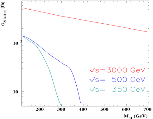
Figure 4.1: Inclusive Higgs production cross section as a function of the Higgs mass $M_{H}$ for three values of the $e^{+}e^{-}$ centre-of-mass energy $\sqrt{s}$

4.1.1 $H\to\mu^{+}\mu^{-}$

Measuring the muon Yukawa coupling by the determination of the $H^{0}\rightarrow\mu^{+}\mu^{-}$ branching fraction would complete the test of the scaling of the Higgs couplings to gauge bosons, quarks and leptons separately, ensuring that the observed Higgs boson is indeed responsible for the masses of all types of elementary particles. A data set of 3 ab^-1 at 3 TeV corresponds to 400 $H\rightarrow\mu\mu$ decays, for $M_{H}$ = 120 GeV, assuming Standard Model couplings. The main background from $WW\rightarrow\mu\nu\mu\nu$ can be reduced by cuts on the dimuon recoil mass and energy. The total background has been estimated including also the $ZZ\nu\bar{\nu}$, $WW\nu\bar{\nu}$ and the inclusive $\mu\mu\nu\bar{\nu}$ processes, evaluated without the Higgs contribution. The resulting dimuon invariant mass for all particle species is shown in Fig. 4.2. A signal significance of more than $5\sigma$ is obtained up to $M_{H}\simeq$ 155 GeV. The number of signal events is extracted from a fit to the dimuon invariant mass, where the signal is modelled by a Gaussian distribution peaked at the nominal Higgs mass and the background by a polynomial curve fitted on the peak side bands. The accuracies in the product of production cross section and $\mu\mu$ decay branching fraction, derived from the fitted number of signal events, are summarized in Table 4.1 for different values of $M_{H}$.

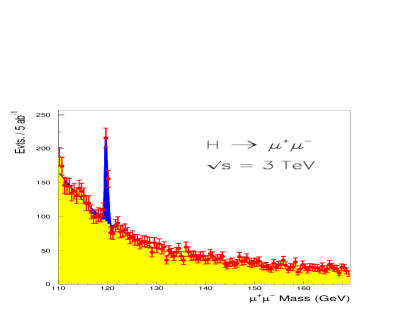
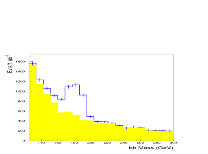
Figure 4.2: Reconstructed signals for $H^{0}\to\mu^{+}\mu^{-}$ (left) and $H^{0}\to b\bar{b}$ (right) for $M_{H}$ = 120 GeV and 200 GeV, respectively, at $\sqrt{s}$ = 3 TeV

Table 4.1: Statistical accuracy on the $g_{H\mu\mu}$ coupling expected with an integrated luminosity of 3 ab^-1 at $\sqrt{s}$ = 3 TeV, for different values of the Higgs boson mass, $M_{H}$

$M_{H}$	120 GeV	140 GeV	150 GeV
$\delta g_{H\mu\mu}/g_{H\mu\mu}$	0.042	0.065	0.110

These accuracies are comparable to those achievable with a muon collider operating at the Higgs mass peak [7], and more than a factor of 2 better than those expected at a very large hadron collider (VLHC) with a centre-of-mass energy of 200 TeV [8].

4.1.2 $H\to b\bar{b}$ for an Intermediate-Mass Higgs Boson

The scaling of the Higgs couplings to fermions also needs to be tested for Higgs bosons of intermediate mass. Beyond the $H\to WW$ threshold, the branching fractions $H\to f\bar{f}$ fall rapidly with increasing $M_{H}$ values. The process $e^{+}e^{-}\rightarrow\nu\bar{\nu}H\rightarrow b\bar{b}$ at $\sqrt{s}\geq$ 1 TeV still offers a favourable signal-to-background ratio for probing $g_{Hbb}$ for these intermediate-mass Higgs bosons. The $H^{0}\to b\bar{b}$ decay can be measured for masses up to about 240 GeV, with the accuracies summarized in Table 4.2.

Table 4.2: Signal significance and relative accuracy for the determination of the $b$ Yukawa coupling for different values of the $M_{H}$ mass at $\sqrt{s}$ = 3 TeV

$M_{H}$ (GeV)		$S/\sqrt{B}$	$\delta~{}g_{Hbb}~{}/~{}g_{Hbb}$
180		40.5	0.016
200		25.0	0.025
220		18.0	0.034

These accuracies are comparable to those expected for a light Higgs at a 300–500 GeV LC. They will ensure an accurate test of the Yukawa coupling to quarks for masses up to the limit set by the electroweak data for the Standard Model Higgs boson.

4.1.3 Triple Higgs Coupling and Reconstruction of the Higgs Potential

Another fundamental test of the Higgs sector with a light Higgs boson, which would benefit significantly from multi-TeV data, is the study of the Higgs self-couplings and the reconstruction of the Higgs potential. We recall that symmetry breaking in the Standard Model is completely encoded in the scalar Higgs potential. With the assumption of one Higgs doublet $\Phi$, the most general potential takes the form [9, 10]:

$$V_{{\cal{S}}{\cal{S}}{\cal{B}}}=\lambda\left\{\sum_{n=2}\frac{g^{2(n-2)}}{\Lambda^{2(n-2)}}\frac{a_{n}}{(n-1)^{2}}\left[\Phi^{\dagger}\Phi-\frac{v^{2}}{2}\right]^{n}\right\}\,,$$ (4.1)

in order that spontaneous symmetry breaking ensues with the correct value of the vacuum expectation value that gives the gauge bosons correct masses. The leading dimension-4 operator with $n$ = 2 above corresponds to the minimal Standard Model realization. In particular, this fixes the mass of the Higgs $M_{H}$ and its self-couplings in terms of a single parameter, $\lambda$. Higher-order operators may change the relationship between the Higgs mass and its self-couplings, as well as the couplings to the Goldstone bosons. Taking into account dimension-6 operators, and denoting the Goldstone bosons by $\phi_{3}$ and $\phi^{\pm}$ and the Higgs boson with $H$, Eq. (4.1) leads to:

$$V_{{\cal{S}}{\cal{S}}{\cal{B}}} = \frac{1}{2}M_{H}^{2}\left\{H^{2}+\frac{g}{M_{W}}H\,\left(\Phi^{+}\Phi^{-}+\frac{\Phi_{3}^{2}}{2}\right)+\,\frac{g}{2M_{W}}\,h_{3}H^{3}\,+\right.$$ (4.2)

$$\;\;\;\;\;\left.h_{4}\left(\frac{g}{4M_{W}}\right)^{2}H^{4}+h_{3}^{\prime}\left(\frac{g}{2M_{W}}\right)^{2}H^{2}\left(\Phi^{+}\Phi^{-}+\frac{\Phi_{3}^{2}}{2}\right)...\right\}$$

$$h_{3} \equiv g_{HHH}=1+a_{3}\frac{M_{W}^{2}}{\Lambda^{2}}=1+\delta h_{3}\,,\quad h_{4}\equiv g_{HHHH}=1+6\delta h_{3}\,,\quad h_{3}^{\prime}=1+3\delta h_{3}\;.$$

Probing the Higgs potential amounts to measuring the self-couplings of the Higgs, of which the most accessible is the trilinear coupling.

The triple-Higgs coupling $g_{HHH}$ can be accessed at a TeV-class LC in the double-Higgs production process $e^{+}e^{-}\to HHZ$ [11]. However, this measurement is made difficult by the tiny production cross section and by the dilution due to diagrams, leading to double Higgs production, that are not sensitive to the triple Higgs vertex. It has been concluded that a LC operating at $\sqrt{s}$ = 500 GeV can measure the $HHZ$ production cross section to about 15% accuracy if the Higgs boson mass is 120 GeV, corresponding to a fractional accuracy of 23% in $g_{HHH}$ [12].

This accuracy can be improved by performing the analysis at multi-TeV energies, as seen in Fig. 4.3,

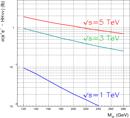
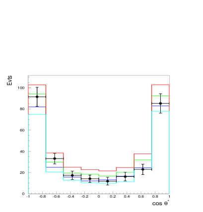
Figure 4.3: Double Higgs production at CLIC: cross section for the $e^{+}e^{-}\to HH\nu\bar{\nu}$ process as a function of the Higgs boson mass for different centre-of-mass energies (left) and the $|\cos\theta^{*}|$ distributions for different values of the triple Higgs coupling (right). A combined fit to the cross section and the decay angle distribution is used to extract the triple Higgs coupling.

using the process $e^{+}e^{-}\to HH\nu\bar{\nu}$ and introducing observables sensitive to the presence of the triple-Higgs vertex. The $H^{*}\to HH$ decay angle $\theta^{*}$ in the $H^{*}$ rest frame, which is sensitive to the scalar nature of the Higgs boson, has been adopted for the $HH\nu\bar{\nu}$ process. The resulting distribution in $|\cos\theta^{*}|$ is flat for the signal, while it is peaked forward for the other diagrams leading to the $HH\nu\bar{\nu}$ final state. Results are summarized in Table 4.3 [13]. No polarization has been included in this study. However, the double Higgs production for polarized beams is four times larger, indicating a further potential improvement of the accuracy by a factor of 2. Assuming that only some fraction of the time favorable polarized beams will be used, the precision is on the triple-Higgs coupling will be in the range of 0.07 to 0.09.

Table 4.3: Relative accuracy for the determination of the triple-Higgs coupling $g_{HHH}$ for different values of the $M_{H}$ mass at $\sqrt{s}$ = 3 TeV, assuming unpolarized beams

$M_{H}$ (GeV)		Counting	Fit
120		$\pm$ 0.131 (stat)	$\pm$ 0.093 (stat)
180		$\pm$ 0.191 (stat)	$\pm$ 0.115 (stat)

A qualitative study of the channel $e^{+}e^{-}\rightarrow H\nu\nu$ was further made at the generator level, taking into account both background and signal, for a wider range of Higgs masses (120 to 240 GeV) and several CMS energies (1.5 to 5 TeV). Figure 4.4 shows the cross section of the processes, the sensitivity of the cross section to the triple Higgs coupling, and and the expected precision with which the triple Higgs coupling can be determined. The calculations include the branching ratios into the relevant channels, and a reconstruction efficiency as determined for 3 TeV, using the fast simulation. The assumed integrated luminosity is 5 ab^-1.

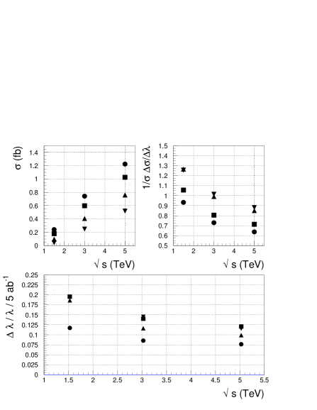
Figure 4.4: The cross section of the processes $e^{+}e^{-}\rightarrow H\nu\nu$, the sensitivity of the cross section to the triple Higgs coupling, and the expected precision with which the triple Higgs coupling, for the masses 120 GeV (circle), 140 GeV (box), 180 GeV (traingle), and 240 GeV (inverse triangle), for 5 ab^-1

The figure shows that for all Higgs masses concerned, a 3 TeV CLIC will give a measurement of the triple Higgs coupling with a precision of 10–15%. If the Higgs is relatively heavy one can gain in precision by operating CLIC at a higher (centre-of-mass system) (CMS) energy. Note that these numbers do not include beam polarization and do not use a topological selection, as was done for the more detailed study reported above. Hence one can gain another 30-50% in precision.

On the other hand, the quartic Higgs coupling remains elusive at CLIC, due to the smallness of the relevant triple-Higgs production cross sections. Even a 10-TeV collider would be able to produce only about five such events in one year (= 10⁷s) of operation at a luminosity of 10³⁵ cm^-2s^-1, while the dilution of the quartic coupling sensitivity is large owing to the effect of the background diagrams in $HHH\nu\bar{\nu}$, as seen in Table 4.4.

Table 4.4: Production cross sections for $e^{+}e^{-}\rightarrow HHH\nu\bar{\nu}$ at various centre-of-mass energies for different values of the quartic Higgs coupling

$\sqrt{s}$		$\frac{g_{HHHH}}{g_{HHHH}^{SM}}$ = 0.9	$\frac{g_{HHHH}}{g_{HHHH}^{SM}}$ = 1.0	$\frac{g_{HHHH}}{g_{HHHH}^{SM}}$ = 1.1
3 TeV		0.400	0.390	0.383
5 TeV		1.385	1.357	1.321
10 TeV		4.999	4.972	4.970

A further important advantage of multi-TeV $e^{+}e^{-}$ collisions is that heavier Higgses can also be scrutinized. Despite the much reduced cross section for heavier Higgs masses, any deviation in the Higgs self-couplings gets amplified as the Higgs mass gets higher, and can easily make up for the reduction in cross section that occurs for a Higgs with standard self-couplings. This is illustrated in Fig. 4.5 for $e^{+}e^{-}\;\rightarrow\nu\bar{\nu}HH$.

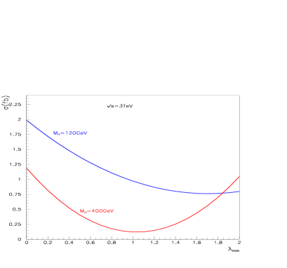
Figure 4.5: The $e^{+}e^{-}\;\rightarrow\nu\bar{\nu}HH$ signal and background, together with the total cross section, as functions of the Higgs mass for $\sqrt{s}$ = 2 TeV. The second panel shows how the cross section varies as a function of $g_{HHH}$ for $M_{H}$ = 120, 400 GeV at $\sqrt{s}$ = 3 TeV.

The signal is identified by the contribution of the diagram containing the $g_{HHH}$ coupling normalized to its Standard Model value, $g_{HHH}$ = 1, and the remaining contributions are identified as background. The signal increases as a function of the Higgs mass up to about $M_{H}$ = 350 GeV, before dropping. For higher centre-of-mass energies, this turnover occurs for even higher masses, and the background decreases at the same time. As the Higgs mass increases, a subtle cancellation between these two contributions takes place. This leads to a precipitous drop in the total cross section for a Standard Model Higgs boson. This type of cancellation is reminiscent of what occurs in $e^{+}e^{-}\rightarrow W^{+}W^{-}\;$between the neutrino exchange and the triple vector gauge coupling diagrams. If the $g_{HHH}$ strength deviates slightly from unity, this cancellation may not be effective, and would increase the cross section, as shown in the second panel of Fig. 4.5. A deviation in $g_{HHH}$ has a more drastic effect for $M_{H}$ = 400 GeV than for $M_{H}$ = 120 GeV. For example, for $g_{HHH}$ = 2 the cross section is larger for $M_{H}$ = 400 GeV than for $M_{H}$ = 120 GeV.

This behaviour can easily be explained, if we recall that in this case double Higgs production is due to longitudinal $W$ bosons that can be identified at these high energies with the charged Goldstone modes. The amplitude for $W_{L}W_{L}\rightarrow HH$ may be approximated as

$$\tilde{\cal M}_{W_{L}W_{L}\rightarrow HH}\rightarrow\frac{g^{2}}{4}r(3h_{3}-2)+\dots,\quad r=M_{H}^{2}/M_{W}^{2}\,.$$ (4.3)

Not only does this reveal the enhanced coupling factor $r=M_{H}^{2}/M_{W}^{2}$, but it also shows that, if $h_{3}$ deviates from its standard value, the cancellation between signal and background is disrupted. Even in the present absence of a full simulation for the extraction of the Higgs self-couplings for high Higgs masses, we can attempt to derive some limit for $M_{H}$ = 400 GeV, since a naive 3$\sigma$ limit for $M_{H}$ = 120 GeV reproduces quite closely the result of a more detailed analysis. For $M_{H}$ = 400 GeV, both the produced $H$ bosons will usually decay into a $WW$ pair. We take $\int{\cal L}$ = 5 ab^-1 and assume 50% efficiency for the reconstruction of the $WWWW,WWZZ$ and $ZZZZ$ final states. A 3$\sigma$ accuracy on the cross section leads to the constraint 0.88 $<g_{HHH}<$ 1.18, i.e., a precision of about 15% on the trilinear self-coupling of the Higgs boson.

4.1.4 Heavy Higgs Boson

The precision electroweak data indicate that the Higgs boson is probably lighter than about 212 GeV [14]. However, this limit can be evaded if new physics cancels the effect of the heavy Higgs boson mass. In these scenarios, it is interesting to search for a heavier boson through the $ZZ$ fusion process $e^{+}e^{-}\to H^{0}e^{+}e^{-}\to Xe^{+}e^{-}$ at high energies. Like the associated $HZ$ production in the Higgs-strahlung process at lower energies, this channel allows a model-independent Higgs search, through the tagging of the two forward electrons and the reconstruction of the mass recoiling against them [15]. This analysis needs to identify electrons and measure their energies and directions down to $\simeq$ 100 mrad, as seen in the left panel of Fig. 4.6. This is close to the bulk of the $\gamma\gamma\to{\mbox{\rm hadrons}}$ and pair backgrounds, creating a challenge for forward tracking and for the calorimetric response of the detector. Preliminary results show that a clean Higgs signal can be extracted at $\sqrt{s}$ = 3 TeV for $M_{H}\leq$ 900 GeV, as seen in the right panel of Fig. 4.6.

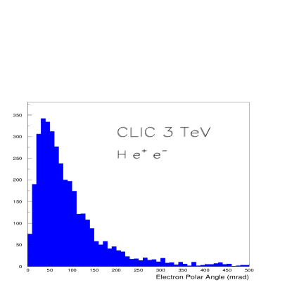
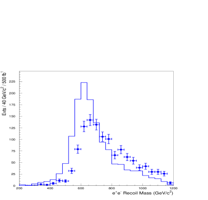
Figure 4.6: Left panel: The distribution of electron polar angles in $e^{+}e^{-}\to H^{0}e^{+}e^{-}$ events at CLIC with $E_{c.m.}$ = 3 TeV. Right panel: The distribution of recoil masses $M_{X}$ in $e^{+}e^{-}\to(H^{0}\to X)e^{+}e^{-}$ events at CLIC with $E_{c.m.}$ = 3 TeV.

4.2 Testing New Physics in the Higgs Sector

The accurate measurement of Higgs couplings achievable at the LC may reveal discrepancies with the SM predictions. These might provide us with a first signal that nature realizes the Higgs mechanism through a scalar sector, which is more complex than the minimal Higgs doublet of the SM. A minimal extension of the Higgs sector contains two complex scalar doublets, in which case the Higgs sector has five physical Higgs bosons: two that are CP-even and neutral ($h^{0}$ and $H^{0}$), one CP-odd and neutral ($A^{0}$) and two that are charged ($H^{\pm}$). In addition to the Higgs masses, there are two more parameters: the ratio ${\rm tan}\beta$ of the vacuum expectation values of the two fields and a mixing angle $\alpha$. In the minimal supersymmetric extension of the SM (MSSM) discussed here, only two of these parameters are independent.

4.2.1 Heavy MSSM Higgs Bosons

If the heavier Higgs bosons $H^{0},A^{0}$ and $H^{\pm}$ of a non-minimal Higgs sector are not too heavy, they will be pair-produced directly at a LC. At tree level, the production cross sections for $e^{+}e^{-}\rightarrow H^{+}H^{-}$ and $e^{+}e^{-}\rightarrow H^{0}A^{0}$ are independent of ${\rm tan}\beta$. In calculating the effective production cross section, initial-state radiation (ISR) and the beam–beam effects for the CLIC.01 parameters have been taken into account. As a result, for low values of $M_{H^{\pm}}$ the effective cross section is enhanced with respect to the tree-level cross section, while close to the kinematical threshold only a smaller fraction of the energy spectrum is available and the effective cross section is reduced, as seen in Fig. 4.7.

Figure 4.7: Heavy Higgs production at CLIC: the $e^{+}e^{-}\rightarrow H^{+}H^{-}$ (left) and $e^{+}e^{-}\rightarrow H^{0}A^{0}$ (right) production cross sections for $\sqrt{s}$ = 3 TeV, as functions of the Higgs mass

The sizeable production cross sections for the $H^{+}H^{-}$ and $H^{0}A^{0}$ pair production processes provide sensitivity at CLIC for masses up to about 1 TeV and beyond, for all values of ${\rm tan}\beta$, thus extending the LHC reach. For large values of $M_{A}$, the main processes of interest are $e^{+}e^{-}\rightarrow H^{+}H^{-}\rightarrow t\bar{b}\bar{t}b$ and $e^{+}e^{-}\rightarrow H^{0}A^{0}\rightarrow b\bar{b}b\bar{b}$ or $t\bar{t}t\bar{t}$. These result in highly distinctive, yet challenging, multijet final states with multiple $b$-quark jets, which must be identified and reconstructed efficiently. We now discuss each of these processes in turn.

4.2.1.1 $e^{+}e^{-}\rightarrow H^{+}H^{-}$

A detailed analysis has been performed for the reconstruction of $e^{+}e^{-}\rightarrow H^{+}H^{-}\rightarrow t\bar{b}\bar{t}b$ with $M_{H}$ = 880 GeV, corresponding to the constrained minimal supersymmetric standard model (CMSSM) benchmark point J of Ref. [16]. A sample Higgs analysis is illustrated in Fig. 4.8, whose left panel shows a simulation of a ‘typical’ $e^{+}e^{-}\rightarrow H^{+}H^{-}$ event. Event reconstruction is based on the identification of the $WbbWbb$ final state, and applies a mass-constrained fit to improve the mass resolution and reject multifermion and other combinatorial backgrounds [17], as seen in the right panel of Fig. 4.8. Events with no jet combination compatible with the $W$ or $t$ masses within the observed resolution have been discarded. The fit uses energy and momentum conservation, the $W$ and $t$ mass constraints, and imposes equal masses for the $H^{\pm}$ bosons. The cross section for the irreducible SM $e^{+}e^{-}\rightarrow t\bar{b}\bar{t}b$ background has been estimated to be 1.5 fb at $\sqrt{s}$ = 3 TeV.

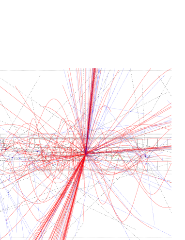
Figure 4.8: Charged-Higgs analysis. Left: Display of a $e^{+}e^{-}\rightarrow H^{+}H^{-}\rightarrow t\bar{b}\bar{t}b$ event at $\sqrt{s}$ = 3 TeV. The accelerator-induced backgrounds are not overlaid. Right: $H^{\pm}$ mass signal reconstructed before (continuous line) and after (dashed line) applying a global mass-constrained fit.

The superposition of accelerator-induced $\gamma\gamma\rightarrow{\mathrm{hadrons}}$ events has also been included. Here special care has been taken to make the result robust in the presence of all high-energy beam–beam effects. The additional hadrons generated by these $\gamma\gamma$ collisions, mostly in the forward regions, may either be merged into the jets coming from the $H^{\pm}$ decay or result in extra jets being reconstructed. In order to minimize the impact on the event reconstruction, only the four leading non-$b$ jets have been considered, together with the $b$-tagged jets. Besause of the significant loss of energy of the colliding $e^{+}$ and $e^{-}$, energy and momentum conservation constraints cannot be applied on the reconstructed system for the nominal $\sqrt{s}$. Instead, the kinematical fit allows for an extra particle to be radiated, but imposes its transverse momentum to be zero. This kinematical fit improves the Higgs mass resolution by a factor of nearly 2, as seen in Fig. 4.8.

The signal event rate has been estimated including the $\gamma\gamma$ background, assuming that the detector integrates over 15 bunch crossings. The fitted signal width is 45 GeV after the mass-constrained fit and there are 149 $e^{+}e^{-}\rightarrow H^{+}H^{-}\rightarrow(t\bar{b})(\bar{t}b)$ signal events with a reconstructed mass in the signal window, corresponding to an efficiency of 0.05. The $tbtb$ SM background processes contribute 43 events for 3 ab^-1. By scaling these results, the estimated maximum mass reach for a 5$\sigma$ discovery with 3 ab^-1 at 3 TeV is 1.25 TeV if the $tb$ mode saturates the $H$ decay width, or 1.20 TeV if it accounts for only 0.85% of the decays.

By reconstructing either both the $H^{\pm}$ or only one, the analysis can be optimized in terms of efficiency and resolution for either mass measurement or an unbiased study of $H^{\pm}$ decays, respectively. Fractional accuracies of 0.5–1.0% on the heavy boson mass for 600 $<M_{H}<$ 900 GeV and of 5–7% on the product of production cross section and $tb$ decay branching fraction are expected with ${\cal{L}}$ = 3 ab^-1 at $\sqrt{s}$ = 3 TeV. The results do not depend critically on the underlying hadronic background.

4.2.1.2 $e^{+}e^{-}\to H^{0}A^{0}$

A similar study has been performed for the reconstruction of the $e^{+}e^{-}\to H^{0}A^{0}\to b\bar{b}b\bar{b}$ process, as illustrated in Fig. 4.9. The reconstruction has been based on the identification of two pairs of $b$-tagged jets with close invariant masses. Again, masses have been chosen to correspond to the CMSSM benchmark point J, which has $M_{A}$ = 876 GeV. The reconstruction is based on the identification of two pairs of $b$-tagged jets with equal dijet masses. Similarly to the study of charged Higgs bosons, a kinematical fit has been applied, imposing energy and momentum conservation and equal masses. Energy loss due to initial-state radiation and beamstrahlung has also been accounted for, as described above. Owing to the simpler final state considered for this analysis, the efficiency for $e^{+}e^{-}\to H^{0}A^{0}\to\bar{b}b\bar{b}b$ is about seven times larger than that obtained for $e^{+}e^{-}\to H^{+}H^{-}\to t\bar{b}\bar{t}b$. After reduction of the SM $e^{+}e^{-}\rightarrow bbbb$ background, the discovery potential for $e^{+}e^{-}\to A^{0}H^{0}$ in the $bbbb$ final states extends to $M_{A}\leq$ 1.3 TeV, for an integrated luminosity of 3 ab^-1. The reconstruction yields relative accuracies of 0.004 and 0.062 for the measurement of the $A^{0}$ mass and of the signal event rate, respectively, for the CMSSM benchmark point J which has BR($H$, $A\to b\bar{b}$) = 0.87.

For low values of ${\rm tan}\beta$, the main decay channel is $A^{0}$, $H^{0}\to\bar{t}t$. The analysis in this channel is based on the reconstruction of the hadronic decays of the four $W$ bosons and the identification of the four $b$ jets. Because of the complex final state, the signal efficiency reaches only 2% in this channel. After reduction of the SM $e^{+}e^{-}\rightarrow t\bar{t}\bar{t}t$ background, the discovery potential is up to about 1.1 TeV, for 3 ab^-1.

The relative accuracies achievable on the mass and production cross sections are $\delta M_{A}/M_{A}$ = 0.012 and $\delta\sigma_{HA}/\sigma_{HA}$ = 0.075, respectively, assuming $m_{A}$ = 576 GeV and the $\bar{t}t$ channel saturating the decay width. The CLIC mass reach for observing the $A^{0}$ and $H^{0}$ bosons as function of ${\rm tan}\beta$ is shown in Fig. 4.9.

Figure 4.9: Neutral Higgs analysis. Left: The signal reconstructed in the $e^{+}e^{-}\to H^{0}A^{0}\to b\bar{b}\bar{b}b$ for the CMSSM point J. Right: The $H^{0}A^{0}$ discovery reach with 3 ab^-1 of CLIC data at 3 TeV as a function of ${\rm tan}\beta$ obtained by summing the $b\bar{b}\bar{b}b$ and $t\bar{t}\bar{t}t$ channels.

4.2.1.3 $\gamma\gamma\rightarrow H,A$

Photons generated by Compton back-scattering of laser light off the incoming $e^{-}$ beams can reach c.m. energies of 70–80% of the primary collider energies and high degrees of polarization [18]. Higgs bosons can be produced as s-channel resonances and thus the full (photon) beam energy can be used to produce the heavy particles. In this way, $\gamma\gamma$ colliders can extend the Higgs discovery to higher mass regions than $e^{+}e^{-}$ colliders with the same centre-of-mass energies. With integrated annual luminosities of 100–200 fb^-1, sufficiently high signal rates are guaranteed so that photon colliders provide a useful instrument for the search of Higgs bosons in regions of the parameter space not accessible elsewhere [19].

The decay channel $H,A\to b\bar{b}$ is particularly promising for the $H$ and $A$ discovery. Figure 4.10 shows the branching ratios of $H,A$ [20, 21] for ${\rm tan}\beta$ = 7 and $M_{H,A}>$ 200 GeV, a parameter region not covered by LHC discovery modes. The higgsino and gaugino MSSM parameters have been set to $|\mu|=M_{2}$ = 200 GeV, with a universal gaugino mass at the GUT scale. Squarks and sleptons are assumed to be so heavy that they do not affect the results significantly. Results are shown for both signs of the $\mu$ parameter. Owing to the enhancement of the MSSM Higgs boson couplings to $b\bar{b}$ at large ${\rm tan}\beta$, the $b\bar{b}$ decay is sizeable and dominates for moderate masses.

Figure 4.10: Branching ratios of the heavy Higgs bosons $H,A$ as a function of the corresponding Higgs mass: $\tilde{\chi}^{0}\tilde{\chi}^{0}$ ($\tilde{\chi}^{+}\tilde{\chi}^{-}$) represents the sum of all neutralinos (charginos) except the lightest neutralino pair

Figure 4.11 shows the result for $\gamma\gamma\to b{\bar{b}}$ and polarized $e^{-}$ and laser photon beams for ${\rm tan}\beta$ = 7 and $M_{H,A}>$ 200 GeV. The NLO QCD corrections to the signal [20, 22], background [23] and interference term [19] have been included. Since the signals are generated for equal photon helicities, the initial beam polarizations have been chosen such that this configuration is enhanced. Assuming that evidence for a Higgs boson has been found in a preliminary rough scan of the $\gamma\gamma$ energy, the maximum of the $\gamma\gamma$ luminosity spectrum, which is at 70–80% of the $e^{\pm}e^{-}$ c.m. energy for equal photon helicities [18, 24], has been tuned to the mass $M_{A}$. The analysis can be optimized by applying final-state cuts. A cut in the production angle of the bottom quarks, $|\cos\theta|<0.5$, strongly reduces the background, whereas the signal is affected only moderately. By collecting $b\bar{b}$ final states with an expected resolution $M_{A}\pm$ 3 GeV [25], the sensitivity to the resonance signal above the background is strongly increased. Furthermore, in order to suppress gluon radiation, which increases the background at NLO in the same-helicity configuration, slim two-jet configurations have been selected in the final state as defined within the Sterman–Weinberg criterion; events with radiated gluon energies above 10% of the $\gamma\gamma$ invariant energy and opening angles between the three partons exceeding 20^∘ have been rejected. Higher-order corrections beyond NLO, which become important in the two-jet final states, have been taken into account by (non-)Sudakov form factors [26].

As can be inferred from Fig. 4.11, the background is strongly suppressed (even if the experimental resolution is less favourable than assumed) and the significance of the heavy Higgs boson signals is sufficient for the discovery of the Higgs particles up to about 0.8–1 TeV, if about 10–20 events are needed for the discovery. In order to reach higher masses more luminosity needs to be accumulated. The discovery/measurement reach increases in this channel for higher ${\rm tan}\beta$ values, as shown in Fig. 4.11(right).

Figure 4.11: Left: Sum of the signal, background and interference cross sections (full, dashed lines) for the resonant $H,A$ production in $\gamma\gamma$ fusion as a function of $M_{A}$ with final decays into $b\bar{b}$, and the corresponding background cross section. The SUSY parameters are chosen as ${\rm tan}\beta$ = 7, $M_{2}=\pm\mu$ = 200 GeV. For comparison the cross section in the case of vanishing supersymmetric-particle contributions is also shown. Right: The same as on the left, but for ${\rm tan}\beta$ = 15.

The production of Higgs bosons $h,H,A$ in $\gamma\gamma$ collisions may serve a second purpose beyond discovery. The formation of Higgs bosons in $\tau^{+}\tau^{-}$ collisions, with the $\tau$’s generated in the splitting of the two photons, $\gamma+\gamma\to(\tau^{+}\tau^{-})(\tau^{+}\tau^{-})\to(\tau^{+}\tau^{-})+h/H/A$, is very sensitive to ${\rm tan}\beta$ for high values, cf. Ref. [27]. The production cross section rises quadratically with ${\rm tan}\beta$ in this regime, $\sigma_{\gamma\gamma}\approx{\rm tan}^{2}\beta$, so that the mixing parameter can be measured very well by this method. With expected accuracies $\Delta{\rm tan}\beta/{\rm tan}\beta$ at a level of 5 to 10%, sufficiently below the kinematical limit [specifically, $\Delta{\rm tan}\beta/{\rm tan}\beta\simeq$ 5.7% [$H+A$] for $M_{H,A}$ = 500 GeV, $\sqrt{s_{\gamma\gamma}}$ = 2 TeV and $L$ = 500 fb^-1, this $\gamma\gamma$ method of Higgs analyses can improve significantly on complementary measurements in channels at the LHC and in the $e^{+}e^{-}$ mode of a linear collider.

4.2.2 CP Violation in the Supersymmetric Higgs Sector

Several of the soft supersymmetry-breaking parameters of the MSSM can have a complex phase, inducing new sources of CP violation in addition to the phase in the Cabbibo–Kobayashi–Maskawa matrix of the SM, even if minimal flavour violation is assumed, as here. The phenomenology of such an MSSM with complex parameters (CMSSM) can be substantially different from the case in which all the soft supersymmetry-breaking parameters are assumed to be real (see, for example, Ref. [28] for an analysis concerning LEP constraints on the Higgs sector in the CMSSM). The possibly complex parameters are the trilinear Higgs–sfermion couplings, $A_{q},q~{}=~{}t,b,\tau,\ldots$, the Higgs mixing parameter $\mu$, and the soft supersymmetry-breaking gaugino mass parameters $M_{1}$, $M_{2}$, $M_{3}$.

The situation becomes simpler in the constrained version of the MSSM with universal soft supersymmetry-breaking scalar masses $m_{0}$, gaugino masses $m_{1/2}$, and trilinear couplings $A_{0}$ (the CMSSM) input at some high scale. In this case there are just two new sources of CP violation. In a suitable convention, these can be chosen as the phases of the complex parameters $m_{1/2}$ and $A_{0}$ relative to that of the Higgs mixing parameter $\mu$. The values of these phases are constrained by the upper limits on the electric dipole moments (EDMs) of the electron, neutron [29, 30] and mercury atom [31] and other measurements, but large CP-violating phases in $m_{1/2}$ and in the third-generation trilinear couplings $A_{0}$ cannot yet be excluded. The ongoing probes of CP violation at $B$ factories can test the consistency of this and other non-minimal CP-violating supersymmetric scenarios [32, 33].

At the tree level, the Higgs boson sector of the CMSSM is CP-invariant. However, taking radiative corrections into account, all three neutral Higgs bosons, $h$, $H$, and $A$ can mix with each other [34, 35]. Thus the charged Higgs boson mass $M_{H^{\pm}}$ is the best choice as input parameter, contrary to the case of the real MSSM, where $M_{A}$ is usually chosen as input. In the approximation of vanishing external momentum the mixing can be written as

$$\left(\begin{array}[]{c}H_{1}\\ H_{2}\\ H_{3}\end{array}\right)\;=\;\mathbf{O}\left(\begin{array}[]{c}h\\ H\\ A\end{array}\right)~{},\qquad\mathbf{O}=\left(\begin{array}[]{ccc}O_{11}&O_{12}&O_{13}\\ O_{21}&O_{22}&O_{23}\\ O_{31}&O_{32}&O_{33}\end{array}\right)\,,$$ (4.4)

with

$$m_{H_{1}}\leq m_{H_{2}}\leq m_{H_{3}}\,.$$ (4.5)

This mixing is induced by sizeable off-diagonal scalar–pseudoscalar contributions ${\cal M}^{2}_{SP}$ [35, 36, 37, 38] to the general 3 $\times$ 3 Higgs-boson mass matrix. Each of the individual CP-violating off-diagonal scalar–pseudoscalar mixing entries ${\cal M}^{2}_{\rm SP}$ in the neutral MSSM mass-squared matrix contains terms scaling qualitatively as

$${\cal M}^{2}_{\rm SP}\ \sim\ \frac{m^{4}_{t}}{v^{2}}\,\frac{{\rm Im}\,(\mu A_{t})}{32\pi^{2}\,M^{2}_{\rm SUSY}}\ \bigg{(}1,\ \frac{|A_{t}|^{2}}{M^{2}_{\rm SUSY}}\,,\ \frac{|\mu|^{2}}{\tan\beta\,M^{2}_{\rm SUSY}}\,,\ \frac{2{\rm Re}\,(\mu A_{t})}{M^{2}_{\rm SUSY}}\,\bigg{)}\,,$$ (4.6)

at the one-loop level, which could be of order $M^{2}_{Z}$. The gluino phase contributes at two-loop order. In Eq. (4.6), $M^{2}_{\rm SUSY}$ denotes a common soft supersymmetry-breaking scale defined by the arithmetic average of the squared stop masses.

Furthermore, the effective couplings of Higgs bosons to bottom and top squarks [39] can be affected by the additional CP violation [35, 38]. These effective couplings are induced by loops involving gluinos and higgsinos, as well as top and bottom squarks. Although these effects enter the charged and neutral Higgs-boson masses and couplings formally at the two-loop level, they can still modify the numerical predictions or masses and couplings in a significant way, and therefore have to be included in the analysis.

Two of the main production mechanisms for producing neutral Higgs bosons in $e^{+}e^{-}$ collisions are the Higgs-strahlung process and the pair-production reaction:

$$e^{+}e^{-}\to ZH_{i} \qquad{\rm with}\qquad i=1,2,3$$ (4.7)

$$e^{+}e^{-}\to H_{i}H_{j} \qquad{\rm with}\qquad i\neq j,\;i,j=1,2,3~{}.$$ (4.8)

The effective $H_{i}ZZ$ and $H_{i}H_{j}Z$ couplings are given by

$${\cal L}_{\rm int} = \frac{g_{w}}{2\cos\theta_{w}}\,\bigg{[}\,M_{Z}\,\sum\limits_{i=1}^{3}\,g_{H_{i}ZZ}\,H_{i}Z_{\mu}Z^{\mu}\>+\>\sum\limits_{j>i=1}^{3}\,g_{H_{i}H_{j}Z}\,(H_{i}\,\!\!\stackrel{{\scriptstyle\leftrightarrow}}{{\vspace{2pt}\partial}}_{\!\mu}H_{j})\,Z^{\mu}\,\bigg{]}\,,$$ (4.9)

where $\cos\theta_{w}\equiv M_{W}/M_{Z}$, $\stackrel{{\scriptstyle\leftrightarrow}}{{\vspace{2pt}\partial}}_{\!\mu}\ \equiv\ \stackrel{{\scriptstyle\rightarrow}}{{\vspace{2pt}\partial}}_{\!\mu}-\stackrel{{\scriptstyle\leftarrow}}{{\vspace{2pt}\partial}}_{\!\mu}$, and

$$g_{H_{i}ZZ} = \cos\beta\,O_{1i}\>+\>\sin\beta\,O_{2i}\,,$$

$$g_{H_{i}H_{j}Z} = O_{3i}\,\Big{(}\cos\beta\,O_{2j}\,-\,\sin\beta\,O_{1j}\Big{)}\ -\ O_{3j}\,\Big{(}\cos\beta\,O_{2i}\,-\,\sin\beta\,O_{1i}\Big{)}\,.$$ (4.10)

From the above coupling structure it follows that

• the effective couplings $H_{i}ZZ$ and $H_{i}H_{j}Z$ are related to each other through

  $$g_{H_{k}ZZ}\ =\ \varepsilon_{ijk}\,g_{H_{i}H_{j}Z}\,,\quad{\rm and}$$ (4.11)

• unitarity leads to the coupling sum rule [40]

  $$\sum\limits_{i=1}^{3}\,g_{H_{i}ZZ}^{2}\ =\ 1\,,$$ (4.12)

  which reduces the number of independent $H_{i}ZZ$ and $H_{i}H_{j}Z$ couplings.

It is obvious from Eq. (4.6) that CP-violating effects on the neutral Higgs-boson mass matrix become significant when the product ${\rm Im}\,(\mu A_{t})/M^{2}_{\rm SUSY}$ is large. Motivated by this observation, the following CP-violating benchmark scenario (CPX) is defined as [41]:

$$\widetilde{M}_{Q}\! = \!\widetilde{M}_{t}\ =\ \widetilde{M}_{b}\ =\ M_{\rm SUSY}\,,\qquad\qquad\mu\ =\ 4M_{\rm SUSY}\,,$$

$$|A_{t}|\! = \!|A_{b}|\ =\ 2M_{\rm SUSY}\,,\qquad\qquad{\rm arg}(A_{t})\ =\ 90^{\circ}\,,$$

$$|m_{\tilde{g}}|\! = \!1~{}{\rm TeV}\,,\qquad\qquad\hskip 42.67912pt{\rm arg}(m_{\tilde{g}})\ =\ 90^{\circ}\,,$$ (4.13)

where we follow the notation of Ref. [38]. Without loss of generality, the $\mu$ parameter is considered to be real. We note that the CP-odd phases ${\rm arg}(A_{t})$ and ${\rm arg}(m_{\tilde{g}})$ are chosen to take their maximal CP-violating values. In the following, we also discuss variants of the CPX scenario with other values of ${\rm arg}(A_{t})$ and ${\rm arg}(m_{\tilde{g}})$, keeping the other quantities fixed at the values in Eq. (4.2.2).

In Fig. 4.12, we display the masses of the two heaviest neutral Higgs bosons, $H_{2}$ and $H_{3}$, as functions of ${\rm arg}\,(A_{t})$, in the CPX scenario with ${\rm tan}\beta$ = 5, $M_{\rm SUSY}$ = 1 TeV. Going from the upper to the lower panel in Fig. 4.12, we vary the charged Higgs-boson pole mass: $M_{H^{\pm}}$ = 200, 400, 600 GeV. Numerical results pertaining to the effective-potential masses are indicated by solid lines, while the results of pole masses are given by the dashed lines.

Figure 4.12: Numerical estimates of the two heaviest $H_{2}$- and $H_{3}$-boson masses versus ${\rm arg}\,(A_{t})$ for different charged Higgs-boson pole masses in a CPX scenario with ${\rm arg}(m_{\tilde{g}})$ = 90^∘ and $M_{\rm SUSY}$ = 1 TeV. Effective-potential masses are indicated by solid lines and pole masses by dashed ones.

We see that the mass difference between the two heavier neutral Higgs bosons $H_{2}$ and $H_{3}$ may be very different from its value when ${\rm arg}\,(A_{t})~{}=~{}0$, because of repulsive CP-violating mixing between the two states. Although in general every possible mass difference for CP-violating parameters can also be reached in the real MSSM [42], the measurement of $m_{H_{3}}-m_{H_{2}}$ can give valuable information about the complex phases in the CMSSM Higgs sector. Measuring these mass differences accurately will require an $e^{+}e^{-}$ linear collider, which can only be CLIC if $M_{H^{\pm}}$ is large. As shown in the previous section, it should be possible to measure the $H^{\pm}$ and $H_{2,3}$ masses with an accuracy $\sim$ 1% at CLIC, smaller than the possible mass shifts shown in Fig. 4.12.

If the mass of the charged Higgs boson is large, $M_{H^{\pm}}\gg M_{Z}$, the lightest MSSM Higgs boson becomes an almost pure CP-even state, whilst the other two neutral Higgs bosons mix through a single mixing angle $\theta_{23}$ between the CP eigenstates $H$ and $A$. If the mixing is substantial, which can happen in certain parts of the CMSSM parameter space [42], determining the value of $\theta_{23}$ will be one of the most important measurements in the Higgs sector. Since $\theta_{23}$ can be strongly influenced by ${\rm arg}\,(A_{t})$ via the loop-corrected Higgs boson self-energies and the loop-induced Higgs boson mixing, one can expect a non-negligible numerical correlation between the two parameters.

In the limit when $M_{H^{\pm}}\gg M_{Z}$, the only mode for producing the neutral heavy Higgs bosons at CLIC is the associated production mechanism $e^{+}e^{-}\to Z^{*}\to H_{2}H_{3}$. Determining the angle $\theta_{23}$ can in principle be done in two different ways. In the first approach, the decay products of the $H_{2}$ and $H_{3}$ would have to be analysed. If the $H_{2,3}\to\tau^{+}\tau^{-}$ channels have sufficiently large branching ratios, the $\tau$ polarizations might be used to get a handle on $\theta_{23}$ [43]. However, for $m_{H_{2,3}}\;\raisebox{-3.87495pt}{$\textstyle\stackrel{{\scriptstyle\textstyle>}}{{\sim}}$}\;2m_{t}$ the $\tau^{+}\tau^{-}$ decay branching ratio becomes strongly suppressed, and other methods to determine $\theta_{23}$ become more interesting.

We have analysed the correlation of the branching ratios of $H_{2}$ and $H_{3}$, the angle $\theta_{23}$ and the phase ${\rm arg}\,(A_{t})$ for $M_{H^{\pm}}$ = 300, 400 GeV. Assuming heavy charginos, the relevant decay channels for the heavy Higgs bosons are in this case

$$H_{2,3}\;\to\;\bar{t}t,\;\bar{b}b,\;\tau^{+}\tau^{-},\;\bar{\tilde{t}}_{1}{\tilde{t}_{1}},\;H_{1}H_{1}\,.$$ (4.14)

Any of these channels is of course absent if it is kinematically forbidden. If the $\bar{\tilde{t}}_{1}{\tilde{t}_{1}}$ channel is allowed, it usually dominates the other decays, and hardly any variation of the branching ratios with ${\rm arg}\,(A_{t})$ can be observed. Therefore we focus on the more favourable scenarios in which ${\tilde{t}_{1}}$ is too heavy to be produced in Higgs decays.

As representative sample parameters, we choose ${\rm tan}\beta$ = 5, $M_{\rm SUSY}$ = 500 GeV, $|A_{t}|~{}=~{}A_{b}~{}=~{}A_{\tau}$ = 1200 GeV, $\mu$ = 800 GeV, $M_{2}$ = 400 GeV and $m_{\tilde{g}}$ = 500 GeV. We vary ${\rm arg}\,(A_{t})$ in the interval $[0,\pi/2]$ radians, and note that a measurement of ${\rm arg}\,(A_{t})$ thus corresponds directly to a determination of $\theta_{23}$. Our evaluations have been performed with FeynHiggs2.0 [44, 45], taking into account corrections up to the two-loop level in the Higgs boson masses, mixing and decays. The results for $M_{H^{\pm}}$ = 300, 400 GeV are shown in the left and right plots of Fig. 4.13, respectively. Since it will be nearly impossible to distinguish the decay of the $H_{2}$ from that of the $H_{3}$, we have averaged over the two branching ratios, i.e. what is shown in Fig. 4.13 is $[{\rm BR}(H_{2}\to X)+{\rm BR}(H_{3}\to X)]/2$. For $M_{H^{\pm}}$ = 300 GeV, the channel $H_{2,3}\to\bar{t}t$ is absent, whilst for $M_{H^{\pm}}$ = 400 GeV it is dominant. Thus these two different choices of $M_{H^{\pm}}$ represent two distinct cases for the branching-ratio analysis.

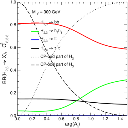
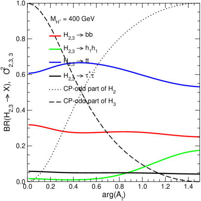
Figure 4.13: The principal branching ratios (see text) and the CP-odd parts $\sim\cos^{2}\theta_{23},\sin^{2}\theta_{23}$ of $H_{2}$ and $H_{3}$ are shown as functions of ${\rm arg}\,(A_{t})$. In the left (right) plot the charged Higgs boson mass is set to $M_{H^{\pm}}$ = 300 (400) GeV. The other parameters are specified in the text.

Together with the branching ratios, we also display the CP-odd parts of $H_{2}$, scaling like $\cos^{2}\theta_{23}$, and of $H_{3}$, scaling like $\sin^{2}\theta_{23}$. The numerical correlations between the branching ratios, ${\rm arg}\,(A_{t})$ and $\{\cos,\sin\}^{2}\theta_{23}$ can be read off from the plots. Therefore, a precise measurement of ${\rm arg}\,(A_{t})$ via the branching ratios would allow one to retrieve information about $\theta_{23}$. However, one should keep in mind that we have varied only one parameter and kept the others fixed. This would correspond to perfect experimental knowledge of the other parameters, which is of course an unrealistic assumption. However, the potential for determining $\theta_{23}$ and ${\rm arg}\,(A_{t})$ in this way is nevertheless demonstrated in this exploratory study.

Furthermore, the precision with which ${\rm arg}\,(A_{t})$ and $\theta_{23}$ can be determined depends strongly on the achievable precision of the branching-ratio measurement. The cross section at CLIC for the $e^{+}e^{-}\to Z^{*}\to H_{2}H_{3}$ production process is slightly larger than 1 fb [46], and is largely independent of the value of $M_{H^{\pm}}$, which results in about 1000 events for each collected 1 ab^-1. Unfortunately, no evaluation of the precision with which the branching ratios of the heavy neutral Higgs bosons could be measured at CLIC is yet available.

Finally, another possible observable in the MSSM with complex parameters is a difference in the decay rates of $H^{+}$ and $H^{-}$ [47]. For the $tb$ final state, the rate asymmetry

$$\delta^{\rm CP}\equiv\frac{\Gamma(H^{+}\to b\bar{t})-\Gamma(H^{-}\to t\bar{b})}{\Gamma(H^{+}\to b\bar{t})+\Gamma(H^{-}\to t\bar{b})}$$ (4.15)

can be induced by the one-loop diagrams shown in Fig. 4.14 [47]. For the numerical analysis of this possibility, we use

$$M_{2}=200~{}{\rm GeV}\,,\quad\mu=-350~{}{\rm GeV}\,,\quad M_{\tilde{Q}}=350~{}{\rm GeV}\,,$$

$$M_{\tilde{U}}:M_{\tilde{Q}}:M_{\tilde{D}}=0.85:1:1.05\,,\quad A_{t}=A_{b}=-500~{}{\rm GeV}\,,$$ (4.16)

assuming GUT unification between the gaugino masses $M_{1},M_{2},M_{3}$, and investigate the effect of CP-violating phases $\phi_{t,b}$ in the soft trilinear supersymmetry-breaking parameters $A_{t,b}$. In Fig. 4.15(a) we show the CP-violating asymmetry $\delta^{\rm CP}$ as a function of the charged Higgs mass for various values of $\phi_{t}$, with $\phi_{b}$ = 0 and ${\rm tan}\beta$ = 10. In Fig. 4.15(b) we show the ${\rm tan}\beta$ dependence of $\delta^{\rm CP}$ for $m_{H^{+}}$ = 700 GeV and $\phi_{t}=\pi/2$. As can be seen, $\delta^{\rm CP}$ could amount to $\simeq$ 15%. The leading contribution is due to the diagram of Fig. 4.14(b) with $\tilde{t}$, $\tilde{b}$ and $\tilde{g}$ in the loop; $\delta^{\rm CP}$ can become large if this diagram has an absorptive part, i.e. if the decay channel $H^{\pm}\to\tilde{t}\tilde{b}$ is open.

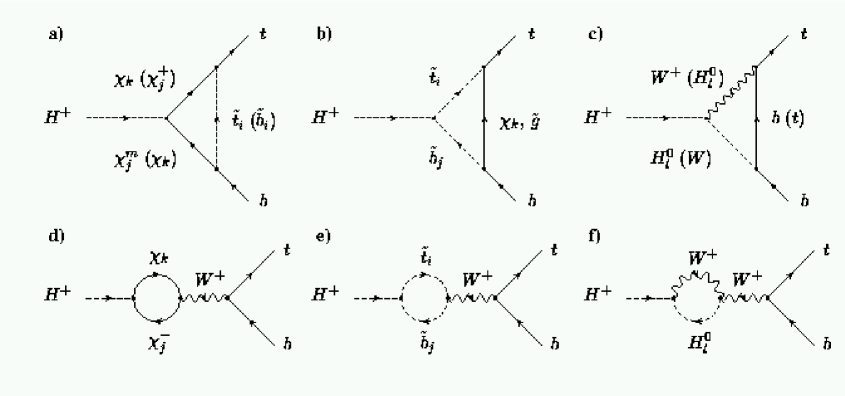
Figure 4.14: Sources of CP violation in $H^{+}\to t\bar{b}$ decays at the one-loop level in the MSSM with complex couplings ($i,j$ = 1, 2; $k$ = 1, …, 4; $l$ = 1, 2, 3)

Figure 4.15: CP violation in charged Higgs decays: (a) the asymmetry $\delta^{\rm CP}$ as a function of $m_{H^{+}}$ for selected values of $\phi_{t}$, assuming ${\rm tan}\beta$ = 10 and $\phi_{b}~{}=~{}0$, and (b) $\delta^{\rm CP}$ as a function of ${\rm tan}\beta$ for $m_{H^{+}}$ = 700 GeV and $\phi_{t}=\pi/2$. The other parameters are fixed by (4.16).

With $m_{H^{+}}$ = 700 GeV, taking the expected statistics of $e^{+}e^{-}\to H^{+}H^{-}\to t\bar{b}\bar{t}b$ at $\sqrt{s}$ = 3 TeV and assuming realistic charge tagging performances, a 3$\sigma$ effect would be observed with ${\cal{L}}$ = 5 ab^-1, for an asymmetry $|\delta^{\rm CP}|$ = 0.10.

4.3 Summary

The CLIC multi-TeV $e^{+}e^{-}$ linear collider has the potential to complete the study of the Higgs boson and to investigate an extended Higgs sector over a wide range of model parameters. Preserving the LC signature properties of clean events, with well-defined kinematics, will require a substantial effort of machine parameter optimization, detector design and data analysis techniques. However, exploratory studies, accounting for realistic experimental conditions, confirm that CLIC will perform precision measurements and push its sensitivity up to the kinematical limits.

While the main motivation for experimentation at a multi-TeV LC arises from the search for new phenomena beyond the Standard Model, as discussed in the following Chapters, CLIC’s role in studying the Higgs sector will also be crucial in completing the mapping of the $H^{0}$ boson profile. Table 4.5 summarizes the accuracies expected from some Clic measurements of the properties of a Higgs boson in the SM. Additionally, CLIC would have unique capabilities for studying heavy Higgs bosons in extended scenarios. In this way, the multi-TeV CLIC project will ensure the continuation of a competitive $e^{+}e^{-}$ physics programme via a second-generation project able to address deeper physics questions in the Higgs sector.

Table 4.5: Summary of expected accuracies on Higgs properties at CLIC with $\sqrt{s}$ = 3 TeV and 5 ab^-1 of luminosity

Parameter		$M_{H}$ (GeV)	$\delta X/X$
$\delta g_{Htt}/g_{Htt}$		120–180	0.05–0.10
$\delta g_{Hbb}/g_{Hbb}$		180–220	0.01–0.03
$\delta g_{H\mu\mu}/g_{H\mu\mu}$		120–150	0.03–0.10
$\delta g_{HHH}/g_{HHH}$		120–180	0.07–0.09
$g_{HHHH}$		120	$\neq$ 0 (?)

Chapter 5 SUPERSYMMETRY

Supersymmetry (SUSY) is one of the best-motivated theories beyond the Standard Model [1]. Not only is it theoretically elegant, providing a unified description of fermions and bosons, including matter particles and force carriers, but it is also potentially capable of connecting gravity with the other interactions, and appears an essential ingredient of string theory. From the phenomenological point of view, the most compelling feature of SUSY is that it stabilizes the Higgs mass against radiative corrections, provided the supersymmetric particles have masses $\tilde{m}\leq$ O(1) TeV [2]. The minimal supersymmetric extension of the Standard Model (MSSM) also predicts a light Higgs boson with $m_{h}\;\raisebox{-3.87495pt}{$\textstyle\stackrel{{\scriptstyle\textstyle<}}{{\sim}}$}\;$ 130 GeV [3], which is favoured by present precision electroweak data [4, 5]. Furthermore, unification of the Standard Model gauge couplings and electroweak symmetry breaking occur naturally in the MSSM as a result of renormalization-group (RG) evolution [6], and the lightest supersymmetric particle (LSP) is a good cold dark matter candidate, if SUSY appears within the TeV energy range [7].

In the MSSM, as well as two scalar partners for each quark and lepton, there are four neutralinos and two charginos as superpartners for the gauge and Higgs bosons. Moreover, there are five physical Higgs bosons, $h^{0}\!$, $H^{0}\!$, $A^{0}\!$, and $H^{\pm}\!$. If nature is indeed supersymmetric, it is likely that the LHC will have observed part of the spectrum by the time CLIC comes into operation. In addition, it is likely that a TeV-scale $e^{+}e^{-}$ linear collider (LC) will have made accurate measurements of some kinematically accessible states, as illustrated by the sample spectra in Fig. 5.1. However, to explore the theory fully, we will need to measure accurately the complete sparticle spectrum, just as we need measurements of the top quark and the Higgs boson to complete the Standard Model. We will need to determine all the MSSM masses, mixing angles, couplings, spins, etc., in order to

• determine all the soft SUSY-breaking parameters,

• test their unification at some high scale, which might be the GUT scale or
  the SUSY-breaking scale,

• pin down the SUSY-breaking mechanism, e.g. whether it is mediated by gravity,
  gauge interactions or anomalies,

• test the consistency of the model.

We also emphasize that the minimality of the MSSM is an assumption, which must be tested.

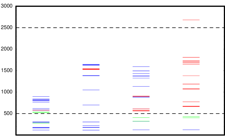
Figure 5.1: Examples of mass spectra of updated post-LEP benchmark points [8]. Sparticles that would be discovered at the LHC, a 1-TeV LC and CLIC are shown as blue, green and red lines, respectively. The kinematic reaches of a 1-TeV LC and CLIC at 5 TeV are shown as dashed lines.

The LHC has discovery potential for squarks and gluinos for masses up to about 2.5 TeV. However, its reach for neutralinos, charginos and sleptons is much lower, namely of the order of 0.5 TeV. We recall that the questions of unification of SUSY parameters and of the nature of SUSY breaking require that the measured parameters be extrapolated over many orders of magnitude, from 10³ GeV to 10¹⁶ GeV. Very accurate measurements are required in order to avoid large errors at the high scale, which needs the most precise measurements possible at an $e^{+}e^{-}$ collider, even of sparticles previously discovered at the LHC.

At CLIC, the clean experimental conditions of $e^{+}e^{-}$ annihilation at $\sqrt{s}$ = 3–5 TeV will enable us to make many such detailed measurements. Tunable energy and beam polarization will be powerful tools to disentangle various production channels, enhance signals, and reduce background processes. Tunable energy also allows for threshold scans, and polarization is vital to determine the quantum numbers, couplings, and mixing angles. A high luminosity of 1 ab^-1 per year is essential for precision measurements, and even higher energy or luminosity may be necessary for some particularly difficult scenarios. A multi-TeV $e^{+}e^{-}$ linear collider such as CLIC will thus be the ideal machine to complete the measurements of the LHC and a TeV-scale LC in order to fulfil the above tasks.

In the following, we discuss the potential of CLIC for studying heavy charginos, neutralinos, sleptons, and squarks. To this end, we use for reference a specific set of benchmark points in the CMSSM, a constrained version of the MSSM with universal soft SUSY-breaking parameters. We concentrate in particular on sparticles with masses beyond the reach of the LHC and a TeV-scale LC. We also discuss the determination of the underlying SUSY-breaking parameters and their extrapolation to the GUT scale, in order to test unification and to clarify the nature of SUSY breaking.

5.1 Post-LEP Benchmarks and the CLIC Reach

Benchmark scenarios provide helpful aids for better understanding the complementarity of different accelerators in the TeV energy range. A set of benchmark supersymmetric model parameters that are consistent with the constraints from LEP and other experiments, as well as the cosmology relic density, have been proposed in Ref. [9]. They were framed in the constrained version of the MSSM (CMSSM) with universal soft symmetry-breaking scalar masses $m_{0}$, gaugino masses $m_{1/2}$ and trilinear supersymmetry-breaking parameters $A_{0}$ at a high input scale, as expected in a minimal supergravity (mSUGRA) model of soft supersymmetry breaking. In this framework, the pseudoscalar Higgs mass $m_{A}$ and the Higgs mixing parameter $\mu$ (up to a sign) can be derived from the other MSSM parameters by imposing the electroweak vacuum conditions for any given value of $\tan\beta$. Thus, given the set of input parameters determined by $m_{1/2},m_{0},A_{0},\tan\beta$ and ${\rm sgn}(\mu)$, the entire spectrum of sparticles can be derived. For simplicity, the analysis was restricted to $A_{0}=0$.

These post-LEP benchmark scenarios have recently been updated [8], so as to respect the improved restrictions on the relic density of cold dark matter particles imposed by the WMAP measurements [10]. We summarize below some features of the updates mandated by WMAP. In the subsequent discussion, we use the updated post-WMAP benchmarks as far as possible, commenting on differences from the original set when necessary.

5.1.1 Benchmark Points

Details of the experimental constraints imposed on the CMSSM, the values of the parameters chosen as benchmark points, their justifications and the resulting sparticle spectra may be found in Refs.[9, 8].

Figure 5.2 displays most of the proposed CMSSM benchmark points, superimposed on the regions of the $(m_{1/2},m_{0})$ plane allowed by laboratory limits, particularly that from LEP on $m_{h}$, from $b\rightarrow s\gamma$, and cosmology. The original versions of the CMSSM benchmark points were chosen with a relic density in the range 0.1 $<\Omega_{\chi}h^{2}<$ 0.3 [9], but WMAP and previous data now prefer the more limited range 0.094 $<\Omega_{\chi}h^{2}<$ 0.129, corresponding to the narrow strips shown in Fig. 5.2. For most of the benchmark points, a small reduction in $m_{0}$ sufficed to relocate them on the WMAP strip for the corresponding value of $\tan\beta$ [8]. However, in some cases, notably benchmarks H and M, more substantial changes in $m_{0}$ and/or $m_{1/2}$ were made in order to accommodate the new WMAP constraint. Later, where relevant for specific sparticle analyses, we comment on the implications of these changes.

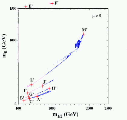
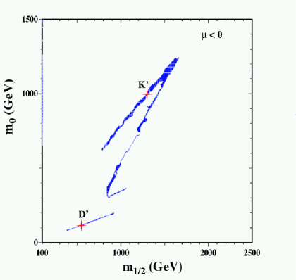
Figure 5.2: Overview of the updated proposed CMSSM benchmark points in the $(m_{0},m_{1/2})$ planes, superposed on the strips allowed by laboratory limits and the relic density constraint, for $\mu>$ 0 and $\tan\beta$ = 5, 10, 20, 35, 50, and for $\mu<$ 0 and $\tan\beta$ = 10, 35 [8]

The lightest supersymmetric particle would be charged in the bottom right dark-shaded triangular region, which is therefore excluded. The experimental constraints on $m_{h}$ and $b\rightarrow s\gamma$ exert pressures from the left, which depend on the value of $\tan\beta$ and the sign of $\mu$. The indication of a deviation from the Standard Model in $g_{\mu}-2$ disfavours $\mu<0$ at the 2$\sigma$ level. Large values of $m_{0}$ and $m_{1/2}$ for $\mu>0$ are disfavoured at the 1$\sigma$ level, as indicated by darker shading on parts of the WMAP lines. The improved WMAP constraint on the relic density has shrunk the previous ‘bulk’ region at low $m_{0}$ and $m_{1/2}$, and narrowed and shortened the coannihilation ‘tails’ extending to large $m_{1/2}$, which dominate Fig. 5.2. Not shown is the ‘focus-point’ region at large $m_{0}$ near the boundary of the region with proper electroweak symmetry breaking, where two more benchmark points are located.

The proposed benchmark points are not intended to sample the allowed CMSSM parameter space in a statistically unbiased way, but rather to span the essential range of theoretical possibilities, given our present knowledge. Estimates of the numbers of CMSSM particles accessible to different accelerators in the various proposed benchmark scenarios are summarized in Fig. 1.1 in the general introduction.

5.1.2 Detection at the LHC

In compiling Fig. 1.1, a preliminary inspection was made of the LHC potential for these benchmark points, based on the simulation results summarized in the ATLAS Technical Design Report [11] and in the CMS Note [12]. A detailed study is clearly required before a real assessment of the LHC physics potential for these benchmarks can be made, and both ATLAS and CMS have made more detailed studies of these and earlier benchmark scenarios. However, for this preliminary look, simplified assumptions were adopted to estimate the discovery potential of the LHC, assuming ATLAS and CMS combined, together with an integrated luminosity of 300 fb^-1 per experiment [9, 8]. We see in Fig. 5.3(a) how the number of MSSM particles detectable at the LHC varies along the WMAP line for $\tan\beta$ = 10, including the points B and C as special cases. For a more complete discussion of sparticle observability along WMAP lines, including other values of $\tan\beta$, see Ref. [8]. We see that the LHC can detect gluinos and all the squarks, for any allowed value of $m_{1/2}$, but may be expected to miss many sleptons, neutralinos, charginos and Higgs bosons, except in the lower part of the $m_{1/2}$ range.

Figure 5.3: Estimates of the numbers of MSSM particles that may be detectable as functions of $m_{1/2}$ along the WMAP line for $\mu>$ 0 and $\tan\beta$ = 10, for the LHC, a 0.5-TeV $e^{+}e^{-}$ linear collider, a 1-TeV $e^{+}e^{-}$ linear collider, and the latter combined with the LHC. The complementarity of the LHC and a linear collider emerge clearly. The locations of the benchmark points B^′ and C^′ along these WMAP lines are indicated, as is the nominal lower bound on $m_{1/2}$ imposed by $m_{h}$ (dashed lines) [8].

Thus, in the framework of the CMSSM, the open questions after the LHC might include completing the spectrum of electroweakly-interacting sparticles, as well as detailed measurements of the gluino and squarks, which will not be easy at the LHC.

5.1.3 Detection at Linear Colliders

Sparticles can generally be produced at any linear $e^{+}e^{-}$ collider (LC) if its centre-of-mass energy is larger than twice the mass of the sparticles, the pair-production threshold. Exceptions include heavier charginos and neutralinos, which can be produced in association with lighter charginos or neutralinos, respectively. Also, for sufficiently light neutralinos and sneutrinos, observation of the radiative production of otherwise invisible final states may be experimentally accessible.

Typical supersymmetric signals are multilepton final states and multijet ones with large missing transverse energy. Sneutrinos can be detected at threshold energies if they decay into channels including charged leptons with a sufficiently large branching ratio. For example, in some scenarios, the ${\tilde{\nu}}_{\tau}$ can decay into $\tau{\tilde{W}}$. A counter example to this possibility is the updated benchmark point B, where all the sneutrino decays are invisible. However, even in such a case, sneutrinos can be detected at higher energies via the decays of charginos.

For $e^{+}e^{-}$ linear colliders, data samples of the order of 1000 fb^-1 or more are expected to be collected over a period of several years. Apart from the threshold requirement to produce the particles, the product of the branching ratio times the unpolarized cross section for the detectable channels was required to be larger than 0.1 fb in order to observe the sparticle, leading to at least 100 produced sparticles in the total data sample.

We see in Fig. 5.3(b) that a 0.5-TeV $e^{+}e^{-}$ linear collider would already be able to fill in many of the gaps in the MSSM spectrum left by the LHC for smaller $m_{1/2}$. The reach of a 1-TeV $e^{+}e^{-}$ linear collider would be correspondingly greater, as seen in Fig. 5.3(c). Such a machine would be largely complementary to the LHC, as seen in Fig. 5.3(d).

5.1.4 Perspectives

Assuming that the LHC and an $e^{+}e^{-}$ linear collider in the range $\lappeq$ 1 TeV have been taking data for several years before the start of a 3 TeV machine like CLIC (CLIC3000), we infer that supersymmetry will most probably already have been discovered by that time, if it exists. Hence the primary rôle of CLIC may be to complete the sparticle spectrum, and disentangle and measure more precisely the properties of sparticles already observed at the LHC and/or a lower-energy $e^{+}e^{-}$ linear collider. However, a machine like CLIC would be needed even for the direct discovery of supersymmetry in the most problematic cases, such as benchmark scenarios H and particularly M, where no sparticles may be seen at either the LHC or a TeV-class LC, as seen in Fig. 1.1.

A few benchmark points emerge as typical of situations that could arise in the future.

• Point C has very low masses, and is representative also of points A, B, D, G, I, L. In these cases, the LHC would have discovered the $H^{\pm}$, as well as seen the $h^{0}$, and also the gauginos $\tilde{\chi}^{0}_{1}$, $\tilde{\chi}^{0}_{2}$ and $\tilde{\chi}^{\pm}_{1}$, the charged sleptons, the squarks and the gluino. A 1-TeV linear collider would enable the detailed study of the $h^{0}$ and of the same gauginos and sleptons, and it might discover the missing gauginos in some of the scenarios. However, one would require CLIC, perhaps running around 2 TeV, to complete the particle spectrum by discovering and studying the heavy Higgses and the missing gauginos. CLIC could also measure more precisely the squarks and in particular disentangle the left- and right-handed states and, to some extent, the different light squark flavours.

• Point J features intermediate masses, much like point K. Here, the LHC would have discovered all the Higgs bosons, the squarks and the gluino, but no gauginos or sleptons. The 1-TeV $e^{+}e^{-}$ linear collider would study in detail the $h^{0}$ and could discover the $\tilde{e}_{R}$, $\tilde{\mu}_{R}$ and $\tilde{\tau}_{1}$, but other sparticles would remain beyond its kinematic reach. CLIC3000 could then study in detail the heavy Higgses, as discussed in the previous chapter. It would also discover and study the gauginos and the missing sleptons, and even observe in more detail a few of the lighter squarks that had already been discovered at the LHC. However, to see the remaining squarks at a linear collider would require CLIC to reach slightly more than 3 TeV.

• Point E has quite distinctive decay characteristics, due to the existence of heavy sleptons and squarks. In this situation, the LHC would have discovered the $h^{0}$, all squarks and the gluino. The gauginos are in principle accessible, but their discovery may be made more difficult by their predominant decays into jets, contrary to the previous benchmark points, and sleptons would remain unobserved. At a 1-TeV $e^{+}e^{-}$ linear collider, the detailed study of the $h^{0}$ and of the gauginos could be undertaken. The discovery of the first slepton, actually a $\tilde{\nu}_{e}$, could be made at CLIC3000, which could also study the three lightest squarks. The discovery and analysis of the heavy Higgses would then require the CLIC energy to reach about 3.5 TeV, which would also allow the discovery of all sleptons and the observation of all squarks. A detailed analysis of the accuracy in the determination of the smuon mass at $\sqrt{s}$ = 3.8–4.2 TeV is presented later in this chapter.

• Point H has quite heavy states, as does scenario M. The LHC would only discover the $h^{0}$, all other states being beyond its reach, so the LHC might leave the existence of supersymmetry as an open question! At point H, a 1-TeV linear collider would discover the lighter $\tilde{\tau}$ and the LSP $\chi$, but no other sparticles. A 1-TeV linear collider would discover no sparticles at point M. However, CLIC at 3 TeV would be able to discover most of the gauginos and sleptons. The CLIC sensitivity to the smuon mass, using both a muon energy technique and a threshold scan, is discussed later. On the other hand, to discover all the squarks, $\ell^{+}\ell^{-}$ collisions in excess of 5 TeV would be needed. There is currently no $e^{+}e^{-}$ project aiming at such energies, and we recall that neutrino radiation would become a hazard for a $\mu^{+}\mu^{-}$ collider at such a high energy.

• Along the lines defined by the WMAP constraints, the reach in supersymmetric particles for a given collider and the phenomenology of their decays change significantly. As we discuss later, the CLIC reach for the dilepton decay signature of a heavier neutralino, $\chi_{2}\to\ell^{+}\ell^{-}\chi$ is significantly greater than that of the LHC or a 1-TeV linear collider. Additionally, we have chosen a point at $m_{1/2}$ = 750 GeV and $\tan\beta$ = 10 to study the potential accuracy in the determination of the mass of the sleptons and of the $\tilde{\chi}^{0}_{2}$. This point is located at the limit of the sensitivity of the LHC and of a 1-TeV linear collider for probing the heavy neutralinos and the slepton sectors, and represents the limit of the coverage of the full supersymmetric spectrum at CLIC at 3 TeV.

• As in the case of a 1-TeV $e^{+}e^{-}$ linear collider, a photon collider option for CLIC would extend the discovery range for heavy Higgs bosons. Additionally, it would allow one to discover all four Higgs bosons in scenarios E, H and M, for a 3-TeV collider, and also in F, for a 5-TeV collider. The detection of heavier MSSM Higgs bosons at a CLIC-based $\gamma\gamma$ collider is discussed in more detail in the previous section.

The corresponding estimates of the numbers of MSSM particles that can be detected are shown in Fig. 5.4. Beyond the discovery of sparticles, a crucial issue in the understanding of the nature of any new physics observed will be the accuracy obtainable in the determination of the sparticle masses and decays, and also their quantum numbers and mixing. A strong advantage of lepton colliders is the precision with which such sparticle properties can be measured. A strong advantage of lepton colliders is the precision with which such sparticle properties can be measured, as discussed in the next section of this chapter. Typically, the masses of sleptons and gauginos can be determined with a precision of a few per mille, by threshold scans and by measuring end-points of two-body decay channel signatures in inclusive distributions. This high precision, even for a limited number of sparticles, will be of cardinal importance for the reconstruction of the underlying supersymmetric model and exploration of the supersymmetry-breaking mechanism [13].

The availability of polarized beams at CLIC would, furthermore, provide additional tools for identifying supersymmetric particles and allow for additional measurements of parameters of the supersymmetric model, such as the mixing angles of the sparticles, as discussed later in this chapter.

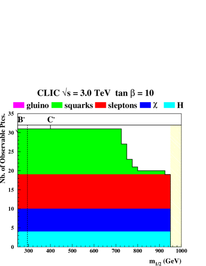
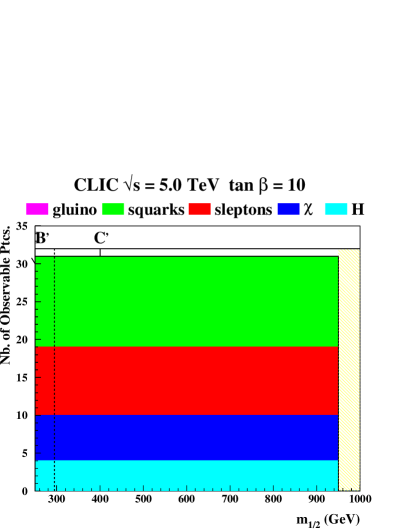
Figure 5.4: Estimates of the numbers of MSSM particles that may be detectable as functions of $m_{1/2}$ along the WMAP line for $\mu>$ 0 and $\tan\beta$ = 10, for CLIC operating at 3 TeV (left panel) and 5 TeV (right panel). The locations of the benchmark points B^′ and C^′ along these WMAP lines are indicated, as is the nominal lower bound on $m_{1/2}$ imposed by $m_{h}$ (dashed lines) [8].

5.1.5 Generalized Supersymmetric Models

We complete this introductory discussion by looking beyond specific CMSSM benchmark scenarios and WMAP lines, considering the prospects for observing supersymmetric particles at $e^{+}e^{-}$ colliders in more general scenarios that conserve $R$ parity. For this purpose, we display in Fig. 5.5 random samples of supersymmetric models, initially disregarding the cosmological relic-density constraint (red points) and subsequently including it (blue points). The plots feature the masses of the two lightest observable sparticles, namely the next-to-lightest supersymmetric particle (NSP) and the next-to-next-to-lightest supersymmetric particle (NNSP).

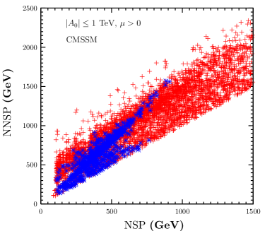
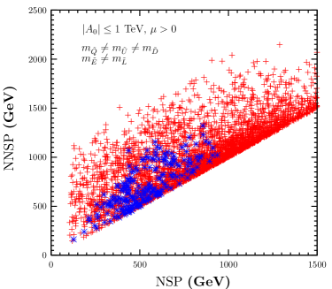
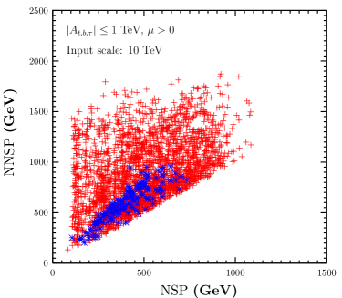
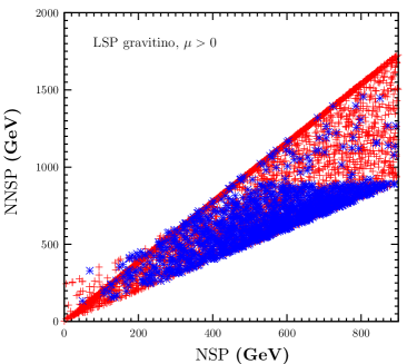
Figure 5.5: Scatter plots of the masses of the next-to-lightest supersymmetric particle (NSP) and the next-to-next-to-lightest supersymmetric particle (NNSP) for (a) the CMSSM, (b) models without squark and slepton mass universality, (c) universality for the squark and slepton masses separately but stability of the effective potential up to 10 TeV only, and (d) a gravitino LSP. Each scatter plot contains 50,000 points with $m_{\tilde{Q}},m_{\tilde{D}},m_{\tilde{U}},m_{\tilde{L}},m_{\tilde{E}},m_{1/2},m_{1},m_{2}<$ 2 TeV (where $m_{1,2}$ are the soft supersymmetry-breaking contributions to the Higgs boson masses), – 1 TeV $<A_{0}<$ 1 TeV, $\tan\beta<$ 58 and $\mu>$ 0. We thank Vassilis Spanos for supplying these figures

In order to make contact with the previous analysis, we first consider in panel (a) of Fig. 5.5 the CMSSM with parameters chosen to obey the standard experimental (and cosmological) constraints. We then consider in panel (b) models in which no universality is assumed for the squark and slepton masses, subject to the supplementary constraint that the effective potential remain stable when the theory is extrapolated up to the GUT scale, using the renormalization-group equations (RGEs). Panel (c) assumes universality for the squark and slepton masses separately, but stability is required only for RGE evolution up to 10 TeV. Finally, panel (d) is for models in which the LSP is assumed to be a gravitino.

In each case, we have generated 50,000 points with $m_{\tilde{Q}},m_{\tilde{D}},m_{\tilde{U}},m_{\tilde{L}},m_{\tilde{E}},m_{1/2},m_{1},m_{2}<$ 2 TeV (where $m_{1,2}$ are the soft supersymmetry-breaking contributions to the Higgs boson masses), – 1 TeV $<A_{0}<$ 1 TeV, $\tan\beta<$ 58 and $\mu>$ 0 (the plots for $\mu>$ 0 are not very different). The upper limits on the soft supersymmetry-breaking parameters are somewhat arbitrary, and one could argue that a varying measure related to the amount of hierarchical fine-tuning should be applied. However, we do note that the range considered contains comfortably most points allowed by the cosmological relic-density constraint.

We see that CLIC with $E_{c.m.}$ = 3 TeV would observe both the NSP and the NNSP in most cases, and CLIC with $E_{c.m.}$ = 5 TeV would observe them both in all the cases considered.

5.1.6 Alternative Benchmark Scenarios

Apart from the points discussed in Ref. [8] several other groups have recently proposed benchmark points for SUSY studies. For example, in Ref.  [14] a number of mSUGRA benchmark points similar to the ones discussed in [8] are proposed. Since these points were conceived at the Snowmass workshop in 2001, these benchmark points are often referred to as the Snowmass points (SPS points). In addition, points generated with different SUSY-breaking mechanisms are proposed: two points from a gauge-mediated SUSY-breaking scenario (GMSB), and from an anomaly-mediated SUSY-breaking scenario (AMSB). Both GMSB points have heavy squarks and gluinos, which are beyond the reach of a 1 TeV LC, but within reach of CLIC. For the second GMSB point also the heavy Higgses are beyond the reach of a 1 TeV LC (and even the LHC). The AMSB point chosen has many sparticles with a mass around or above 1 TeV: several gauginos, the heavy Higgses and all coloured sparticles. All these sparticles are, however, within the reach of a 3 TeV CLIC.

An alternative set of ‘string-inspired’ benchmark points, are given in Ref. [15]. These points are chosen such that there are always a few light sparticles which could possibly be detected at the Tevatron. However, each of these proposed benchmark scenarios always has a large number of sparticles in the TeV mass range and can be studied by CLIC. In some cases the masses are so large that even CLIC will not be able to see the full sparticle spectrum. In some of these scenarios only a few gauginos are accessible at a 1-TeV LC, and the sleptons and Heavy Higgses can only be studied at CLIC.

In all, these benchmark points, in scenarios different from mSUGRA, all seem to indicate that there is a role for CLIC to complete the sparticle spectrum.

5.2 Slepton and Squark Mass Determination

5.2.1 Smuon Mass Determination

A study has been performed of the reaction $e^{+}e^{-}\to\tilde{\mu}_{L}\tilde{\mu}_{L}\to\mu^{+}\tilde{\chi}^{0}_{1}\mu^{-}\tilde{\chi}^{0}_{1}$ at CLIC. The three main sources of background, also leading to two muons plus missing energy, are i) $e^{+}e^{-}\to W^{+}W^{-}\to\mu^{+}\mu^{-}\nu_{\mu}\bar{\nu}_{\mu}$, ii) $e^{+}e^{-}\to W^{+}W^{-}\bar{\nu}\nu\to\mu^{+}\mu^{-}\nu_{\mu}\bar{\nu}_{\mu}\nu_{e}\bar{\nu}_{e}$ and iii) $e^{+}e^{-}\to\tilde{\chi}^{0}_{1}\tilde{\chi}^{0}_{2},~{}\tilde{\chi}^{0}_{2}\tilde{\chi}^{0}_{2}\to\mu^{+}\mu^{-}\nu\bar{\nu}\tilde{\chi}^{0}_{1}\tilde{\chi}^{0}_{1}$. These backgrounds can be suppressed by requiring central production and decay kinematics compatible with those characteristic of smuon pair production. A multidimensional discriminant based on $M_{\mu\mu}$, $M_{\rm recoil}$, $E_{\rm missing}$, $\mu\mu$ acolinearity, $|\cos\theta_{\rm thrust}|$, $E_{t}$ and $E_{\rm hem}$ has been applied. The signal efficiency is flat with the muon energy.

5.2.1.1 The energy distribution method for mass determination

If the centre-of-mass energy $\sqrt{s}$ is significantly larger than twice the sparticle mass $M_{\tilde{\mu}}$, the latter can be determined by an analysis of the energy spectrum of the muon emitted in the two-body $\tilde{\mu}\rightarrow\tilde{\chi}^{0}_{1}\mu$ decay, as seen in Fig. 5.6. The two end-points, $E_{\rm min}$ and $E_{\rm max}$, of the spectrum are related to the $\tilde{\mu}$ and $\tilde{\chi}^{0}_{1}$ masses and to the $\tilde{\mu}$ boost by:

$$E_{\rm{max/min}}=\frac{M_{\tilde{\mu}}}{2}\,\left(1-\frac{M^{2}_{\tilde{\chi}^{0}_{1}}}{M^{2}_{\tilde{\mu}}}\right)\times\left(1\pm\sqrt{1-\frac{M^{2}_{\tilde{\mu}}}{E^{2}_{\rm beam}}}\right)$$ (5.1)

from which either the smuon mass $M_{\tilde{\mu}}$ can be extracted, if $M_{\tilde{\chi}^{0}_{1}}$ is already known, or both masses can be simultaneously fitted.

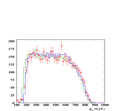
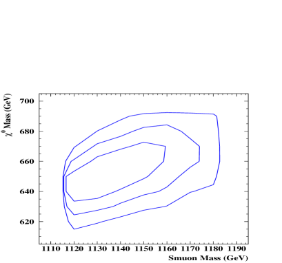
Figure 5.6: Left panel: Muon energy spectrum in the decay $\tilde{\mu}_{L}\to\mu\tilde{\chi}^{0}_{1}$ for the benchmark point H, corresponding to $M_{\tilde{\mu}_{L}}$ = 1150 GeV and $M_{\tilde{\chi}^{0}_{1}}$ = 660 GeV, as obtained for $\sqrt{s}$ = 3 TeV, assuming the baseline CLIC luminosity spectrum. Right panel: Accuracy in the determination of the $\tilde{\mu}_{L}$ and $\tilde{\chi}^{0}_{1}$ masses by a two-parameter fit to the muon energy distribution. The lines give the contours at 1$\sigma$, 68% and 95% C.L. for 1 ab^-1 of data at $\sqrt{s}$ = 3 TeV.

This technique, considered for the determination of squark masses at a 500-GeV LC in Ref. [16], has already been applied to sleptons for the LHC [11, 17] and a TeV-class LC [18]. It is interesting to consider its implications for the required momentum resolution in the detector. Two values of the solenoidal magnetic field $B=$ 4 and 6 T have been tested, corresponding to momentum resolutions $\delta p/p^{2}$ of 4.5 $\times$ 10^-5 and 3.0 $\times$ 10^-5 GeV^-1 respectively. No appreciable difference on the resulting mass accuracy has been found for these two momentum resolutions. This reflects the fact that, at CLIC, the main issue is the significant beamstrahlung smearing of the luminosity spectrum, and thus of the effective $E_{\rm beam}$ value. The corresponding effect has been estimated by assuming both a perfectly well known and constant beam energy and the smearing corresponding to the baseline CLIC parameters at a nominal $\sqrt{s}$ = 3 TeV. Results are summarized in Table 5.1 for the original version of benchmark point H. Since the updated post-WMAP version of point H has smaller $m_{1/2}$ and $m_{0}$, it would present a lesser experimental challenge.

Table 5.1: Results of a one-parameter $\chi^{2}$ fit to the muon energy distribution for benchmark point H, obtained under different assumptions on the $\delta p/p^{2}$ momentum resolution and the beamstrahlung spectrum. Accuracies are given for an integrated luminosity of 1 ab^-1.

$\delta p/p^{2}$		Beamstrahlung	Fit result (GeV)
0		none	1150 $\pm$ 10
3.0 $\times$ 10-5		none	1150 $\pm$ 12
4.5 $\times$ 10-5		none	1151 $\pm$ 12
4.5 $\times$ 10-5		standard	1143 $\pm$ 18

The smuon mass has been extracted by a $\chi^{2}$ fit to the muon energy spectrum by fixing $M_{\tilde{\chi}^{0}_{1}}$ to its nominal value (see Table 5.1). The fit has been repeated, leaving both masses free and performing a simultaneous two-parameter fit. The results are $M_{\tilde{\mu}_{L}}$ = (1145 $\pm$ 25) GeV and $M_{\chi^{0}_{1}}$ = (652 $\pm$ 22) GeV (see Fig. 5.6).

5.2.1.2 The threshold scan method for mass determination

An alternative method to determine the $\tilde{\mu}_{L}$ mass is an energy scan of the rise of the $e^{+}e^{-}\rightarrow\tilde{\mu}_{L}^{+}\tilde{\mu}_{L}^{-}$ cross section close to its kinematical threshold. It has been shown that an optimal scan consists of just two energy points, sharing the total integrated luminosity in equal fractions and chosen at locations optimizing the sensitivities to the $\tilde{\mu}_{L}$ width and mass, respectively [19]. Including the beamstrahlung effect induces a shift of the positions of the maxima in mass sensitivity towards higher nominal $\sqrt{s}$ energies (see Fig. 5.7). For benchmark point E (considering once again the pre-WMAP version), the cross section at $\sqrt{s}$ = 3 TeV is too small for an accurate measurement. A higher centre-of-mass energy, 4 TeV, and polarized beams need to be considered. By properly choosing the beam polarization, not only are the pair-production cross sections increased (as discussed in a later section of this chapter), but also their sensitivities to the smuon masses. Results are summarized in Table 5.2. In the case of point H (also in the pre-WMAP version), we see that a mass resolution $\delta M$ = 15 GeV is attained, which increases to 36 GeV for point E. However, polarized beams would, in that case, reduce $\delta M$ to 22 MeV.

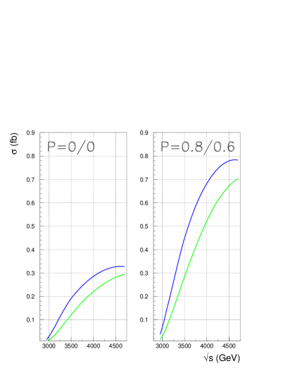
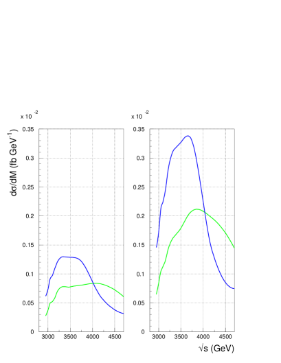
Figure 5.7: Smuon mass determination with threshold scans. Left: cross section as a function of $\sqrt{s}$ for smuon pair production with and without beam polarization. The curves indicate the effect of the luminosity spectrum on the rise of the cross section. Right: cross section $\sigma$ sensitivity to the smuon mass $M$ indicated in terms of $d\sigma/dM$ as a function of centre-of-mass energy $\sqrt{s}$, showing the optimal energy point for the threshold scan. Again the two panels are for no beam polarization and for 80/60% polarization, and the two curves show the effect of the CLIC luminosity spectrum.

Table 5.2: Accuracies in the determinations of the smuon masses for the two benchmark scenarios considered in this study, using threshold scans with different experimental conditions

Point	Beam-	Pol.	$\sqrt{s}$	$\int{\cal{L}}$	$\delta M$
	strahlung		(TeV)	(ab-1)	(GeV)
H	none	0/0	3.0–3.5	1	$\pm$ 11
H	standard	0/0	3.0–3.5	1	$\pm$ 15
E	none	0/0	3.8–4.2	1	$\pm$ 29
E	standard	0/0	3.8–4.2	1	$\pm$ 36
E	none	80/60	3.8–4.2	1	$\pm$ 17
E	standard	80/60	3.8–4.2	1	$\pm$ 22

5.2.2 Analysis of Stop Squarks

The scalar partners of the top quark (stops), $\tilde{t}_{\rm L}$ and $\tilde{t}_{\rm R}$, are of particular interest among the squarks. Owing to their large Yukawa coupling, they play an important role in the renormalization group (RG) evolution and in the radiative corrections to the lightest Higgs mass. Moreover, the $\tilde{t}_{\rm L}$ and $\tilde{t}_{\rm R}$ mix to mass eigenstates $\tilde{t_{1}}~{}=~{}\tilde{t}_{\rm L}\cos\theta_{\tilde{t}}+\tilde{t}_{\rm R}\sin\theta_{\tilde{t}}$ and $\tilde{t_{2}}=\tilde{t}_{\rm R}\cos\theta_{\tilde{t}}-\tilde{t}_{\rm L}\cos\theta_{\tilde{t}}$, where $\theta_{\tilde{t}}$ is the stop mixing angle. This mixing also leads to a sizeable mass splitting of $\tilde{t_{1}}$ and $\tilde{t_{2}}$, which contrasts with the near-degeneracy of the squarks $\tilde{q}_{\rm L,R}$ of the first and second generations. The masses of the stops are given by

$${\rm diag}(m_{\tilde{t_{1}}},\,m_{\tilde{t_{2}}})=R^{\tilde{t}}\left(\!\!\begin{array}[]{cc}m_{\tilde{t}_{\rm L}}^{2}&(A_{t}-\mu\cot\beta)\,m_{t}\\ (A_{t}-\mu\cot\beta)\,m_{t}&m_{\tilde{t}_{\rm R}}^{2}\end{array}\!\!\right)(R^{\tilde{t}})^{\dagger}\,,$$ (5.2)

where $A_{t}$ is the trilinear stop–Higgs coupling, $R^{\tilde{t}}$ is the stop mixing matrix

$$R^{\tilde{t}}=\left(\!\!\begin{array}[]{rr}\cos\theta_{\tilde{t}}&\sin\theta_{\tilde{t}}\\ -\sin\theta_{\tilde{t}}&\cos\theta_{\tilde{t}}\end{array}\!\!\right)\,,$$ (5.3)

and $m_{\tilde{t_{1}}}<m_{\tilde{t_{2}}}$ by convention. As already mentioned, stops play an important role in the RG running. For the extrapolation to the GUT scale discussed later in this chapter, it is thus essential to know their parameters as precisely as possible. At the LHC, stop masses may be measured with errors of a few per cent, but measuring $\theta_{\tilde{t}}$ and $A_{t}$ will hardly be possible. In $e^{+}e^{-}$ collisions, however, measurements of the products of cross sections with branching ratios (especially with polarized beams), threshold scans and kinematical distributions may be used to determine $m_{\tilde{t_{1}}}$, $m_{\tilde{t_{2}}}$, $\theta_{\tilde{t}}$ and $A_{t}$ quite precisely.

Figure 5.8 shows cross sections for $e^{+}e^{-}\to\tilde{t}_{i}\bar{\tilde{t}_{i}}\,$ ($i$ = 1, 2) for $m_{\tilde{t_{1}}}$ = 1 TeV, $m_{\tilde{t_{2}}}$ = 1.3 TeV and $\theta_{\tilde{t}}$ = 70^∘ as functions of $\sqrt{s}$ for unpolarized beams. Supersymmetric QCD corrections [20] and initial-state radiation (ISR) are included. The cross sections show characteristic dependences [21] on the mixing angle and on beam polarization. Measurements with different polarizations may thus be used to determine $\theta_{\tilde{t}}$. Figure 5.9 shows polarized cross sections for $\tilde{t_{1}}\,\bar{\tilde{t_{1}}}$ and $\tilde{t_{2}}\,\bar{\tilde{t_{2}}}$ production normalized to the unpolarized ones, $\sigma^{\rm pol}/\sigma^{\rm unpol}$, as functions of the electron beam polarization $P_{e^{-}}$ and the stop mixing angle. Positron polarization is assumed to be zero, but could be used to enhance further the dependence on $\theta_{\tilde{t}}$.

Figure 5.8: Cross Sections for stop pair production for $m_{\tilde{t_{1}}}$ = 1 TeV, $m_{\tilde{t_{2}}}$ = 1.3 TeV, $\theta_{\tilde{t}}$ = 70^∘ and $m_{\tilde{g}}$ = 750 GeV

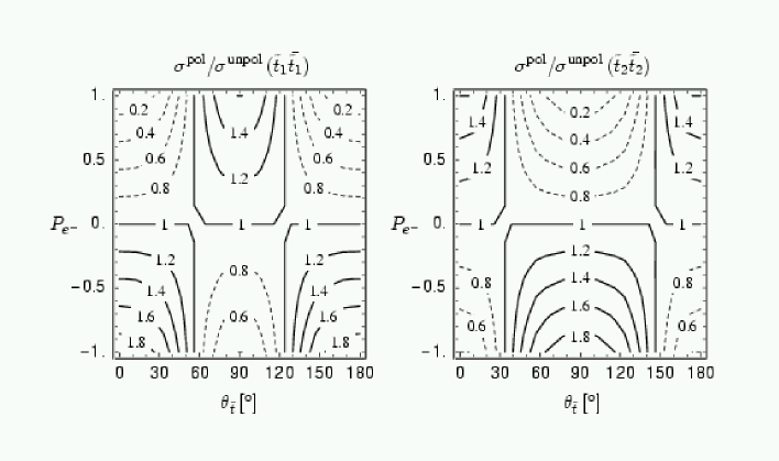
Figure 5.9: Polarized cross sections for $\tilde{t_{1}}\bar{\tilde{t_{1}}}$ and $\tilde{t_{2}}\bar{\tilde{t_{2}}}$ production normalized to the unpolarized ones, $\sigma^{\rm pol}/\sigma^{\rm unpol}$, as functions of the electron beam polarization $P_{e^{-}}$ and the stop mixing angle $\theta_{\tilde{t}}$, for $m_{\tilde{t_{1}}}$ = 1 TeV, $m_{\tilde{t_{2}}}$ = 1.3 TeV and $\sqrt{s}$ = 3 TeV. The positron beam polarization has been assumed to vanish.

If both stop masses and the mixing angle are measured, and $\tan\beta$ and $\mu$ are known from, for example, the chargino/neutralino sector, $A_{t}$ can be determined by

$$A_{t}=\frac{1}{2m_{t}}\left(m_{\tilde{t_{1}}}^{2}-m_{\tilde{t_{2}}}^{2}\right)\sin 2\theta_{\tilde{t}}+{\mu\over\tan\beta}\,.$$ (5.4)

This can then be compared with indirect estimates of $A_{t}$ from precision measurements of $m_{h}$ [22]. It is also possible to determine $A_{t}$ via the associated production of stops with Higgs bosons [23] (which has, however, a very small cross section at CLIC energies) and/or from $\tilde{t_{2}}\to\tilde{t_{1}}\,(h^{0}\!,H^{0}\!,A^{0})$ and $\tilde{b}_{i}H^{+}$ decays [24], which can have large branching ratios if $A_{t}$ and/or $\mu$ are large.

5.3 Neutralino Mass Determination

Operating at 3 to 5 TeV with large luminosity, CLIC will be able to improve significantly on the reach for heavy neutralinos, beyond the anticipated LHC sensitivity. A general study of the prospective CLIC sensitivity has been carried out, including a simulation of the detector response parametrized by the SIMDET program. Inclusive chargino and neutralino pair production have been analysed to determine the sensitivity obtainable from the dilepton invariant mass spectrum. The decay chains $\tilde{\chi}^{0}_{j}\to\ell^{\pm}\tilde{\ell}^{\mp}\to\ell^{+}\ell^{-}\tilde{\chi}^{0}_{1}$ and $\tilde{\chi}^{0}_{j}\to\tilde{\chi}^{0}_{i}Z^{0}\to\tilde{\chi}^{0}_{i}\ell^{+}\ell^{-}$ give rise to an excess of events in the $\ell^{+}\ell^{-}$ mass spectrum corresponding to the phase space for the cascade two-body decay of the first process or to the $Z^{0}$ mass peak in the second. A full scan of the $(m_{1/2},\;m_{0})$ plane has been carried out, using PYTHIA 6.21 interfaced to ISAJET 7.64. Events with at least two leptons and significant missing energy have been selected. Both SUSY backgrounds involving sleptons and SM gauge-boson pair production have been considered. Combinatorial backgrounds have been subtracted by taking the difference of the pair $e^{+}e^{-}+\mu^{+}\mu^{-}$ events and the mixed $e^{\pm}\mu^{\mp}$ events, and a sliding window has been used to search for an excess of 5 standard deviations or more of events in the $M_{\ell\ell}$ mass distribution. Results are shown in Figure 5.10 for $\tan\beta$ = 10, where the extended reach provided by CLIC is manifest. At larger values of $\tan\beta$, decays into $\tilde{\tau}$ become more significant, requiring a more detailed study, which must include $\tau$-lepton reconstruction.

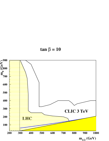
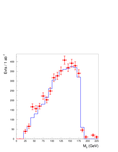
Figure 5.10: Left panel: The sensitivity to $\tilde{\chi}^{0}_{2}$ production at CLIC for $\sqrt{s}$ = 3 TeV compared with that of the LHC. Right panel: Dimuon spectrum measured at CLIC, assuming $m_{0}$ = 150 GeV, $m_{1/2}$ = 700 GeV and $\tan\beta$ = 10, used to derive the particle masses as discussed in the text.

To verify the CLIC capability for measuring the masses of heavy neutralinos, a representative point has been chosen at $m_{0}$ = 150 GeV, $m_{1/2}$ = 700 GeV and $\tan\beta$ = 10, which is compatible with the constraint on cold dark matter from the WMAP data and has $M_{\tilde{\chi}^{0}_{2}}$ = 540 GeV, $M_{\tilde{\chi}^{0}_{1}}$ = 290 GeV and $M_{\ell_{L}}$ = 490 GeV.

The dilepton invariant mass distribution shows a clear upper edge at 120 GeV, due to $\tilde{\chi}^{0}_{2}\to\mu^{\pm}\tilde{\mu}^{\mp}_{L}\to\mu^{+}\mu^{-}\tilde{\chi}^{0}_{1}$, which can be very accurately measured, already with 1 ab^-1 of data. However, in order to extract the mass of the $\tilde{\chi}^{0}_{2}$ state, the masses of both the $\tilde{\mu}_{L}$ and $\tilde{\chi}^{0}_{1}$ need to be known. As already discussed, a two-parameter fit to the muon energy distribution yields the masses of the $\tilde{\mu}_{L}$ and $\tilde{\chi}^{0}_{1}$ with accuracies of 3% and 2.5% respectively, using 1 ab^-1 of data. An improved accuracy can be obtained with higher luminosity and using also a threshold energy scan. We therefore assume that these masses can be known to 1.7% and 1.5% respectively, which gives an uncertainty of 8 GeV, or 1.6%, on the $\tilde{\chi}^{0}_{2}$ mass, when accounting for correlations. This uncertainty is dominated by that in the $\tilde{\mu}_{L}$ and $\tilde{\chi}^{0}_{1}$ masses. The accuracy in the determination of the end-point would correspond to a $\tilde{\chi}^{0}_{2}$ mass determination of 0.3 GeV, fixing all other masses, and is not sensitive to the details of the beamstrahlung and accelerator-induced backgrounds.

Last but not least, at CLIC with 3 TeV also the heavier $\tilde{\chi}^{0}_{3}$ and $\tilde{\chi}^{0}_{4}$ are accessible in this scenario and can be detected via the decays $\tilde{\chi}^{0}_{3}\to\tilde{\chi}^{0}_{1,2}Z^{0}$ and $\tilde{\chi}^{0}_{4}\to\tilde{\chi}^{0}_{1,2}h^{0}$.

5.4 Gluino Sensitivity in $\gamma\gamma$ Collisions

Measurements of the mass and coupling of the gluino pose some difficulties in $e^{+}e^{-}$ collisions, since the gluino couples only to strongly-interacting particles and is thus produced only at the one-loop level or in multiparton final states. In a recent publication, gluino pair production through triangular quark/squark loops in $e^{+}e^{-}$ annihilation with energies up to 1 TeV was investigated [25]. Owing to the large cancellation effects, it was found that promisingly large cross sections can only be expected for scenarios with large left-/right-handed up-type squark mass splittings, or with large top-squark mixing and for gluino masses up to 500 GeV. Small gluino masses of 200 GeV might be measured with a precision of about 5 GeV in centre-of-mass energy scans with luminosities of 100 fb^-1 per point.

Here we assume that CLIC can provide electron (positron) beam polarization of 80% (60%) and an integrated luminosity of 1000 fb^-1 per year. We compare the generally small production rates in $e^{+}e^{-}$ annihilation to the larger ones in photon–photon collisions. Further details on gluino pair production in high-energy photon collisions can be found in Ref. [26]. In the photon–photon collider version of CLIC, discussed in Section 2.6, 100%-polarized laser photons are backscattered from two electron beams, whose helicities must be opposite to those of the laser photons in order to maximize the number of high-energy photons. In the strong fields of the lasers, the electrons (or high-energy photons) can interact simultaneously with several laser photons. This non-linear effect increases the threshold parameter for $e^{+}e^{-}$ pair production to $X=(2+\sqrt{8})(1+\xi^{2})\simeq$ 6.5, which corresponds to laser wavelengths of 4.4 $\mu$m at an $e^{+}e^{-}$ centre-of-mass energy of 3 TeV [27]. The maximal fractional energy of the high-energy photons is then $x_{\max}=X/(X+1)\simeq$ 0.87. Since the low-energy tail of the photon spectrum is neither useful nor well understood, we use only the high-energy peak with $x>0.8\,x_{\max}$ = 0.69 and normalize our cross sections such that the expected number of events can be obtained through simple multiplication with the envisaged photon–photon luminosity of 100–200 fb^-1 per year. This requires reconstruction of the total final-state energy, which may be difficult because of the missing energy carried away by the escaping lightest SUSY particles (LSPs). However, high-energy photon collisions allow for cuts on the relative longitudinal energy in addition to the missing-$E_{T}$ plus multi-jet, top or bottom (s)quark, and/or like-sign lepton analyses performed at hadron colliders, and (in $R$-violating scenarios) sufficiently long-lived gluinos can be identified by their typical $R$-hadron signatures.

We adopt the current mass limit $m_{\tilde{g}}\geq$ 200 GeV from CDF [28] and D0 [29] searches in the jets- with-missing-energy channel, relevant to non-mixing squark masses $m_{\tilde{Q}}\geq$ 325 GeV and $\tan\beta$ = 3. Since values for the ratio of the Higgs vacuum expectation values $\tan\beta<$ 2.4 are already excluded by the LEP experiments, and since values between 2.4 and 8.5 are only allowed in a very narrow window of light Higgs boson masses between 113 and 127 GeV [30], we employ a safely high value of $\tan\beta$ = 10. For a conservative comparison of the $\gamma\gamma$ and $e^{+}e^{-}$ options at CLIC, we maximize the $e^{+}e^{-}$ cross section by adopting the smallest allowed universal squark mass $m_{\tilde{Q}}\simeq m_{\rm SUSY}$ = 325 GeV and large top-squark mixing with $\theta_{\tilde{t}}$ = 45.195^∘, $m_{\tilde{t_{1}}}$ = 110.519 GeV, and $m_{\tilde{t_{2}}}$ = 505.689 GeV, which can be generated by choosing appropriate values for the Higgs mass parameter, $\mu$ = –500 GeV, and the trilinear top-squark coupling, $A_{t}$ = 648.512 GeV [31]. The SUSY one-loop contributions to the $\rho$ parameter and the light top-squark mass $m_{\tilde{t_{1}}}$ are then, respectively, still significantly below and above the LEP limits, $\rho_{\rm SUSY}<$ 0.0012${}^{+0.0023}_{-0.0014}$ and $m_{\tilde{t_{1}}}\geq$ 100 GeV [32, 33]. For small values of $\tan\beta$, mixing in the bottom-squark sector remains small, and we take $\theta_{\tilde{b}}$ = 0^∘. A full set of Feynman diagrams can be generated and evaluated with the computer algebra packages FeynArts [34] and FormCalc [35].

Figure 5.11 shows a comparison of the total cross sections expected in $e^{+}e^{-}$ annihilation and $\gamma\gamma$ collisions for gluino masses between 200 and 500 GeV. Despite its maximization, the $e^{+}e^{-}$ cross section stays below 0.1 fb and falls steeply with $m_{\tilde{g}}$, so that gluino pair production will be unobservable for $m_{\tilde{g}}>$ 500 GeV, irrespective of the collider energy. In contrast, the $\gamma\gamma$ cross section reaches around 10 fb for a wide range of $m_{\tilde{g}}$. In $e^{+}e^{-}$ annihilation the gluinos are produced in a $P$ wave and the cross section rises rather slowly, whereas in $\gamma\gamma$ collisions they can be produced as an $S$ wave and the cross section rises much faster.

Figure 5.11: Gluino pair-production cross sections in $e^{+}e^{-}$ annihilation (left) and $\gamma\gamma$ collisions (right) as functions of the $e^{\pm}e^{-}$ centre-of-mass energy, for various gluino masses. The photon–photon luminosity has been normalized to unity in the high-energy peak.

The different threshold behaviours can be observed even more clearly in Fig. 5.12,

Figure 5.12: Sensitivity of the $e^{+}e^{-}$ annihilation (left) and $\gamma\gamma$ collision cross section (right) to the mass of the pair-produced gluino. The photon–photon luminosity has been normalized to unity in the high-energy peak.

where the sensitivities of $e^{+}e^{-}$ and $\gamma\gamma$ colliders to the gluino mass are compared. For the LHC experiments, a precision of $\pm$ 30…60 (12…25) GeV is expected for gluino masses of 540 (1004) GeV [36, 37]. If the masses and mixing angle(s) of the top (and bottom) squarks are known, a statistical precision of $\pm$ 5…10 GeV can be achieved in $e^{+}e^{-}$ annihilation for $m_{\tilde{g}}$ = 200 GeV for an integrated luminosity of 100 fb^-1 per centre-of-mass energy point. A precision of $\pm$ 2…5 GeV may be obtained at a CLIC photon collider for $m_{\tilde{g}}$ = 540 GeV and an integrated photon–photon luminosity of 50 fb^-1 per point, provided that the total final-state energy can be sufficiently well reconstructed. Of course, uncertainties from a realistic photon spectrum and the detector simulation should be added to the statistical error.

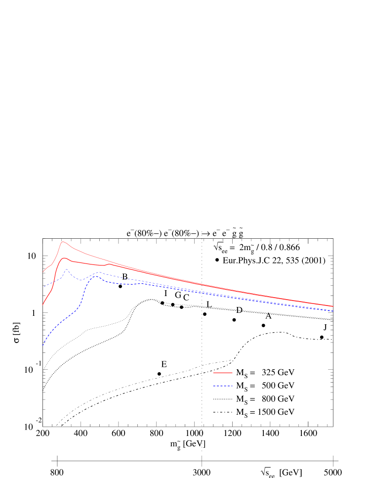
Figure 5.13: Dependence of the gluino pair-production cross section in $\gamma\gamma$ collisions on the universal squark mass $m_{\rm SUSY}$ for no squark mixing (thick curves) and maximal top-squark mixing (thin curves). The photon–photon luminosity has been normalized to unity in the high-energy peak. Also shown are the cross sections for the pre-WMAP versions of the supersymmetric benchmark points of Ref. [38].

Finally, we demonstrate in Fig. 5.13 that gluino pair production in $\gamma\gamma$ collisions depends only weakly on the universal squark mass $m_{\rm SUSY}$, and even less on the top-squark mixing. This is in sharp contrast to the results obtained in $e^{+}e^{-}$ annihilation [25]. In this plot, the $e^{+}e^{-}$ or $e^{-}e^{-}$ centre-of-mass energy is chosen close to the threshold for gluino pair production and is varied simultaneously with $m_{\tilde{g}}$. Also shown in Fig. 5.13 are several of the post-LEP supersymmetric benchmark points, considered here in their pre-WMAP versions [38]. We expect similar results for most of the post-WMAP versions, since they have similar values of $m_{1/2}$ [8]. Studies similar to those performed in Fig. 5.12 show that, with the exception of point E, where only about ten events per year are to be expected, the gluino mass can be determined with a precision of $\pm$ 20 GeV (as at point J) or better.

In summary, the determination of the gluino mass and coupling will be difficult in $e^{+}e^{-}$ collisions since the gluino couples only strongly and its pair-production cross section suffers from large cancellations in the triangular quark/squark loop diagrams. A photon collider may therefore be the only way to obtain precise gluino mass determinations and visible gluino pair production cross sections for general squark masses, and would thus strongly complement the physics programme feasible in $e^{+}e^{-}$ annihilation.

5.5 Reconstructing High-Scale SUSY Parameters

If LHC measurements of the MSSM spectrum are complemented by high-precision measurements at a prospective LC with sufficiently high energy, one can try to reconstruct the original theory at the high scale in a model-independent way, as shown in Refs. [13, 39]. We first summarize the procedure used, referring to Refs. [13, 39, 40] for further details.

We take the masses and cross sections of a particular point in SUSY parameter space together with their expected experimental errors from the LHC, a $\sqrt{s}$ = 800 GeV LC of the TESLA design [41] and a 4-TeV LC of the CLIC design. We assume that electrons can be polarized to 80% and positrons to 40% at the LCs. We then fit the underlying SUSY-breaking parameters at the electroweak symmetry-breaking scale, $Q_{\rm EWSB}=\sqrt{m_{\tilde{t}_{1}}m_{\tilde{t}_{2}}}$, to these observables. An initial set of parameters is obtained by inverting tree-level formulas for masses and cross sections. This set serves as a starting point for the fit, which is carried out with MINUIT [42] to obtain the complete correlation matrix. In the fit, the complete spectrum is calculated at the 1-loop level using the formulae given in [43]. In the cases of the neutral Higgs bosons and the $\mu$ parameter, the 2-loop corrections given in [44] are included. In addition, the cross sections for third-generation sfermions at a LC are calculated, including the effect of initial-state radiation [45] and, in the case of squarks, also the supersymmetric QCD corrections [45, 46]). The low-scale SUSY-breaking parameters and the errors on them are then run up to the high-energy (GUT) scale. In this way one can check the extent to which the original theory can be reconstructed.

As an example we take the pre-WMAP version of benchmark point E, which has $m_{1/2}$ = 300 GeV, $m_{0}$ = 1.5 TeV, $A_{0}$ = 0, $\tan\beta$ = 10 and ${\rm sign}(\mu)$ = 1, to generate the SUSY spectrum – later ‘forgetting’ this origin of the masses and cross sections. For the experimental errors, we assume that: (i) the lightest Higgs mass can be measured with a precision of 50 MeV, (ii) the charginos and neutralinos have been measured at a TeV-class linear collider, and we rescale the corresponding errors given in Ref. [39], (iii) the LHC has measured the gluino mass with an accuracy of 3% [47]. For the heavy Higgs bosons and the sfermions, we consider three different scenarios: (a) slepton masses can be measured with an accuracy of 2% and the remaining heavy particle masses within 7%, (b) slepton masses can be measured with an accuracy of 2% and the remaining heavy particle masses within 3%, (c) all the masses of heavy particles can be measured with an accuracy of 1% at CLIC. Moreover, we assume that the production cross sections for stops, sbottoms and staus, as well as their corresponding branching ratios, can be measured with errors that are twice the statistical errors.

In Table 5.3, the best-fit values and the corresponding errors are given for the three cases described above. The errors on the underlying SUSY-breaking parameters of the first-generation sfermions scale roughly like the errors on the corresponding physical masses. The situation is different for the parameters of the third-generation and the Higgs mass parameters since (1) the precise knowledge of $m_{h^{0}}$ restricts in particular $M^{2}_{H,2}$, $M^{2}_{U,3}$, $M^{2}_{Q,3}$ and $A_{t}$, and (2) there is additional information from the measurements of cross sections and branching ratios in the cases of the sfermions. Note that most of the errors are correlated, because all particles appear in the higher-order corrections to the masses.

Table 5.3: Fitted parameters and their errors at the electroweak scale for the three cases discussed in the text. In the first two columns $\Delta m_{\tilde{l}}/m_{\tilde{l}}$ = 0.02.

	$\Delta m/m$ = 0.07	$\Delta m/m$ = 0.03	$\Delta m/m$ = 0.01
$M_{1}$ [GeV]	127.5 $\pm$ 0.3	127.5 $\pm$ 0.3	127.5 $\pm$ 0.3
$M_{2}$ [GeV]	234.5 $\pm$ 0.5	234.5 $\pm$ 0.5	234.5 $\pm$ 0.5
$M_{3}$ [GeV]	664 $\pm$ 18	664 $\pm$ 17	664 $\pm$ 16
$M^{2}_{H,1}$ [GeV2]	(2.197 $\pm$ 0.068) $\times$ 106	(2.197 $\pm$ 0.055) $\times$ 106	(2.197 $\pm$ 0.025) $\times$ 106
$M^{2}_{H,2}$ [GeV2]	(– 1.092 $\pm$ 0.005) $\times$ 105	(– 1.092 $\pm$ 0.005) $\times$ 105	(– 1.092 $\pm$ 0.004) $\times$ 105
$M^{2}_{E,1}$ [GeV2]	(2.25 $\pm$ 0.09) $\times$ 106	(2.25 $\pm$ 0.09) $\times$ 106	(2.25 $\pm$ 0.05) $\times$ 106
$M^{2}_{L,1}$ [GeV2]	(2.27 $\pm$ 0.06) $\times$ 106	(2.27 $\pm$ 0.06) $\times$ 106	(2.27 $\pm$ 0.03) $\times$ 106
$M^{2}_{D,1}$ [GeV2]	(2.53 $\pm$ 0.37) $\times$ 106	(2.49 $\pm$ 0.15) $\times$ 106	(2.49 $\pm$ 0.05) $\times$ 106
$M^{2}_{U,1}$ [GeV2]	(2.53 $\pm$ 0.36) $\times$ 106	(2.49 $\pm$ 0.15) $\times$ 106	(2.49 $\pm$ 0.05) $\times$ 106
$M^{2}_{Q,1}$ [GeV2]	(2.49 $\pm$ 0.25) $\times$ 106	(2.52 $\pm$ 0.11) $\times$ 106	(2.52 $\pm$ 0.04) $\times$ 106
$M^{2}_{E,3}$ [GeV2]	(2.21 $\pm$ 0.05) $\times$ 106	(2.21 $\pm$ 0.05) $\times$ 106	(2.21 $\pm$ 0.03) $\times$ 106
$M^{2}_{L,3}$ [GeV2]	(2.25 $\pm$ 0.03) $\times$ 106	(2.25 $\pm$ 0.03) $\times$ 106	(2.25 $\pm$ 0.02) $\times$ 106
$M^{2}_{D,3}$ [GeV2]	(2.46 $\pm$ 0.08) $\times$ 106	(2.46 $\pm$ 0.07) $\times$ 106	(2.46 $\pm$ 0.04) $\times$ 106
$M^{2}_{U,3}$ [GeV2]	(9.55 $\pm$ 0.40) $\times$ 105	(9.55 $\pm$ 0.33) $\times$ 105	(9.55 $\pm$ 0.18) $\times$ 105
$M^{2}_{Q,3}$ [GeV2]	(1.75 $\pm$ 0.03) $\times$ 106	(1.75 $\pm$ 0.03) $\times$ 106	(1.75 $\pm$ 0.02) $\times$ 106
$A_{t}$ [GeV]	– 519 $\pm$ 71	– 519 $\pm$ 69	– 519 $\pm$ 65

In Fig. 5.14 the evolutions of the gaugino mass parameters, the squared-mass parameters of the first-generation sfermions and $M^{2}_{H,2}$ are shown for scenario (c) where 1% accuracy on all heavy masses has been assumed. One clearly sees that the evolution is under excellent control. In the cases of the third-generation sfermion squared-mass parameters and $M^{2}_{H,1}$, the accuracy at the GUT scale is somewhat worse, as can be seen in Fig 5.15, where the 1$\sigma$ ranges for the sfermion mass parameters and the Higgs mass parameters (in TeV²) are given for the three scenarios with the different mass errors. As can be seen, there is a clear overlap between all mass parameters, as expected for universal boundary conditions.

Figure 5.14: Running of (a) gaugino mass parameters and (b) first-generation sfermion mass parameters and $M^{2}_{H,2}$ assuming 1% errors on sfermion masses and heavy Higgs boson masses. The width corresponds to 1$\sigma$ errors.

Figure 5.15: The 1$\sigma$ bands for the sfermion and Higgs mass parameters in TeV² at $M_{\rm GUT}$. The following cases are considered: (dark boxes) slepton masses can be measured with an accuracy of 2% and the remaining particle masses within 7%; (light gray boxes) slepton masses can be measured with an accuracy of 2% and the remaining particle masses within 3%; (dark gray boxes) sfermion and heavy Higgs boson masses can be measured with an accuracy of 1%.

One sees that the mean value of some parameters can be somewhat shifted with respect to the ideal value of 2.25 TeV². The reasons are (i) the correlations between the errors and (ii) the anomaly term $S={\rm Tr}(YM^{2})$ in the RGEs is not zero any more, because one starts from a slightly shifted minimum. In the case of the third generation, there is an additional shift due to the large errors on $A_{b}$ and $A_{\tau}$. The use of branching ratios and the cross sections for sfermion production hardly restrict these parameters, and the allowed ranges are $\pm$ several TeV. These parameters always give positive shifts in the RGEs, because they appear squared in the RGEs of the scalar squared-mass parameters.

The errors on $A_{b}$ and $A_{\tau}$ can be reduced significantly if one can either use the polarization of sfermion decay products [48] or can measure the triple coupling between sfermions and Higgs bosons [49]. The latter measurement would require a LC with at least 6 TeV for this particular example. Its effect is, however, quite dramatic, as can be seen in Fig. 5.16, where it is assumed that $A_{b}$ and $A_{\tau}$ can be measured within 30% (roughly a factor 2 worse than $A_{t}$). Note that such a measurement requires a multi-TeV collider even if the sfermion and Higgs masses are of the order of a few hundred GeV.

Figure 5.16: The 1$\sigma$ bands for the sfermion and Higgs mass parameters at $M_{\rm GUT}$. The following cases are considered: (dark boxes) slepton masses can be measured with an accuracy of 2% and the remaining particle masses within 7%; (light gray boxes) slepton masses can be measured with an accuracy of 2% and the remaining particle masses within 3%; (dark gray boxes) sfermion and heavy Higgs boson masses can be measured with an accuracy of 1%. In addition, it has been assumed that $A_{b}$ and $A_{\tau}$ can be measured within 30%.

In summary, the errors on the low-energy parameters roughly scale as the errors on the corresponding masses. The exceptions are the third-generation squark parameters, because they are tightly constrained by the precise measurement of $m_{h}$, where these parameters appear in the radiative corrections. The error in the high-scale parameters of the first generation at $M_{\rm GUT}$ improves by a factor 2 to 7 when the precision in the corresponding masses is improved from 7% to 1%. In the case of the third-generation parameters, a determination of $A_{b}$ and $A_{\tau}$ is necessary for reducing the errors at $M_{\rm GUT}$. This can be done by measuring the trilinear Higgs sfermion couplings, for example from processes like $e^{+}e^{-}\to\tilde{b}_{i}\tilde{b}_{j}A^{0}$ or $e^{+}e^{-}\to\tilde{\tau}_{i}\tilde{\tau}_{j}A^{0}$. If $A_{b}$ and $A_{\tau}$ can be determined within 30% in such processes, the errors on the high-scale parameters can be reduced by an order of magnitude. This conclusion remains valid for scenarios where most of the spectrum can be measured precisely at an $e^{+}e^{-}$ collider in the TeV range.

5.6 The Role of Beam Polarization

Polarized beams provide an important analysis tool at any LC, and in the following we summarize some highlights [50]. In particular, for the analysis and the precise determination of the underlying structure of New Physics (NP), polarized cross sections and asymmetries are superior observables. One may expect to reach an electron polarization of about 80% via a strained photocathode technology as used at the SLC, where $P(e^{-})$ = (77.34 $\pm$ 0.61)% was reached. One may also expect to reach a positron polarization of about 40%–60%.

For Standard Model processes, it is suitable to introduce the effective luminosity

$${\cal L}_{\rm eff}/{\cal L}=\frac{1}{2}\,[1-P(e^{-})P(e^{+})]\,,$$ (5.5)

as a fraction of the total colliding-beam luminosity, and the effective polarization

$$P_{\rm eff}=[P(e^{-})-P(e^{+})]/[1-P(e^{-})P(e^{+})]\,.$$ (5.6)

Comparing these two numbers (${\cal L}_{\rm eff}/{\cal L}$, $P_{\rm eff}$) for the unpolarized case (0.5, 0), the case with only electron polarization of about $P(e^{-})$ = –80% (0.5, – 0.8) and the case with $P(e^{-})$ = –80% and $P(e^{+})$ = +60% (0.74, –0.95), we see that only the latter option can enhance the effective luminosity.

It is well known that suitable beam polarization suppresses the dominant SM background process $WW$ (as well as $ZZ$): the use of 80% electron polarization leads to a reduction by a factor 0.2 (0.76) and $P(e^{-})$ = +80% and $P(e^{+})$ = –60% leads to a scaling factor 0.1 (1.05). This reduction of background processes is important for all SUSY analyses.

An interesting further option for a LC with both beams polarized is to make studies with transversely polarized beams. One example was already worked out some time ago for $e+e-\to W^{-}W^{+}$ in [51]. At very high energies $\sqrt{s}\gg$ 2$m_{W}$, longitudinal $W_{L}$ production dominates. However, the signal peaks are towards the beam direction and the final-state analysis becomes more difficult. Since transverse beams project out the $W_{L}$ state one gets information about electroweak symmetry breaking and about deviations from the SM expectation without the analysis of the final decay products.

Particularly important, however, are polarized beams for the precise determination of the structure of NP. As already noted, supersymmetry is one of the most promising candidates for NP, but it leads, even in its minimal version, to about 105 new parameters. In order to determine the model, e.g. MSSM versus (M+1)SSM, to measure the fundamental parameters without assuming a specific supersymmetry-breaking scheme, to measure precisely the mixing angles, e.g. in the stop sector (see also Section 4.2) or to test whether R-parity is broken or not, beam polarization is very important, see Ref. [50] and references therein. In order to test SUSY decisively, one has to go one step further and prove experimentally that the SM particles and their supersymmetric partners carry the same internal quantum numbers, and that the gauge couplings are identical to the gaugino couplings. Beam polarization is particularly needed for this purpose.

5.6.1 Slepton Quantum Numbers

Supersymmetry associates the chiral leptons $e^{-}_{\rm L,R}$ with spinless particles whose couplings should reflect the chiral quantum numbers of their lepton partners: $e^{-}_{\rm L,R}\to\tilde{e}^{-}_{\rm L,R}$ and $e^{+}_{\rm L,R}\to\tilde{e}^{+}_{\rm L,R}$. These associations could be tested uniquely by separating the $t$-channel contribution to $e^{+}e^{-}\to\tilde{e}^{+}\tilde{e}^{-}$ annihilation, which is controlled by the $e\tilde{e}\tilde{\chi}^{0}_{i}$ vertex, from the $s$-channel contribution. This separation could in principle be made via threshold scans, since the pair-production cross sections for the ${\rm LL}$ and ${\rm RR}$ states have P-wave thresholds, whereas production of off-diagonal ${\rm LR}$ and ${\rm RL}$ pairs exhibit S-wave thresholds [52]. However, since threshold scans require considerable luminosity and time, we concentrate here on another procedure [53]: selectron pair production occurs with $V$ and $A$ couplings via $\gamma$ and $Z$ exchanges in the $s$-channel, and through the scalar coupling in the $t$-channel. The beam configurations $e^{-}_{\rm L}e^{+}_{\rm L}$ and $e^{-}_{\rm R}e^{+}_{\rm R}$ suppress the $s$-channel completely, and only the $t$-channel survives. Since, however, the beams cannot be completely polarized, one has to study to which extent this test of the sparticle quantum numbers can be done with partially polarized beams.

In Fig. 5.17 we show the polarized cross sections for the processes $e^{-}e^{+}\to\tilde{e}^{-}_{i}\tilde{e}^{+}_{j}$ ($i,j~{}=~{}{\rm L,R}$) with a fixed electron polarization of $P(e^{-})$ = –80% and variable positron polarization, and study which polarization of $P(e^{+})$ would be necessary to separate the pair $\tilde{e}^{-}_{\rm L}\tilde{e}^{+}_{\rm R}$. We have chosen the high $\tan\beta$ = 50 CMSSM scenario of the ‘Snowmass Points and Slopes’ SPS4 [54], where the slepton masses are $m_{\tilde{e}_{\rm L}}$ = 448 GeV and $m_{\tilde{e}_{\rm R}}$ = 417 GeV. We first study all four production processes at an energy close to the threshold $\sqrt{s}$ = 950 GeV, shown in Fig. 5.17a. With unpolarized positrons, the production of $\tilde{e}_{\rm L}^{-}\tilde{e}^{+}_{\rm L}$ is dominant. When the positrons are left-polarized, the rate of $\tilde{e}^{-}_{\rm L}\tilde{e}^{+}_{\rm R}$ is increased. For $P(e^{+})$ = –40% it dominates by a factor of about 1.5, and for $P(e^{+})$ = –60% by a factor of about 2.

This test of quantum numbers is, however, strongly dependent on the beam energy. In Fig. 5.17b it can be seen that at $\sqrt{s}$ = 1500 GeV for our particular example the production of the off-diagonal pairs $\tilde{e}^{\pm}_{\rm R}\tilde{e}^{\mp}_{\rm L}$ is suppressed relative to $\tilde{e}^{+}_{\rm L}\tilde{e}^{-}_{\rm L}$ production, and the $t$-channel process cannot be separated clearly, in which case the method would fail.

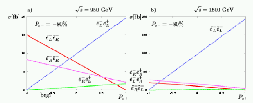
Figure 5.17: Test of selectron quantum numbers in $e^{+}e^{-}\to\tilde{e}_{\rm L,R}^{+}\tilde{e}_{\rm L,R}^{-}$ with fixed electron polarization $P(e^{-})$ = –80% and variable positron polarization $P(e^{+})$. The masses are $m_{\tilde{e}_{\rm L}}$ = 448 GeV, $m_{\tilde{e}_{\rm R}}$ = 417 GeV and a) at $\sqrt{s}$ = 950 GeV both the pairs $\tilde{e}_{\rm L}^{-}\tilde{e}_{\rm L}^{+}$ and $\tilde{e}_{\rm L}^{-}\tilde{e}_{\rm R}^{+}$ have comparable cross sections for unpolarized beams. For $P(e^{+})$ = –40% ($P(e^{+})$ = –60%) the $t$–channel pair $\tilde{e}_{\rm L}^{-}\tilde{e}_{\rm R}^{+}$ dominates by a factor of about 1.5 (about 2). b) At $\sqrt{s}$ = 1500 GeV, the pair $\tilde{e}_{\rm L}^{-}\tilde{e}_{\rm L}^{+}$ dominates kinematically and the $t$-channel process can not be separated.

5.6.2 Gaugino Couplings

At a LC, the parameters of the neutralino/chargino sector and their phases, $M_{1}$, $\Phi_{1}$, $M_{2}$, $\mu$, $\Phi_{\mu}$, and $\tan\beta$ can be determined via the analysis of masses and polarized cross sections without any assumption on the supersymmetry-breaking scheme. Even if only the lighter states $\tilde{\chi}^{0}_{1,2}$ and $\tilde{\chi}^{\pm}_{1}$ are kinematically accessible, a precise determination of these parameters could be made [55]. Once these parameters are known, another important check of fundamental supersymmetric relations could be made with the help of polarized beams: the test whether the SU(2) and U(1) gauge couplings $g$ and $g^{\prime}$ are identical to the gaugino couplings $g_{\tilde{W}}$ and $g_{\tilde{B}}$ from the $\ell\tilde{\ell}\tilde{W}$ and $\ell\tilde{\ell}\tilde{B}$ interactions. The comparison between the polarized cross sections $\sigma_{\rm L}$ and $\sigma_{\rm R}$ for neutralino production with the theoretical prediction for variable ratios $g_{\tilde{W}}/g$ and $g_{\tilde{B}}/g^{\prime}$ provides a precise test of the gaugino couplings at the % level [55, 56].

5.6.3 Distinction between the MSSM and (M+1)SSM

Supersymmetric models with additional chiral or vector superfields give rise to extensions of the gaugino/higgsino sector in general, and additional neutralinos occur. We consider here the (M+1)SSM with one new Higgs singlet, which leads to an extra singlino state. Since the neutralino mass spectra of the lightest four neutralinos in such extended models can be similar to those in the MSSM, a distinction between the models might be difficult. However, the coupling structure is different in the two models. Therefore they could be distinguished via the polarization dependences of the cross sections. In Fig. 5.18 we show the cross section for $e^{+}e^{-}\to\tilde{\chi}^{0}_{1}\tilde{\chi}^{0}_{2}$ for one example in the MSSM and one in the (M+1)SSM [57], where the mass spectra of the light particles in the two models are similar.

Powerful tests for the closure of the system are evaluations of sum rules. The four-state mixing in the MSSM induces sum rules for the couplings that follow from the unitarity of the diagonalization matrices. For asymptotic energies, these sum rules can be transformed directly into sum rules for the associated cross sections [55], and are given in the MSSM by

$$\lim_{s\rightarrow\infty}\,s\,\sum_{i\leq j}^{4}\,\sigma\{ij\}=\frac{\pi\alpha^{2}}{48\,c^{4}_{W}s^{4}_{W}}\left[64s^{4}_{W}-8s^{2}_{W}+5\right]\,.$$ (5.7)

In Fig. 5.19 the exact values for the summed cross sections are shown for one example, normalized to the asymptotic values. The final state $\tilde{\chi}^{0}_{1}\tilde{\chi}^{0}_{1}$ is invisible in $R$-invariant theories, and its detection is difficult. Nevertheless, it can be studied directly by photon tagging in the final state $\gamma\tilde{\chi}^{0}_{1}\tilde{\chi}^{0}_{1}$, which can be observed at the LC. In this example the mass spectra of the light neutralinos in the two models are similar, and the asymptotic cross-section value is not affected by the additional singlet of the (M+1)SSM. However, as can be seen in Fig. 5.19, because of the incompleteness of these states below the thresholds for producing the heavy neutralino, the value measurable in the (M+1)SSM differs significantly from the corresponding sum rule of the MSSM. Therefore, even if the extended neutralino states are very heavy, the study of sum rules can shed light on the underlying structure of the supersymmetric model. In this context, beam polarization is important to enhance the rates of even those pairs that have extremely small cross sections.

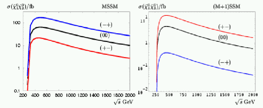
Figure 5.18: Cross sections for the process $\sigma(e^{+}e^{-}\to\tilde{\chi}^{0}_{1}\tilde{\chi}^{0}_{2})$ with polarized beams $(P_{e^{-}}=\pm$ 80%, $P_{e^{+}}=\mp$ 60%) for an example in the MSSM and the (M+1)SSM, where the mass spectra of the light neutralinos are similar [57].

Figure 5.19: The energy dependence of the sum of all the neutralino–pair-production cross sections normalized to the asymptotic form of the summed cross section. The solid line represents the exact sum in the MSSM and the dashed line the sum of the cross sections for the first four neutralino states for a specific parameter set of the (M+1)SSM [55].

5.6.4 Determination of $\tan\beta$ and Trilinear Couplings

Several studies have been made of how $\tan\beta$ can be measured in the Higgs sector via rates, widths and branching ratios [58]. However, if $\tan\beta>$ 10, its precise determination will be difficult. It was shown in Ref. [48, 59] that in this case the $\tau$ and $t$ polarizations are suitable observables for determining $\tan\beta$. The procedure is as follows: one studies the rates for producing the lighter sparticle pairs $e^{+}e^{-}\to\tilde{\tau}_{1}\tilde{\tau}_{1}$ or $\tilde{t}_{1}\tilde{t}_{1}$, and measures the mixing angle of the system by analysing polarized rates, as already worked out in earlier studies [60]. The masses as well as the mixing angle can be measured with precisions at the per cent level. Ambiguities can be resolved, e.g. via measurements of the cross sections with another configuration of the beam polarization [48, 59]. Determining the polarization of the final decay fermions, the $\tau$ or $t$ polarization, while taking into account the complete neutralino and chargino mixing, leads to a determination of $\tan\beta$ with an accuracy of 10% even at high $\tan\beta$. In this context, the measurement of the $t$ polarization from $\tilde{b}_{1}\to t\tilde{\chi}^{\pm}$ decays could be very tricky, since the reconstruction of the system is difficult because of the missing transverse energy. However, analysing the distributions of the quark jets in the hadronic top decays $t\to b+c\bar{s}$ could lead to a very precise measurement of the top polarization [48, 59] as seen in Fig. 5.20.

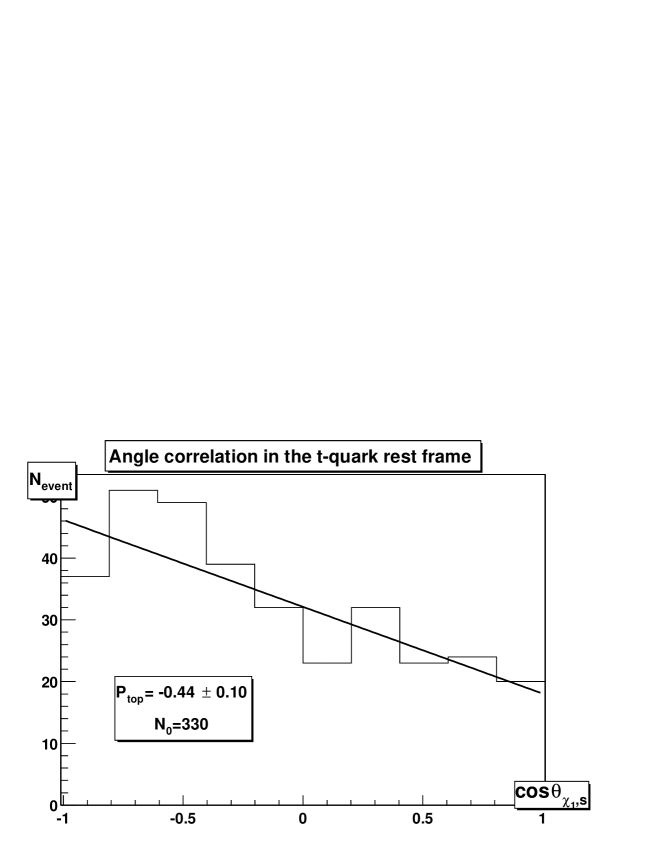
Figure 5.20: Angular distribution in $\cos\theta^{*}_{s}$, the angle between the $\tilde{b}_{1}$ and $\bar{s}$ partons in the top rest frame of $t\to b\,c\bar{s}$ decays from $e^{+}_{L}e^{-}_{R}\to\tilde{b}_{1}\tilde{b}_{1}\to t\tilde{\chi}_{1}^{\pm}+\tilde{b}_{1}$ production at $\sqrt{s}$ = 1.9 TeV. The line represents a fit to a top polarization of $P_{t}$ = – 0.44 $\pm$ 0.10 [48, 59].

If the heavier states $\tilde{\tau}_{2}$, $\tilde{b}_{2}$ or $\tilde{t}_{2}$ are also accessible, one can even go a step further, and determine the trilinear couplings $A_{f}$. If $\tilde{t}_{2}$ and $\tilde{b}_{2}$ can be measured at the per cent level, $A_{t}$ and $A_{b}$ may be extracted with 30–50% precision [21, 59]. Because of the small $\tau$ mass, one cannot expect to determine the parameter $A_{\tau}$ with very high precision.

5.7 Measuring Neutrino Mixing Angles at CLIC

Recent neutrino experiments [61, 62, 63] clearly show that neutrinos are massive particles and that they mix. A possible way to account for the observed neutrino data in supersymmetric theories is to break lepton number, either spontaneously or explicitly, and thus R-parity. The simplest realization of this idea is to add bilinear terms to the superpotential $W$:

$$W=W_{\rm MSSM}+\epsilon_{i}\hat{L}_{i}\hat{H}_{u}\,.$$ (5.8)

For consistency one also has to add the corresponding bilinear terms to soft SUSY-breaking, which induce small vacuum expectation values (vevs) for the sneutrinos. These vevs induce a mixing between neutrinos and neutralinos, giving mass to one neutrino. The second neutrino mass is induced by loop effects (see Ref. [64] and references therein). The same parameters that induce neutrino masses and mixings are also responsible for the decay of the lightest supersymmetric particle (LSP). This implies that there are correlations between neutrino physics and LSP decays [65, 66, 67].

As a specific example we present the relationship between the atmospheric neutrino mixing angle and the decays of a neutralino into semileptonic final states $l_{i}q^{\prime}\bar{q}$ ($l_{i}=e,\mu,\tau$). There are several more examples, which are discussed in Ref. [66]. In the model specified by Eq. (5.8) the atmospheric mixing angle is given by

$$\tan\theta_{\rm atm}=\frac{\Lambda_{2}}{\Lambda_{3}}$$ (5.9)

$$\Lambda_{i}=\epsilon_{i}v_{d}+\mu v_{i}\,,$$ (5.10)

where $v_{i}$ are the sneutrino vevs and $v_{d}$ is the vev of $H^{0}_{1}$. It turns out that the dominant part of the $\tilde{\chi}^{0}_{1}$-$W$-$l_{i}$ coupling $O^{L}_{i}$ is given by

$$O^{L}_{i}=\Lambda_{i}f(M_{1},M_{2},\mu,\tan\beta,v_{d},v_{u})\,,$$ (5.11)

where the exact form of $f$ can be found in Eq. (20) of Ref. [66]. The important point is, that $f$ depends only on MSSM parameters and not on the R-parity-violating parameters. Putting everything together one finds:

$$\tan^{2}\theta^{2}_{\rm atm}=\left|\frac{\Lambda_{2}}{\Lambda_{3}}\right|^{2}\simeq\frac{BR(\tilde{\chi}^{0}_{1}\to\mu^{\pm}W^{\mp})}{BR(\tilde{\chi}^{0}_{1}\to\tau^{\pm}W^{\mp})}\simeq\frac{BR(\tilde{\chi}^{0}_{1}\to\mu^{\pm}\bar{q}q^{\prime})}{BR(\tilde{\chi}^{0}_{1}\to\tau^{\pm}\bar{q}q^{\prime})}\,.$$ (5.12)

The restriction to the hadronic final states of the $W$ is necessary for the identification of the lepton flavour. Depending on the specific parameters, one gets additional small contributions due to three-body decays of intermediate sleptons and squarks. Note that Eq. (5.12) is a prediction of the bilinear model independent of the R-parity-conserving parameters. It has been shown that under favourable conditions the LHC can measure the ratio of branching ratios in Eq. (5.12) with an accuracy of about 3% [68].

In this note we study an example of such a correlation in a scenario where the lightest neutralino is rather heavy and where it is most likely that the LHC will have difficulties to measure the branching ratios accurately. For the numerical example, we take point H as reference, which is characterized by $M_{1/2}$ = 1.5 TeV, $M_{0}$ = 419 GeV, $A_{0}$ = 0, $\tan\beta$ = 20 and a positive sign of $\mu$. We vary randomly the R-parity-conserving parameters around this point so that the masses of the supersymmetric particles vary within 10% for the particles that can be observed at a 5 TeV collider. For the remaining particles we set a lower cut of 2.5 TeV on the masses. To these sets of parameters we add the R-parity-breaking parameters such that the correct differences between the squared neutrino masses and the correct mixing angles are obtained within the experimental allowed range: 1.2 $\times$ 10^-3 eV${}^{2}<\Delta m^{2}_{\rm atm}<$ 4.8 $\times$ 10^-3 eV², 5.1 $\times$ 10^-5 eV${}^{2}<\Delta m^{2}_{\rm sol}<$ 1.9 $\times$ 10^-4 eV², 0.29 $<\sin^{2}\theta_{\rm atm}<$ 0.86, $\sin^{2}\theta_{13}<$ 0.05. For illustrative purpose only we allow a range for $\sin^{2}\theta_{\rm atm}$ wider than the experimentally allowed one: 0.3 $<\sin^{2}\theta_{\rm atm}<$ 0.7. The main LSP decay modes are: BR$(\tilde{\chi}^{0}_{1}\to h^{0}\sum_{i~{}=~{}1,3}\nu_{i})\simeq$ 50%, BR$(\tilde{\chi}^{0}_{1}\to W^{\pm}e^{\mp}+W^{\pm}\mu^{\mp}+W^{\pm}\tau^{\mp})\simeq$ 30%, BR$(\tilde{\chi}^{0}_{1}\to Z^{0}\sum_{i~{}=~{}1,3}\nu_{i})\simeq 20$%. In addition there are three-body decay modes mainly mediated by virtual sleptons whose sum of the branching ratios is about 1–2%.

In Fig. 5.21 we show the correlation between $\tan^{2}\theta_{\rm atm}$ and $BR(\tilde{\chi}^{0}_{1}\to\mu^{\pm}\bar{q}q^{\prime})/BR(\tilde{\chi}^{0}_{1}\to\tau^{\pm}\bar{q}q^{\prime})$. Note that the width of the band is due to the variation of the parameters as discussed above. It becomes by a factor of 4–5 smaller if the SUSY masses can be measured with an accuracy of 2% instead of the assumed 10%. Figure 5.21 clearly shows that these decay modes can be used to relate observables measured at CLIC to those measured at neutrino experiments. Moreover, they allow for a consistency test of the theory. Note that R-parity-violating decay modes into gauge bosons (Higgs bosons) and leptons are forbidden in R-parity-violating models where only trilinear R-parity-breaking couplings exist. Therefore, the observation of such decays give a clear proof that bilinear R-parity-breaking is realized in nature.

Figure 5.21: Correlation between atmospheric neutrino mixing angle and semileptonic branching ratios of the lightest neutralino.

In summary, models where R-parity is broken by bilinear terms can explain recent neutrino data and predict at the same time certain decay properties of the lightest supersymmetric particle. CLIC is particularly suited to explore the resulting correlations between neutrino mixing angles and ratios of LSP branching ratios in scenarios where the LSP is rather heavy.

5.8 Summary

The CLIC multi-TeV linear $e^{+}e^{-}$ collider has important potential for supplementing the information on supersymmetry that might be provided by previous colliders such as the LHC and a TeV-class linear collider, as we have illustrated within the CMSSM. The CMSSM parameter space is restricted by experimental constraints from LEP and elsewhere, and by cosmology. If sparticle masses are in the lower part of the range still allowed by these constraints, much of the supersymmetric spectrum will have been discovered by the LHC and/or by a TeV-class linear collider, which would also be able to make some precision measurements. In this case, CLIC would be invaluable for extending precision measurements to squarks and heavier neutralinos and charginos, in particular. On the other hand, if sparticle masses are in the upper part of the allowed range, CLIC might be the first accelerator to produce many of the SUSY particles.

Using benchmark CMSSM points as examples, we have demonstrated that CLIC would be able to make detailed measurements of sparticle masses and mixing angles. These would enable accurate tests of unification hypotheses for mechanisms of supersymmetry breaking to be made. Electron and positron beam polarization would be a useful tool for disentangling sparticle properties, and the $\gamma\gamma$ option would be especially interesting for gluino production, in particular. Although most of this discussion referred to the CMSSM, we have also shown that CLIC has important capabilities for distinguishing this from more complicated supersymmetric models, and for exploring scenarios in which R parity is violated.

We conclude that CLIC will be an invaluable tool for exploring supersymmetry, even if it has been discovered previously at the LHC and explored at a TeV-class linear collider.

Chapter 6 PROBING NEW THEORIES

The LHC is expected to probe directly possible new physics (NP) beyond the Standard Model (SM) up to a scale of a few TeV. While its data should provide answers to several of the major open questions in the present picture of elementary particle physics, it is important to start examining how this sensitivity can be further extended at a next generation of colliders. Today we have a number of indications that NP could be of supersymmetric nature. If this is the case, the LHC will have a variety of signals to discover these new particles, and a linear collider will be required to complement the probe of the supersymmetric spectrum with detailed measurements, as discussed in the previous chapter. However, beyond supersymmetry, there is a wide range of other scenarios invoking new phenomena at, and beyond, the TeV scale. They are aimed at explaining the origin of electroweak symmetry breaking, if there is no light elementary Higgs boson, at stabilizing the SM, if supersymmetry is not realized in nature, or at embedding the SM in a theory of grand unification.

6.1 Extra Dimensions

In the last few years there has been considerable interest in the possibility that new spatial dimensions can be observed at high-energy colliders. One interesting theoretical option is that only gravity propagates in the extra dimensions, whilst gauge and matter fields are confined on a three-dimensional brane [2, 3]. This hypothesis is motivated by the hierarchy problem and naturally realized in string theory. Two different kinds of scenarios have been proposed: those in which the space metrics are factorizable [2] and those in which they are non-factorizable [3]. Their relative phenomenological consequences are quite distinct. When discussing the experimental signals of these models, one should bear in mind that the theory is non-renormalizable, with an unknown ultraviolet completion. It is then necessary to distinguish various kinematical regimes, which can be tackled with different theoretical tools.

We first consider the cisplanckian region, in which the centre-of-mass energy of the collision is much smaller than the fundamental quantum-gravity scale $M_{D}$. We can then describe graviton production using an effective theory obtained by linearizing the Einstein action. In the case of factorizable extra dimensions, we obtain a nearly-continuous spectrum of Kaluza–Klein (KK) graviton excitations, which interact very weakly and give rise to experimental missing-energy signatures.

In the case of non-factorizable metrics, the graviton KK excitations have mass gaps of the order of the fundamental scale $M_{D}$ and they have a sizeable interaction with ordinary matter, leading to characteristic resonant production at high-energy collisions. A study of the predictions for CLIC and the comparison with the LHC reach is presented in Section 1.2.

The effective theory, valid at energies below $M_{D}$, also contains the most general set of gauge-invariant higher-dimensional operators. The coefficients of these operators cannot be computed without knowledge of the short-distance theory. Therefore, a general experimental study of contact interactions will be very useful to gain information about the underlying theory. One can perform a more restrictive (but more predictive) analysis by considering only those operators generated by graviton exchange. At tree level, a single dimension-8 operator is generated. This operator contributes to a variety of processes at CLIC. The most interesting is probably $e^{+}e^{-}\to\gamma\gamma$, since no other local operator of lower dimension can generate this process. Therefore, the study of diphoton final states can be of particular importance in probing new gravitational effects. The exchange of gravitons at the loop level generates a single dimension-6 operator, which is the product of two flavour-universal axial currents. In this case, the relevant final state is dilepton or dijet. We do not pursue here an analysis of these processes, but we refer the reader to the later section on contact interactions.

At centre-of-mass energies of the order of $M_{D}$, we are entering the Planckian region, where the effective theory approach discussed above is no longer valid. This is the most interesting region from the experimental point of view, since new phenomena related to quantum gravity and string theory will fully manifest themselves. However, it is also the most difficult region to tackle theoretically, in the absence of a complete description of the short-distance behaviour of gravity. It is however easy to predict that, in case of a discovery at the LHC, the rôle of a multi-TeV linear collider will be crucial to disentangle the new physics signals, leading to new understanding of the underlying theory.

In the transplanckian region, where $\sqrt{s}\gg M_{D}$, we can give a reliable description of the scattering process (at least under certain kinematical conditions), since semiclassical physics give the dominant effects. At impact parameters larger than the Schwarzschild radius, gravitational elastic scattering is computable in the eikonal approximation. This gives a prediction for Bhabha scattering at small angles which can be compared with observations at CLIC. When the impact parameter is of the order of the Schwarzschild radius or smaller, strong classical-gravity effects complicate the theoretical description, but there are plausible arguments that suggest that black holes are formed. If this is the case, any purely short-distance interactions from quantum gravity will be masked by the black hole, as the collision energy is increased. We also briefly discuss some of the implications of transplanckian physics at CLIC.

So far we have considered the case in which gauge and matter fields are strictly four-dimensional. It is not implausible that, within the scenarios considered above, also SM fields have extra-dimensional excitations, although different in nature from those of the gravitons. We consider such possibility in Section 1.4, where we describe the present bounds on KK excitations of SM fields and future prospects for discovery at CLIC. To emphasize the importance of the complementarity rôle of a multi-TeV linear collider with respect to the LHC, we also discuss in Section 1.4 how studies at CLIC can distinguish between the surprisingly similar collider signals of KK excitations of SM particles from those of a supersymmetric model with a nearly degenerate superpartner spectrum.

6.1.1 ADD Type of Extra Dimensions

The first model we consider is that of Arkani-Hamed, Dimopoulos and Dvali (ADD) [2]; we limit our discussion to the case of graviton tower exchange in $e^{+}e^{-}\to f\bar{f}$. The effect of summing the KK gravitons is to produce a set of effective dimension-8 operators of the form $\sim\lambda T^{\mu\nu}T_{\mu\nu}/M_{s}^{4}$, where $T_{\mu\nu}$ is the stress-energy tensor of the SM matter exchanging the tower[4]. This approximation only applies in the limit that the centre-of-mass energy of the collision process lies sufficiently below the cut-off scale $M_{s}$, which is of the order of the size of the Planck scale in the extra-dimensional space. In the convention used by Hewett [4] and adopted here, the contribution of the spin-2 exchanges can be universally expressed in terms of the scale $M_{s}$ and a sign $\lambda$. Current experimental constraints from LEP and the Tevatron[5] tell us that $M_{s}\geq 1$ TeV for either sign of $\lambda$; values of $M_{s}$ as large as the low 10’s of TeV may be contemplated in this scenario.

In the case of $e^{+}e^{-}\to f\bar{f}$, the addition of KK tower exchange leads to significant deviations in differential cross Sections and polarization asymmetries from their SM values, which are strongly dependent on both the sign of $\lambda$ and the ratio $s/M_{s}^{2}$. Such shifts are observable in final states of all flavours. In addition, the shape of these deviations from the SM with varying energy and scattering angle, as shown by Hewett [4], tells us that the underlying physics arises from dimension-8 operators and not, for example, $Z^{\prime}$ exchange. Figure 6.1 shows an example of how such deviations from the SM might appear at a 5-TeV CLIC in the case that $M_{s}$ = 15 TeV for either sign of $\lambda$.

     

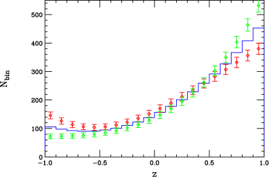
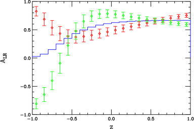
Figure 6.1: Deviations in the cross section for $\mu$ pairs (left) and $A_{\rm LR}$ for $b$ quarks (right) at $\sqrt{s}$ = 5 TeV for $M_{s}$ = 15 TeV in the ADD model for an integrated luminosity of 1 ${\rm ab}^{-1}$. The SM is represented by the histogram while the red and green data points show the ADD predictions with $\lambda=\pm$ 1. In both plots $z=\cos\theta$.

The indirect search reach for the scale $M_{s}$ can be obtained by combining the data for several of the fermion final states ($\mu,\tau,c,b,t$, etc.) in a single overall fit. The result of this analysis for CLIC is the $\lambda$-independent bound shown in Fig. 6.2 as a function of the integrated luminosity for $\sqrt{s}$ = 3 or 5 TeV. For an integrated luminosity of 1 ${\rm ab}^{-1}$ we see that the reach is $M_{s}\simeq 6\sqrt{s}$, which is consistent with analyses at lower-energy machines [4].

     

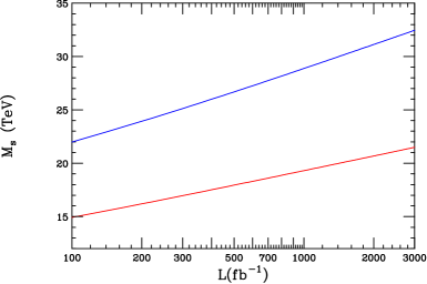
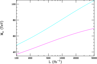
Figure 6.2: (Left) Search reach for the ADD model scale $M_{s}$ at CLIC as a function of the integrated luminosity from the set of processes $e^{+}e^{-}\to f\bar{f}$, assuming $\sqrt{s}$ = 3 (bottom) or 5 (top) TeV. Here $f=\mu,\tau,b,c$, $t$, etc. (Right) Corresponding reach for the compactification scale of the KK gauge bosons in the case of one extra dimension and all fermions localized at the same orbifold fixed point.

Scenarios with large extra dimensions have been studied for TeV-class linear colliders, e.g. TESLA [6], and are searched for typically in the channel $e^{+}e^{-}\rightarrow\gamma+G$. One of the acclaimed advantages of a LC with respect to the LHC is that, by measuring the $\gamma G$ cross section at different centre-of-mass energies, one can disentangle the Planck scale and the number of extra dimensions $\delta$ simultaneously, as is shown for CLIC in Fig. 6.3 by the solid lines. The cross sections are calculated for cuts similar to those in [6]: $\sin\theta_{\gamma}>$ 0.1, $p^{\gamma}_{t}>$ 0.06 $E_{\rm beam}$ and $x_{\gamma}<$ 0.65. The cross sections are normalized in such a way that for each value of $\delta$, the scale $M_{D}$ is chosen to give the same cross section at 500 GeV.

These predictions assume, however, that lower-dimensional physics is attached to rigid branes. Allowing for flexible branes instead [7] introduces a new dependence on a parameter $\Delta$, the softening scale, which is related to the brane tension. The dashed lines in Fig. 6.3 show the effect of $\Delta$ for values of 4 TeV and 1 TeV, respectively.

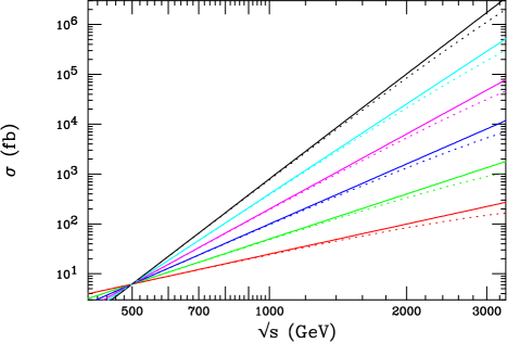
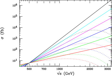
Figure 6.3: The cross section for $e^{+}e^{-}\rightarrow G\gamma$ with cuts as described in the text, for rigid (solid lines) and soft (dashed lines) branes. The different curves correspond, from bottom to top, to different numbers of extra dimensions $\delta$ = 2, 3, 4, 5, 6 and 7. Left, for $\Delta$ = 4 TeV, right for $\Delta$ = 1 TeV.

For a brane tension of 4 TeV, the effect on the cross section is rather small. A collider in the range of 0.5–1 TeV would not be sensitive to the effect and thus $M_{D}$ and $\delta$ can still be disentangled. However, at CLIC the cross sections are 30–40% lower than expected, allowing one to observe the softness of the brane. For a brane of 1 TeV tension the effect is more spectacular. For the example given here, a lower-energy LC would get fooled when measuring cross sections only at 0.5 TeV and 1 TeV, and extract wrong values of $\delta$ and $M_{D}$. Extending the range in the multi-TeV region will again allow this effect to be observed in its full drama. The cross section of the background channel $e^{+}e^{-}\rightarrow e^{+}e^{-}\gamma$ with the cuts as listed above is 16 fb at 3 TeV, which sets the scale for the detectability of a signal: for $\delta$ = 2 or 3 the signal event rate at 3 TeV gets too small for such a soft brane scenario.

6.1.2 Graviton Production at CLIC: Randall–Sundrum Model

In the extra-dimension scenario proposed by Randall and Sundrum (RS) [3] the hierarchy between the Planck and the electroweak scale is generated by an exponential function called the ‘warp factor’. This model predicts KK graviton resonances with weak-scale masses and strong couplings to matter. Hence the production of TeV-scale graviton resonances is expected in two-fermion channels [8]. In its simplest version, with two branes and one extra dimension, and where all of the SM fields remain on the brane, the model has two fundamental parameters: the mass of the first KK state $m_{1}$, and the parameter $c=k/M_{\overline{Pl}}$, where $k$ is related to the curvature of the 5D space and $M_{\overline{\rm Pl}}$ is the 4D effective Planck scale. The parameter $c$ controls the effective coupling strength of the graviton and thus the width of the resonances, and should be less than 1 but yet not too far away from unity.

The resulting spectrum for $e^{+}e^{-}\rightarrow\mu^{+}\mu^{-}$ is shown in Fig. 6.4. The cross sections are huge and the signal cannot be missed at a LC with sufficient centre-of-mass energy. If such resonances are observed — perhaps first by the LHC in the range of a few TeV — it will be important to establish the nature of these newly produced particles, i.e. to measure their properties (mass, width and branching ratios) and quantum numbers (spin). Note that the mass $m_{1}$ of the first resonance determines the resonance pattern: the masses of all higher-mass resonances are then fixed.

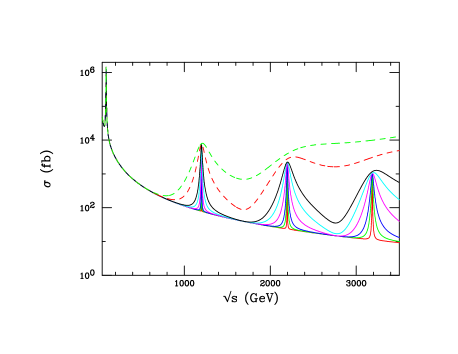
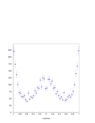
Figure 6.4: Left: KK graviton excitations in the RS model produced in the process $e^{+}e^{-}\to\mu^{+}\mu^{-}$. From the most narrow to widest resonances, the curves are for 0.01 $<c<$ 0.2. Right: Decay-angle distribution of the muons from $G_{3}$ (3200 GeV) $\to\mu\mu$.

The signal for one KK resonance ($G_{1}$) is implemented in PYTHIA 6.158 [9] via process 41. For the study, PYTHIA has been extended to include two more resonances ($G_{2},G_{3}$, corresponding to processes 42 and 43) to allow a check on the measurability of the graviton self-coupling. The decay branching ratios of these resonances were modified according to [8, 10]. In particular, the gravitons can decay into two photons in about 4% of the cases, a signature that would distinguish them from, for example, new heavy $Z^{\prime}$ states [11].

The resonance spectrum was chosen such that the first resonance $G_{1}$ has a mass around 1.2 TeV, just outside the reach of a TeV-class LC, and consequently the mass of the third resonance $G_{3}$ will be around 3.2 TeV, as shown in Fig. 6.4. The $\sqrt{s}$ energy for the $e^{+}e^{-}$ collisions of CLIC was taken to be 3.2 TeV in this study. Mainly the muon and photon decay modes of the graviton have been studied. The events used to reconstruct the $G_{3}$ resonance signal were selected via either two muons or two $\gamma$’s with $E>$ 1200 GeV and $|\cos\theta|<$ 0.97. The background from overlaid two-photon events — on average four events per bunch crossing — is typically important only for angles below 120 mrad, i.e. outside the signal search region considered.

First we study the precision with which one can measure the shape, i.e. the $c$ and $M$ parameters, of the observed new resonance. A scan similar to that of the $Z$ at LEP was made for an integrated luminosity of 1 ab^-1. The precision with which the cross sections are measured allows one to determine $c$ to 0.2% and $M$ to better than 0.1%.

Next we determine some key properties of the new resonance: the spin and the branching ratios. The graviton is a spin-2 object, and Fig. 6.4 shows the decay angle of the fermions $G\rightarrow\mu\mu$ for the $G_{3}$ graviton, obtained using PYTHIA/SIMDET for 1 ab^-1 of data, including the CLIC machine background. The typical spin-2 structure of the decay angle of the resonance is clearly visible.

For gravitons as proposed in [8, 10] one expects $BR(G\rightarrow\gamma\gamma)/BR(G\rightarrow\mu\mu)$ = 2. With the present SIMDET simulation we get efficiencies in the mass peak ($\pm~{}200$  GeV) of 84% and 97% for detecting the muon and photon decay modes, respectively. With cross sections of O(1 pb), $\sigma_{\gamma\gamma}$ and $\sigma_{\mu\mu}$ can be determined to better than a per cent. Hence the ratio $BR(G\rightarrow\gamma\gamma)/BR(G\rightarrow\mu\mu)$ can be determined to an accuracy of 1% or better.

Finally, if the centre-of-mass energy of the collider is large enough to produce the first three resonance states, one has the intriguing possibility to measure the graviton self-coupling via the $G_{3}\rightarrow G_{1}G_{1}$ decay [10]. The dominant decay mode will be $G_{1}\rightarrow gg$ or $q\bar{q}$ giving a two-jet topology. Figure 6.5 shows the resulting spectacular event signature of four jets of about 500 GeV each in the detector (no background is overlaid). These jets can be used to reconstruct $G_{1}$. Figure 6.5 shows the reconstructed $G_{1}$ invariant mass. The histogram does not include the background, while the dots include 10 bunch crossings of background overlaid on the signal events. Hence the mass of $G_{1}$ can be well reconstructed and is not significantly distorted by the $\gamma\gamma$ background.

          

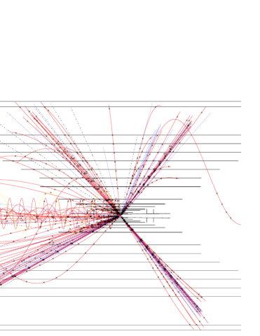
Figure 6.5: Left: Event in a CLIC central detector with the decay $G_{3}\rightarrow G_{1}G_{1}\rightarrow$ four jets. Right: Invariant jet–jet mass of $G_{1}$(1200 GeV) produced in $G_{3}\rightarrow G_{1}G_{1}$ and $G_{1}\rightarrow$ two jets.

In summary, a multi-TeV collider such as CLIC will allow a precise determination of the shape and mass of the new resonance(s), and of its spin. In particular, for the RS model it was shown that the key discriminating properties of these resonances can be reconstructed, and the underlying model parameters can be determined precisely.

6.1.3 Transplanckian Scattering

Elastic collisions in the transplanckian region, where the centre-of-mass energy $\sqrt{s}$ is much larger than the fundamental gravity mass scale $M_{D}$, can be described by linearized general relativity and known quantum-mechanical effects, as long as the momentum transfer in the process is sufficiently small. Therefore, the interesting observable at CLIC is Bhabha scattering at small deflection angle. The relevant cross section can be computed using the eikonal approximation, in the kinematical regime in which the impact parameter is smaller than the Schwartzschild radius

$$R_{S}=\frac{2\sqrt{\pi}}{M_{D}}\left[\frac{\Gamma\left(\frac{\delta+3}{2}\right)}{2\pi^{2}(\delta+2)}\frac{\sqrt{s}}{M_{D}}\right]^{\frac{1}{\delta+1}}.$$

At small momentum transfer $t$, the gravitational-scattering differential cross section is

$$\frac{d\sigma}{dt}=C_{\delta}\frac{\sigma_{BH}}{s}\left(\frac{s}{M_{D}^{2}}\right)^{\frac{(\delta+2)^{2}}{\delta(\delta+1)}},~{}~{}~{}~{}\sigma_{BH}=\pi R_{S}^{2}\,,$$

where $C_{\delta}$ is a $\delta$-dependent coefficient. With large gravity-induced cross sections ($\sim$ 10²–10³ pb) for all $M_{D}/\sqrt{s}\ll$ 1, combined with relatively low background, CLIC could certainly provide very important tests of extra-dimensional theories. The maximum values of $M_{D}$ that can be studied at CLIC in the transplanckian gravitational scattering are uniquely determined by the condition for validity of the eikonal approximation ($\sqrt{s}\gg M_{D}$). Therefore very high energies should be achieved to compete with the LHC. However, the cleaner $e^{+}e^{-}$ environment offers several advantages for precision tests and parameter determinations.

For our study, we consider centre-of-mass energies as high as 10 TeV, but it is not difficult to rescale our results to different values of $\sqrt{s}$. In Fig. 6.6 we give one example of the signal and background distributions in the scattering angle $\theta$ for $M_{D}$ = 2 TeV. Here $\theta$ is the scattering angle of the electron in the Bhabha process, and $\theta$ = 0 indicates the electron going down the beam pipe undeflected by the collision. Notice that the SM background is completely insignificant as long as we exclude a small region along the beam direction. This allows experimental studies of the cross section in a much more forward region than what is possible at the LHC.

Figure 6.6: Angular distribution of the $e^{+}e^{-}\to e^{+}e^{-}$ signal for $M_{D}$ = 2 TeV and $\sqrt{s}$ = 10 TeV. The solid line is for $\delta$ = 6, the dotted for $\delta$ = 4 and the dashed for $\delta$ = 2. The almost-vertical dash-dotted line at the far left of the figure is the Bhabha scattering rate expected from the Standard Model.

The signal angular distribution is characterized by the peak structure shown in Fig. 6.6, with the first peak approximately given by

$$\theta^{\rm peak}\simeq\left(\frac{a_{\delta}M_{D}}{\sqrt{s}}\right)^{\frac{\delta+2}{\delta}},$$

where $a_{\delta}$ is a numerical coefficient with the values $a_{2,3,4,5,6}$ = 0.9, 1.2, 1.1, 1.1, 1.0. The $\delta$ = 6 line (solid line) in Fig. 6.6 is the most telling line, since a careful measurement of the ups and downs of $d\sigma/d\theta$ would be hard to reproduce in another framework. Given the good energy and angular resolutions that can be achieved at a linear collider, CLIC could perform a much more precise study of the peak structure than what is feasible at the LHC.

Another advantage of CLIC is that, unlike a $pp$ collider, the scattering particles are distinguishable. This means that the calculable limit of $t\to$ 0 (small-angle scattering) is unambiguously identifiable. On the other hand, in the $pp$ collider case, the case of partons glancing off each other at $\hat{t}\to$ 0 is not distinguishable from partons bouncing backwards at large momentum transfer $\hat{t}\to-\hat{s}$. It is plausible that these non-calculable large momentum transfer contributions are negligible, but CLIC can test that assertion.

At large scattering angle, when $t$ approaches $s$, the eikonal description breaks down, and non-linear gravitational effects cannot be neglected. Although a complete calculation has not been performed, it is plausible to assume that black holes are formed. If the fundamental scale $M_{D}$ lies in the TeV range, the cross section is expected to be very large, as in the case of the elastic scattering discussed above: $\sigma\simeq\sigma_{\rm BH}\sim$ O(100) pb (TeV$/M_{D})^{2}$. The lifetime of such a black hole is of order $\sim$ 10^-25–10^-27 s, and hence the black hole will evaporate before it could possibly ‘attack’ any detector material, certainly causing no safety concern.

In a first approximation, such a machine produces black holes of a fixed mass, equal to the energy of the machine. The total cross section of such a black hole produced at a 3 TeV and a 5 TeV machine, as a function of $m_{p}$ and $n$, is shown in Fig 6.7a and Fig. 6.7f, respectively. For more elaborated studies of black-hole production at electron colliders, one should take into account the machine luminosity spectrum as discussed in Section 6. Using the beamsstrahlung spectra for a 3- or 5-TeV CLIC machine, we show the differential cross section $d\sigma/dM_{\rm BH}$ for black hole production at a 3- and 5-TeV CLIC machine in Figs. 6.7e and Fig. 6.7j, respectively.

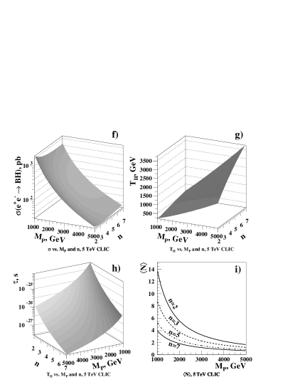
Figure 6.7: Black hole properties at CLIC. Plots a)–d) and f)–i) correspond to the properties (production cross section, temperature, lifetime, and average decay multiplicity) of a fixed-mass 3-TeV and 5-TeV black hole produced at a 3-TeV or 5-TeV machine, respectively. Plots e), j) show the differential cross section of black-hole production for $n$ = 4, as a function of the black-hole mass at a 3-TeV or 5-TeV CLIC $e^{+}e^{-}$ collider, respectively.

Black hole production at CLIC is complementary to the LHC in many ways, as the maximum number of black holes produced at CLIC is found at the highest accessible masses. This gives some advantage, as the stringy effects and the kinematic distortion of the Planck black-body spectrum decrease with the increase of the black-hole mass. This can be used to extract the dimensionality of the extra space, by observing the relationship between the black-hole horizon temperature ($T_{\rm H}$) vs. the mass of the black hole, as suggested in [12]. This method is less affected at CLIC by unknown stringy and kinematic effects. Preliminary studies show that the statistical sensitivity to the number of extra dimensions and the value of the fundamental Planck scale at CLIC is similar to that at the LHC.

The decay of a black hole can be very complex and involves several stages [13]. If the dominant mode is Hawking radiation, then all particles (quarks, gluons, gauge bosons, leptons) are expected to be produced democratically, with, for instance, a ratio 1/5 between leptonic and hadronic activity. The multiplicity is expected to be large. The production and decay processes have been included in the PYTHIA generator [14]. Figure 6.8 shows two black-hole events produced in a detector at CLIC, leading to spectacular multijet and lepton/photon signals. As an example, Fig. 6.9 shows the sphericity of the events measured after detector simulation and addition of 5 bunch crossings of $\gamma\gamma$ background for black holes and conventional annihilation events.

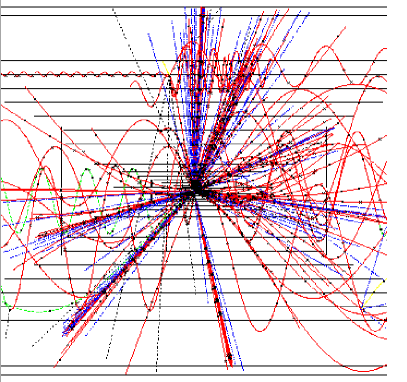
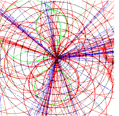
Figure 6.8: Black hole production in a CLIC detector

If this scenario is realized in nature, black holes will be produced at high rates at the LHC. CLIC can be very instrumental in providing precise measurements. For example, it may be possible to test Hawking radiation or get information on the number of underlying extra dimensions.

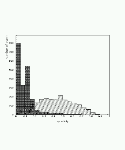
Figure 6.9: Black hole production in a CLIC detector: Sphericity distribution for 2- and 4-fermion events (full histogram) and black holes (hatched histogram)

6.1.4 Kaluza–Klein Excitations in Theories with Extra Dimensions

Another class of models that leads to a resonance structure in the energy dependence of the two-fermion cross section has a TeV-scale extra dimension [15]. In the simplest versions of these theories, only the SM gauge fields are in the bulk, whereas the fermions remain at one of the two orbifold fixed points; Higgs fields may lie at the fixed points or propagate in the bulk. In such a model, to a good approximation, the masses of the KK tower states are given by $M_{n}=nM$, where $M=R^{-1}$ is the compactification scale and $R$ is the compactification radius.

6.1.4.1 Kaluza–Klein excitations in two-fermion processes

The masses and couplings of the KK excitations are compactification-scheme-dependent and lead to a rather complex KK spectrum. Examples of models with one or more extra dimensions, assuming $M$ = 4 TeV, are shown in Fig. 6.10. The positions of the peaks and dips and their corresponding cross sections and widths can be used to identify uniquely the extra-dimensional model. As an example, one of these models was taken and the production cross section was folded with the CLIC luminosity spectrum. The result is shown in Fig. 6.10 for the dip position, since the peaks are likely to be beyond the reach of a 3-TeV collider. The structure of the dip is largely preserved. It is smeared and somewhat systematically shifted, but also here the CLIC data will be sensitive to the model parameters, and will allow one to disentangle different scenarios.

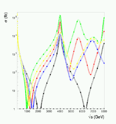
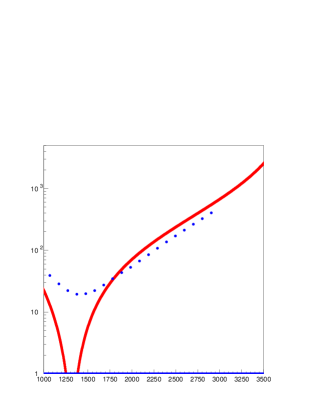
Figure 6.10: Left: The cross section $\sigma_{\mu\mu}$ for different models for TeV-scale extra dimensions. Right: The cross section $\sigma_{\mu\mu}$ before (solid line) and after (dotted line) smearing by the CLIC luminosity spectrum.

Among the models with extra dimensions, we have studied a 5D extension of the SM with fermions on the $y$ = 0 brane of the $S^{1}/Z_{2}$ orbifold. This predicts KK excitations of the SM gauge bosons with fermion couplings a factor of $\sqrt{2}$ larger than those of the SM [16]. We have considered two Higgs bosons: one on the $y$ = 0 brane and the other propagating in the bulk. Indirect limits from electroweak measurements already exist and are derived by considering the modifications to the electroweak observables at the $Z^{0}$ peak and at low energy [17]. The masses of the lowest-lying KK states are constrained to be rather large, i.e. a few TeV, depending on the value of $\beta$, which is related to the ratio between the vev’s of the two Higgs fields and consequently parametrizes the mixing between the KK excitations and the SM gauge bosons. Bounds can be derived by considering the latest experimental values of the $\epsilon$ parameters coming from the precision measurement data [18]. The 95% C.L. lower bounds on the scale $M$ at fixed $s_{\beta}$, coming from the $\epsilon$ observables, are given by the upper curves in Figs. 6.11. The two curves correspond to $m_{t}$ = 175.3 GeV with $m_{H}$ = 98 GeV and 180 GeV. The curve for $m_{H}$ = 120 GeV is very close to the one for $m_{H}$ = 98 GeV. Bounds can be also obtained from low-energy neutral-current experiments, for example, from the atomic parity-violation (APV) experiments. Nevertheless, they lie significantly below the corresponding high-energy limits, and are shown by the lower curves in Fig. 6.12. Bounds can be derived from cross sections at LEP 2 energies. By combining with the precision data, the 95% C.L. lower limit on $M$ is around 6.8 TeV, while the expected sensitivity at the LHC for 100 fb^-1 is around 13–15 TeV, depending on the assumed systematics [19].

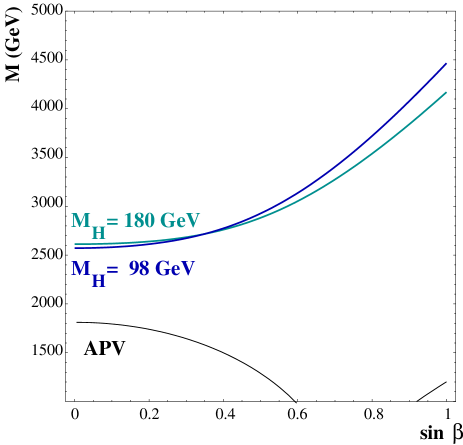
Figure 6.11: 95% C.L. lower bounds on the compactification scale $M$, as functions of $\sin\beta$, from the high-energy precision measurements ($\epsilon$ parameters) and from the APV data. The regions below the lines are excluded.

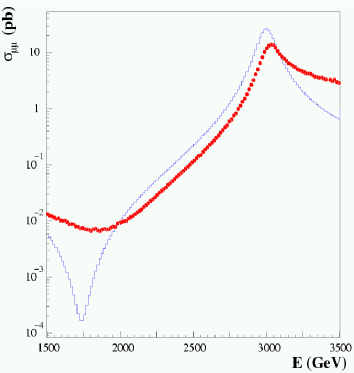
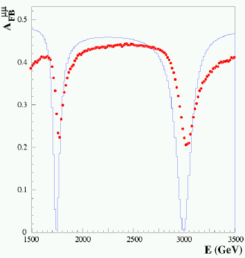
Figure 6.12: $\mu^{+}\mu^{-}$ production cross sections (left) and forward–backward asymmetry (right) in the 5D SM, including the lower KK excitations of the $Z^{0}$ and $\gamma$ with $M_{Z^{(1)}}\sim M_{\gamma^{(1)}}$ = 3 TeV. The continuous lines represent the Born-level expectations, while the dots include the effect of the CLIC luminosity spectrum.

At CLIC, the lowest excitations $Z^{(1)}$ and $\gamma^{(1)}$ could be directly produced [20]. Results for the $\mu^{+}\mu^{-}$ cross sections and forward–backward asymmetries at the Born level and after folding the effects of the CLIC.02 beam spectrum are shown in Fig. 6.12.

Hence, if KK excitations appear in the two-fermion processes, cross Sections in the TeV range, CLIC will be an ideal tool to study in detail the properties of these resonances.

6.1.4.2 Hidden Higgs boson in TeV^-1 type of extra dimensions

In this section the ability of present and future colliders to find the lightest Higgs boson in a model that assumes it has a non-trivial ‘location’ in a 5D space is explored, in the context of TeV-scale extra dimensional models. The currently missing signal is then due to a suppression of the Higgs production cross section at LEP and the Tevatron. The model promises a significant enhancement of the signal at the LHC and possibly at a multi-TeV linear collider (CLIC). We present results for the cross section of the associated production of Higgs with gauge bosons at the LC and LHC.

First the general features of the model are presented (for a detailed description see Ref. [21]). We work with a 5D extension of the SM that contains two Higgs doublets. The SM fermions and one Higgs doublet ($\Phi_{u}$) live on a 4D boundary, the brane, while the gauge bosons and the second Higgs doublet ($\Phi_{d}$) are all allowed to propagate in the bulk. The constraints from electroweak precision data [22] show that the compactification scale can be of O(TeV) (3–4 TeV at 95% C.L.). The relevant terms of the 5D $SU(2)\times U(1)$ gauge and Higgs Lagrangian are given by

$${\cal L}^{5}=-\frac{1}{4}\left(F^{a}_{MN}\right)^{2}-\frac{1}{4}\left(B_{MN}\right)^{2}+|D_{M}\Phi_{d}|^{2}+|D_{\mu}\Phi_{u}|^{2}\delta(x^{5})\,,$$

where the Lorentz indices $M$ and $N$ run from 0 to 4, and $\mu$ runs from 0 to 3.

After spontaneous breaking of the electroweak symmetry one obtains the following 4D Lagrangian:

$${\cal L}^{4} \supset \frac{gM_{Z}}{2c_{W}}\left(h\sin(\beta-\alpha)+H\cos(\beta-\alpha)\right)Z_{\mu}Z^{\mu}$$ (6.1)

$$+ \sqrt{2}\frac{gM_{Z}}{c_{W}}\left(h\sin\beta\cos\alpha+H\sin\beta\sin\alpha\right)\sum_{n=1}^{\infty}Z_{\mu}^{(n)}Z^{\mu}$$

$$+ gM_{W}\left(h\sin(\beta-\alpha)+H\cos(\beta-\alpha)\right)W^{+}_{\mu}W^{-\mu}$$

$$+ \sqrt{2}gM_{W}\left(h\sin\beta\cos\alpha+H\sin\beta\sin\alpha\right)\sum_{n=1}^{\infty}\left(W^{+}_{\mu}W^{-(n)\mu}+W^{-}_{\mu}W^{+(n)\mu}\right)\,,$$

where $h$ and $H$ are the CP-even Higgses ($m_{h}<~{}m_{H}$), $\alpha$ is the mixing angle that appears in the diagonalization of the CP-even mass matrix, and $\tan\beta$ is the ratio of vev’s.

We present results for the associated $h+Z$ production cross section at linear colliders and at the LHC.

Figure 6.13 shows the results for the $e^{+}e^{-}\to hZ$ cross section. SM stands for the Standard Model result, THDM corresponds to the two Higgs doublet model, and the results from our model are denoted by XD. The three plots correspond to three different choices of the parameters $\alpha$ and $\beta$. It can be observed that the SM cross section dominates in all cases up to $\sqrt{s}\sim 2$ TeV. This is understood from the fact that the heavier KK modes, through their propagators, interfere destructively with the SM amplitude, thus reducing the XD cross section. Moreover, as Fig. 6.13 shows, once the centre-of-mass energy approaches the threshold for the production of the first KK state, the cross section starts growing. For instance, with $M_{c}$ = 4 TeV, $\sigma_{\rm SM}\simeq\sigma_{\rm XD}$ for $\sqrt{s}\simeq$ 2 TeV. However, one would need higher energies in order to have a cross section larger than that of the SM, which may only be possible at CLIC.

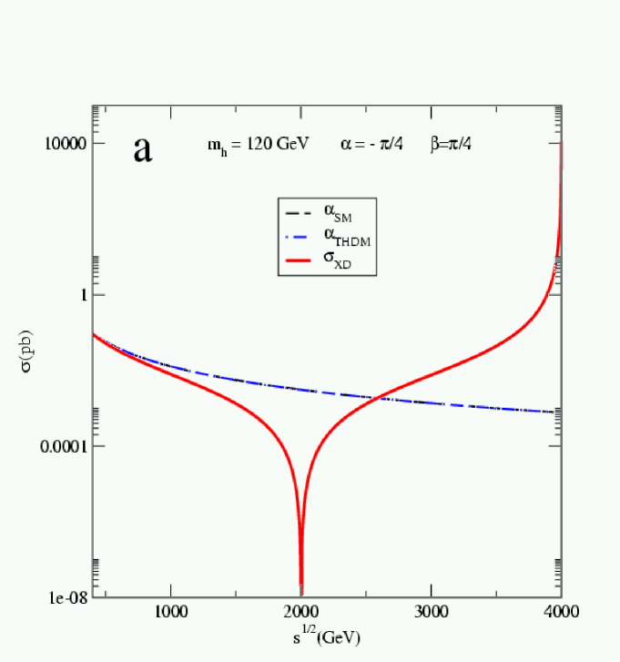
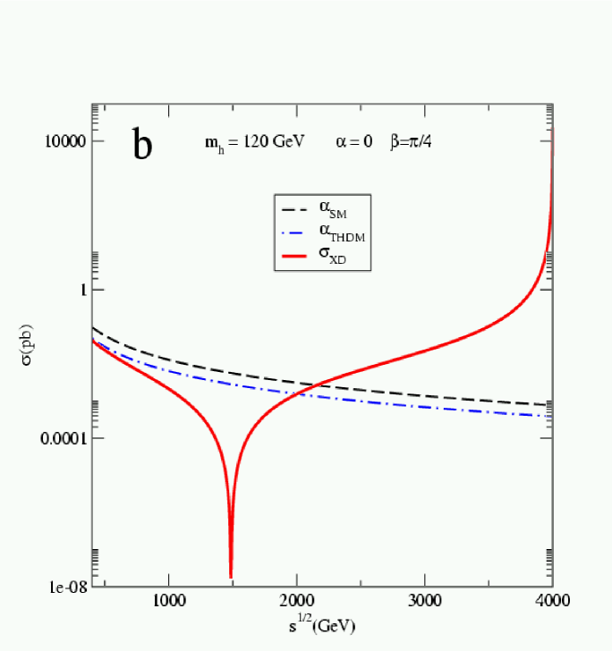
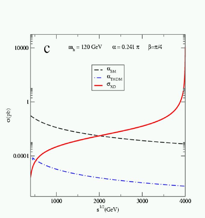
Figure 6.13: SM, THDM and XD cross Sections for $e^{+}e^{-}\rightarrow Zh$. Each plot corresponds to a different set of values for $\alpha$ and $\beta$, all with $m_{h}~{}=~{}120$ GeV and with a compactification scale $M_{c}~{}=~{}4$ TeV.

The Higgs discovery potential in this model is more promising at the LHC. We illustrate this in Fig. 6.14 showing the $pp\to hZ$ cross section as a function of the compactification scale $M_{c}$. One sees from the figure that depending on the particular values of $\alpha$ and $\beta$ the enhancement is more or less pronounced. But independently from the values of $\alpha$, $\beta$ (and the KK width), the XD production cross section is considerably enhanced with respect to the SM for $M_{c}\lesssim$ 6 TeV. For certain parameter values there is an enhancement even up to $M_{c}\sim$ 8 TeV.

The singularity at $RA(s)$ = 1 is regulated by the width of the KK mode, which is not included in our calculation. Thus, the peak region in Fig. 6.14 is only correct in the order of magnitude. Yet, since the width of the $n^{\rm th}$ KK mode $\Gamma_{n}\sim 2\alpha_{\rm em}m_{n}$ is rather small (since $\alpha_{\rm em}$ is small), the large enhancement is expected to prevail after the inclusion of the width. For particular $\alpha$ and $\beta$ values it might also happen that there is a cancellation among the terms containing the KK state information (see Ref. [21]). This cancellation also depends on the centre-of-mass energy ${\hat{s}}$ and $M_{c}$ and happens close to 8.5 TeV in Fig. 6.14.

In summary, we presented a model that accounts for the missing Higgs signal. Furthermore, the model promises an enhanced signal at the LHC or CLIC. It assumes one extra dimension and two Higgs doublets, one fixed to a brane and the other living in the bulk. The lightest CP-even scalar may be a mixing of the two and this non-trivial ‘location’ is the key ingredient in the suppression–enhancement of the discovery signal. We presented the results for the associated production cross sections at linear colliders and the LHC.

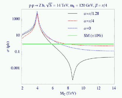
Figure 6.14: Higgs production cross section in association with a $Z$ boson as a function of the compactification scale for selected values of the mixing parameters. For reference the SM cross section is shown with a 10% uncertainty band around it.

6.1.5 Universal Extra Dimensions

Supersymmetry and extra dimensions offer two different paths to a theory of new physics beyond the SM. They both address the hierarchy problem, play a role in a more fundamental theory aimed at unifying the SM with gravity, and offer a candidate particle for dark matter, which is compatible with cosmological data. If either supersymmetry or extra dimensions exist at the TeV scale, signals of new physics are bound to be found by the ATLAS and CMS experiments at the LHC. However, the proper interpretation of such discoveries, namely the correct identification of the nature of the new physics signals, may not be straightforward at the LHC. It may have to be complemented by the data of a multi-TeV $e^{+}e^{-}$ colliders, such as CLIC [23].

A particularly interesting scenario is offered by Universal Extra Dimensions (UEDs), as originally proposed in [24]. It bears interesting analogies to supersymmetry, and has sometimes been referred to as ‘bosonic supersymmetry’ [25]. In principle, disentangling UED and supersymmetry may be highly non-trivial at hadron colliders. For each SM particle, they both predict the existence of a partner (or partners) with identical interactions. As the masses of these new particles are model-dependent, they cannot be used to discriminate between the two theories.

At the LHC, strong processes dominate the production in either case. The resulting signatures involve relatively soft jets, leptons and missing transverse energy [25]. The study in [25] shows that, with 100 fb^-1 of integrated luminosity, the LHC experiments will be able to cover all of the cosmologically preferred parameter space in UED [26]. However, the discrimination between UED and supersymmetry appears very difficult at the LHC.

In fact, there are only three fundamental differences between UED and supersymmetry. In the case of extra dimensions, there is an infinite tower of KK partners, labelled by their KK level $n$, while in supersymmetry, there is just a single superpartner for each SM particle. However, it is possible that the second and higher KK levels are too heavy to be observed. The second fundamental distinction between UED and supersymmetry is the fact that the KK partners have identical spin quantum numbers, while those of the superpartners differ by $1/2$. Unfortunately, spin determinations also appear to be difficult at the LHC. Finally, supersymmetry has an extended Higgs sector and gaugino states, which have no counterparts in the UED model. However, it is possible that these heavier Higgs bosons and gauginos are too heavy to be observed.

In its simplest incarnation, the UED model has all the SM particles propagating in a single extra dimension of size $R$, which is compactified on an $S_{1}/Z_{2}$ orbifold. A peculiar feature of UED is the conservation of the KK number at tree level, which is a simple consequence of momentum conservation along the extra dimension. However, bulk and brane radiative effects [27, 28, 29] break the KK number down to a discrete conserved quantity, the so-called KK parity, (–1)ⁿ, where $n$ is the KK level. KK parity ensures that the lightest KK partners — those at level one — are always pair-produced in collider experiments, similar to the case of supersymmetry models with conserved $R$-parity. KK-parity conservation also implies that the contributions to various precisely measured low-energy observables [30, 31, 32, 33, 34, 35, 36] only arise at the one-loop level and are small. In the minimal UED model, the boundary terms are assumed to vanish at the cutoff scale $\Lambda$, and are subsequently generated through RGE evolution to lower scales. Thus the minimal UED model has only two input parameters: the size of the extra dimension $R$ and the cutoff scale $\Lambda$.

In order to study the discrimination of UED signals from supersymmetry at CLIC, we concentrate on the pair production of level-1 KK muons $e^{+}e^{-}\to\mu^{+}_{1}\mu^{-}_{1}$, and compare it to the analogous process of smuon pair production in supersymmetry: $e^{+}e^{-}\to\tilde{\mu}^{+}\tilde{\mu}^{-}$. In UED there are two $n$ = 1 KK muon Dirac fermions: an $SU(2)_{W}$ doublet $\mu^{D}_{1}$ and an $SU(2)_{W}$ singlet $\mu^{S}_{1}$, both of which contribute. In complete analogy, in supersymmetry, there are two smuon eigenstates, $\tilde{\mu}_{L}$ and $\tilde{\mu}_{R}$, both of which contribute in $e^{+}e^{-}\to\tilde{\mu}^{+}\tilde{\mu}^{-}$.

We first fix the UED parameters to $R^{-1}$ = 500 GeV,   $R\Lambda$ = 20, corresponding to the spectrum given in Table 6.1.

Table 6.1: Masses of the KK excitations for the parameters $R^{-1}$ = 500 GeV and $\Lambda R$ = 20 used in the analysis

Particle		Mass
		(GeV)
$\mu_{1}^{D}$		515.0
$\mu_{1}^{S}$		505.4
$\gamma_{1}$		500.9

This analysis has backgrounds coming from SM $\mu^{+}\mu^{-}\nu\bar{\nu}$ final states, which are mostly due to gauge-boson pair production $W^{+}W^{-}\to\mu^{+}\mu^{-}\nu_{\mu}\bar{\nu}_{\mu}$, $Z^{0}Z^{0}\to\mu^{+}\mu^{-}\nu\bar{\nu}$ and from $e^{+}e^{-}\to W^{+}W^{-}\nu_{e}\bar{\nu}_{e}$, $e^{+}e^{-}\to Z^{0}Z^{0}\nu_{e}\bar{\nu}_{e}$, followed by muonic decays. The total cross Sections are $\simeq 20$ fb and $\simeq 2$ fb, respectively. In addition to its competitive cross section, this background has leptons produced preferentially at small polar angles, therefore biasing the UED/MSSM discrimination. In order to reduce the background, a suitable event selection has been applied based on the missing energy, the transverse energy and the event sphericity, which provides a factor $\simeq$ 5 background suppression in the kinematical region of interest. It does not bias the lepton-momentum distribution. The estimated background from $\gamma\gamma\to{\mathrm{hadrons}}$ appears to be negligible for muon energies above 2.5 GeV.

The angular distributions in UED and supersymmetry are sufficiently distinct to discriminate the two cases. However, the polar angles $\theta$ of the original KK muons and smuons are not directly observable, and the production polar angles $\theta_{\mu}$ of the final-state muons are measured instead. As long as the mass differences $M_{\mu_{1}}-M_{\gamma_{1}}$ and $M_{\tilde{\mu}}-M_{\tilde{\chi}^{0}_{1}}$, respectively, remain small, the muon directions are well correlated with those of their parents (see Fig. 6.15a).

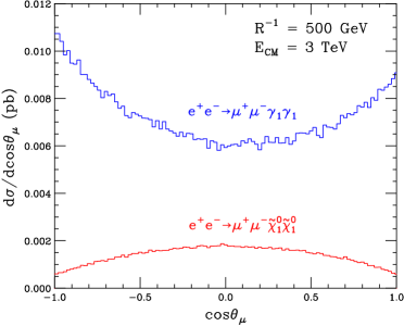
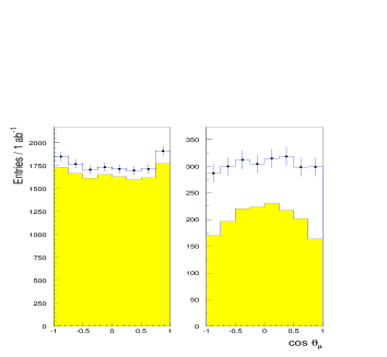
Figure 6.15: Differential cross section $d\sigma/d\cos\theta_{\mu}$ for UED (blue, top) and supersymmetry (red, bottom) as a function of the muon scattering angle $\theta_{\mu}$. We have chosen $R^{-1}$ = 500 GeV and $\Lambda R$ = 20 and then adjusted the SUSY-breaking parameters until we get a perfect spectrum match. The figure on the left is the ISR-corrected theoretical prediction, while the result on the right incorporates a detector simulation.

In Fig. 6.15b we show the same comparison after detector simulation and including the SM background. The angular distributions are still easily distinguishable after accounting for these effects. By performing a $\chi^{2}$ fit to the normalized polar-angle distribution, the UED scenario considered here could be distinguished from the MSSM, solely on the basis of the distribution shape, with 350 fb^-1 of data.

Further methods to distinguish between SUSY and UED are the production cross section and a threshold scan. The cross section for the UED processes rises at thresholds $\propto\beta$, while in supersymmetry their threshold onset is $\propto\beta^{3}$. Furthermore the cross section for the UED process is about 5 times larger compared to the smuon production in supersymmetry, for these masses.

The muon energy spectrum is completely determined by the kinematics of the two-body decay, and is therefore equivalent for the case of UED and of supersymmetry, if the relevant MSSM particle masses are properly tuned. We show the ISR-corrected expected distributions for the muon energy spectra at generator level in Fig. 6.16 (left), using the same parameters as in Fig. 6.15. We observe that the shape of the $E_{\mu}$ distribution in the case of the UED coincides with that for MSSM.

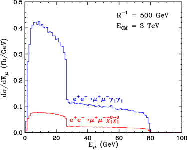
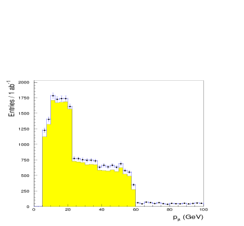
Figure 6.16: The muon energy spectrum resulting from KK muon production in UED (blue, top curve) and smuon production in supersymmetry (red, bottom curve), for the same UED and supersymmetry parameters in Fig. 6.15. The figure on the left is the ISR-corrected theoretical prediction, whilst the result on the right shows the distribution after detector simulation and including the background contribution.

In Fig. 6.16 (right) we show the muon energy distribution after detector simulation. The end-points can be used to extract the masses by a three-parameter fit to this distribution. A one-parameter fit, assuming the mass of the $\gamma_{1}$ state is known, gives an uncertainty on the $\mu_{1}$ mass of $\pm$ 0.25 GeV for 1 ab^-1 of statistics.

6.2 New Vector Resonances

Many scenarios of NP predict the existence of new particles that would manifest themselves as rather spectacular resonances in $e^{+}e^{-}$ collisions, if the achievable centre-of-mass energy is sufficient. A high-energy LC represents an ideal laboratory for studying this NP. Signals from NP that can be probed by a collider such as CLIC at 1 TeV $<\sqrt{s}<$ 5 TeV, belong to a rather large domain. The most striking manifestation of NP in the multi-TeV region would come from a sudden increase of the $e^{+}e^{-}\rightarrow f\bar{f}$ cross section indicating the $s$-channel production of a new particle. The experimental study of such resonances at a multi-TeV collider will have to accurately measure their masses, widths, production and decay properties to determine their nature and identify which kind of NP has been manifested. There are several theories that predict the existence of new vector resonances. A prominent class consists of models with extra gauge bosons such as a new neutral $Z^{\prime}$ gauge boson.

6.2.1 Extra-$Z^{\prime}$ Boson Studies

One of the simplest extensions of the SM consists of an additional $U(1)$ gauge symmetry broken at a scale close to the Fermi scale. This extra symmetry is predicted in both GUT-inspired $E_{6}$ models and in left–right-symmetric models. For example, in $E_{6}$ scenarios we have an additional $U(1)$ current $J_{Z^{\prime}\mu}^{f}=J_{\chi\mu}^{f}{\cos\theta_{6}}+J_{\psi\mu}^{f}{\sin\theta_{6}}$ with different models parametrized by specific values of the angle $\theta_{6}$. The values $\theta_{6}$ = 0, $\theta_{6}=\pi/2$ and $\theta_{6}=-\tan^{-1}\sqrt{5/3}$ are called the $\chi,\psi$ and $\eta$ models, respectively. In the LR models, the new $Z_{\rm LR}$ boson couples to the current $J_{Z^{\prime}\mu}=\alpha_{\rm LR}J_{3R\mu}-1/(2\alpha_{\rm LR})J_{(B-L)\mu}$ with $\alpha_{\rm LR}=\sqrt{g_{\rm R}^{2}/g_{\rm L}^{2}\cot^{2}\theta_{W}-1}$. The vector- and axial-vector couplings of the $Z^{\prime}$ boson to the SM fermions, for $E_{6}$-inspired and for LR models, are given in Table 6.2, assuming $J_{Z^{\prime}\mu}^{f}=\bar{f}\left[\gamma_{\mu}{v_{f}^{\prime}}+\gamma_{\mu}\gamma_{5}{a_{f}^{\prime}}\right]f$ and the parametrization $\theta_{2}=\theta_{6}+\tan^{-1}\sqrt{5/3}$. Finally, a useful reference is represented by the so-called sequential standard model (SSM), which introduces an extra $Z^{\prime}$ boson with the same couplings as the SM $Z^{0}$ boson.

Table 6.2: Vector and axial-vector couplings for the $E_{6}$-inspired and LR models, with $s_{\theta}=\sin\theta$, $s_{2}=\sin\theta_{2}$, $c_{2}=\cos\theta_{2}$, $c_{2\theta}=\cos 2\theta$, with $\theta_{2}=\theta_{6}+\tan^{-1}\sqrt{5/3}$ and $\theta\equiv\theta_{W}$

Extra-$U(1)$		LR $(g_{\rm L}=g_{\rm R})$
$v_{e}^{\prime}=-\frac{1}{4}s_{\theta}\left(c_{2}+\sqrt{\frac{5}{3}}s_{2}\right)$		$v_{e}^{\prime}=\left(-\frac{1}{4}+s_{\theta}^{2}\right)/\sqrt{c_{2\theta}}$
$a_{e}^{\prime}=\frac{1}{4}s_{\theta}\left(-\frac{1}{3}c_{2}+\sqrt{\frac{5}{3}}s_{2}\right)$		$a_{e}^{\prime}=-\frac{1}{4}\sqrt{c_{2\theta}}$
$v_{u}^{\prime}=0$		$v_{u}^{\prime}=\left(\frac{1}{4}-\frac{2}{3}s_{\theta}^{2}\right)/\sqrt{c_{2\theta}}$
$a_{u}^{\prime}=-\frac{1}{3}s_{\theta}c_{2}$		$a_{u}^{\prime}=\frac{1}{4}\sqrt{c_{2\theta}}$
$v_{d}^{\prime}=\frac{1}{4}s_{\theta}\left(c_{2}+\sqrt{\frac{5}{3}}s_{2}\right)$		$v_{d}^{\prime}=\left(-\frac{1}{4}+\frac{1}{3}s_{\theta}^{2}\right)/\sqrt{c_{2\theta}}$
$a_{d}^{\prime}=a_{e}^{\prime}$		$a_{d}^{\prime}=a_{e}^{\prime}$

There exist several constraints on the properties of new neutral vector gauge bosons. Direct searches for a new $Z^{\prime}$ boson set lower limits on the masses [37]. These are summarized in Table 6.3 for various models. An extra $Z^{\prime}$ naturally mixes with the SM $Z^{0}$ boson. The present precision electroweak data constrain the mixing angle $\theta_{M}$ within a few mrad, and the allowed masses are shown in Table 6.3 [39, 38].

Table 6.3: The 95% C.L. limits on $M_{Z^{\prime}}$ (GeV) from $\sigma(pp\to Z^{\prime})B(Z^{\prime}\to ll)$ (CDF data) and from the average of the four LEP experiments, for the mixing angle $\theta_{M}$ = 0

		$\chi$	$\psi$	$\eta$	$LR$	SSM
CDF		595	590	620	630	690
LEP		673	481	434	804	1787

A third class of constraints can be derived from the atomic-parity violation (APV) data [40, 20], since models involving extra neutral vector bosons can modify the $Q_{W}$ value significantly. The present value of $Q_{W}$ extracted from the caesium data differs by only $\simeq$ 0.8$\sigma$ from the SM prediction. We note that there exist improved predictions of $Q_{W}$ in the SM, which account for the effect of the Breit interaction among electrons and have a refined calculation of the radiative corrections [41].

Assuming no $Z^{0}$–$Z^{\prime}$ mixing, we can evaluate the contribution to the weak charge due to the direct exchange of the $Z^{\prime}$ and derive bounds on $M_{Z^{\prime}}$. The 95% C.L. limit from APV on $M_{Z^{\prime}}$ for the $\chi$, $\eta$, LR and SSM models are 627, 476, 665 and 1010 GeV respectively [20], while no bounds can be set on the $\psi$ model by the APV measurements. These are less stringent than, or comparable to, those from the LEP experiments. However, as these bounds are very sensitive to the actual value of $Q_{W}$ and its uncertainties, further determinations may improve the sensitivity.

The LHC will push the direct sensitivity to new vector gauge bosons past the TeV threshold. With an integrated luminosity of 100 fb^-1, ATLAS and CMS are expected to observe signals from $Z^{\prime}$ bosons for masses up to 4–5 TeV, depending on the specific model [42].

Extra-$U(1)$ models can be accurately tested at CLIC. With an expected effective production cross section $\sigma(e^{+}e^{-}\to Z^{\prime}_{SSM})$ of $\simeq$ 15 pb, including the effects of ISR and luminosity spectrum, a $Z^{\prime}$ resonance will tower over a $q\bar{q}$ continuum background of $\simeq$ 0.13 pb. Whilst the observability of such a signal is guaranteed, the accuracy that can be reached in the study of its properties depends on the quality of the accelerator beam-energy spectrum and on the detector response, including accelerator-induced backgrounds. One of the main characteristics of the CLIC collider is the large design luminosity, $L$ = 10³⁵ cm^-2 s^-1 at $\sqrt{s}$ = 3 TeV for its baseline parameters, obtained in a regime of strong beamstrahlung effects. The optimization of the total luminosity and its fraction in the peak has been studied for the case of a resonance scan. The CLIC luminosity spectrum has been obtained with a dedicated beam simulation program [43], as discussed in Chapter 3, for the nominal parameters at $\sqrt{s}$ = 3 TeV. In order to study the systematic uncertainties in the knowledge of this spectrum, the modified Yokoya–Chen parametrization [44] has been adopted. In this formulation, the beam energy spectrum is described in terms of $N_{\gamma}$, the number of photons radiated per $e^{\pm}$ in the bunch, the beam energy spread in the linac $\sigma_{p}$ and the fraction $\cal{F}$ of events outside the 0.5% of the centre-of-mass energy. Two sets of parameters have been considered, obtained by modifying the beam size at the interaction point and therefore the total luminosity and its fraction in the highest energy region of the spectrum: CLIC.01 with ${\cal{L}}$ = 1.05 $\times$ 10³⁵ cm^-2 s^-1 and $N_{\gamma}$ = 2.2 and CLIC.02 with ${\cal{L}}$ = 0.40 $\times$ 10³⁵ cm^-2 s^-1 and $N_{\gamma}$ = 1.2. The $Z^{\prime}$ mass and width can be determined by performing either an energy scan, like the $Z^{0}$ line-shape scan performed at LEP/SLC, or an autoscan, by tuning the collision energy just above the top of the resonance and profiting from the long tail of the luminosity spectrum to probe the resonance peak.

For the first method, both dijet and dilepton final states can be considered, while for the autoscan only $\mu^{+}\mu^{-}$ final states can provide the necessary accuracy for the $Z^{\prime}$ energy. We have generated $e^{+}e^{-}\rightarrow Z^{\prime}$ events for $M_{Z^{\prime}}$ = 3 TeV, including the effects of ISR, the luminosity spectrum and $\gamma\gamma$ backgrounds, assuming SM-like couplings, corresponding to a total width $\Gamma_{Z^{\prime}_{SSM}}\simeq$ 90 GeV. The resonance widths for extra-$U(1)$ models as well as for other SM extensions with additional vector bosons are shown in Fig. 6.17 as a function of the relevant model parameters.

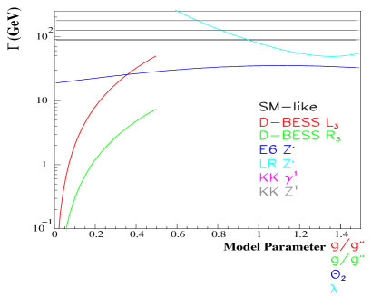
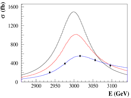
Figure 6.17: Left: Widths of new gauge vector bosons as functions of the relevant parameters: $\theta_{2}$ for $Z^{\prime}_{E_{6}}$, $\lambda=g_{\rm L}/g_{\rm R}$ for $Z^{\prime}_{\rm LR}$ [45], $g/g^{\prime\prime}$ for D-BESS. The KK $Z^{(1)}$ width has a negligible dependence on the mixing angle $\sin\beta$. The $Z^{\prime}_{E_{6}}$ and $Z^{\prime}_{\rm LR}$ widths are computed by assuming only decays into SM fermions. Right: The $Z^{\prime}_{\rm SSM}\to\ell^{+}\ell^{-}$ resonance profile obtained by an energy scan. The Born production cross section, the cross section with ISR included and that accounting for the CLIC luminosity spectrum (CLIC.01) and tagging criteria are shown.

A data set of 1 ab^-1 has been assumed for the CLIC.01 beam parameters and of 0.4 ab^-1 for CLIC.02, corresponding to one year ( = 10⁷ s) of operation at nominal luminosity. This has been shared in a five-point scan, as seen in Fig. 6.17, and $M_{Z^{\prime}}$, $\Gamma_{Z^{\prime}}/\Gamma_{Z^{0}}$ and $\sigma_{\rm peak}$ have been extracted from a $\chi^{2}$ fit to the predicted cross section behaviour for different mass and width values (see Table 6.4) [46]. The dilution of the analysing power due to the beam energy spread is appreciable, as can be seen by comparing the statistical accuracy from a fit to the pure Born cross section after including ISR and beamstrahlung effects. Still, the relative statistical accuracies are better than 10^-4 on the mass and 5 $\times$ 10^-3 on the width. In the case of wide resonances, there is an advantage in employing the broader luminosity spectrum of CLIC.01, which offers larger luminosity. Sources of systematics from the knowledge of the shape of the luminosity spectrum have also been estimated. In order to keep $\sigma_{\rm syst}\leq\sigma_{\rm stat}$ it is necessary to control $N_{\gamma}$ to better than 5% and the fraction $\cal{F}$ of collisions at $\sqrt{s}<$ 0.995 $\sqrt{s_{0}}$ to about 1% [47].

Table 6.4: Results of fits for the cross-Section scan of a $Z^{\prime}_{\rm SSM}$ obtained by assuming no radiation and ISR with the effects of two different choices of the CLIC luminosity spectrum

Observable	Breit–Wigner	CLIC.01	CLIC.02
$M_{Z^{\prime}}$ (GeV)	3000 $\pm$ .12	$\pm$ .15	$\pm$ .21
$\Gamma_{Z^{\prime}}/\Gamma_{Z^{0}}$	1. $\pm$ .001	$\pm$ .003	$\pm$ .004
$\sigma^{\rm eff}_{\rm peak}$ (fb)	1493 $\pm$ 2.0	564 $\pm$ 1.7	669 $\pm$ 2.9

6.2.2 Heavy Majorana Neutrinos in $Z^{\prime}$ Decays

If neutrinos are Majorana particles, then the left–right-symmetric model and the see-saw mechanism [48] may provide an explanation for the lightness of the left-handed neutrinos, by introducing heavy right-handed neutrinos, $N_{l}$. The LHC is expected to discover these new particles after three years of operation at high luminosity, mostly through $pp\rightarrow W_{R}\rightarrow lN_{l}$, if $m(N_{l})$ and $m(W_{R})$ are smaller than 4 and 6 TeV, respectively [49]. At CLIC, the resonant production of $Z^{\prime}_{\rm LR}\rightarrow N_{e}N_{e}$ may lead to signal rates up to about three orders of magnitude higher than for $pp\rightarrow Z^{\prime}_{\rm LR}\rightarrow N_{e}N_{e}$ at LHC energies. This process has been studied using the fast detector simulation [50]. Since $N_{e}$ is expected to decay promptly into $e^{\pm}$ and a $q_{i}\bar{q}_{j}$ pair, two electrons of equal charge and four quarks in the final state are the decay signature. The $\gamma\gamma$ background may induce a shift of the $Z^{\prime}$ and $N_{e}$ invariant mass peaks towards higher masses. In order to reduce this effect a kinematical fit can be applied after the reconstruction procedure. It requires that the two $N_{e}$ candidates have equal mass, the system consisting of the two electrons and the four leading hadronic jets have a zero transverse momentum, the momentum and energy conservation at $\sqrt{s}$ = 3 TeV. These corrections allow a good reconstruction of $Z^{\prime}_{\rm LR}$ and $N_{e}$, as shown in Fig. 6.18.

Figure 6.18: Signature of Majorana neutrinos. The left plot shows the reconstructed 3 TeV $Z^{\prime}$ boson before and after the kinematical fit, and the right plot shows the reconstructed 1 TeV Majorana neutrino before and after the kinematical fit for an integrated luminosity of 1 ab^-1.

6.3 Indirect Sensitivity to New Physics

The direct reach for the mass scales of new phenomena provided by CLIC are in many cases comparable to those provided by the LHC. However, CLIC would be able to explore more details of any new processes, possibly allowing one to determine better the nature of the new physics discovered. With the centre-of-mass energies and the luminosity envisioned for CLIC, a new era of precision physics is approaching. Precision electroweak measurements performed in multi-TeV $e^{+}e^{-}$ collisions will push the indirect sensitivity to new mass scales beyond the 10 TeV frontier.

We review here the sensitivity to new gauge bosons $Z^{\prime}$, to KK excitations of the SM gauge bosons and to contact interactions [51, 46], as examples of the anticipated potential of CLIC. These results are based on studies of the two-fermion ($\mu^{+}\mu^{-}$, $b\bar{b}$ and $t\bar{t}$) production cross sections, $\sigma_{f\bar{f}}$, and forward–backward asymmetries, $A_{\rm FB}^{f\bar{f}}$.

At CLIC design centre-of-mass energies, the relevant $e^{+}e^{-}\rightarrow f\bar{f}$ cross sections are significantly reduced with respect to those at present-day energies, and the experimental conditions in the interaction region need to be taken into account in validating the accuracies on electroweak observables. Since two-fermion cross sections are of the order of only 10 fb, it is imperative to operate the collider at high luminosity. This can be achieved only in a regime where beam–beam effects are important and primary $e^{+}e^{-}$ collisions are accompanied by several $\gamma\gamma\rightarrow hadrons$ interactions. Being mostly confined in the forward regions, this $\gamma\gamma$ background reduces the polar-angle acceptance for quark-flavour tagging, and dilutes the possible jet-charge separation. These experimental conditions require efficient and robust algorithms to ensure sensitivity to flavour-specific $f\bar{f}$ production.

The statistical accuracies for the determination of $\sigma_{f\bar{f}}$ and $A_{\rm FB}^{f\bar{f}}$ have been studied using a realistic simulation. For example, the identification of $b\bar{b}$ final states was based on the sampling of the charged multiplicity in decays of highly-boosted $b$ hadrons at CLIC energies [52]. Similarly to LEP analyses, the forward–backward asymmetry for $b\bar{b}$ has been extracted from a fit to the flow of the jet charge $Q^{\rm jet}$, defined as $Q^{\rm jet}=\frac{\sum_{i}q_{i}|\vec{p}_{i}\cdot\vec{T}|^{k}}{\sum_{i}|\vec{p}_{i}\cdot\vec{T}|^{k}}$, where $q_{i}$ is the particle charge, $\vec{p}_{i}$ its momentum, $\vec{T}$ the jet thrust unit vector, $k$ a positive number, and the sum is extended to all the particles in a given jet. Here the presence of additional particles, from the $\gamma\gamma$ background, causes a broadening of the $Q^{\rm jet}$ distribution and thus a dilution of the quark charge separation. The track selection and the value of the power parameter $k$ need to be optimized as a function of the number of overlaid bunch crossings. Results for the $e^{+}e^{-}\to\bar{t}t$ channel have been obtained using a dedicated top tagging algorithm [53]. This uses an explicit reconstruction of the $t\to bW$ decay and also includes the physics and machine-induced backgrounds. For $t\bar{t}$ forward–backward asymmetries, the sign of the lepton from the $W^{\pm}\to\ell^{\pm}\nu$ decay has been used. The results are summarized in terms of the relative statistical accuracies $\delta{\cal{O}}/{\cal{O}}$ in Table 6.5.

Table 6.5: Relative statistical accuracies on electroweak observables obtainable for 1 ab^-1 of CLIC data at $\sqrt{s}$ = 3 TeV, including the effect of the $\gamma\gamma\to hadrons$ background

Observable		Relative stat. accuracy
		$\delta{\cal{O}}/{\cal{O}}$ for 1 ab-1
$\sigma_{\mu^{+}\mu^{-}}$		$\pm$ 0.010
$\sigma_{b\bar{b}}$		$\pm$ 0.012
$\sigma_{t\bar{t}}$		$\pm$ 0.014
$A_{\rm FB}^{\mu\mu}$		$\pm$ 0.018
$A_{\rm FB}^{bb}$		$\pm$ 0.055
$A_{\rm FB}^{tt}$		$\pm$ 0.040

However, it is important to stress that, at the energy scales considered here, electroweak virtual corrections are strongly enhanced by Sudakov double logarithms of the type $\log^{2}(s/M_{W}^{2})$. Until a complete two-loop result settles the problem, a theoretical error on the cross Section of the order of a per cent could be considered [54]. We have not included it in the present analyses. This issue is discussed in detail in the next section.

The indirect sensitivity of a LC to the $Z^{\prime}$ mass $M_{Z^{\prime}}$ can be parametrized in terms of the available integrated luminosity ${\cal{L}}$ and the centre-of-mass energy $\sqrt{s}$. A scaling law for large $M_{Z^{\prime}}$ can be obtained by considering the effect of the $Z^{\prime}$–$\gamma$ interference in the cross section. For $s\ll M_{Z^{\prime}}^{2}$ and assuming that the uncertainties $\delta\sigma$ are statistically dominated, we can infer the range of mass values that would give a significant difference from the SM prediction:

$$\frac{|\sigma^{\rm SM}-\sigma^{\rm{SM}+Z^{\prime}}|}{\delta\sigma}\propto\frac{1}{M^{2}_{Z^{\prime}}}\sqrt{s{\cal{L}}}>\sqrt{\Delta\chi^{2}},$$ (6.2)

and the sensitivity to the $Z^{\prime}$ mass scales as:

$$M_{Z^{\prime}}\propto(s{\cal{L}})^{1/4}.$$ (6.3)

This relation points to the direct trade-off possible between $\sqrt{s}$ and ${\cal{L}}$. This needs to be taken into account in the optimization of the parameters of a high-energy $e^{+}e^{-}$ linear collider.

The $\sigma_{f\bar{f}}$ and $A_{\rm FB}^{f\bar{f}}$ ($f=\mu,~{}b,~{}t$) values have been computed for 1 TeV $<\sqrt{s}<$ 5 TeV, both in the SM and including the corrections due to the presence of a $Z^{\prime}$ boson with 10 TeV $<M_{Z^{\prime}}<$ 40 TeV, with couplings defined by the models discussed in Section 2. Predictions have been obtained by implementing these models in the Comphep program [55]. Relative statistical errors on the electroweak observables are obtained by rescaling the values of Table 6.5 for different energies and luminosities. The sensitivity has been defined as the largest $Z^{\prime}$ mass, giving a deviation of the actual values of the observables from their SM predictions corresponding to a SM probability of less than 5%. The SM probability has been defined as the minimum of the global probability computed for all the observables and that for each of them taken independently.

This sensitivity has been determined, as a function of the $\sqrt{s}$ energy and integrated luminosity ${\cal{L}}$, and compared to the scaling in (6.3). Results are summarized in Fig. 6.19. For the $\eta$ model the sensitivity is lower. To reach the sensitivity of $M_{Z^{\prime}}$ = 20 TeV, more than 10 ab^-1 of data at $\sqrt{s}$ = 5 TeV are necessary.

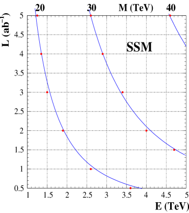
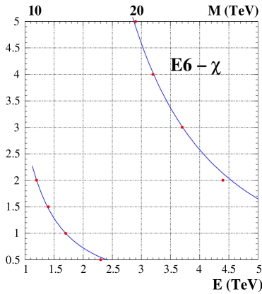
Figure 6.19: The 95% C.L. sensitivity contours in the ${\cal{L}}$ vs. $\sqrt{s}$ plane for different values of $M_{Z^{\prime}}$ in the SSM model (left) and in the $E_{6}$ $\chi$ model (right). The points represent the results of the analysis, while the curves show the behaviour expected from the scaling suggested in (6.3).

In the case of the 5D SM, we have included only the effects of the exchange of the first KK excitations $Z^{(1)}$ and $\gamma^{(1)}$, neglecting those of the remaining excitations of the towers, which give only small corrections. The scaling law for the limit on $M$ can be obtained by considering the interference of the two new nearly degenerate gauge bosons with the photon in the cross section and taking the $s\ll M^{2}$ limit. The result is the same as (6.3). The analysis closely follows that for the $Z^{\prime}$ boson discussed above. In Fig. 6.20 we give the sensitivity contours as a function of $\sqrt{s}$ for different values of $M$. We conclude that the achievable sensitivity to the compactification scale $M$ for an integrated luminosity of 1 ab^-1 in $e^{+}e^{-}$ collisions at $\sqrt{s}$ = 3–5 TeV is of the order of 40–60 TeV. Results of a similar analysis, including all electroweak observables, are discussed in Ref. [56].

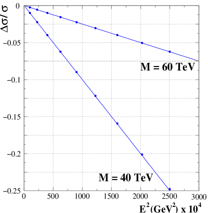
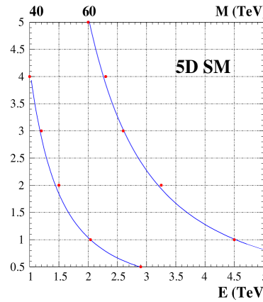
Figure 6.20: Left: Scaling of the relative change in the $e^{+}e^{-}\to b\bar{b}$ cross section, in the 5D SM, as a function of the square of the centre-of-mass energy, for two values of the compactification scale $M$. Right: The 95% C.L. sensitivity contours in the ${\cal{L}}$ vs. $\sqrt{s}$ plane for different values of the compactification scale $M$ in the 5D SM. The points represent the results of the analysis, while curves show the behaviour expected from the scaling suggested in (6.3).

An important issue concerns the ability to probe the models, if a significant discrepancy from the SM predictions were to be observed. Since the model parameters and the mass scale are a priori arbitrary, an unambiguous identification of the realized scenario is difficult. However, some information can be extracted by testing the compatibility of different models while varying the mass scale. Figure 6.21 shows an example of such a test. Taking $M$ = 20 TeV, ${\cal{L}}$ = 1 ab^-1 of CLIC data at $\sqrt{s}$ = 3 TeV could distinguish the SSM model from the $E_{6}$ $\chi$ model at 86% C.L. and from the 5D SM at 99% C.L. For a mass scale of 40 TeV, ${\cal{L}}$ = 3 ab^-1 of CLIC data at $\sqrt{s}$ = 5 TeV, the corresponding confidence levels become 91% and 99%, respectively. Further sensitivity to the nature of the gauge bosons could be obtained by studying the polarized forward–backward asymmetry $A_{\rm FB}^{\rm pol}$ and the left–right asymmetry $A_{\rm LR}$ using colliding polarized beams.

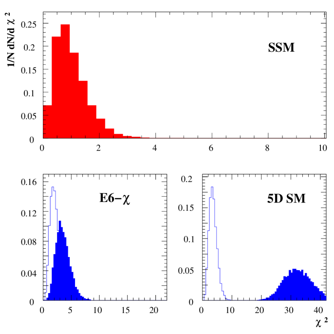
Figure 6.21: The $\chi^{2}$ distributions obtained for a set of pseudo-experiments where the SSM is realized with a mass $M_{Z^{\prime}}$ of 20 TeV (upper plot). The corresponding distributions for the $E(6)$ $\chi$ and 5D SM for the same mass scale (full histograms) and for $M$ = 40 TeV are also shown for comparison in the lower panels. By integrating these distributions, one obtains the confidence levels for discriminating between these models that are discussed in the text.

The scenarios investigated above address specific models of new physics beyond the SM. Fermion compositeness or exchanges of very heavy new particles can be described in all generality by four-fermion contact interactions [57]. These parametrize the interactions beyond the SM in terms of an effective scale $\Lambda_{ij}$:

$${\cal L}_{\rm CI}=\sum_{i,j=\mathrm{L,R}}\eta_{ij}\frac{g^{2}}{\Lambda^{2}_{ij}}(\bar{e_{i}}\gamma^{\mu}e_{i})(\bar{f_{j}}\gamma^{\mu}f_{j})\,.$$ (6.4)

The strength of the interaction is set by convention as $g^{2}/4\pi$ = 1, and models can be considered by choosing either $|\eta_{ij}|$ = 1 or $|\eta_{ij}|$ = 0 as detailed in Table 6.6. The contact scale $\Lambda$ can be interpreted as an effect of new particles at a mass $M_{X}$: $1/\Lambda^{2}\propto\lambda^{2}/M_{X}^{2}$.

Table 6.6: Definition of different models of contact interaction

Model	LL	RR	LR	RL	VV	AA	V0	A0
$\eta_{\mathrm{LL}}$	$\pm$ 1	0	0	0	$\pm$ 1	$\pm$ 1	$\pm$ 1	0
$\eta_{\mathrm{RR}}$	0	$\pm$ 1	0	0	$\pm$ 1	$\pm$ 1	$\pm$ 1	0
$\eta_{\mathrm{LR}}$	0	0	$\pm$ 1	0	$\pm$ 1	$\mp$ 1	0	$\pm$ 1
$\eta_{\mathrm{RL}}$	0	0	0	$\pm$ 1	$\pm$ 1	$\mp$ 1	0	$\pm$ 1

In order to estimate the sensitivity of electroweak observables to the contact interaction scale $\Lambda$, the statistical accuracies discussed in Table 6.5 have been assumed for the $\mu\mu$ and $b\bar{b}$ final states. The assumed systematics of 0.5% include the contributions from model prediction uncertainties. Results are given in terms of the lower limits on $\Lambda$, which can be excluded at 95% C.L., in Fig. 6.22. It has been verified that, for the channels considered in the present analysis, the bounds for the different $\Lambda_{ij}$ are consistent. High-luminosity $e^{+}e^{-}$ collisions at 3 TeV can probe $\Lambda$ at scales of 200 TeV and beyond. For comparison, the corresponding results expected for a LC operating at 1 TeV are also shown. Beam polarization represents an important tool in these studies. First, it improves the sensitivity to new interactions, through the introduction of the left–right asymmetries $A_{\rm LR}$ and the polarized forward–backward asymmetries $A_{\rm FB}^{\rm pol}$ in the electroweak fits. If both beams can be polarized to ${\cal{P}}_{-}$ and ${\cal{P}}_{+}$ respectively, the relevant parameter is the effective polarization defined as ${\cal{P}}=\displaystyle{\frac{-{\cal{P}}_{-}+{\cal{P}}_{+}}{1-{\cal{P}}_{-}+{\cal{P}}_{+}}}$. In addition to the improved sensitivity, the uncertainty on the effective polarization can be made smaller than the error on the individual beam polarization measurements. Secondly, if a significant deviation from the SM prediction were to be observed, $e^{-}$ and $e^{+}$ polarization is greatly beneficial to a determination of the nature of the new interactions. This has been studied in detail for a LC at 0.5–1.0 TeV [58], and those results also apply, qualitatively, to a multi-TeV collider.

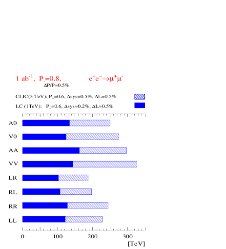
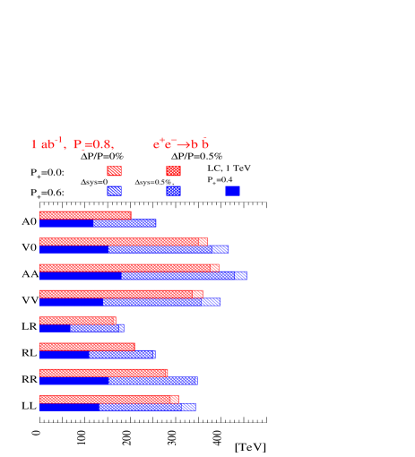
Figure 6.22: Limits on the scale $\Lambda$ of contact interactions for CLIC operating at 3 TeV (dashed histogram) compared with a 1 TeV LC (filled histogram) for different models and the $\mu^{+}\mu^{-}$ (left) and $b\bar{b}$ (right) channels. The polarization of electrons ${\cal{P}}_{-}$ is taken to be 0.8 and that of positrons ${\cal{P}}_{+}$ = 0.6. For comparison, the upper bars in the right plot show the sensitivity achieved without positron polarization. The influence of systematic uncertainties is also shown.

Using the scaling law, the expected gain in reach on $\Lambda$ for 5 ab^-1 and a 5 TeV (10 TeV) $e^{+}e^{-}$ collider would be 400–800 GeV (500–1000 GeV). This is a very exciting prospect, if for the ‘doomsday’ scenario where in some years from now only a light Higgs has been discovered, and no sign of other new physics has been revealed by the LHC or a TeV-class LC. Indeed, if the Higgs particle is light, i.e. below 150 GeV or so, then the SM cannot be stable up to the GUT or Planck scale, and a new mechanism is needed to stabilize it, as shown in Fig. 6.23 [59]: only a narrow corridor of Higgs masses around 180 GeV allow an extrapolation of the SM up to the Planck scale without introduction of any new physics. For example, for a Higgs with a mass in the region of 115–120 GeV, the SM will hit a region of electroweak unstable vacuum in the range of 100–1000 TeV. Hence, if the theoretical assessment of Fig. 6.23 remains valid, and the bounds do not change significantly (which could happen following a change in the top-quark mass from, e.g. new measurements at the Tevatron) and the Higgs is as light as 120 GeV, then the signature of new physics cannot escape precision measurements at CLIC.

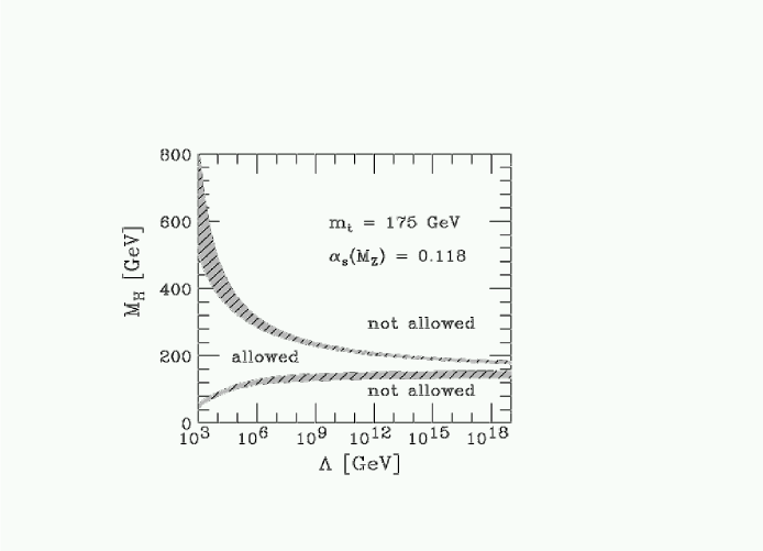
Figure 6.23: The range allowed for the mass of the Higgs boson if the SM is to remain valid up to a given scale $\Lambda$. In the upper part of the plane, the effective potential blows up, whereas in the lower part the present electroweak vacuum is unstable [59].

Finally, we note that straightforward left–right asymmetry measurements in Møller scattering, as observed in $e^{-}e^{-}$ interactions, can be used as sensitive probes of new physics effects due to, say, the existence of higher-mass $Z^{\prime}$ bosons, doubly-charged scalars (which might belong to an extended Higgs sector), or the presence of extra dimensions [60]. The running of $\sin^{2}\theta_{W}$ with $Q^{2}$ can be measured over a large parameter range to probe for such novel effects, in a single experiment. The added energy reach of CLIC will be of major importance for the sensitivity of such studies. As an example: assuming 90% polarized beams at a CLIC energy of 3 TeV, $e^{-}e^{-}$ interactions will be sensitive to interference effects up to a compositeness scale of $\sim 460$ TeV, far outdistancing the Bhabha scattering sensitivity even if the electron (but not the positron) is polarized. For the same integrated luminosity, the sensitivity to $\Lambda$ is about a factor 1.6 larger in $e^{-}e^{-}$ scattering, compared with $e^{+}e^{-}$ scattering.

6.3.1 Triple-Gauge-Boson Couplings

Another example of precision measurements is the determination of triple-gauge-boson couplings (TGCs), studied, e.g. via $e^{+}e^{-}\rightarrow W^{+}W^{-}$. An important feature of the electroweak SM is the non-Abelian nature of its gauge group, which gives rise to gauge-boson self-interactions, in particular to TGCs. A precision measurement of these interactions at high energies will be a crucial test of the validity of the SM, given that many of its extensions predict deviations, typically through the effects of new particles and couplings in radiative corrections: see Ref. [61], for example.

An initial study using TeV-class LC results for background and detector effects suggests that the sensitivity to the anomalous $\Delta\lambda_{\gamma}$ and $\Delta\kappa_{\gamma}$ couplings (which are zero in the SM) for CLIC at 3 (5) TeV amounts to roughly 1.3 $\times$ 10^-4 (0.8 $\times$ 10^-4) and 0.9 $\times$ 10^-4 (0.5 $\times$ 10^-4) respectively, for 1 ab^-1 of data [62]. A comparative study is shown in Fig. 6.24. The TGC errors are statistical only, but only $e$ and $\mu$ semileptonic $WW$ events have been included in the analysis. It has been argued heuristically that the statistical error from $e$ and $\mu$ semileptonic $WW$ events approximates well the total statistical and systematic error that is obtained when all $WW$ events are analysed. This was shown to be true at LEP 2, and was also found to be true in a complete analysis of TGCs for a $\sqrt{s}$ = 500 GeV analysis. We infer that a multi-TeV collider such as CLIC could probe these couplings a factor 2–4 times more precisely than a TeV-class LC.

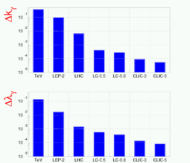
Figure 6.24: Precision of triple gauge coupling (TGC) measurements at different accelerators, for one year of high-luminosity data taking [62]

Allowing for complex couplings, in a form factor approach the most general $\gamma WW$ and $ZWW$ vertex functions lead to 28 real parameters altogether [63]. All four LEP collaborations have investigated TGCs and found agreement with the SM. The 68% C.L. errors for the combined results [64] are of order 0.02 for $g_{1}^{Z}$ and $\lambda_{\gamma}$, and of order 0.06 for $\kappa_{\gamma}$. The tightest constraints for the real and imaginary parts of $C$- and/or $P$-violating couplings [65, 66, 67] are of order 0.1 to 0.6. All these values correspond to single-parameter fits. Since only fits with up to three parameters have been performed, only a small subset of couplings has been considered at a time, thereby neglecting possible correlations between most of them. Moreover, many couplings, notably the imaginary parts of $C$- and $P$-conserving couplings, have so far been dropped from the experimental analyses.

At a future linear $e^{+}e^{-}$ collider one will be able to study these couplings with unprecedented accuracy. A process particularly suitable for this is $W$ pair production, where both the $\gamma WW$ and $ZWW$ couplings can be measured at the scale given by the centre-of-mass energy $\sqrt{s}$.

Given the intricacies of a multidimensional parameter space, the full covariance matrix for the errors on all 28 couplings should be studied. The high statistics needed for that is available both at a first-generation LC in the 1-TeV range and at a multi-TeV machine like CLIC. With an integrated luminosity of 3 ab^-1 and unpolarized beams at $\sqrt{s}$ = 3 TeV, about 1.5 million $W$ pairs are produced before cuts.

In experimental analyses of TGCs and various other processes, optimal observables [68] have proved to be a useful tool to extract physics parameters from the event distributions. These observables are constructed so as to have the smallest possible statistical errors. Thanks to this property, they are also a convenient means of determining the theoretically achievable sensitivity in a given process. In addition, they take advantage of the discrete symmetries of the cross Section. In $W$ pair production, the covariance matrix of these observables consists of four blocks that correspond to CP-even or CP-odd TGCs and to their real and imaginary parts. For this process it is convenient to use the following parameters:

$$g_{1}{\rm{}^{L}} = 4\sin^{2}\theta_{W}\,g_{1}^{\gamma}+(2-4\sin^{2}\!\theta_{W})\,\xi\,g_{1}^{Z}\,,$$ (6.5)

$$g_{1}^{\rm R} = 4\sin^{2}\theta_{W}\,g_{1}^{\gamma}-4\sin^{2}\!\theta_{W}\,\xi\,g_{1}^{Z}\,,$$

and similarly for the other couplings, where $\xi=s/(s-m_{Z}^{2})$. The linear combinations are chosen such that the couplings $h^{\rm L}$ ($h^{\rm R}$) occur in the amplitudes of left- (right-) handed $e^{-}$ and right- (left-) handed $e^{+}$. With unpolarized beams one mainly measures the $h^{\rm L}$, which are strongly enhanced by the interference with neutrino exchange in the $t$ channel. Table 6.7 shows the achievable errors on the real parts of the couplings in the presence of all TGCs [61]. Notice the increase in sensitivity for higher energies, especially for ${\rm Re}\,\Delta\kappa_{\rm L,R}$, ${\rm Re}\,\lambda_{\rm L,R}$ and ${\rm Re}\,\tilde{\lambda}_{\rm L,R}$.

Table 6.7: Errors on the real parts of CP-even (top) and -odd (bottom) couplings for different centre-of-mass energies in units of 10^-3. The assumed integrated luminosities are 500 fb^-1, 1 ab^-1 and 3 b^-1 at $\sqrt{s}$ = 500 GeV, 800 GeV and 3 TeV, respectively. Only those final states are considered where one $W$ decays into a quark–antiquark pair and the other into $e\nu$ or $\mu\nu$. These are the errors that can be obtained in the presence of all 28 TGCs (the covariance matrices are not shown).

$\sqrt{s}$ (GeV)	Re $\Delta g_{1}^{\rm L}$	Re $\Delta\kappa_{\rm L}$	Re $\lambda_{\rm L}$	Re $g_{5}^{\rm L}$	Re $\Delta g_{1}^{\rm R}$	Re $\Delta\kappa_{\rm R}$	Re $\lambda_{\rm R}$	Re $g_{5}^{\rm R}$
500	2.6	0.85	0.59	2.0	10	2.4	3.6	6.7
800	1.6	0.35	0.24	1.4	6.2	0.92	1.8	4.8
3000	0.93	0.051	0.036	0.88	3.1	0.12	0.36	3.2

$\sqrt{s}$ (GeV)	Re $\Delta g_{4}^{\rm L}$	Re $\tilde{\lambda}_{\rm L}$	Re $\tilde{\kappa}_{\rm L}$	Re $\Delta g_{4}^{\rm R}$	Re $\tilde{\lambda}_{\rm R}$	Re $\tilde{\kappa}_{\rm R}$
500	2.5	0.60	2.7	10	3.8	11
800	1.7	0.24	1.8	6.5	1.8	6.8
3000	0.90	0.036	0.97	3.4	0.36	3.2

The sensitivity to anomalous TGCs changes considerably in the presence of initial beam polarization. With longitudinally-polarized beams, the strength of the neutrino exchange can in essence be varied freely. In Table 6.8 we give the errors $\delta h$ on the real

Table 6.8: Errors in the real parts of CP-even couplings at $\sqrt{s}$ = 3 TeV for different initial beam polarizations in units of 10^-3

$P^{-}$	$P^{+}$	Re $\Delta g_{1}^{\rm L}$	Re $\Delta\kappa_{\rm L}$	Re $\lambda_{\rm L}$	Re $g_{5}^{\rm L}$	Re $\Delta g_{1}^{\rm R}$	Re $\Delta\kappa_{\rm R}$	Re $\lambda_{\rm R}$	Re $g_{5}^{\rm R}$
– 80%	+ 60%	0.54	0.028	0.021	0.50	52	2.0	6.0	53
– 80%	0	0.68	0.036	0.026	0.64	19	0.71	2.2	19
0	0	0.93	0.051	0.036	0.88	3.1	0.12	0.36	3.2
+ 80%	0	2.4	0.14	0.089	2.2	1.0	0.040	0.12	1.1
+ 80%	– 60%	4.4	0.28	0.17	4.2	0.56	0.022	0.060	0.59

parts of the CP-conserving couplings (in the presence of all couplings) for $\sqrt{s}$ = 3 TeV and various combinations of beam polarizations. For all couplings $h^{\rm L}$ and all couplings $h^{\rm R}$ we find roughly the following gain or loss in sensitivity, with luminosities given in the caption of Table 6.7. Turning on an $e^{-}$ polarization of –80% we gain a factor of 1.5 for $h^{\rm L}$ and lose a factor of 6 for $h^{\rm R}$. If in addition $P^{+}$ = +60%, we gain a factor of 2 for $h^{\rm L}$ and lose a factor of 17 for $h^{\rm R}$ compared to unpolarized beams. For $P^{-}$ = + 80% we lose a factor of 2.5 for $h^{\rm L}$ and gain a factor of 3 for $h^{\rm R}$. If furthermore $P^{+}$ = – 60%, we lose a factor of 5 for $h^{\rm L}$ and gain a factor of 5.5 for $h^{\rm R}$ with respect to unpolarized beams. Especially for the right-handed couplings, the gain from having both beams polarized is thus appreciable.

To see the effects of beam polarization in the full parameter space, it is advantageous to use a particular basis for the couplings [69, 61]. Here one diagonalizes simultaneously the covariance matrix of the observables and transforms the part of the cross section that is quadratic in the couplings to the unit matrix. In this way one obtains a set of coupling constants that are naturally normalized for the particular process and—in the limit of small anomalous couplings—can be measured without statistical correlations. The total cross section acquires a particularly simple form and provides additional constraints.

Using this method one finds in particular that for unpolarized beams or longitudinal polarization the process is—in lowest order—insensitive to the linear combination ${\rm Im}(g_{1}^{\rm R}+\kappa_{R})$ of imaginary CP-conserving TGCs. This can be traced back to the analytic expression of the differential cross section. We remark, however, that this parameter is measurable with transverse beam polarization, which has been quantified in Ref. [70].

In contrast to the form-factor approach where everything apart from the $\gamma WW$ and $ZWW$ vertices is assumed to be SM-like, one may consider a locally $SU(2)\times U(1)$ invariant effective Lagrangian with operators of dimension 6 built from SM boson fields, the effective Lagrangian approach (ELb approach) of [71]. After spontaneous symmetry breaking some operators lead to new three- and four-gauge-boson interactions, some contributing to the diagonal and off-diagonal kinetic terms of the gauge bosons and to the mass terms of the $W$ and $Z$ bosons. This requires a renormalization of the gauge-boson fields, which, in turn, modifies the charged- and neutral-current interactions, although none of the additional operators contain fermion fields. Bounds on the anomalous couplings from electroweak precision measurements at LEP and SLD are correlated with the Higgs-boson mass $m_{H}$. Rather moderate values of anomalous couplings allow $m_{H}$ up to 500 GeV [71]. The translation of the bounds on the couplings in the reaction $e^{+}e^{-}\rightarrow WW$ at a future LC from the form-factor approach to the ELb approach is not straightforward. It is done in [71] for this process by defining new effective $ZWW$ couplings.

6.4 EWSB Without the Higgs Boson

Present precise electroweak data are consistent with the realization of the Higgs mechanism with a light elementary Higgs boson. But as the Higgs boson has so far eluded the direct searches, it remains important to assess the sensitivity of future colliders to strong electroweak symmetry-breaking (SSB) scenarios.

6.4.1 $W_{L}W_{L}$ Scattering

In the scenario where no Higgs boson with large gauge boson couplings and a mass less than about 700 GeV is found, then the $W^{\pm},Z$ bosons are expected to develop strong interactions at scales of order 1–2 TeV. Generally one expects an excess of events above SM expectation, and, possibly, resonance formation. The reaction $e^{+}e^{-}\rightarrow\nu\overline{\nu}W^{+}_{L}W^{-}_{L}$ at 3 TeV was studied using two approaches.

The chirally-coupled vector model [72] for $W_{L}W_{L}$ scattering describes the low-energy behaviour of a technicolour-type model with a techni-$\rho$ vector resonance V (spin-1, isospin-1 vector resonance). The mass of the resonance can be chosen at will, and the cases $M\sim$ 1.5, 2.0 and 2.5 TeV were studied.

In a second approach, the prescription given in Refs. [73, 74] using the electroweak chiral Lagrangian (EHChL) formalism is applied. The Higgs terms in the SM Langrangian are replaced by terms in the next order of the chiral expansion

$${\cal L}~{}=~{}{\cal L}^{(2)}+\alpha_{4}\,[\langle(D_{\mu}U)U^{\dagger}(D^{\nu}U)U^{\dagger}\rangle]^{2}+\alpha_{5}\,[\langle(D_{\mu}U)U^{\dagger}(D^{\mu}U)U^{\dagger}\rangle]^{2}\,,$$ (6.6)

where the matrices $U$ represent chiral boson fields, and the parameters $\alpha_{4}$ and $\alpha_{5}$ quantify our ignorance of the new physics. Unitarity corrections are important for energies larger than 1 TeV, and the Padé approach has been used to estimate these. High-mass vector resonances will be produced in $WW$ and $WZ$ scattering for certain combinations of $\alpha_{4}$ and $\alpha_{5}$.

The total cross section for $WW\rightarrow WW$ scattering with the values $\alpha_{4}$ = 0 and $\alpha_{5}$ = – 0.002, amounts to 12 fb in $e^{+}e^{-}$ collisions at 3 TeV, and is measurable at a high luminosity LC. With these parameters a broad resonance is produced at 2 TeV in the $WW$ invariant mass, as shown in Fig. 6.25. A detector study is performed for this scenario, implemented in the PYTHIA generator [74]. Events are selected with the following cuts: $p^{W}_{T}>$ 150 GeV, $|\cos\theta^{W}|<$ 0.8; $M_{W}>$ 500 GeV; $p_{T}^{WW}<$ 300 GeV; and (200 $<M_{\rm rec}$ (GeV) $<$ 1500), with $M_{\rm rec}$ the recoil mass. Cross sections including these cuts for different masses and widths are calculated with the program of Ref. [72] and are given in Table 6.9 [75].

Figure 6.25: Mass spectrum for $WW$ scattering and $WZ$ and $ZZ$ scattering backgrounds for $\alpha_{5}$ = – 0.002, $\alpha_{4}$ = 0, before (left) and after (right) detector smearing and addition of $\gamma\gamma$ background  [76]

Table 6.9: Cross sections for vector resonances in $WW$ scattering, with the cuts given in the text

$\sqrt{s}$	M=1.5 TeV	M=2.0 TeV	M=2.5 TeV
3 TeV	$\Gamma$ = 35 GeV	$\Gamma$ = 85 GeV	$\Gamma$ = 250 GeV
$\sigma$ (fb)	4.5	4.3	4.0

The big advantage of an $e^{+}e^{-}$ collider is the clean final state, which allows the use of the hadronic decay modes of the $W$ bosons in selecting and reconstructing events. Four jets are produced in the decays of the two $W$ bosons. However, the boost from the decay of the heavy resonance makes the two jets of each $W$ very collimated and appear close to each other, as shown in Fig. 6.26. With the present assumptions on the energy flow in SIMDET, the resolution to reconstruct the $W,Z$ mass is about 7%.

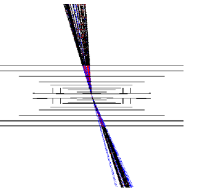
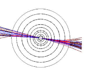
Figure 6.26: Two views of an event in the central detector, of the type $e^{+}e^{-}\to WW\nu\nu\to$ 4 jets $\nu\nu$, from a resonance with $M_{WW}$ = 2 TeV  [76]

A full spectrum, which contains contributions from all the channels $ZZ\to ZZ,ZZ\to WW,ZW\to ZW,WW\to ZZ$ and $WW\to WW$ is shown for 1.6 ab^-1 in Fig. 6.25, before and after detector smearing with parameters $\alpha_{5}$ = – 0.002, $\alpha_{4}$ = 0 [76].

Clearly heavy resonances in $WW$ scattering can be detected at CLIC. The signal is not heavily distorted by detector resolution and background. Depending on the mass and width of the signal, about a 1000 events per year could be fully reconstructed in the four-jet mode at CLIC. Good energy and track reconstruction will be important to remove backgrounds and reconstruct the resonance parameters (and hence the underlying model parameters) accurately.

The particular attractiveness of the study of this possible phenomenon at CLIC energies using the $e^{-}e^{-}$ channel is the availability of highly polarized electron beams, which either couple to $W^{-}$ (if the electron is left-handed ) or decouple (if right-handed). The ease with which the electron helicity can be inverted means that a real resonance effect in $W^{-}W^{-}$ interactions can trivially be separated from any obfuscating background.

6.4.2 Degenerate BESS Model

Strong symmetry-breaking models are based on low-energy effective Lagrangians, which provide a phenomenological description of the Goldstone boson dynamics. Possible new vector resonances produced by the strong interaction responsible for the electroweak symmetry-breaking can be introduced in this formalism as gauge bosons of a hidden symmetry. A description of a new triplet of vector resonances is obtained by considering an effective Lagrangian based on the symmetry $SU(2)_{L}\otimes SU(2)_{R}\otimes SU(2)_{\rm local}$ [77]. The new vector fields are a gauge triplet of the $SU(2)_{\rm local}$. They acquire mass as the $W^{\pm}$ and the $Z^{0}$ bosons. By enlarging the symmetry group of the model, additional vector and axial-vector resonances can be introduced.

The degenerate BESS model (D-BESS) [78] is a realization of dynamical electroweak symmetry-breaking with decoupling. The D-BESS model introduces two new triplets of gauge bosons, which are almost degenerate in mass: ($L^{\pm}$, $L_{3}$), ($R^{\pm}$, $R_{3}$). The extra parameters are a new gauge coupling constant $g^{\prime\prime}$ and a mass parameter $M$, related to the scale of the underlying symmetry-breaking sector. In the charged sector, the $R^{\pm}$ fields are not mixed and $M_{R^{\pm}}=M$, while $M_{{L}^{\pm}}\simeq M(1+x^{2})$ for small $x=g/g^{\prime\prime}$, with $g$ the usual $SU(2)_{W}$ gauge coupling constant. The $L_{3}$, $R_{3}$ masses are given by $M_{L_{3}}\simeq M\left(1+x^{2}\right),~{}~{}M_{R_{3}}\simeq M\left(1+x^{2}\tan^{2}\theta\right)$, where $\tan\theta=g^{\prime}/g$ and $g^{\prime}$ is the usual $U(1)_{Y}$ gauge coupling constant. These resonances are narrow, as seen in Fig. 6.17, and almost degenerate in mass with $\Gamma_{L_{3}}/M\simeq$ 0.068$x^{2}$ and $\Gamma_{R_{3}}/M\simeq$ 0.01$x^{2}$, while the neutral mass splitting is $\Delta M/M=(M_{L_{3}}-M_{R_{3}})/M\simeq\left(1-\tan^{2}\theta\right)x^{2}\simeq$ 0.70$x^{2}$.

This model respects the present bounds from electroweak precision data, since the $S,T,U$ (or $\epsilon_{1},\epsilon_{2},\epsilon_{3}$) parameters vanish at the leading order in the limit of large $M$, because of an additional custodial symmetry. Therefore, electroweak data set only loose bounds on the parameter space of the model. We have studied these bounds by considering the latest experimental values of the $\epsilon$ parameters coming from the high-energy data [18]: $\epsilon_{1}$ = (5.4 $\pm$ 1.0) $\times$ 10^-3, $\epsilon_{2}$ = (– 9.7 $\pm$ 1.2) $\times$ 10^-3, $\epsilon_{3}$ = (5.4 $\pm$ 0.9) $\times$ 10^-3. We have included radiative corrections, taken to be the same as in the SM, with the Higgs mass as a cut-off [78]. For $m_{t}$ = 175.3 GeV and $m_{H}$ = 1000 GeV, one has [79]: $\epsilon_{1}^{\rm rad}$ = 3.78 $\times$ 10^-3, $\epsilon_{2}^{\rm rad}$ = – 6.66 $\times$ 10^-3, $\epsilon_{3}^{\rm rad}$ = 6.65 $\times$ 10^-3. The 95% C.L. bounds on the parameters of the D-BESS model are shown in Fig. 6.27. Comparable bounds come from the direct search at the Tevatron [78].

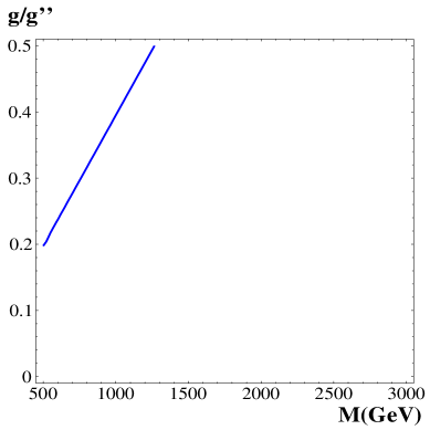
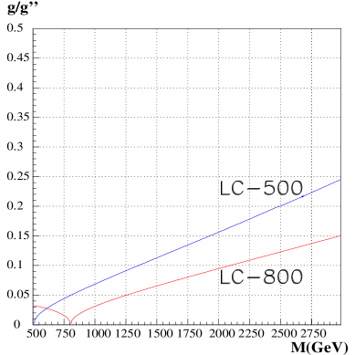
Figure 6.27: 95% C.L. contours in the plane $(M,~{}g/g^{\prime\prime})$ from the present $\epsilon$ measurements (left) and from measurements of $\sigma_{\mu^{+}\mu^{-}}$, $\sigma_{b\bar{b}}$, $A_{\rm FB}^{\mu\mu}$, $A_{\rm FB}^{bb}$ at $e^{+}e^{-}$ linear colliders with $\sqrt{s}$ = 500 (800) GeV and ${\cal{L}}$ = 1 ab^-1 (right). The allowed regions are below the curves.

The LHC can discover these new resonances, which are produced via $q\bar{q}$ annihilations, through their leptonic decay $q{\bar{q}^{\prime}}\to L^{\pm},W^{\pm}\to(e\nu_{e})\mu\nu_{\mu}$ and $q{\bar{q}}\to L_{3},R_{3},Z,\gamma\to(e^{+}e^{-})\mu^{+}\mu^{-}$.

The relevant observables are the dilepton transverse and invariant masses. The main backgrounds left in these channels after the lepton isolation cuts are the Drell–Yan processes with SM gauge bosons exchange in the electron and muon channels. A study has been performed using a parametric detector simulation [80]. Results are given in Table 6.10

Table 6.10: Sensitivity to production of the ${\rm L}_{3}$ and ${\rm R}_{3}$ D-BESS resonances at the LHC for ${\cal{L}}$ = 100 (500) fb^-1 with $M$ = 1.2 (3) TeV and accuracy on the mass splitting at CLIC for ${\cal{L}}$ = 1 ab^-1.

$g/g^{\prime\prime}$	$M$	$\Gamma_{{\rm L}_{3}}$	$\Gamma_{{\rm R}_{3}}$	$S/\sqrt{S+B}$	$\Delta M$
	(GeV)	(GeV)	(GeV)	LHC ($e+\mu$)	CLIC
1000	0.7	0.1	17.3
0.2	1000	2.8	0.4	44.7
0.1	2000	1.4	0.2	3.7
0.2	2000	5.6	0.8	8.8
0.1	3000	2.0	0.3	(3.4)	23.20 $\pm$ 0.06
0.2	3000	8.2	1.2	(6.6)	83.50 $\pm$ 0.02

for the combined electron and muon channels for ${\cal{L}}$ = 100 fb^-1, except for $M$ = 3 TeV where 500 fb^-1 are assumed. The discovery limit at the LHC, with ${\cal{L}}$ = 100 fb^-1, is $M\sim$ 2 TeV for $g/g^{\prime\prime}$ = 0.1. Beyond discovery, the possibility to disentangle the characteristic double-peak structure depends strongly on $g/g^{\prime\prime}$ and smoothly on the mass.

The LC can also probe this multi-TeV region through virtual effects in the cross sections for $e^{+}e^{-}\to{{\rm L}_{3}},{{\rm R}_{3}},Z,\gamma\to f\bar{f}$, at centre-of-mass energies below the resonances. Thanks to the presence of new spin-1 resonances, the annihilation channel in $f\bar{f}$ and $W^{+}W^{-}$ has a better sensitivity than the fusion channel. In the case of the D-BESS model, the ${\rm L}_{3}$ and ${\rm R}_{3}$ states are not strongly coupled to $W$ pairs, making the $f\bar{f}$ final states the most favourable channel for discovery. The analysis at $\sqrt{s}$ = 500 GeV and $\sqrt{s}$ = 800 GeV is based on $\sigma_{\mu^{+}\mu^{-}}$, $\sigma_{b\bar{b}}$, $A_{\rm FB}^{\mu\mu}$ and $A_{\rm FB}^{bb}$. We assume identification efficiencies of $\epsilon_{\mu}$ = 95% and $\epsilon_{b}$ = 60% and systematic uncertainties of $\Delta\epsilon_{\mu}/\epsilon_{\mu}$ = 0.5%, $\Delta\epsilon_{b}/\epsilon_{b}$ = 1%. The sensitivity contours obtained for ${\cal{L}}$ = 1 ab^-1 are shown in Fig. 6.27. The 3 TeV LC indirect reach is lower than that of the LHC or comparable to it. However, the QCD background rejection essential for the LHC sensitivity still needs to be validated using a full detector simulation and pile-up effects.

Assuming a resonant signal to be seen at the LHC or indirect evidence to be obtained at a lower-energy LC, CLIC could measure the width and mass of this state and also probe its almost degenerate structure [81]. This needs to be validated, taking the luminosity spectrum and accelerator-induced backgrounds into account. The ability to identify the model’s distinctive features has been studied using the production cross section and the flavour-dependent forward–backward asymmetries for different values of $g/g^{\prime\prime}$. The resulting distributions are shown in Fig. 6.28

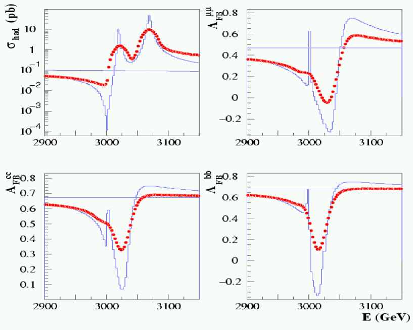
Figure 6.28: Hadronic cross section (upper left) and $\mu^{+}\mu^{-}$ (upper right), $c\bar{c}$ (lower left) and $b\bar{b}$ (lower right) forward–backward asymmetries at energies around 3 TeV. The continuous lines represent the predictions for the D-BESS model with $M$ = 3 TeV and $g/g^{\prime\prime}$ = 0.15, the flat lines the SM expectation, and the dots the observable D-BESS signal after accounting for the CLIC.02 luminosity spectrum.

for the case of the narrower CLIC.02 beam parameters [20]. A characteristic feature of the cross-Section distributions is the presence of a narrow dip, due to the interference of the ${\rm L}_{3}$, ${\rm R}_{3}$ resonances with the $\gamma$ and $Z^{0}$, and to cancellations of the ${\rm L}_{3}$, ${\rm R}_{3}$ contributions. Similar considerations hold for the asymmetries. In the case shown in Fig. 6.28, the effect is still visible after accounting for the luminosity spectrum. In this analysis, the beam-energy spread sets the main limit to the smallest mass splitting observable. With realistic assumptions and 1 ab^-1 of data, CLIC will be able to resolve the two narrow resonances for values of the coupling ratio $g/g^{\prime\prime}>$ 0.08, corresponding to a mass splitting $\Delta M$ = 13 GeV for $M$ = 3 TeV, and to determine $\Delta M$ with a statistical accuracy better than 100 MeV, as seen in Table 6.10.

6.5 Further Alternative Theories

There exist a plethora of other new phenomena that may appear at the TeV scale. In the following, we discuss briefly Little Higgs models, a possible fourth family of quarks and leptons, leptoquarks, excited leptons and leptons of finite size, and finally non-commutative field theories.

6.5.1 Heavy Gauge Bosons in Little Higgs Models

Within Little Higgs models [82], new heavy particles can be expected in the TeV range, such as a heavy top quark $T$ and new gauge bosons. The LHC is sensitive to these particles up to 2.5 TeV for the $T$ quark [83], but CLIC will produce these copiously, via associated ($W^{\prime},T$) or single ($Z^{\prime}$) production, allowing for a precise study of the properties of the particles.

The existence of the heavy $SU(2)$ gauge bosons $Z_{H}$ and $W_{H}$ is one of the main predictions of the Little Higgs models. The masses of $Z_{H}$ and $W_{H}$ should be within about a few TeV in order to solve the hierachy problem.

At an $e^{+}e^{-}$ linear collider, if the centre-of-mass (c.m.) energy can be set at the mass of the vector resonance, one is able to reach a substantial production cross section and perform precision studies of the properties of the particle. Above the resonance threshold, the dominant production for the heavy gauge bosons is through the $WW_{H}$ final state. Fixing $M_{W_{H}}$ = 1 TeV, we plot in Fig. 6.29 (solid curves) the total cross section for $WW_{H}$ production for $M_{W_{H}}$ = 1 and 2 TeV as a function of the c.m. energy.

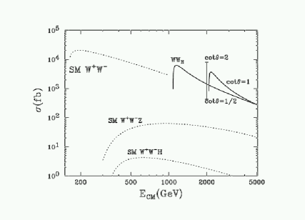
Figure 6.29: Total cross section for $e^{+}e^{-}\to WW_{H}$ production versus centre-of-mass energy $E_{c.m.}$ for $M_{W_{H}}$ = 1 and 2 TeV (solid curves). Both charge states $W^{\pm}~{}W_{H}^{\mp}$ have been included. Some relevant SM processes have also been included for comparison (dashed curves).

For a fixed value of $M_{W_{H}}$, the cross section scales as $\cot^{2}\theta$, and the changes for $\cot\theta$ = 1/2 and 2 are indicated by a vertical bar. For comparison, we also include some relevant SM processes of $W^{+}W^{-}$, $WWZ$, and $WWH$. We see that the signal cross section for the $WW_{H}$ final state is large and asymptotically decreases to the level of $W^{+}W^{-}$.

In Fig. 6.30, we show the total cross-Section versus $M_{W_{H}}$ at the CLIC energies, 3 and 5 TeV, for $\cot\theta~{}=~{}1$. The cross section grows when the mass increases because of the less and less severe propagator suppression $1/(s-M_{Z_{H}})^{2}$, until it is cut off by the threshold kinematics.

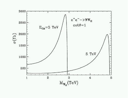
Figure 6.30: Total cross section for $e^{+}e^{-}\to WW_{H}$ production versus its mass $M_{W_{H}}$ at the CLIC energies $E_{c.m.}$ = 3 and 5 TeV. Both charge states $W^{\pm}~{}W_{H}^{\mp}$ have been included.

Generically, the mass and coupling of $W_{H}$ depend on $\cot\theta$, the mixing parameter between the SM and new gauge groups $SU_{L}(2)$ and $SU_{H}(2).$ Keeping the mass fixed at 1 TeV, we can explore the total cross section with respect to $\cot\theta$, as shown in Fig. 6.31.

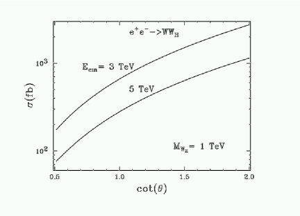
Figure 6.31: Total cross section for $e^{+}e^{-}\to WW_{H}$ production as a function of gauge coupling mixing parameter $\cot\theta$ for $M_{W_{H}}$ = 1 TeV

Once $W_{H}$ is produced, it can decay to SM particles, either fermion pairs or $WZ,\ WH$. The branching fractions are given with respect to the mixing parameter $\cot\theta$, as in Fig. 6.32. The decay channels to fermions are dominant, asymptotically 1/4 for the three generations of leptons or one generation of quarks, for most of the paramter space. For a value of $\cot\theta<$ 0.4, $W_{H}\to WH,WZ$ decay modes become more important, comparable to fermionic channels, as shown in Fig. 6.32. The production rate for the signal is still quite sizeable once above the kinematical threshold, and likely above the SM backgrounds.

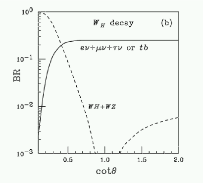
Figure 6.32: Branching fractions for $W_{H}$ decay to SM particles

In summary, once above the kinematical threshold, the heavy gauge boson production at the CLIC energies can be substantial. The threshold behaviour can determine its mass accurately, and the cross section rate will measure the coupling strength $\cot\theta$.

6.5.2 Fourth Family

The mass and mixing patterns of the fundamental fermions are among the most mysterious aspects of particle physics today. The number of fermion generations is not fixed by the SM. It is intriguing that flavour democracy may hint at the existence of a fourth SM family (see [84, 85] and references therein), and its possible existence is a fundamental question on which CLIC can cast new light. In order to avoid violation of partial-wave unitarity, the masses of new quarks and leptons should be smaller than about 1 TeV [86]. Therefore, CLIC with 1–3 TeV centre-of-mass energy will give the opportunity to measure the fourth-SM-family fermions and quarkonia in detail.

Fourth-family quarks, if they exist, will be copiously produced at the LHC [88, 87] if their masses are less than $1$ TeV. Therefore, any fourth-family quarks might be discovered at the LHC well before CLIC goes into operation. The same is true for pseudoscalar quarkonia ($\eta_{4}$) formed by the fourth-family quarks [89]. However, the observation of the fourth-family leptons at the LHC is problematic because of the large backgrounds from real $W$ and $Z$ boson production, both singly and in pairs, that hide these heavy lepton signals [90]. Lepton colliders will therefore be advantageous for the investigation of the fourth-SM-family leptons and vector ($\psi_{4}$) quarkonia. The potential of muon colliders was analysed in Ref. [91]. In this section we consider the production of the fourth-family fermions and quarkonia at CLIC, starting with pair production.

First we consider the $e^{+}e^{-}$ option of CLIC. The annihilation of $e^{+}e^{-}$ is a classic channel to produce and study new heavy fermions, because the cross sections are relatively large with respect to the backgrounds [90]. The obtained cross section values for pair production of the fourth-SM-family fermions with $m_{4}$ = 320 (640) GeV and the corresponding numbers of events per working year (10⁷ s) are given in Table 6.11 (Table 6.12). Event signatures are defined by the mass pattern of the fourth family and the 4 $\times$ 4 Cabibbo–Kobayashi–Maskawa (CKM) matrix. According to the scenario given in Ref. [92], the dominant decay modes are $u_{4}\to b$ $W^{-}$, $d_{4}\to t$ $W^{+}$, $l_{4}\to\nu_{\tau}W^{-}$ and $\nu_{4}\to\tau^{-}W^{+}$. The charged $l_{4}$ lepton will have a clear signature at CLIC. For example, if the produced $W^{\pm}$ bosons decay leptonically, one has two acoplanar opposite-charge leptons and large missing energy. Pair production of the neutral $\nu_{4}$ leptons will lead to a more complicated event topology. In this case, $\tau$ tagging will be helpful for the identification of the events. Indeed, the produced $\tau$ leptons will decay at a distance of 1–2 cm from the interaction point, which can easily be measured by a vertex detector. In addition, the polarization of electron and positron beams should help to experimentally determine the axial and vector neutral-current coupling constants of the fourth-family fermions.

Table 6.11: Cross sections and event numbers per year for pair production of the fourth-SM-family fermions with mass 320 GeV at CLIC ($\sqrt{s_{ee}}$ = 1 TeV, $L_{ee}$ = 2.7 $\times$ 10³⁴cm^-2s^-1 and $L_{\gamma\gamma}$ = 10³⁴cm^-2s^-1)

		$u_{4}\overline{u_{4}}$	$d_{4}\overline{d_{4}}$	$l_{4}\overline{l_{4}}$	$\nu_{4}\overline{\nu_{4}}$
$e^{+}e^{-}$ option	$\sigma$ (fb)	130	60	86	15
	Nev/year	35 000	16 000	23 000	4100
$\gamma\gamma$ option	$\sigma$ (fb)	34	2	58	–
	Nev/year	3400	200	5700	–

Table 6.12: Cross sections and event numbers per year for pair production of the fourth-SM-family fermions with mass 640 GeV at CLIC ($\sqrt{s_{ee}}$ = 3 TeV, $L_{ee}$ = 1 $\times$ 10³⁵cm^-2s^-1 and $L_{\gamma\gamma}$ = 3 $\times$ 10³⁴cm^-2s^-1)

		$u_{4}\overline{u_{4}}$	$d_{4}\overline{d_{4}}$	$l_{4}\overline{l_{4}}$	$\nu_{4}\overline{\nu_{4}}$
$e^{+}e^{-}$ option	$\sigma$ (fb)	16	8	10	2
	Nev/year	16 000	8000	10 000	2000
$\gamma\gamma$ option	$\sigma$ (fb)	27	2	46	–
	Nev/year	8100	600	14 000	–

Next we consider the $\gamma\gamma$ option [93, 94, 95] of CLIC. The fourth-SM-family quarks and charged leptons will also be copiously produced at $\gamma\gamma$ machines. For $\sqrt{s_{ee}}$ = 1 TeV (3 TeV), which corresponds to $\sqrt{s_{\gamma\gamma}}^{\max}$ = 0.83$\sqrt{s_{ee}}$ = 0.83 TeV (2.5 TeV), the obtained cross section values and number of events per year are presented in Table 6.11 (Table 6.12).

Next we discuss quarkonium production. The condition to form $(Q\overline{Q})$ quarkonia states with new heavy quarks is $m_{Q}\leq$ (125 GeV) $|V_{Qq}|^{-2/3}$, where $q=d,s,b$ for $Q=u_{4}$ and $q=u,c,t$ for $Q=d_{4}$ [96]. Unlike the $t$ quark, the fourth-family quarks will form quarkonia because $u_{4}$ and $d_{4}$ are almost degenerate and their decays are suppressed by small CKM mixings [97, 92, 84]. Below, we consider the resonance production of $\psi_{4}$ quarkonia at $e^{+}e^{-}$ and $\eta_{4}$ quarkonia at $\gamma\gamma$ options of CLIC.

Again we first consider the $e^{+}e^{-}$ option for CLIC. The cross section for the formation of the fourth-family quarkonium is given by the well-known relativistic Breit–Wigner equation

$$\sigma\left(e^{+}e^{-}\to\left(Q\overline{Q}\right)\right)=\frac{12\pi\left(s/M^{2}\right)\Gamma_{ee}\Gamma}{\left(s-M^{2}\right)^{2}+M^{2}\Gamma^{2}}\,,$$ (6.7)

where $M$ is the mass, $\Gamma_{ee}$ is the partial decay width to $e^{+}e^{-}$ and $\Gamma$ is the total decay width of the fourth-family quarkonium. Using corresponding formulae from [98] in the framework of the Coulomb potential model, we obtain decay widths for the main decay modes of $\psi_{4}(u_{4}\overline{u_{4}})$ and $\psi_{4}(d_{4}\overline{d_{4}})$, which are given in Table 6.13. One can see that the dominant decay mode for both $\psi_{4}(u_{4}\overline{u_{4}})$ and $\psi_{4}(d_{4}\overline{d_{4}})$ quarkonia is $\psi_{4}\to W^{+}W^{-}$. Other important decay modes are $\psi_{4}\to\gamma Z$ and $\psi_{4}\to\gamma H$.

Table 6.13: Decay widths for main decay modes of $\psi_{4}$ for $m_{H}$ = 150 GeV with $m_{\psi_{4}}\simeq$ 1 TeV

	($u_{4}\overline{u_{4}}$)	($d_{4}\overline{d_{4}}$)
$\Gamma(\psi_{4}\to\ell^{+}\ell^{-})$, 10-3 MeV	18.9	7.3
$\Gamma(\psi_{4}\to u\overline{u})$, 10-2 MeV	3.2	1.9
$\Gamma(\psi_{4}\to d\overline{d})$, 10-2 MeV	1.4	1.7
$\Gamma(\psi_{4}\to Z\gamma)$, 10-1 MeV	15	3.7
$\Gamma(\psi_{4}\to ZZ)$, 10-1 MeV	1.7	5.4
$\Gamma(\psi_{4}\to ZH)$, 10-1 MeV	1.7	5.5
$\Gamma(\psi_{4}\to\gamma H)$, 10-1 MeV	14.4	3.6
$\Gamma(\psi_{4}\to W^{+}W^{-})$, MeV	70.8	71.2

In order to estimate the number of produced quarkonium states, one should take into account the luminosity distribution at CLIC, which is influenced by the energy spread of electron and positron beams and beamstrahlung. In our calculations we use the GUINEA-PIG simulation code [99]. For illustration, we assume that $m_{\psi_{4}}\simeq$ 1 TeV. The estimated event numbers per year for $\psi_{4}$ production, as well as $\psi_{4}\to\gamma H$ and $\psi_{4}\to ZH$ decay channels are presented in Table 6.14. In numerical calculations we use $\Delta E/E$ = 10^-2 for the beam energy spread. If $\Delta E/E$ = 10^-3 can be achieved, the corresponding numbers will be enlarged by a factor of about 8. The $\gamma H$ decay mode of the $\psi_{4}(u_{4}\overline{u_{4}})$ quarkonium is promising for the study of Higgs boson properties, especially if the energy spread of electron and positron beams of about 10^-2  could be controlled to about 10^-3.

Table 6.14: The production event numbers per year for the fourth-SM-family $\psi_{4}$ quarkonia at a CLIC 1 TeV option with $m_{\psi_{4}}\simeq$ 1 TeV

	($u_{4}\overline{u_{4}}$)	($d_{4}\overline{d_{4}}$)
$e^{+}e^{-}\to\psi_{4}$	26 600	10 400
$e^{+}e^{-}\to\psi_{4}\to\gamma H$	510	50
$e^{+}e^{-}\to\psi_{4}\to ZH$	60	80

Finally, we discuss again the $\gamma\gamma$ collider. The pseudoscalar $\eta_{4}$ quarkonia formed by the fourth-SM-family quarks will be copiously produced at the LHC [87, 89]. Decay widths for the main decay modes of $\eta_{4}(u_{4}\overline{u_{4}})$ and $\eta_{4}(d_{4}\overline{d_{4}})$ are given in Table 6.15. From there, it is clear that the dominant decay mode is $\eta_{4}\to ZH$. One can estimate the $\gamma\gamma\to\eta_{4}$ production cross section by using the following relation [100]:

$$\sigma\approx 50\,{\rm fb}(1+\lambda_{1}\lambda_{2})\left(\frac{BR_{\gamma\gamma}}{4\times 10^{-3}}\right)\left(\frac{\Gamma_{\rm tot}}{1\,{\rm MeV}}\right)\left(\frac{200\,{\rm GeV}}{M_{\eta}}\right)^{3}\,,$$ (6.8)

where $BR_{\gamma\gamma}$ is the branching ratio of the $\eta_{4}\to\gamma\gamma$ decay mode, $\Gamma_{\rm tot}$ is the quarkonium total decay width and $\lambda_{1,2}$ are helicities of the initial photons. Assuming $\lambda_{1}\lambda_{2}$ = 1, we obtain total event numbers of $\eta_{4}$ produced per year as follows: 900 $\eta_{4}(u_{4}\overline{u_{4}})$ and 56 $\eta_{4}(d_{4}\overline{d_{4}})$. The corresponding numbers for $\eta_{4}\to ZH$ events are 610 and 38 events, respectively. The advantage of $\eta_{4}(u_{4}\overline{u_{4}})$ with respect to $\eta_{4}(d_{4}\overline{d_{4}})$ is obvious.

Table 6.15: Decay widths for main decay modes of $\eta_{4}$ for $m_{H}$ = 150 GeV with $m_{\eta_{4}}$ = 0.75 TeV

	($u_{4}\overline{u_{4}}$)	($d_{4}\overline{d_{4}}$)
$\Gamma(\eta_{4}\to\gamma\gamma)$, 10-3 MeV	19.5	1.06
$\Gamma(\eta_{4}\to Z\gamma)$, 10-3 MeV	4.6	3.7
$\Gamma(\eta_{4}\to ZZ)$, 10-1 MeV	2.2	2.8
$\Gamma(\eta_{4}\to gg)$, MeV	5.1	5.1
$\Gamma(\eta_{4}\to ZH)$, MeV	47.3	47.3
$\Gamma(\eta_{4}\to W^{+}W^{-})$, 10-2 MeV	5.7	5.7
$\Gamma(\eta_{4}\to t\overline{t})$, MeV	16.4	16.4
$\Gamma(\eta_{4}\to b\overline{b})$, 10-2 MeV	1.0	1.0

6.5.3 Leptoquarks

In the SM of electroweak and colour (QCD) interactions, quarks and leptons appear as formally independent components. However, the observed symmetry between the lepton and quark sectors in the SM could be interpreted as a hint for common underlying structures. If quarks and leptons are made of constituents there should appear, at the scale of constituent binding energies, new interactions among leptons and quarks. Leptoquarks (LQs) are exotic particles carrying both lepton number (L) and baryon number (B), which are colour (anti-)triplet, scalar or vector particles that appear naturally in various unifying theories beyond the SM. The interactions of LQs with the known particles are usually described by an effective Lagrangian that satisfies the requirement of baryon- and lepton-number conservation and respects the $SU(3)_{C}~{}\times~{}SU(2)_{W}~{}\times~{}U(1)_{Y}$ symmetry of the SM. There are nine scalar and nine vector leptoquark types in the Buchmüller–Rückl–Wyler (BRW) classification [101]. The scalar leptoquarks $(S,R)$ can be grouped into singlets $(S_{0},\widetilde{S}_{0}),$ doublets $(R_{1/2},\widetilde{R}_{1/2})$ and triplet $(S_{1}).$ Here, we assume only the mass, and the couplings to right-handed and/or left-handed leptons, denoted by $g_{\rm R}$ and $g_{\rm L}$, remain as free parameters [102]. From the BRW effective interaction Lagrangian [101] one can deduce the quantum numbers of scalar leptoquarks given in Table 6.5.3.

The leptoquarks are constrained by different experiments. Direct limits on leptoquark states are obtained from their production cross sections at different colliders, while indirect limits are calculated from the bounds on the leptoquark-induced four-fermion interactions in low-energy experiments. The mass limits for scalar leptoquarks from single and pair production, assuming electromagnetic coupling, are $M_{LQ}>$ 200 GeV [103] and $M_{LQ}>$ 225 GeV [104], respectively.

We have studied the potential of a CLIC-based $e\gamma$ collider to search for scalar leptoquarks, taking into account both direct and resolved photon processes. Scalar leptoquarks can be produced singly in $e\gamma$ collisions, via the process $e\gamma\to Sq$, where $S$ is any type of scalar leptoquark ($S$ or $R$). At $e\gamma$ colliders, with a photon beam produced by Compton backscattering [105], the maximum $e\gamma$ centre-of-mass energy is about 91% of the available energy. The projects of CLIC [106] colliders will be working at $\sqrt{s_{e^{+}e^{-}}}$ = 1 TeV to $\sqrt{s_{e^{+}e^{-}}}$ = 3 TeV. Corresponding high-energy photon beams can be obtained from the linacs with energies $\simeq$ 415 GeV and $\simeq$ 1245 GeV for CLIC at these energies.

We have implemented the interactions between scalar leptoquarks, leptons and quarks into the CompHEP program [55] with an internal photon spectrum. The main contribution to the total cross section comes from the $u$-channel quark-exchange diagram. For this reason, the total cross Sections for the production of scalar leptoquarks $R_{1/2}$(– 5/3), $S_{0}$(– 1/3) and $S_{1}$(– 1/3) practically coincide. This is also true for $R_{1/2}$(– 2/3), $\widetilde{R}_{1/2}$(– 2/3), $\widetilde{S}_{0}$(– 4/3) and $S_{1}$(– 4/3) type scalar leptoquarks.

The scalar leptoquarks can also be produced in $e\gamma$ collisions by resolved photon processes. In order to produce leptoquarks in the resonant channel through the quark component of the photon, we study the following signal for the scalar leptoquark $S$ (or $R$), $e+q_{\gamma}\to S\to e+q$. For CLIC-based $e\gamma$ colliders, the total cross section for resolved photon contribution is obtained by convoluting with the back-scattered laser photon distribution and photon structure function. The photon structure function consists of perturbative point-like parts and hadron-like parts $f_{q/\gamma}=f_{q/\gamma}^{\rm PL}+f_{q/\gamma}^{\rm HL}$ [107]. Since the contribution from the point-like part of the photon structure function was already taken into account in the calculation of the direct part, it was subtracted from $f_{q/\gamma}$ to avoid double counting at the leading-logarithmic level.

Both schemes can give comparable results for the production cross Section. Therefore, we add their contribution to form the signal. In this case, the total cross section for the production of scalar LQs is $\sigma=\sigma_{\rm D}+\sigma_{\rm R}$, where $\sigma_{\rm D}$ and $\sigma_{\rm R}$ denote the direct and resolved contributions to the total cross section, respectively. The total cross sections including both direct and resolved contributions are plotted in Fig. 6.33 for CLIC-based $e\gamma$ colliders with $\sqrt{s_{e^{+}e^{-}}}$ = 1 TeV. As can be seen from this figure, the contribution from the resolved process is dominant for small leptoquark masses and the direct contribution is effective for larger masses up to the kinematical limit. Depending on the centre-of-mass energy, the resolved contribution decreases sharply beyond a leptoquark mass value of about 70% of the collider energy. The direct contribution for a scalar leptoquark with $|Q|$ = 5/3 is larger than the scalar leptoquark with $|Q$— = 4/3. This can be explained by the quark-charge dependence of the cross sections for direct contributions. The coupling for the lepton–quark–leptoquark vertex can be parametrized as $g_{LQ}=\sqrt{4\pi\alpha\kappa}$, where $\kappa$ is a parameter.

Quantum numbers of scalar leptoquarks according to the BRW classification. The numbers in the parentheses in the last two columns denote the values for $g_{\rm L}=g_{\rm R}$.

Leptoquark	F	I	$Q_{\rm em}$	Decay	Coupling	$BR(S\to lq)$	$BR(S\to\nu q)$
				$e_{L}u_{L}$	$g_{0L}$
$S_{0}$	2	0	– 1/3	$e_{R}u_{R}$	$g_{0R}$	$\frac{g_{0L}^{2}+g_{0R}^{2}}{2g_{0L}^{2}+g_{0R}^{2}}\,(\frac{2}{3})$	$\frac{g_{0L}^{2}}{2g_{0L}^{2}+g_{0R}^{2}}(\frac{1}{3})$
				$\nu d_{L}$	$-g_{0L}$
$\widetilde{S}_{0}$	2	0	– 4/3	$e_{R}d_{R}$	$\widetilde{g}_{0R}$	1	0
		1	2/3	$\nu u_{L}$	$\sqrt{2}g_{1L}$	0 1
$S_{1}$	0	0	– 1/3	$\nu d_{L},e_{L}u_{L}$	$-g_{1L}$	1/2	1/2
		– 1	– 4/3	$e_{L}d_{L}$	$-\sqrt{2}g_{1L}$	1	0
		1/2	– 2/3	$\nu\overline{u}_{R}$	$g_{1/2L}$
		1/2	– 2/3	$e_{R}\overline{d}_{L}$	– $g_{1/2R}$	$\frac{g_{1/2R}^{2}}{g_{1/2R}^{2}+g_{1/2L}^{2}}(\frac{1}{2})$	$\frac{g_{1/2L}^{2}}{g_{1/2R}^{2}+g_{1/2L}^{2}}(\frac{1}{2})$
$R_{1/2}$	0
		– 1/2	– 5/3	$e_{L}\overline{u}_{R}$	$g_{1/2L}$	1	0
		– 1/2	– 5/3	$e_{R}\overline{u}_{L}$	$g_{1/2R}$
		1/2	1/3	$\nu\overline{d}_{R}$	$\widetilde{g}_{1/2L}$	0	1
$\widetilde{R}_{1/2}$	0
		– 1/2	– 2/3	$e_{L}\overline{d}_{R}$	$\widetilde{g}_{1/2L}$	1	0

The number of events and signal significance for $2j+e$ and $2j+\not\!p_{T}$ channels in scalar leptoquark decays. The lower and upper indices on scalar leptoquarks $S$ or $R$ denote weak isospin $I$ and $I_{3}$, respectively.

$\sqrt{s_{e^{+}e^{-}}}$ = 1 TeV	Number of events			$\frac{S}{\sqrt{B}}\,(e\gamma\to q\overline{q}e)$						$\frac{S}{\sqrt{B}}(e\gamma\to q\overline{q}^{\prime}\nu)$
$L_{\rm int}$ = 105 pb-1	$(\sigma_{\rm D}+\sigma_{\rm R})~{}\times~{}L_{\rm int}$
M${}_{\text{\rm LQ}}$(GeV)	$|Q|$ = 5/3	$|Q|$ = 4/3		$S_{0}$	$S_{1}^{0}$	$R_{1/2}^{-1/2}$	$R_{1/2}^{1/2}$	$\widetilde{R}_{1/2}^{-1/2},\widetilde{S}_{0},S_{1}^{-1}$		$S_{0}$	$S_{1}^{0}$	$R_{1/2}^{1/2}$
200	452407	210085		704	556	1113	258	517		89	135	63
300	247050	94763		401	304	608	117	233		49	74	28
400	157382	53386		255	194	387	66	131		31	47	16
500	107389	32904		174	132	264	40	81		21	32	10
600	76050	21310		123	94	187	26	52		15	23	6
700	54541	14335		88	67	134	18	35		11	16	4
800	38152	9782		62	47	94	12	24		7	11	–
900	6629	1660		11	8	16	2	4		1	2	–

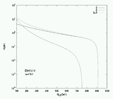
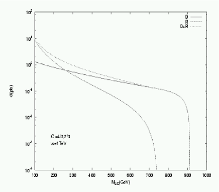
(a)                                                              (b)

Figure 6.33: The direct (D) and resolved (R) contributions to the cross section depending on scalar leptoquark mass $M_{LQ}$ at $\sqrt{s_{e^{+}e^{-}}}$ = 1 TeV with LQs charges a) $|Q|$ = 5/3 (1/3) and b) $|Q|$ = 4/3 (2/3).

When a scalar leptoquark is singly produced at an $e\gamma$ collider, the signal will be two jets and a charged lepton $2j+l$ ($S$ and $R$ leptoquarks), or two jets plus a neutrino $2j+\not\!p_{T}$ ($S$ leptoquarks). Since leptoquarks generate a peak in the invariant ($lj$) mass distribution, singly-produced leptoquarks are easy to detect up to mass values close to the kinematical limit. In the case of equal couplings $g_{\rm L}=g_{\rm R}$, the branching ratios for $S_{0}$ can be obtained as 2/3 for $LQ\to lq$ and 1/3 for $LQ\to\nu q$ channels.

In order to calculate the statistical significance $S/\sqrt{B}$ at each mass value of a scalar leptoquark and for each decay channel, we need to calculate also the relevant background cross sections. For the background processes $e\gamma\to W^{-}\nu$ and $e\gamma\to Ze$, we find the total cross sections 41.20 (49.48) pb and 2.36 (0.49) pb at $\sqrt{s_{e^{+}e^{-}}}$ = 1 (3) TeV, respectively. We multiply these cross sections with the branching ratios for the corresponding channels.

For a $e\gamma$ collider with centre-of-mass energy $\sqrt{s_{e^{+}e^{-}}}$ = 1 TeV and total luminosity $L$ = 10⁵ pb^-1, the scalar leptoquarks of types $S_{0},S_{1}^{0}$ and $R_{1/2}^{-1/2}$ can be produced up to mass $M_{LQ}\approx$ 900 GeV, and $R_{1/2}^{1/2},\widetilde{S}_{0},S_{1}^{-1},\widetilde{R}_{1/2}^{-1/2}$ up to $M_{LQ}\approx$ 850 GeV in the $2j+e$ channel. However, leptoquarks of types $S_{0},S_{1}^{0}$ can be produced up to $M_{LQ}\approx$ 850 GeV and $R_{1/2}^{1/2}$ up to $M_{LQ}\approx$ 650 GeV in the $2j+\not\!p_{T}$ channel. For an $e\gamma$ collider with $\sqrt{s_{e^{+}e^{-}}}$ = 3 TeV and total luminosity $L$ = 10⁵ pb^-1, the scalar leptoquarks of type $S_{0},S_{1}^{0},R_{1/2}^{-1/2}$ could be produced up to mass $M_{LQ}\approx$ 2600 GeV, types $\widetilde{R}_{1/2}^{-1/2},\widetilde{S}_{0},S_{1}^{-1}$ up to mass $M_{LQ}\approx$ 2500 GeV, type $R_{1/2}^{1/2}$ up to $M_{LQ}\approx$ 2100 GeV in the $2j+e$ channel; and scalar leptoquarks of type $R_{1/2}^{1/2}$ up to 700 GeV, $S_{0}$ up to 900 GeV and $S_{1}^{0}$ up to 1300 GeV in the $2j+\not\!p_{T}$ channel. The total number of signal events and statistical significance for these channels are given in Tables 6.5.3 and 6.5.3.

To conclude: scalar leptoquarks can be produced in large numbers at CLIC-based $e\gamma$ colliders. We have analysed the contributions from direct and resolved photon processes to the total cross section. We find that the latter contribution is important and cannot be ignored, especially for small leptoquark masses. Looking at the final-state particles and their signature in detectors, scalar leptoquarks of various types can be identified easily.

The same as Table 6.5.3, but for a CLIC-based $e\gamma$ collider with $\sqrt{s_{e^{+}e^{-}}}$ = 3 TeV

$\sqrt{s_{e^{+}e^{-}}}$ = 1 TeV	Number of events			$\frac{S}{\sqrt{B}}\,(e\gamma\to q\overline{q}e)$						$\frac{S}{\sqrt{B}}(e\gamma\to q\overline{q}^{\prime}\nu)$
$L_{\rm int}$ = 105 pb-1	$(\sigma_{\rm D}+\sigma_{\rm R})~{}\times~{}L_{\rm int}$
M${}_{\text{\rm LQ}}$(GeV)	$|Q|$ = 5/3	$|Q|$ = 4/3		$S_{0}$	$S_{1}^{0}$	$R_{1/2}^{-1/2}$	$R_{1/2}^{1/2}$	$\widetilde{R}_{1/2}^{-1/2},\widetilde{S}_{0},S_{1}^{-1}$		$S_{0}$	$S_{1}^{0}$	$R_{1/2}^{1/2}$
300	181523	124657		648	491	981	337	674		33	49	34
500	73182	35515		261	198	396	99	197		13	20	10
700	43722	18168		156	118	236	49	98		8	12	5
900	30084	11135		107	81	163	30	60		5	8	3
1100	22141	7513		79	60	120	20	41		4	6	–
1300	16929	5335		60	46	92	14	29		–	5	–
1500	13251	3906		47	36	72	11	21		–	4	–
1700	10520	2922		38	28	57	8	16		–	–	–
1900	8406	2225		30	23	45	6	12		–	–	–
2100	6705	1728		24	18	36	5	9		–	–	–
2300	5340	1377		19	14	29	4	7		–	–	–
2500	3842	975		14	10	21	–	5		–	–	–
2700	824	206		3	2	4	–	1		–	–	–

6.5.4 Lepton-Size Measurements

High-energy $e^{+}e^{-}$ scattering can also be used to study whether the leptons have a finite size. Similar studies have been made in the past, for example at LEP [108]. A model inspired by string theory, which can lead to elastic ministrings, with finite size (dubbed Nylons), has been proposed in Ref. [109].

In the presence of structure, annihilations to fermions $f$ will be modified to become $\frac{d\sigma}{dQ^{2}}=(\frac{d\sigma}{dQ^{2}})_{\rm SM}F_{e}^{2}(Q^{2})F_{f}^{2}(Q^{2})$, with $F(Q^{2})=1+\frac{1}{6}Q^{2}R^{2}$, where $R$ is an effective fermion radius. The current best limit on the radius $R_{e}$ of the electron comes from LEP, and is $R_{e}<$ 2.8 $\times$ 10^-17 cm (95 C.L.). For CLIC, the results for $ee\to ee$, under the assumption that the $t$ channel dominates, for an angular cut on the scattered electrons of $|\cos\theta|<$ 0.9, and for a luminosity of 500 fb^-1, are given in Table 6.16. We see that a 5-TeV machine will probe structures of dimensions a factor of 10 smaller than in the present results from LEP [108].

Table 6.16: Bounds on the possible electron radius $R_{e}$ obtainable with CLIC operating at various centre-of-mass energies

Radius (cm)		$\sqrt{s}$ (TeV)
3.0 $\times$ 10-18		1
1.2 $\times$ 10-18		3
0.9 $\times$ 10-18		5

6.5.5 Excited Electrons

The replication of three fermionic generations of known quarks and leptons suggest, the possibility that they are composite structures made up of more fundamental constituents. The existence of such quark and lepton substructure leads one to expect a rich spectrum of new particles with unusual quantum numbers. A possible signal of excited states of quarks and leptons [110] as predicted by composite models [111] would supply convincing evidence for a new substructure of matter. All composite models of fermions have an underlying substructure that may be characterized by a scale $\Lambda$. The absence of electron and muon electric dipole moments implies that the excited leptons must have specific chiral properties. A right-handed excited lepton should couple only to the left-handed component of the corresponding lepton. Excited leptons may be classified by $SU(2)~{}\times~{}U(1)$ quantum numbers, and they are assumed to be both left- and right-handed weak isodoublets. In the effective Lagrangian of [110], the parameters $f$ and $f^{\prime}$ associated with the gauge groups SU(2) and U(1) depend on compositeness dynamics and describe the effective changes from the SM coupling constants $g$ and $g^{\prime}$.

Experimental lower limits for the excited electron mass are given as $m_{e^{\star}}>$ 200 GeV in [112], and $m_{e^{\star}}>$ 306 GeV in [113]. The higher limits are derived from indirect effects due to $e^{\star}$ exchange in the $t$ channel, and depend on a transition magnetic coupling between $e$ and $e^{\star}$. Relatively small limits ($m_{\mu^{\star},\tau^{\star}}>$ 94.2 GeV) for excited muon ($\mu^{\star}$) and excited tau ($\tau^{\star}$) are given by the L3 experiment at LEP [114].

In this work, resonant production of an excited electron in the $s$ channel and its subsequent decay modes $e^{\star}\to e\gamma$, $e^{\star}\to\nu W$, $e^{\star}\to eZ$ are considered. In addition, we include the contributions coming from the excited electron in the $t$ channel. The production cross section and decays of excited electrons are calculated using the effective Lagrangian of [110], which depends on a compositeness scale $\Lambda$ and on free parameters $f$ and $f^{\prime}$. We have implemented the interaction vertices into CompHEP [55] for the excited electron interactions with leptons and gauge bosons. We choose either $f=f^{\prime}$ or $f=-f^{\prime}$ in our calculations in order to reduce the number of free parameters. For the case $f=f^{\prime}$ ($f=-f^{\prime}$) the coupling of the photon to excited neutrinos (electrons) vanishes.

When produced, an excited electron decays predominantly into a $W$ boson and a neutrino, and the branching ratios are insensitive to the excited electron mass when it is high with respect to $m_{W}$ or $m_{Z}$. We obtain the limiting values for the branching ratios at large $m_{e^{\star}}$ as 0.28, 0.60 and 0.11 for the coupling $f=f^{\prime}$ = 1, in the photon, $W$ and $Z$ channels, respectively. In the case $f=-f^{\prime}$ = – 1, the branching ratio for the $W$ channel does not change, whilst it increases to 0.39 for the $Z$ channel. Taking $f=-f^{\prime}$ = 1 and $\Lambda$ = 1 TeV, we find the total decay width of an excited electron to be 0.83 GeV and 6.9 GeV for $m_{e^{\star}}$ = 500 GeV and $m_{e^{\star}}$ = 1000 GeV, respectively.

Excited electrons can be produced directly via the subprocess $e\gamma\to e^{\star}\to lV$ ($V=\gamma,Z,W$) and indirectly via a $t$-channel exchange diagram [115]. The production cross section of excited electrons in three modes, taking $f=f^{\prime}$ = 1 and $\Lambda=m_{e^{\star}}$, are given in Table 6.5.5 for CLIC-based $e\gamma$ colliders at the centre-of-mass energy $\sqrt{s_{e^{+}e^{-}}}$ = 1 TeV ($\sqrt{s_{e^{+}e^{-}}}$ = 3 TeV). The following information can be read off Table 6.5.5 the following information: the $W$ channel gives higher cross sections than the others, but there is an ambiguity with the neutrino in this final state. Therefore, the photon channel gives a more promising result, because of its simple kinematics. The cross sections and the numbers of signal events are shown in Table 6.5.5. For the signal and background processes we apply a cut $p^{e,\gamma}_{T}>$ 10 GeV for experimental identification of final-state particles. The backgrounds to the $W$ and $Z$ decay channels in the hadronic final states are fairly large. The backgrounds to the photonic final states are relatively small with respect to the $W$ and $Z$ channels.

For the signal process $e\gamma\to e^{\star}\to e\gamma$, the transverse momentum $p_{T}$ distribution of the photon or electron is peaked around the half of the mass value of the excited electron, as seen in Fig. 6.34. For the process $e\gamma\to e^{\star}\to\nu W\,(eZ)$, the $p_{T}$ distribution of the $W$ boson (electron) shows a peak around ${m_{e^{\star}}/2}-{m^{2}_{V}/2m_{e^{\star}}}$, where $m_{V}$ denotes the $W$ boson (or $Z$ boson) mass.

In order to estimate the number of events for the signal and background in a chosen $p_{T}$ window, we integrate the transverse momentum distribution around the half the mass of each excited electron ($m_{e^{\star}}/2-m_{V}^{2}/2m_{e^{\star}}$) in an interval of the transverse momentum resolution $\Delta p_{T}$. Here $\Delta p_{T}$ is approximated as $\approx 10$ GeV for $m_{e^{\star}}~{}=~{}500$ GeV and $\approx 15$ GeV for $m_{e^{\star}}=750$ GeV, for a generic detector. In order to calculate the significance of the signal, we use integrated luminosities for CLIC-based $e\gamma$ colliders of $L$ = 10⁵ pb^-1. In order to see the potential of CLIC-based $e\gamma$ colliders to search for an excited electron, we define the statistical significance $S/\sqrt{B}$, where $S$ and $B$ are the total number of events for signal and background inside the chosen $p_{T}$ window, respectively. We calculate the value of $S/\sqrt{B}$ for different couplings, assuming $f=f^{\prime}$ and requiring the condition $S/\sqrt{B}>$ 5 for the signal to be observable. We find from Table 6.5.5 that excited electrons can be observed down to couplings $f\simeq$ 0.05 and $f\simeq$ 0.1 at CLIC-based $e\gamma$ colliders with $\sqrt{s_{e^{+}e^{-}}}$ = 1 TeV and $\sqrt{s_{e^{+}e^{-}}}$ = 3 TeV, respectively.

In this study, we have assumed that the excited electrons interact with the SM particles through the effective Lagrangian [110]. This may be a conservative assumption, because it is possible for excited fermions to couple to ordinary quarks and leptons via contact interactions originating from the strong constituent dynamics. In this case, the decay widths can be enhanced [116].

To conclude: we have presented results for excited electron production with subsequent decays into three channels. The excited electrons can be produced at CLIC-based $e\gamma$ colliders up to the kinematical limit in each channel, due to the nearly flat photon energy spectrum. We find that an excited electron with mass 500 (750) GeV can be probed down to the coupling $f=f^{\prime}\simeq$ 0.05 at $\sqrt{s_{e^{+}e^{-}}}$ = 1 TeV. At a CLIC-based $e\gamma$ collider with $\sqrt{s_{e^{+}e^{-}}}$ = 3 TeV the excited electron can be probed down with couplings as low as $f=f^{\prime}\simeq$ 0.1.

The total cross sections of signal and background inside the chosen bin and the statistical significance ($S/\sqrt{B}$) values for different $f=f^{\prime}$ for $m_{e^{\star}}$ = 750 GeV at $\sqrt{s_{e^{+}e^{-}}}$ = 1 TeV ($\sqrt{s_{e^{+}e^{-}}}$ = 3 TeV) with $L$ = 10⁵ pb^-1.

		$e\gamma\to e\gamma$			$e\gamma\to\nu W$			$e\gamma\to eZ$
$f=f^{\prime}$		$\sigma_{\rm tot}$ (pb)	$S/\sqrt{B}$		$\sigma_{\rm tot}$ (pb)	$S/\sqrt{B}$		$\sigma_{\rm tot}$ (pb)	$S/\sqrt{B}$
1.00		24.70 (4.30)	1892.4 (963.1)		80.10 (53.40)	1869.3 (211.3)		8.90 (1.51)	1905.5 (705.4)
0.50		11.30 (1.80)	963.1 (183.8)		51.40 (50.00)	466.5 (51.9)		3.40 (0.53)	694.4 (131.2)
0.10		7.04 (1.20)	18.9 (6.1)		42.13 (48.94)	13.2 (0.7)		1.60 (0.32)	24.3 (4.1)
0.05		6.87 (1.18)	0.7 (0.8)		41.88	1.1		1.52	3.9

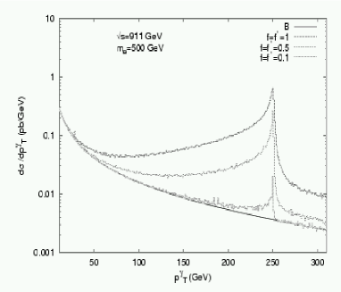
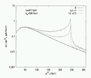
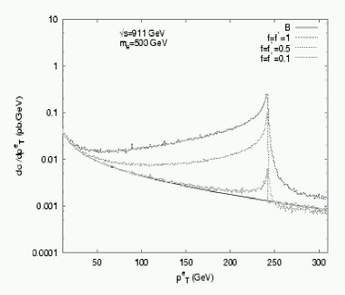
Figure 6.34: Transverse momentum distribution of the photon, $W$ boson and electron from excited electron production processes at a CLIC-based $e\gamma$ collider with $\sqrt{s_{e\gamma}^{\rm max}}$ = 911 GeV for different couplings $f=f^{\prime}$ and $m_{e^{\star}}$ = 500 GeV

6.5.6 Non-Commutative Theories

Recent theoretical studies have demonstrated that non-commutative (NC) quantum field theories appear naturally in the context of string theory in the presence of background fields [117]. In this case, the usual space-time coordinates no longer commute, and instead obey the relation

$$[\hat{x}_{\mu},\hat{x}_{\nu}]=i\theta_{\mu\nu}\,,$$ (6.9)

where the $\theta_{\mu\nu}$ are a constant, frame-independent set of six dimensionful parameters [118]. The $\theta_{\mu\nu}$ may be separated into two classes: (i) space–space non-commutativity with $\theta_{ij}=c^{B}_{ij}/\Lambda_{\rm NC}^{2}$, and (ii) space-time non-commutativity with $\theta_{0i}=c^{E}_{0i}/\Lambda_{\rm NC}^{2}$. The quantities $\hat{c}_{E,B}$ are two, fixed, frame-independent unit vectors associated with the NC scale $\Lambda_{\rm NC}$. The NC scale $\Lambda_{\rm NC}$ is most likely to be near the string or Planck scale, which could be as low as a TeV; it characterizes the threshold where NC effects become apparent. Since the two vectors $\hat{c}_{E,B}$ are frame-independent, they correspond to preferred directions in space, related to the directions of the background fields. Thus, NC theories violate Lorentz invariance, and upper limits on such effects provide model-dependent constraints on the NC scale [118, 119]. Since experimental probes of NC theories are sensitive to the directions of $\hat{c}_{E,B}$, the experiments must employ astronomical coordinate systems and time-stamp their data so that the rotation of the Earth or the Earth’s motion around the Sun, for example, does not wash out or dilute the effect through time-averaging. Note that momenta still commute in the usual way and hence energy and momentum remain conserved quantities, as does CPT.

It is possible to construct non-commutative analogues of conventional field theories following two approaches: Weyl–Moyal (WM) [118] or Seiberg–Witten (SW) [117], both of which have their own advantages and disadvantages. In the SW approach, the field theory is expanded in a power series in $\theta$, which then produces an infinite tower of additional operators. At any fixed order in $\theta$ the theory can be shown to be non-renormalizable [120]. The SW construction can, however, be applied to any gauge theory with arbitrary matter representations. In the WM approach, only $U(N)$ gauge theories are found to be closed under the group algebra, and the matter content is restricted to the (anti-)fundamental and adjoint representations. However, these theories are at least one-loop renormalizable, and appear to remain so even when spontaneously broken [121]. These distinctive properties of NC gauge theories render it difficult to construct a satisfactory non-commutative version of the SM [122].

However, a NC version of QED is a well-defined theory in the WM approach, and its implications for very-high-energy $e^{+}e^{-}$ colliders may be explored. This version of NCQED differs from ordinary QED in several ways: (i) the ordering of products of fields must be preserved through the introduction of the star product [118], which absorbs the effect of the commutation relation via a series of Fourier transforms; (ii) all vertices pick up a Lorentz-violating phase factor that is dependent on the momenta flowing through the vertex; (iii) NCQED takes on a non-Abelian nature in that trilinear and quartic photon couplings are generated; and (iv) only the charges $Q$ = 0, $\pm$ 1 are allowed by gauge invariance. We note that propagators, however, are not modified since quadratic forms remain unchanged when one introduces the star product.

NCQED provides a testing ground for the basic ideas behind NC quantum field theory, and produces striking signatures in QED processes at CLIC. The NC modifications to pair annihilation, Bhabha, Møller, and Compton scattering, as well as $\gamma\gamma\to\gamma\gamma,e^{+}e^{-}$ have been examined by a number of authors [123]. Some of these processes receive new diagrammatic contributions due to the non-Abelian couplings, and all of them acquire a phase dependence due to the relative interference of the vertex kinematic phases. The lowest-order NC contribution to these processes occurs via dimension-8 operators whose scale is set by $\Lambda_{\rm NC}$. The most striking result is that an azimuthal-angle, $\phi$, dependence is induced in $2\to 2$ scattering processes, since there exist the NC-preferred space-time directions, providing a unique signature of the Lorentz violation inherent in these theories.

Very-high-energy $e^{+}e^{-}$ colliders such as CLIC will allow us to probe values of $\Lambda_{\rm NC}$ up to several TeV provided sufficient luminosity, $\sim$ 1 ab^-1, is available [124]. To demonstrate this claim, we examine the case of pair annihilation, taking the incoming $e^{-}$ direction to be along the $z$-axis. In addition to the new phases that enter the $t$- and $u$-channel amplitudes, there is now an additional $s$-channel photon exchange graph involving the NC-generated three-photon vertex. The resulting azimuthal dependence and $\cos\theta$ distribution are shown in Fig. 6.35 for the illustrative case $c_{02}$ = 1. Writing $c_{01}=\cos\alpha$, $c_{02}=\sin\alpha\cos\beta$, and $c_{03}=\sin\alpha\sin\beta$, Fig. 6.36 displays the reach for $\Lambda_{\rm NC}$ for CLIC energies for several values of $\alpha$.

The 95% C.L. search reaches for the NC scale in a variety of processes are summarized in Table 6.17 for both $\sqrt{s}$ = 500 GeV and CLIC energies. We see that these machines have a reasonable sensitivity to NC effects and provide a good probe of such theories. It turns out that Møller scattering, while sensitive only to space/space non-commutativity, is a particularly promising process for experimental investigation: once the non-commutative Feynman rules are written down, we can interpret precise measurements of the Møller scattering cross-Section. It may be the interaction of choice for a possible observation of this new effect.

     

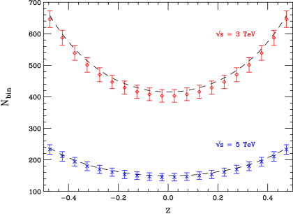
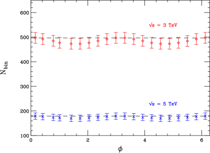
Figure 6.35: Shifts in the $z=\cos\theta$ and $\phi$ distributions for the process $e^{+}e^{-}\to\gamma\gamma$ at a 3 or 5 TeV CLIC, assuming an integrated luminosity of 1 ab^-1. The dashed curves show the SM expectations while the ‘data’ assume $c_{02}$ = 1 and $\Lambda_{\rm NC}=\sqrt{s}$. A cut of $|z|<$ 0.5 has been applied in the $\phi$ distribution.

     

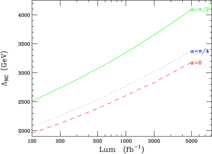
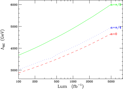
Figure 6.36: Reach for $\Lambda_{\rm NC}$ at a 3 TeV (left) or a 5 TeV (right) CLIC as a function of the integrated luminosity for the process $e^{+}e^{-}\to\gamma\gamma$ following the notation discussed in the text

Table 6.17: Summary of the 95% C.L. search limits on the NC scale $\Lambda_{\rm NC}$ from the various processes considered above at a 500 GeV $e^{+}e^{-}$ linear collider with an integrated luminosity of 500 fb^-1 or at a 3 or 5 TeV CLIC with an integrated luminosity of 1 ab^-1. The sensitivities are from the first two papers in Ref. [123]. The $\gamma\gamma\to e^{+}e^{-}$ and $\gamma e\to\gamma e$ analyses of Godfrey and Doncheski include an overall 2% systematic error not included by Hewett, Petriello and Rizzo.

Process		Structure probed	$\sqrt{s}$ = 500 GeV	$\sqrt{s}$ = 3 TeV	$\sqrt{s}$ = 5 TeV
$e^{+}e^{-}\to\gamma\gamma$		Space-time	740–840 GeV	2.5–3.5 TeV	3.8–5.0 TeV
Møller scattering		Space–space	1700 GeV	5.9 TeV	8.5 TeV
Bhabha scattering		Space-time	1050 GeV	4.5–5.0 TeV	6.6–7.2 TeV
$\gamma\gamma\to\gamma\gamma$		Space-time	700–800 GeV
		Space–space	500 GeV
$\gamma\gamma\to e^{+}e^{-}$		Space-time	220–260 GeV	1.1–1.3 TeV	1.8–2.1 TeV
$\gamma e\to\gamma e$		Space-time	540–600 GeV	3.1–3.4 TeV	4.8–5.8 TeV
		Space–space	700–720 GeV	4.0–4.2 TeV	6.3–6.5 TeV

6.6 Summary

A summary of the reach for exotic physics at CLIC, assuming a centre-of-mass energy of 5 TeV and an integrated luminosity of 5 ab^-1, is given in Table 6.18.

Table 6.18: Summary of the physics reach of CLIC for various examples of exotic new physics, assuming $\sqrt{s}$ = 5 TeV and an integrated luminosity of 5 ab^-1

$Z^{\prime}$ (direct)		5 TeV
$Z^{\prime}$ (indirect)		30 TeV
$l^{*},q^{*}$		5 TeV
TGC (95%)		0.00008
$\Lambda$ compos.		400 TeV
$W_{L}W_{L}$		$>$ 5 TeV
ED (ADD)		30 TeV ($e^{+}e^{-}$)
		55 TeV ($\gamma\gamma$)
ED (RS)		18 TeV ($c$ = 0.2)
ED (TeV-1)		80 TeV
Resonances		$\delta M/M,\delta\Gamma/\Gamma\sim$ 10-3
Black holes		5 TeV

As we have shown in this chapter, the particular characteristics of CLIC, such as larger beamstrahlung and $\gamma\gamma$ backgrounds than a lower-energy LC, are not in general obstacles to full exploitation of CLIC’s higher centre-of-mass energy. If the new physics is within CLIC’s kinematic reach, CLIC will find it.

In many cases, CLIC will be able to explore in detail and unravel hints of new physics that might be found at the LHC. In other cases, CLIC can reach even far beyond the LHC, thanks to its relatively clean experimental conditions and its democratic production of new weakly-interacting particles.

Chapter 7 QCD

7.1 Introduction

Strong-interaction measurements at a multi-TeV $e^{+}e^{-}$ collider such as CLIC will constitute an important part of its physics programme. CLIC will provide unique tests of QCD at high energy scales in a relatively clean experimental and theoretical environment. Examples of general QCD measurements that can be made include the fragmentation and hadronization of partons at high energies and a precise extraction of $\alpha_{s}$ through multijet rates and event-shape variables, for example. For a TeV-class linear collider, a precision in $\alpha_{s}$ of the order of 1% may be achievable if the relevant perturbative QCD calculations become available with sufficiently high precision [2]. Also, virtual $\gamma\gamma$ interactions can be studied at an $e^{+}e^{-}$ collider, which will help the understanding of low-$x$ data at hadron colliders. A dedicated $\gamma\gamma$ collider interaction region would allow further detailed measurements of the enigmatic photon structure.

In this chapter, the following items, essentially in the category of two-photon physics, have been worked out in more detail:

• Measurement of the total $\gamma\gamma$ cross section

• Measurement of the photon structure

• Measurement of BFKL dynamics

At lower-energy $e^{+}e^{-}$ colliders, two-photon interactions have traditionally been studied using bremsstrahlung photons from the electron beams [3]. Similar processes, together with reactions induced by beamstrahlung photons, will also occur at a future high-energy $e^{+}e^{-}$ collider such as CLIC, and will allow a rich two-photon physics programme. The energy spectra of the photons emitted in these processes are, however, peaked at rather low energies.

Since the colliding beams are used only once at linear colliders, other operation modes become possible, such as a photon ($\gamma\gamma$) collider (PC) [4, 5]. At a PC, the electron and positron beams of a linear collider are converted into photon beams via Compton laser backscattering. This option has been discussed for CLIC in chapter 2. The advantage of the photon spectrum from laser backscattering is that it peaks at high energy values, typically $\sim$ 80% of the initial electron energy, with a relatively narrow width of approximately 10%. Thus, a PC offers the exciting possibility of studying two-photon interactions at the highest possible energies with high luminosity.

Finally, we note in passing that, since the overlaid $\gamma\gamma$ collisions form the most important background at CLIC, a good knowledge and understanding of two-photon processes will be essential for controlling these background contributions to other processes.

7.2 Total Cross Section

A key example for the study of the properties of the photon is the total $\gamma\gamma$cross section, which is not yet understood from first principles. The nature of the photon itself is known to be rather complex. A high-energy photon can fluctuate into a fermion pair or even into a hadronic bound state, i.e. a vector meson with the same quantum numbers as the photon, $J^{PC}$ = 1^–. These quantum fluctuations lead to the so-called hadronic structure of the photon.

The data from LEP [11, 12, 13, 14] show that the total $\gamma\gamma$cross section rises with energy. Such a rise was observed previously in $pp$ collisions, but, intriguingly, the rise in $\gamma\gamma$ collisions seems to be steeper. Figure 7.1 shows the data [11, 12, 13, 14] together with predictions of various models.

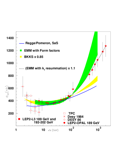
Figure 7.1: The total $\gamma\gamma$cross section as function of the collision energy, compared with model calculations: a band of predictions in the BKKS model, whose upper and lower limits correspond to different photon densities [6]; a proton-like model (solid line  [7, 8, 9]); an eikonal minijet model (EMM) band for the total and inelastic cross sections, with different photon densities and different minimum jet transverse momenta [10]). The proton-like and BKKS models have been normalized to the data, in order to show the energy dependence of the cross section.

As seen in Fig. 7.1, models differ in their predictions for the total $\gamma\gamma$ cross section at CLIC energies. The wide band is obtained using the eikonal minijet model (EMM), the thinner one using a model due to BKKS [6], and the full curve is an early prediction by Schuler and Sjöstrand [8] using a Regge–Pomeron fit. The EMM, which embeds QCD minijet cross sections in an eikonal formalism [15, 16], can describe the rise observed in present LEP data quite well, apart from a 10% normalization uncertainty. The predictions for $\gamma\gamma$ interactions are obtained with a parameter set extrapolated from similar fits to the photoproduction cross section at HERA. The tuned parameters include the different parton densities, minimum minijet transverse momenta, the soft cross section and a model for the transverse momentum distribution of partons in the photon. It should be noted, however, that the EMM, with a form-factor model for the parton transverse momentum distribution and the same set of parameters, does not reproduce at all the early rise seen in proton–proton scattering, unless higher-order effects due to soft gluon emission are included [17]. Although at present energies the EMM without soft gluons can describe the $\gamma\gamma$ data well, within the experimental errors, reliable predictions at higher energies, like those at CLIC, will require the proper inclusion of such higher-order contributions. The figure shows the effect of applying one particular realization of this idea [17] to the $\gamma\gamma$ case. Predictions for CLIC energies, based on soft gluon resummation and after fixing the normalization, are shown for a particular chosen set of parameters.

Clearly, new measurements at a higher-energy linear collider will be indispensable for establishing whether the photon cross section indeed rises faster than, for instance, the $pp$ data. A detailed comparison of the predictions of the different models for $\gamma\gamma$ cross sections reveals that, in order to distinguish between them, the cross sections should be determined to a precision of better than about 10% [10] at a future 0.5–1 TeV $e^{+}e^{-}$ collider [2], though the differences between models get larger at larger energy. This precision will however be difficult to achieve at an $e^{+}e^{-}$ collider, since the variable $\sqrt{s}_{\gamma\gamma}$needs to be reconstructed from the visible hadronic final state in the detector, which is a problem already at LEP. For example, the hadronic final state in the pseudorapidity $\eta=\ln\tan\theta$/2 extends over the range – 9 $<\eta<$ 9 at 3 TeV, while the detector covers roughly the region – 3 $<\eta<$ 3.

As already mentioned, at a $\gamma\gamma$ collider the photon beam energy can be tuned with a spread of less than 10%, so that measurements of $\sigma_{\gamma\gamma}^{\rm tot}$can be made at a number of ‘fixed’ energies, e.g. in the range 0.5 $<\sqrt{s_{\gamma\gamma}}<$ 2.5 TeV, as shown in Fig. 7.1. A detailed study reveals that the absolute precision with which these cross sections can be measured in the TeV region ranges from 8% to 15%, where the largest contributions to the errors are due to the modelling of the diffractive component of the cross section, the choice of the Monte Carlo model used to correct for the event selection cuts, the knowledge of the absolute luminosity and the shape of the luminosity spectrum. It will be necessary to constrain the diffractive component using high-energy two-photon data. A technique to measure diffractive contributions separately, modelled on the rapidity gap methods used at HERA, has been proposed in Ref. [18]. The potential measurements that can be made at CLIC are shown in Fig. 7.1 with 15% total errors.

Finally, we can use the above model predictions to update the calculation of the number of hadronic events per bunch crossing, which is expected to be significant at a high-energy $e^{+}e^{-}$ collider such as CLIC. However, in this case, it is necessary to add the effect of the beamstrahlung photons as well. We do this for CLIC using the spectra of beamstrahlung photons provided in Ref. [19]. For the design parameters considered, the two-photon luminosities per bunch crossing, corresponding to one or both photons being due to bremsstrahlung, are ${\cal L}_{eg}^{\gamma\gamma}$ = 5.3589 $\times$ 10³⁴ m^-2 or ${\cal L}_{ee}^{\gamma\gamma}$ = 6.4852 $\times$ 10³⁴ m^-2, respectively, whereas that due to beamstrahlung photons alone is ${\cal L}_{gg}^{\gamma\gamma}$ = 4.9534 $\times$ 10³⁴ m^-2. The numbers of hadronic events expected per bunch crossing, using these effective two-photon luminosities per bunch crossing, are shown in Table 7.1, for three different values of the lower limit on $s_{\gamma\gamma}$, instead of the fixed value of 50 GeV² considered earlier.

Table 7.1: Numbers of $\gamma\gamma$ events per bunch crossing expected at CLIC

$s_{\rm min}$ GeV2	Aspen [9]	EMM(BN)	BKKS	EMM
5	4.0	5.5	5.7	6.3
25	3.4	4.7	5.0	5.5
50	3.2	4.5	4.7	5.3

The number obtained here using the Aspen model [9] is consistent with that obtained in Ref. [20] with the SAS parametrization of $\sigma_{\rm tot}(\gamma\gamma\to hadrons)$. Thus, we see that, depending on which theoretical model gives the right high-energy description, we expect 4 to 7 hadronic events per bunch crossing at CLIC. The beamstrahlung photons completely dominate the $\gamma\gamma$ luminosity. Inclusion of the beamstrahlung contribution increases the expected number of events by a factor of about 10 with respect to that expected for just the bremsstrahlung photons. About half of these extra events come from the contribution to the $\gamma\gamma$ luminosity from interactions between bremsstrahlung and beamstrahlung photons.

7.3 Photon Structure

Two-photon interactions have been traditionally used to measure the structure of the photon. In contrast to the proton, the structure function of the photon is predicted to rise linearly with the logarithm of the momentum transfer $Q^{2}$, and to increase with increasing Bjorken $x$ [21]. The absolute magnitude of the photon structure function is asymptotically determined by the strong coupling constant [22].

The classical way to study the structure of the photon is via deep-inelastic electron–photon scattering (DIS), i.e. two-photon interactions with one quasi-real (virtuality $Q^{2}\sim 0$) and one virtual ($Q^{2}>$ few GeV²) photon. The unpolarized e$\gamma$ DIS cross-section is

$$\frac{d\sigma(e\gamma\to eX)}{dQ^{2}dx}\>=\>\frac{2\pi\alpha^{2}}{Q^{4}x}\,\Big{[}\big{\{}1+(1-y)^{2}\big{\}}F_{2}^{\,\gamma}(x,Q^{2})-y^{2}F_{L}^{\,\gamma}(x,Q^{2})\Big{]}\>,$$ (7.1)

where $F_{2,L}^{\,\gamma}(x,Q^{2})$ denotes the structure functions of the real photon. The structure function is given by the quark content, i.e.

$$F_{2}^{\gamma}=\Sigma_{q}e^{2}_{q}(xq^{\gamma}(x,Q^{2})+x\overline{q}^{\gamma}(x,Q^{2}))\,,$$ (7.2)

to leading order.

To measure $F^{\gamma}_{2}$it is important to detect (tag) the scattered electron that has emitted the virtual photon. Background studies at CLIC suggest that these electrons can be detected down to 40 mrad and 100 GeV. An important limiting factor for present measurements of $F^{\gamma}_{2}$at LEP is the understanding and modelling of the hadronic final state, needed to reconstruct the kinematics of the events in the $e^{+}e^{-}$ collider mode; this limitation will become even more severe at higher energies, because of the increased rapidity span of the hadronic final state. For $e\gamma$ scattering at an $e\gamma$ collider, however, the energy of the probed quasi-real photon is known (within the beam spread of 10%) and the systematic error can be controlled to about 5%. Figure 7.2 shows the measurement potential for an $e\gamma$ collider [23]. The measurements are shown with statistical and (5%) systematical error, for 100 fb^-1 of $e\gamma$ collider luminosity, i.e. about a year of data taking. Measurements can be made in the region 5.6 $\times$ 10^-5 $<x<$ 0.56, a region similar to the HERA proton structure function measurements, and in the region 100 $<Q^{2}<$ 8 $\times$ 10⁵ GeV².

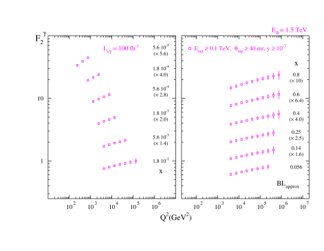
Figure 7.2: The kinematic coverage of the measurement of $F^{\gamma}_{2}$for the backscattered $e\gamma$ mode at a 3-TeV linear collider such as CLIC [23]

The $Q^{2}$ evolution of the structure function at large $x$ and $Q^{2}$ has often been advocated as a clean measurement of $\alpha_{s}$. It has been shown [23], however, that a 5% change on $\alpha_{s}$ results in a 3% change in $F^{\gamma}_{2}$only, hence such a $\alpha_{s}$ determination will require very precise $F^{\gamma}_{2}$measurements.

At very high values of $Q^{2}$ $\sim$ 10000 GeV², also $Z$ and $W$ exchange will become important, the latter leading to charged-current events [24] with large missing transverse momentum due to the escaping neutrino. By measuring the electroweak neutral and charged-current structure functions, the up- and down-type quark content of the photon can be determined separately.

A linear collider can also provide circularly-polarized photon beams, either from the polarized beams of the $e^{+}e^{-}$ collider directly, or via polarized laser beams scattered on the polarized $e^{+}e^{-}$ drive beam. This offers a unique opportunity to study the polarized parton distributions of the photon, for which no experimental data are available to date.

While $e\gamma$ scattering allows one to measure the quark distributions inside the photon, it constrains only weakly the gluon distribution via the QCD evolution of the structure functions. Direct information on the gluon in the photon can however be obtained from measurements of jet [25], open charm [26], and $J/\psi$ [27] production in $\gamma\gamma$ interactions at an $e^{+}e^{-}$ and $\gamma\gamma$ collider.

Dijet production in $\gamma\gamma$ interactions has been studied at CLIC energies. The two jets can be used to estimate the fraction of the photon momentum participating in the hard interaction, which is a sensitive probe of the structure of the photon. The transverse energy of the jets provides a hard scale, which allows such processes to be calculated in perturbative QCD. Fixed-order calculations at the next-to-leading order (NLO) in the strong coupling constant $\alpha_{\rm s}$ for dijet production are available and can be compared with the data, providing tests of the theory. Measurements of this kind are available from TRISTAN  [28, 29] and LEP [30, 31, 32]. The $k_{\perp}$-clustering algorithm [33] is used to define jets because of the advantages of this algorithm in the comparison to theoretical calculations [34]. The study is done using PHOJET [35] and PYTHIA [36] for an $e^{+}e^{-}$ centre-of-mass energy of 3 TeV with SIMDET modified for CLIC to simulate the detector response. HADES is used to provide additional $\gamma\gamma$ interactions.

For studies of the photon structure, a pair of variables, ${x_{\gamma}^{+}}$ and ${x_{\gamma}^{-}}$, is defined [37]. They estimate the fraction of the photon’s momentum participating in the hard scattering process:

$${x_{\gamma}^{+}}\equiv\frac{\displaystyle{\sum_{\rm jets=1,2}(E^{\mathrm{jet}}+p_{z}^{\mathrm{jet}})}}{{\displaystyle\sum_{\rm hfs}(E+p_{z})}}\qquad\mbox{and}\qquad{x_{\gamma}^{-}}\equiv\frac{\displaystyle{\sum_{\rm jets=1,2}(E^{\mathrm{jet}}-p_{z}^{\mathrm{jet}})}}{\displaystyle{\sum_{\rm hfs}(E-p_{z})}}\,,$$ (7.3)

where $p_{z}$ is the momentum component along the $z$ axis of the detector and $E$ is the energy of the jets or other hard objects in the hadronic final state (hfs). In leading order, for direct events, all the energy of the event is contained in two jets, i.e. ${{x_{\gamma}^{+}}}$ = 1 and ${{x_{\gamma}^{-}}}$ = 1, whereas for single-resolved or double-resolved events one or both values are smaller than 1. The dijet differential cross section as a function of ${x_{\gamma}}$ is therefore particularly well suited to study the structure of the photon, since it separates predominantly-direct events at high ${x_{\gamma}}$ (${x_{\gamma}}>$ 0.75) from predominantly-resolved events at low ${x_{\gamma}}$ (${x_{\gamma}}<$ 0.75). However, as is evident from the definition of ${x_{\gamma}}$, it is crucial to identify the two jets from the same $\gamma\gamma$ interaction if one is to gain access to the structure of the photon.

Figure 7.3 shows a generator study of the distribution of ${x_{\gamma}}$, for events in $e^{+}e^{-}$ collisions selected by having two jets with transverse energies above thresholds $E_{T}^{\rm jet1}>$ 10 GeV and $E_{T}^{jet2}>$ 8 GeV both in the region $|\eta|<$ 2.5, predicted for two different photon parametrizations. The measurements can go down to ${x_{\gamma}}\sim$ 5 $\times$ 10^-4. The difference between the two parton distributions gives a factor of 2 difference in the dijet cross sections in this kinematic region.

Figure 7.3: The ${x_{\gamma}}$ and ${\mathrm{log_{10}}(x_{\gamma})}$ cross sections for a single $\gamma\gamma$ collision, for different photon structure functions on a linear (top) and a logarithmic scale (bottom). The figures to the right show the ratio of the distributions of the two structure functions.

This measurement will have to be made at reduced luminosities. For the nominal high-luminosity scenario, it is expected that each bunch crossing will yield on average four $\gamma\gamma$ interactions. In addition, several bunch crossings may be overlaid; these, being genuine $\gamma\gamma$ interactions, are they part of the signal.

However, overlaid interactions would spoil the measurement, both by smearing the energy of the jets and by adding additional jets to the event, making it increasingly unlikely that the leading two jets originate from the same hard interaction. In addition, the extra energy added outside the two leading jets leads to a distortion of the ${x_{\gamma}}$ distribution towards lower values, as can be seen in Fig. 7.4.

Figure 7.4: The ${x_{\gamma}}$ and ${\mathrm{log_{10}}(x_{\gamma})}$ distributions for a single $\gamma\gamma$ collision compared with the case where one or two bunch crossings of $\gamma\gamma$ collisions are overlaid. The upper two plots require the first and second jets in the event to be above 7 GeV and 5 GeV transverse momentum. In the lower two plots the thresholds have been raised to 10 GeV and 8 GeV, respectively.

In addition to the type of physics studies mentioned above, the presence of many $\gamma\gamma$ collisions in each event has potentially severe implications for many other analyses. To investigate these effects, a dedicated study was carried out using PYTHIA for $Z$-pair production, where both $Z$ bosons decay exclusively to neutrinos. This process does not deposit any signal in the detector and enables us to study the effect of the hadronic background as simulated by HADES. This study demonstrates that even if the invariant mass of the hadronic system is required to be above 200 GeV, between 5 and 10 GeV per unit rapidity are added to the event, per bunch crossing. Furthermore, the visible transverse momentum of the hadronic final state rises as a function of the number of $\gamma\gamma$ collisions present. Figure 7.5 shows that, already for two bunch crossings, between 5 and 10 GeV of visible transverse momentum will be added to each event.

Figure 7.5: Visible transverse momentum of the hadronic final state contributed on average by background $\gamma\gamma$ collisions in one (solid), two (dashed) and eight (dotted) bunch crossings, as a function of the invariant mass of the hadronic final state. The vertical error bars indicate the spread.

7.4 Tests of BFKL Dynamics

One of the important open questions in high-energy QCD is the existence of BFKL effects. The BFKL equation [38, 39] resums multiple gluon radiation of the gluon exchanged in the $t$ channel, corresponding to a resummation of $\alpha_{s}\ln 1/x$ terms. It predicts a power increase of the cross section. HERA, the Tevatron and even LEP have been searching for BFKL effects in the data. Currently the situation is that in some corners of the phase space the NLO calculations undershoot the measured QCD activity, e.g. for forward jets and neutral pions at HERA, but the BFKL dynamics has not yet been established.

The BFKL dynamics can be tested at future high-energy $e^{+}e^{-}$ linear colliders. In this section, the total $\gamma^{*}\gamma^{*}$ cross section derived in the leading-logarithmic QCD dipole picture of BFKL dynamics is calculated, with higher-order corrections. The advantage of $\gamma^{*}\gamma^{*}$ scattering is that it is a process without non-perturbative couplings.

Defining $y_{1}$ ($y_{2}$) and $Q_{1}^{2}$ ($Q_{2}^{2}$) to be the rapidities and the squared transferred energies for the two virtual photons, one obtains [40, 41]

$$d\sigma_{e^{+}e^{-}}(Q_{1}^{2},Q_{2}^{2};y_{1},y_{2})=\frac{4}{9}\left(\frac{\alpha_{\rm em}^{2}}{16}\right)^{2}\,\alpha_{s}^{2}\,\pi^{2}\sqrt{\pi}\,\frac{dQ_{1}^{2}}{Q_{1}^{2}}\,\frac{dQ_{2}^{2}}{Q_{2}^{2}}\,\frac{dy_{1}}{y_{1}}\,\frac{dy_{2}}{y_{2}}\,\frac{1}{Q_{1}\,Q_{2}}\,$$

$$\frac{\exp\left(\frac{4\alpha_{s}N_{c}}{\pi}\,Y\ln 2\right)}{\sqrt{\frac{14\alpha_{s}N_{c}}{\pi}Y\zeta(3)}}\times\,\exp\left(-\frac{\ln^{2}\frac{Q_{1}^{2}}{Q_{2}^{2}}}{\frac{56\alpha_{s}N_{c}}{\pi}Y\zeta(3)}\right)\,\left[2l_{1}+9t_{1}\right]\,\left[2l_{2}+9t_{2}\right]\,,$$ (7.4)

for the leading-order BFKL cross section, where $t_{1}\equiv\frac{1}{2}(1+(1-y_{1})^{2}),\quad l_{1}\equiv 1-y_{1}$, $t_{2}$ and $l_{2}$ are defined analogously, and $Y\equiv\ln\left(sy_{1}y_{2}/\sqrt{Q^{2}_{1}Q^{2}_{2}}\right)$.

The two-gluon-exchange cross section has been calculated exactly in the high-energy approximation, and reads

$$d\sigma_{e^{+}e^{-}}(Q_{1}^{2},Q_{2}^{2};y_{1},y_{2}) = \frac{dQ_{1}^{2}}{Q_{1}^{2}}\,\frac{dQ_{2}^{2}}{Q_{2}^{2}}\,\frac{dy_{1}}{y_{1}}\,\frac{dy_{2}}{y_{2}}\,\frac{64\,(\alpha_{\rm em}^{2}\alpha_{s})^{2}}{243\pi^{3}}\,\frac{1}{Q_{1}^{2}}$$ (7.5)

$$\left[t_{1}t_{2}\ln^{3}\frac{Q_{1}^{2}}{Q_{2}^{2}}+\left(7t_{1}t_{2}+3t_{1}l_{2}+3t_{2}l_{1}\right)\ln^{2}\frac{Q_{1}^{2}}{Q_{2}^{2}}\right.$$

$$\left.+\left(\left(\frac{119}{2}-2\pi^{2}\right)t_{1}t_{2}+5(t_{1}l_{2}+t_{2}l_{1})+6l_{1}l_{2}\right)\ln\frac{Q_{1}^{2}}{Q_{2}^{2}}\right.$$

$$\left.+\left(\frac{1063}{9}-\frac{14}{3}\pi^{2}\right)t_{1}t_{2}+(46-2\pi^{2})(t_{1}l_{2}+t_{2}l_{1})-4l_{1}l_{2}\right]\,.$$

It is shown in Ref. [41] that the two-gluon cross section almost always dominates over the DGLAP one in the double-leading-logarithmic (DLL) approximation, and that the difference between the BFKL and two-gluon cross-sections increases with $Y$.

The comparison between the DGLAP-DLL and two-gluon cross sections in the leading-order (LO) approximation shows that they are similar when $Q_{1}$ and $Q_{2}$ are not too different, precisely in the kinematical domain where the BFKL cross section is expected to dominate. However, when $Q_{1}^{2}/Q_{2}^{2}$ is further away from 1, the LO two-gluon cross section is lower than the DGLAP one, especially at large $Y$. This suggests that the two-gluon cross section could be a good approximation to the DGLAP one if both were restricted to the region where $Q_{1}^{2}/Q_{2}^{2}$ is close to 1. In this section we use the exact two-gluon cross-section to evaluate the effect of the non-BFKL background, since the two-gluon term appears to constitute the dominant part of the DGLAP cross section in the region 0.5 $<Q_{1}^{2}/Q_{2}^{2}<$ 2.

The results given here are based on these calculations for a future Linear Collider (LC) with 500 GeV in the centre of mass, and either 3 or 5 TeV for CLIC. In general, $\gamma^{*}\gamma^{*}$ interactions are selected at $e^{+}e^{-}$ colliders by detecting in forward calorimeters scattered electrons that leave the beam pipe. For the LC, it has been argued [40] that angles as low as 20 mrad should be reached. Currently, angles down to 40 mrad are foreseen to be instrumented for a generic detector at CLIC.

Details of the calculation are discussed in Refs. [41, 42]. Higher-order (HO) effects are added to the LO BFKL calculation in a phenomenological way. The results of the BFKL and two-gluon cross sections are given in Table 7.2, assuming that tagging of scattered leptons can be done down to 40 mrad and to 50 (100) GeV at LC (CLIC). The ratio between HO BFKL and two-gluon cross sections is lower at CLIC than at LC, owing to the difference in phase space. We find that about 97 (28) events can be expected per year at CLIC operating at 3 (5) TeV.

Table 7.2: Final cross sections (in fb), for event selections described in the text

		BFKLHO	two-gluon	ratio
CLIC (3 TeV)		9.7E–2	3.7E–2	2.6
CLIC (5 TeV)		2.8E–2	1.1E–3	2.5
LC (500 GeV)		8.7	2.6	3.3

The HO BFKL and two-gluon cross sections for a 3 TeV CLIC are plotted in Fig. 7.6, as well as their ratio for different values of the tagging angle. As was already noted in Ref. [41], it is important to decrease the tagging angle to obtain a larger ratio and large values of the cross sections. The conclusions are similar for a 5 TeV machine.

Figure 7.6: The HO BFKL and two-gluon cross sections and their ratio as functions of the tagging angle for CLIC at 3 TeV. Leptons are tagged beyond 100 GeV.

Figure 7.7: The HO BFKL and two-gluon cross sections and their ratio as functions of the tagging energy for CLIC at 5 TeV. Leptons are tagged beyond 40 mrad.

The dependence on the tagging energy is studied in Fig. 7.7. The ratio between the HO BFKL and two-gluon cross sections remains almost constant, but lowering the tagging energy has an important effect on the cross-section value, and on the number of events expected per year. Another strategy to identify BFKL effects in the data is to study the energy or $Y$ dependence of the cross sections. To illustrate this, we show calculations of the HO BFKL and two-gluon cross sections, as well as their ratio, for given cuts on rapidity $Y$ in Table 7.3. We note that one could reach up to a factor 6 difference, while keeping a cross section measurable at CLIC, if one could tag leptons down to 25 mrad. If this is not possible, a cut on $Y$ at 8 would probably be sufficient to see BFKL effects.

Table 7.3: Final cross sections (in fb), for event selections described in the text, after different cuts on $Y$

$Y$ cut	BFKLNLO	Two-gluon	Ratio	BFKLNLO	Two-gluon	Ratio
	3 TeV	3 TeV	3 TeV	5 TeV	5 TeV	5 TeV
No cut	9.7E–2	3.7E–2	2.6	2.8E–2	1.1E–3	2.5
$Y\geq$ 8.	7.8E–3	1.6E–3	4.8	2.8E–3	6.2E–4	4.5
$Y\geq$ 9.	1.9E–3	3.1E–4	6.2	9.3E–4	1.6E–4	5.7
$Y\geq$ 9.	3.3E–2	4.4E–3	7.5	1.1E–2	1.8E–3	6.2
$\theta\geq$ 25 mrad

The $Y$ dependence of the cross section remains a powerful tool to increase this ratio, and is more sensitive to BFKL effects, even in the presence of large HO corrections. The uncertainty in the BFKL cross section after HO corrections is still quite large. Thus, measurements performed at a LC or CLIC should be compared with the precise calculation of the two-gluon cross section after the kinematical cuts described above, and any difference would be a sign of BFKL effects. A fit of these cross sections would then be made to determine the BFKL pomeron intercept after HO corrections as done, for instance, for LEP or HERA data [43].

Closely related to the $\gamma^{*}\gamma^{*}$measurement is vector-meson production, e.g. $\gamma\gamma$$\to J/\psi J/\psi$ or (at large $t$) $\gamma\gamma$$\to\rho\rho$, where the hard scale in the process is given by the $J/\psi$ mass or the momentum transfer $t$. The $J/\psi$ particles can be detected via their decays into leptons, and separated from the background through their peaks in the dilepton invariant mass spectra. Approximately 100 fully reconstructed 4-muon events are expected for 200 fb^-1 of luminosity for a 500 GeV $e^{+}e^{-}$ collider [44]. For this channel it is crucial that the decay muons and/or electrons can be measured to angles below 10 degrees in the experiment. Further processes, which are strongly sensitive to BFKL effects, include $e\gamma$ scattering with associated jet production [45], and $e^{+}e^{-}\to e^{+}e^{-}\gamma X$ and $\gamma\gamma\to\gamma X$ [46].

In summary, the study of these various processes will provide fundamental new insight into small-$x$ QCD physics, going beyond that obtainable from present accelerators and the LC.

Chapter 8 SUMMARY

The LHC will provide unique physics at the energy frontier in the TeV energy range, for many years after its commissioning. However, scenarios for physics in the TeV range generally have aspects that the LHC is unable to test. Electron–positron linear colliders can complement the LHC by producing directly new weakly-interacting particles and making possible precision studies. These are the core motivations for a linear collider with centre-of-mass energy in the TeV range. However, a complete understanding of physics in the TeV range may require a multi-TeV linear $e^{+}e^{-}$ collider, for which the only available candidate is CLIC.

Research and development work on the two-beam acceleration concept to be used in CLIC has been maturing over a number of years, with the CLIC Test Facilities 1 and 2 demonstrating many key aspects of the required technologies. There have, in particular, been significant advances in demonstrating the feasibility of the high frequency and high accelerating gradient central to the CLIC design, as well as the high geometrical stability that it would require. Based on these studies, parameter sets have been proposed for a nominal CLIC centre-of-mass energy of 3 TeV and for a possible upgrade to 5 TeV, as well as for lower-energy linear colliders based on CLIC technologies.

The high-energy CLIC parameter sets imply a large amount of beamstrahlung, which produces important photon and electron–positron pair-production backgrounds, as well as a relatively broad spectrum of beam collision energies. This study has shown that these are not insuperable barriers to experimentation at CLIC. There are designs for the beam-delivery system, interaction region and detector that reduce the beam-induced backgrounds sufficiently for all the essential physics measurements to be made. The concepts proposed for detectors at lower-energy linear colliders may be adapted for experiments at CLIC.

Likewise, studies for lower-energy colliders have developed tools for simulating physics events and backgrounds that serve also for experiments at CLIC. These tools include generators for Standard Model events and code suitable for modelling new physics processes. We note in particular that the electroweak radiative corrections to interesting physics processes are well understood, and can be calculated with sufficient accuracy to enable CLIC data to be interpreted reliably.

A key topic for experiments at CLIC will be the completion of the phenomenological profile of the Higgs boson. Within the Standard Model, CLIC will make it possible to determine whether a light candidate Higgs boson is indeed responsible for the muon mass. The higher centre-of-mass energy of CLIC will enable the triple-Higgs coupling of a light Higgs boson to be measured much more accurately than at lower-energy linear colliders. If there is a heavy SM Higgs boson, CLIC will enable it to be studied closely. If nature is described by supersymmetry, there will be more than one physical Higgs boson. CLIC will provide unparalleled reach for the heavier supersymmetric Higgs bosons, opening new possibilities for probing CP violation.

The relatively high centre-of-mass energy of CLIC will provide unique kinematic reach for the supersymmetric particles themselves. The luminosity offered by CLIC will be ample to study their masses and decays in detail. The strong beamstrahlung at CLIC will smear the centre-of-mass energy and complicate missing-energy analyses. However, studies of the production and decay of several species of supersymmetric particles, including smuons, selectrons, charginos and stop squarks demonstrate that these complications do not impede accurate measurements of sparticle masses and decays. In some supersymmetric scenarios, CLIC will produce many types of sparticle that are too heavy to be produced at a lower-energy linear collider. In other supersymmetric scenarios, CLIC will make possible precise measurements of strongly-interacting squarks and gluinos that cannot be performed at the LHC.

CLIC will likewise provide a unique kinematic reach for probing other theories of physics beyond the Standard Model, such as extra dimensions. In each of the cases studied, the experimental conditions at CLIC are no obstacle to exploiting fully the broad kinematic reach of CLIC.

There will also be unique opportunities at CLIC to study QCD. In addition to jet production and fragmentation studies in electron–positron annihilation events, CLIC will make possible detailed probes of QCD predictions in the collisions of real and virtual photons. In particular, the high CLIC centre-of-mass energy will enable BFKL predictions for high-energy scattering to be tested.

This exploratory study has demonstrated that experiments at CLIC will be able to exploit fully its high centre-of-mass energy for tests of the Standard Model as well as unique probes of ideas for new physics beyond the Standard Model. CLIC will take physics at the energy frontier to a new scale and level of accuracy.

References

- [1] The CLIC Study Team, ed. G. Guignard, ‘A 3 TeV linear collider based on CLIC technology’, CERN 2000-008 (2000).
- [2] H.H. Braun et al., ‘The CLIC RF power source – A novel scheme of two-beam acceleration for electron–positron linear colliders’, CERN 99-06 (1999).
- [3] S. Döbert, ‘Status of very high-gradient cavity tests’, in Proc. 21st International Linac Conference (LINAC 2002), Gyeongju, Korea, 19–23 Aug 2002, p. 276, CERN-CLIC-Note-533 (2002).
- [4] D. Schulte, ‘Luminosity limitations at the multi-TeV linear collider frontier’, in Proc. 8th European Particle Accelerator Conference, 3–7 June 2002, Paris, France, CLIC-Note 527.
- [5] H. Braun and D. Schulte, ‘Optimum coice of RF frequency for two beam linear colliders’, in Proc. Particle Accelerator Conference (PAC 03), Portland, Oregon, USA, 12–16 May 2003, CERN-CLIC-Note-563 (2003).
- [6] W. Wuensch et al., ‘A demonstration of high-gradient acceleration’, in Proc. Particle Accelerator Conference (PAC 03), Portland, Oregon, USA, 12–16 May 2003, CERN-CLIC-Note-569 (2003).
- [7] M. Korostelev and F. Zimmermann, ‘Optimization of CLIC damping ring design parameters’, in Proc. 8th European Particle Accelerator Conference, 3–7 June 2002, Paris, France.
- [8] T.E. D’Amico, G. Guignard and T. Raubenheimer, ‘The CLIC main linac bunch compressor’, in Proc. 6th European Particle Accelerator Conference (EPAC 98), Stockholm, Sweden, 22–26 Jun 1998, CERN-CLIC-Note-372 (1998).
- [9] T.E. D’Amico. Private communication.
- [10] D. Schulte, ‘Emittance preservation in the main linac of CLIC’, in Proc. 6th European Particle Accelerator Conference (EPAC 98), Stockholm, Sweden, 22–26 Jun 1998, CERN-CLIC-Note-320 (1998).
- [11] M. Aleksa et al., ‘Design status of the CLIC beam delivery system’, in Proc. 8th European Particle Accelerator Conference, 3–7 June 2002, Paris, France, CLIC-Note-521.
- [12] S. Redaelli et al., ‘The effect of cooling water on magnet vibration’, in Proc. 8th European Particle Accelerator Conference, 3–7 June 2002, Paris, France, CERN-CLIC-Note-531 (2002).
- [13] D. Schulte, ‘An update on the banana effect’, in Proc. 26th Advanced ICFA Beam Dynamics Workshop on Nanometer Size Colliding Beams, Lausanne, Switzerland, 2–6 Sep 2002, CLIC-Note-560 (2003).
- [14] D. Schulte, ‘Simulation of an intra-pulse interaction point feedback for future linear colliders’, in Proc. 20th International Linear Accelerator Conference, Monterey, CA, USA, 21–25 Aug 2000, CLIC-Note-454.
- [15] International Linear Collider Review Committee, Second Report 2003, SLAC-R-606.
- [16] J.-Y. Raguin, I. Wilson and W. Wuensch, ‘Progress in the design of a damped and tapered accelerating structure for CLIC’, in Proc. Particle Accelerator Conference (PAC 03), Portland, Oregon, USA, 12–16 May 2003, CERN-CLIC-Note-567 (2003).
- [17] ‘Zeroth order design report for the next linear collider’, SLAC-Report-474 (1996).
- [18] H. Tang et al., ‘The SLAC polarized electron source’, Talk at the 5th International Workshop on Polarized Beams and Polarized Gas Targets, Cologne, Germany, 6–9 Jun 1995, SLAC-PUB-6918 (1995).
- [19] T. Omori, ‘A polarized positron beam for linear coliders’, 1st ACFA Workshop on Physics Detector at the Linear Collider, Beijing, China, 26–28 Nov 1998, KEK-Preprint-98-237 (1999).
- [20] T. Omori, ‘A concept of a polarized positron source for a linear collider’, International Conference on Lasers’99, Quebec, Canada, Dec 13–17, 1999, KEK-Preprint-99-188 (2000).
- [21] T. Hirose et al., Nucl. Instrum. Meth. A455 (2000) 15.
- [22] R. Assmann and F. Zimmermann, CERN-SL-2001-064 AP, CERN-CLIC-NOTE-501 (2001).
- [23] V. Telnov, Nucl. Instrum. Meth. A472 (2001) 43, hep-ex/0010033.
- [24] B. Badelek et al., ‘TESLA technical design report’, Part VI, DESY 2001-011, hep-ex/0108012.
- [25] V. Telnov and H. Burkhardt, CERN-SL-2002-013 AP, CLIC-Note-508 (2002).
- [26] V. Telnov, Nucl. Instrum. Meth. A355 (1995) 3.
- [27] D. Schulte, Int. J. Mod. Phys. A18 (2003) 2851, CLIC-Note-512 (2002).
- [28] LC technology evaluation report 2001.
- [29] CERN/PS2002-008-RF, http://doc.cern.ch/archive/electronic/cern/preprints/ps/ps-2002-008.pdf .

References

- [1]
- [2] D. Schulte, ‘Beam–beam simulation with GUINEA-PIG’, ICAP98, Monterey, CA., USA, September 1998, CERN-PS-99-014 (LP).
-
[3]
D. Schulte and I. Syratchev,
‘Beam loading compensation in the main linac of CLIC’,
XX International Linac Conference, 21–25 August 2000, Monterey,
California, USA,
CERN-PS-2000-050-AE. -
[4]
M. Aleksa and S. Russenschuck,
‘Study of some options for the CLIC final focusing quadrupole’,
CLIC-Note-506 (2001). -
[5]
A. Drozhdin et al.,
‘Comparison of the TESLA, NLC and CLIC beam collimation systems
performance’,
Study Report of TRC Collimation Task Force (2002)
http://www-ap.fnal.gov/ drozhdin/prdriver/index.html . -
[6]
G.A Blair, ‘Simulation of the CLIC beam
delivery system using using BDSIM’,
CLIC-Note-509 (2002). - [7] G. Blair, H. Burkhardt and H.-J. Schreiber, ‘Background simulation for the CLIC beam delivery system with GEANT’, in Proc. 8th European Particle Accelerator Conference: a Europhysics Conference, La Villette, Paris, France, 3–7 Jun 2002, CERN-SL-2002-029.
- [8] M. Aleksa et al., ‘CLIC beam delivery system’, in Proc. 26th Advanced ICFA Beam Dynamics Workshop on Nanometer Size Colliding Beams (Nanobeam 2002), Lausanne, Switzerland, 2–6 Sep 2002, http://www.cern.ch/nanobeam .
- [9] F. Zimmermann et al., CERN-SL-2001-010-AP, CLIC-Note-476 (2001).
- [10] M. Aleksa et al., ‘Design status of the CLIC beam delivery system’, in Proc. 8th European Particle Accelerator Conference: a Europhysics Conference, La Villette, Paris, France, 3–7 Jun 2002, CERN-SL-2002-031 (2002).
- [11] R. Assmann et al., ‘Overview of the CLIC Collimation Design’, in Proc. IEEE Particle Accelerator Conference (PAC 2001), Chicago, Illinois, 18–22 Jun 2001, CLIC-Note-493, CERN-SL-2001-036-AP (2001).
- [12] M. Sachwitz and H.J. Schreiber (TESLA Collaboration), ‘Muon background in a 500-GeV TESLA linear collider’, TESLA-94-27.
- [13] M. Battaglia, Contributed talk to LCWS02, Jeju, Korea.
- [14] H. Burkhardt, S.R. Kelner and R.P. Kokoulin, ‘Monte Carlo generator for muon pair production’, CERN-SL-2002-016 (AP), CLIC-Note-511.
- [15] H. Burkhardt, S.R. Kelner and R.P. Kokoulin, ‘Production of muon pairs in annihilation of high-energy positrons with resting electrons’, CERN-AB-2003-002-ABP, CLIC-Note-554.
- [16] D. Schulte, ‘Study of electromagnetic and hadronic background in the interaction region of the TESLA collider’, PhD thesis, TESLA 97-08 (1996).
- [17] D. Schulte, ‘High energy beam–beam effects in CLIC’, in Proc. IEEE Particle Accelerator Conference (PAC 99), New York, 29 Mar – 2 Apr 1999, CERN-PS-99-017 (LP).
- [18] G.A. Schuler and T. Sjöstrand, CERN-TH/96-119 (1996).
- [19] HADES can be found at http://home.cern.ch/dschulte/physics/hades/hades.html .
- [20] D. Schulte, to be published.
- [21] D. Schulte, ‘Machine–detector interface at CLIC’, in Proc. 5th International Linear Collider Workshop (LCWS 2000), Fermilab, Batavia, Illinois, 24–28 Oct 2000, CERN-PS-2001-002-AE, CLIC-NOTE-469 (2001).
- [22] D. Schulte and F. Zimmermann, ‘The crossing angle in CLIC’, in Proc. IEEE Particle Accelerator Conference (PAC 2001), Chicago, Illinois, 18–22 Jun 2001, CERN-PS-2001-038-AE, CERN-SL-2001-043-AP.
- [23] S. Parker, C. Kenney and J. Segal, Nucl. Instrum. Meth. A395 (1997) 328.
- [24] C. Kenney, S. Parker and E. Walckiers, IEEE Trans. Nucl. Sci., 48 (2001) 2405.
- [25] TOTEM TDR, CERN-LHCC-2004-002, 7 January 2004, the publication on the test beam results reported in the TDR is in preparation.
- [26] C. Da Via’ et al., Nucl. Instrum. Meth. A509 (2003) 86.
- [27] G. Deputch, ‘New generation of monolithic active pixel sensors for charged particle detection’, PhD thesis, University of Strasbourg Louis Pasteur IReS, UMR7500, September 2002.
- [28] W. Dulinski et al., IEEE Nucl. Science Symposium Conf. Record (2001) IEEE 0-7803-7326-X.
- [29] N. Wyrsch et al., to appear in the Proc of the MRS Spring Meeting, San Francisco, CA, April 2003.
- [30] P. Jarron, A. Shah and N. Wyrsch, to appear in Proc. of the 9th Pisa Meeting on Advanced Detectors, Isola d’Elba, Italy, May 2003.
- [31] A. Albini et al., (NA1 Collaboration), Phys. Lett. B110 (1982) 339.
- [32] TESLA TDR/Part 4: Detector, T. Benhke et al., DESY-01-011D (2001).
- [33] J.C. Brient and H. Videau, ‘The calorimetry at the future linear collider’, in Proc. of APS/DPF/DPB Summer Study on the Future of Particle Physics (Snowmass 2001), Snowmass, Colorado, 30 Jun – 21 Jul 2001, eConf C010630 (2001) E3047, hep-ex/0202004.
- [34] R. Frey et al., SLAC-Pub 10171 (2002).
- [35] S. Jadach et al., Comput. Phys. Commun. 102 (1997) 229.
- [36] S. Jadach, W. Placzek and B.F. Ward, Phys. Lett. B353 (1995) 349.
- [37] D. Bardin, W. Hollik and G. Passarino (eds), Report of the Working Group on Precision Calculations for the Resonance, CERN-95-03.
- [38] A. Arbuzov et al., Phys. Lett. B383 (1996) 238, hep-ph/9605239.
- [39] B.F. Ward, S. Jadach, M. Melles and S.A. Yost, Phys. Lett. B450 (1999) 262, hep-ph/9811245.
- [40] D.Y. Bardin et al., Comput. Phys. Commun. 59 (1990) 303.
- [41] D.Y. Bardin et al., Comput. Phys. Commun. 133 (2001) 229, hep-ph/9908433.
- [42] H. Burkhardt and B. Pietrzyk, Phys. Lett. B356 (1995) 398.
- [43] S. Eidelman and F. Jegerlehner, Z. Phys. C67 (1995) 585.
- [44] H. Burkhardt and B. Pietrzyk, Phys. Lett. B513 (2001) 46.
- [45] F. Jegerlehner, ‘The effective fine structure constant at TESLA energies’, hep-ph/0105283.
- [46] K. Moenig, LC-PHSM-2000-060, Dec 2000.
- [47] P. Abreu et al., Note DELPHI 96-124 PHYS 632 (1996).
- [48] M. Peskin, Note LCC-0010 (1999).
- [49] S. Agostinelli et al., (GEANT4 Collaboration), ‘GEANT4 – A simulation toolkit’, SLAC-PUB-9350.
- [50] G.A. Blair, H. Burkhardt and H.J. Schreiber, ‘Background simulation for the CLIC beam delivery system with GEANT’, in Proc. 8th European Particle Accelerator Conference: a Europhysics Conference, La Villette, Paris, France, 3–7 Jun 2002, CERN-SL-2002-029.
- [51] D. Schulte et al., ‘CLIC simulations from the start of the linac to the interaction point, in Proc. of EPAC02.
- [52] G.A Blair, ‘Simulation of laser-wires at CLIC using BDSIM’, in Proc. of the Nanobeam Workshop, Lausanne, 2002.
- [53] A.A. Sokolov and I.M. Ternov, ‘Synchrotron radiation’, Pergamon Press, New York, (1968).
- [54] CALYPSO can be found at http://home.cern.ch/dschulte/physics/calypso/calypso.html .
-
[55]
HERWIG,
G. Corcella et al.,
JHEP 01 (2001) 010, hep-ph/0011363;
S. Moretti et al., JHEP 04 (2002) 028, hep-ph/0204123. -
[56]
ISAJET, H. Baer, F.E. Paige, S.D. Protopopescu and X. Tata,
hep-ph/0001086;
ISAJET is available from http://paige.home.cern.ch/paige/ . -
[57]
PYTHIA,
T. Sjostrand, L. Lonnblad and S. Mrenna, hep-ph/0108264;
T. Sjostrand et al., Comput. Phys. Commun. 135 (2001) 238, hep-ph/0010017;
PYTHIA is available from http://www.thep.lu.se/tf2/staff/torbjorn/Pythia.html . -
[58]
ARIADNE,
L. Lonnblad,
Comput. Phys. Commun. 71 (1992) 15;
ARIADNE is available from http://www.thep.lu.se/%7Eleif/ariadne/ . - [59] APACIC++, R. Kuhn et al., Comput. Phys. Commun. 134, 223 (2001), hep-ph/0004270.
-
[60]
M. Bertini, L. Lonnblad and T. Sjostrand,
Comput. Phys. Commun. 134 (2001) 365,
hep-ph/0006152. - [61] S. Gieseke, ‘Event generators: New developments’, hep-ph/0210294.
- [62] M. Kobel et al., ‘Two-fermion production in electron positron collisions’, hep-ph/0007180.
-
[63]
M.W. Grunewald et al.,
‘Four-fermion production in electron positron collisions’,
hep-ph/0005309. - [64] S. Jadach et al., (2000).
- [65] LUSIFER, S. Dittmaier and M. Roth, Nucl. Phys. B642 (2002) 307, hep-ph/0206070.
- [66] F. Caravaglios and M. Moretti, Phys. Lett. B358 (1995) 332, hep-ph/9507237.
- [67] G.P. Lepage, CLNS-80/447.
- [68] AMEGIC++, F. Krauss, R. Kuhn and G. Soff, JHEP 02 (2002) 044, hep-ph/0109036.
-
[69]
COMPHEP, A. Pukhov et al.,
‘CompHEP: A package for evaluation of Feynman diagrams and
integration over multi-particle phase space’,
hep-ph/9908288;
E. Boos et al. [CompHEP Collaboration], hep-ph/0403113;
COMPHEP is available from http://theory.sinp.msu.ru/comphep/ . -
[70]
GRACE, T. Ishikawa et al., (MINAMI-TATEYA group)
KEK-92-19;
GRACE is available from http://minami-home.kek.jp/ . - [71] G. Belanger et al., Phys. Lett. B559 (2003) 252 , hep-ph/0212261.
- [72] A. Kanaki and C.G. Papadopoulos, Comput. Phys. Commun. 132 (2000) 306, hep-ph/0002082.
- [73] C.G. Papadopoulos, Comput. Phys. Commun. 137 (2001) 247, hep-ph/0007335.
-
[74]
MADGRAPH/MADEVENT, F. Maltoni and T. Stelzer,
JHEP 02 (2003) 027, hep-ph/0208156;
T. Stelzer and W.F. Long, Comput. Phys. Commun. 81 (1994) 357, hep-ph/9401258;
MADGRAPH/MADEVENT is available from http://madgraph.physics.uiuc.edu/ . -
[75]
M. Moretti, T. Ohl and J. Reuter,
‘O’Mega: An optimizing matrix element generator’,
hep-ph/0102195. -
[76]
J. Kublbeck, M. Bohm and A. Denner,
Comput. Phys. Commun. 60 (1990) 165;
T. Hahn and M. Perez-Victoria, Comput. Phys. Commun. 118 (1999) 153;
T. Hahn, Comput. Phys. Commun. 140 (2001) 418;
FeynArts is available from http://www.feynarts.de/ . - [77] A. Denner et al., Nucl. Phys. B660 (2003) 289.
-
[78]
A. Djouadi, J.L. Kneur and G. Moultaka,
‘SuSpect: A Fortran code for the supersymmetric and Higgs
particle spectrum in the MSSM’,
hep-ph/0211331;
SuSpect is available from http://www.lpm.univ-montp2.fr:6714/kneur/Suspect/ . - [79] A. Djouadi et al., (MSSM Working Group Collaboration) ‘The minimal supersymmetric standard model: Group summary report’, hep-ph/9901246.
-
[80]
B.C. Allanach,
Comput. Phys. Commun. 143 (2002) 305, hep-ph/0104145;
SOFTSUSY is available from http://allanach.home.cern.ch/allanach/softsusy.html . -
[81]
W. Porod,
Comput. Phys. Commun. 153 (2003) 275, hep-ph/0301101;
SPHENO is available from http://www-theorie.physik.unizh.ch/porod/SPheno.html . -
[82]
M. Carena, J. Espinosa, M. Quiros and C. Wagner,
Phys. Lett. B335 (1995) 209;
Subhpole is available from http://fnth37.fnal.gov/higgs/carenawagner.html . - [83] H. Haber, R. Hempfling and A. Hoang, Z. Phys. C75 (1997) 539.
-
[84]
S. Heinemeyer, W. Hollik and G. Weiglein,
‘FeynHiggsFast: A program for a fast calculation of masses and
mixing angles in the Higgs sector of the MSSM’,
hep-ph/0002213;
FeynHiggsFast is available from http://www.feynhiggs.de/ . -
[85]
S. Heinemeyer, W. Hollik and G. Weiglein,
Comput. Phys. Commun.
124 (2000) 76;
FeynHiggs is available from http://www.feynhiggs.de/ . -
[86]
G. Degrassi, P. Slavich and F. Zwirner,
Nucl. Phys. B611 (2001) 403;
A. Brignole et al., Nucl. Phys. B631 (2002) 195, B643 (2002) 79. - [87] D.M. Pierce, J.A. Bagger, K. Matchev and R.J. Zhang, Nucl. Phys. B491 (1997) 3.
-
[88]
B. Allanach, S. Kraml and W. Porod,
‘Comparison of SUSY mass spectrum calculations’,
hep-ph/0207314. -
[89]
N. Ghodbane,
‘SUSYGEN3: An event generator for linear colliders’,
hep-ph/9909499;
S. Katsanevas and P. Morawitz, Comput. Phys. Commun. 112 (1998) 227, hep-ph/9711417;
SUSYGEN is available from http://lyoinfo.in2p3.fr/susygen/susygen3.html . -
[90]
P. Janot, in the report ‘Physics at LEP2’,
CERN-96-01-V-1;
HZHA is available from http://alephwww.cern.ch/janot/Generators.html . - [91] A. Djouadi, available at: http://djouadi.home.cern.ch/djouadi/ .
-
[92]
HDECAY,
A. Djouadi, J. Kalinowski and M. Spira,
Comput. Phys. Commun. 108 (1998) 56;
HDECAY is available from http://mspira.home.cern.ch/mspira/hdecay/ . - [93] A. Djouadi, Y. Mambrini and M. Mühlleitner, to appear.
- [94] P. Richardson, JHEP 11 (2001) 029, hep-ph/0110108.
- [95] J. Fleischer, A. Leike, T. Riemann and A. Werthenbach, ‘Electroweak one-loop corrections for annihilation into including hard bremsstrahlung’, DESY 02-204, CERN-TH-2003-023 (2003), hep-ph/0302259.
- [96] M. Kuroda, G. Moultaka and D. Schildknecht, Nucl. Phys. B350 (1991) 25.
- [97] W. Beenakker et al., Nucl. Phys. B410 (1993) 245; Phys. Lett. B317 (1993) 622.
- [98] P. Ciafaloni and D. Comelli, Phys. Lett. B446 (1999) 278.
-
[99]
M. Beccaria et al., Phys. Rev. D61 (2000) 073005;
M. Beccaria, F.M. Renard and C. Verzegnassi, Phys. Rev. D63 (2001) 053013; Phys. Rev. D64 (2001) 073008. - [100] J. Layssac and F.M. Renard, Phys. Rev. D64 (2001) 053018.
- [101] A. Denner and S. Pozzorini, Eur. Phys. J. C18 (2001) 461; Eur. Phys. J. C21 (2001) 63.
-
[102]
V.V. Sudakov, Sov. Phys. JETP 3 (1956) 65;
V.G. Gorshkov et a.l, Phys. Lett. 22 (1966) 671. - [103] J.H. Kühn, S. Moch, A.A. Penin and V.A. Smirnov, Nucl. Phys. B616 (2001) 286.
- [104] P. Ciafaloni and D. Comelli, Phys. Lett. B476 (2000) 49.
-
[105]
V.S. Fadin et al., Phys. Rev. D61 (2000) 094002;
M. Melles, Phys. Rep. 375 (2003) 219. - [106] J.H. Kühn, A.A. Penin and V.A. Smirnov, Eur. Phys. J. C17 (2000) 97.
-
[107]
M. Ciafaloni, P. Ciafaloni and D. Comelli, Nucl. Phys. B589 (2000) 359;
Phys. Lett. B501 (2001) 216. - [108] F. Bloch and A. Nordsieck, Phys. Rev. 52 (1937) 54.
- [109] W. Beenakker and A. Werthenbach, Phys. Lett. B489 (2000) 148.
- [110] M. Hori, H. Kawamura and J. Kodaira, Phys. Lett. B491 (2000) 275.
- [111] M. Melles, Phys. Lett. B495 (2000) 81.
- [112] W. Beenakker and A. Werthenbach, Nucl. Phys. B630 (2002) 3.
-
[113]
R.G. Stuart, Phys. Lett. B262 (1991) 113;
A. Aeppli, G.J. van Oldenborgh and D. Wyler, Nucl. Phys. B428 (1994) 126;
W. Beenakker and A. Denner, Int. J. Mod. Phys. A9 (1994) 4837. - [114] M. Ciafaloni, P. Ciafaloni and D. Comelli, Phys. Rev. Lett. 88 (2002) 102001.
- [115] A. Denner, M. Melles and S. Pozzorini, Nucl. Phys. B662 (2003) 299, hep-ph/0301241.
- [116] M. Melles, Eur. Phys. J. C24 (2002) 193.
- [117] E. Accomando et al., Phys. Rep. 299 (1998) 1;
- [118] J.A. Aguilar-Saavedra et. al. (ECFA/DESY LC Physics Working Group Collaboration), ‘TESLA Technical Design Report Part III: Physics at an Linear Collider’, hep-ph/0106315.
-
[119]
T. Abe et al. (American Linear Collider Working Group Collaboration),
‘Linear collider physics resource book for Snowmass 2001. 2: Higgs and
supersymmetry studies’,
in Proc. of the APS/DPF/DPB Summer Study on the Future of Particle
Physics (Snowmass 2001), ed. N. Graf,
hep-ex/0106056. -
[120]
J. Fleischer, T. Hahn, W. Hollik, T. Riemann, C. Schappacher and
A. Werthenbach,
‘Complete electroweak one-loop radiative corrections to top-pair
production at TESLA: A comparison’,
LC-TH-2002-002, hep-ph/0202109. - [121] M. Tentyukov and J. Fleischer, Comput. Phys. Commun. 132 (2000) 124.
-
[122]
M. Tentyukov and J. Fleischer,
‘DIANA, a program for Feynman diagram evaluation’,
hep-ph/9905560. - [123] J. Fleischer and F. Jegerlehner, Phys. Rev. D23 (1981) 2001.
- [124] D. Bardin and N. Shumeiko, Nucl. Phys. B127 (1977) 242.
- [125] G. Passarino, Nucl. Phys. B204 (1983) 237.
- [126] J. Fleischer, A. Leike and T. Riemann and A. Werthenbach, Fortran program topfit.F v.0.91
- [127] J. Fleischer et al., ‘One-loop corrections to the process including hard bremsstrahlung’, hep-ph/0203220.
- [128] J. Fleischer, A. Leike, T. Riemann and A. Werthenbach, ‘Status of electroweak corrections to top pair production’, DESY-02-203 (2002), hep-ph/0211428.
-
[129]
T. Hahn and M. Perez-Victoria,
Comput. Phys. Commun. 118 (1999) 153;
http://www.feyn-arts.de/looptools .

References

-
[1]
P.W. Higgs, Phys. Rev. Lett. 12 (1964) 132,
Phys. Rev. 145 (1966) 1156;
F. Englert and R. Brout, Phys. Rev. Lett. 13 (1964) 321;
G.S. Guralnik, C.R. Hagen and T.W. Kibble, Phys. Rev. Lett. 13 (1964) 585. - [2] R. Barate et al., Phys. Lett. B565 (2003) 61, hep-ex/0306033 .
- [3] M.W. Grünewald, Nucl. Phys. Proc. Suppl. 117 (2003) 280, hep-ex/0210003.
- [4] J.D. Hobbs, ‘Standard Model Higgs Prospects at the Tevatron’, in Proc. APS/DPF/DPB Summer Study on the Future of Particle Physics (Snowmass 2001), ed. N. Graf, Snowmass, Colorado, 30 Jun – 21 Jul 2001, eConf C010630 (2001) P103.
-
[5]
S. Abdullin et al., CMS-Note-2003/033;
D. Cavalli et al., ‘The Higgs Working Droup: Summary report’, in Proc. Workshop on Physics at TeV Colliders, Les Houches, France, 21 May – 1 Jun 2001, hep-ph/0203056. - [6] K. Desch, ‘Higgs Boson Precision Studies at a Linear Collider’, in Proc. 4th ECFA/DESY Workshop on Physics and Detectors for a 90-GeV to 800-GeV Linear Collider, Amsterdam, The Netherlands, 1–4 Apr 2003, hep-ph/0311092.
- [7] The Muon Collider Collaboration, http://www.cap.bnl.gov/mumu/ .
- [8] The VLHC, Snowmass report 2001.
- [9] F. Boudjema and E. Chopin, Z. Phys. C73 (1996) 85.
- [10] V. Barger, T. Han, P. Langacker, B. McElrath and P.M. Zerwas, Phys. Rev. D67 (2003) 115001.
-
[11]
A. Djouadi, W. Kilian, M. Muhlleitner and P.M. Zerwas,
Eur. Phys. J. C10 (1999) 27,
hep-ph/9903229. - [12] C. Castanier, P. Gay, P. Lutz and J. Orloff, ‘Higgs self coupling measurement in collisions at center-of-mass energy of 500-GeV’, in ‘2nd ECFA/DESY Study 1998–2001’ pp. 1362-1372, hep-ex/0101028.
-
[13]
M. Battaglia, E. Boos and W. M. Yao,
‘Studying the Higgs potential at the linear collider’,
in Proc. of the APS/DPF/DPB Summer Study on the Future of Particle
Physics (Snowmass 2001), ed. N. Graf, Snowmass, Colorado, 30 Jun –
21 Jul 2001,
eConf C010630 (2001) E3016,
hep-ph/0111276. - [14] LEP Electrowaek workking group, ‘A Combination of Preliminary Electroweak Measurements and Constrains on the Standard Model’, hep-ex/0312023.
- [15] M. Battaglia, ‘Physics Signatures at CLIC’, in ‘2nd ECFA/DESY Study 1998–2001’ pp. 2475-2489, CERN-CLIC-Note-474 (2001), hep-ph/0103338.
- [16] M. Battaglia et al., Eur. Phys. J. C22 (2001) 535.
- [17] M. Battaglia, A. Ferrari and A. Kiiskinen, in Proc. of the APS/DPF/DPB Summer Study on the Future of Particle Physics (Snowmass 2001), ed. N. Graf, Snowmass, Colorado, 30 Jun – 21 Jul 2001, eConf C010630 (2001) E3066, hep-ph/0111307.
-
[18]
I.F. Ginzburg, G.L. Kotkin, V.G. Serbo and V.I. Telnov,
JETP Lett. 34 (1981) 491
[Pisma Zh. Eksp. Teor. Fiz. 34 (1981) 514],
Nucl. Instrum. Meth. 205 (1983) 47;
I.F. Ginzburg et al., Nucl. Instrum. Meth. A219 (1984) 5. -
[19]
M.M. Mühlleitner, PhD thesis, DESY-THESIS-2000-033,
hep-ph/0008127;
M.M. Mühlleitner, M. Krämer, M. Spira and P.M. Zerwas, Phys. Lett. B508 (2001) 311. - [20] A. Djouadi, M. Spira and P.M. Zerwas, Z. Phys. C70 (1996) 427.
- [21] A. Djouadi, J. Kalinowski and M. Spira, Comput. Phys. Comm. 108 (1998) 56.
-
[22]
A. Djouadi et al., Phys. Lett. B257 (1991) 187,
Phys. Lett. B311 (1993) 255;
K. Melnikov and O. Yakovlev, Phys. Lett. B312 (1993) 179;
M. Inoue et al., Mod. Phys. Lett. A9 (1994) 1189;
M. Spira et al., Nucl. Phys. B453 (1995) 17;
E. Braaten and J.P. Leveille, Phys. Rev. D22 (1980) 715;
N. Sakai, Phys. Rev. D22 (1980) 2220;
T. Inami and T. Kubota, Nucl. Phys. B179 (1981) 171;
S.G. Gorishny et al., Sov. J. Nucl. Phys 40 (1984) 329;
M. Drees and K. Hikasa, Phys. Rev. D41 (1990) 1547, Phys. Lett. B240 (1990) 455,
(Erratum) B262 (1991) 497. -
[23]
B. Kamal et al., Phys. Rev. D51 (1995) 4808, (Erratum)
D55 (1997) 3229;
G. Jikia and A. Tkabladze, Phys. Rev. D54 (1996) 2030, Phys. Rev. D63 (2001) 074502. - [24] J.H. Kühn, E. Mirkes and J. Steegborn, Z. Phys. C57 (1993) 615.
- [25] H.J. Schreiber (TESLA Collaboration), private communication.
-
[26]
V.S. Fadin et al., Phys. Rev. D56 (1997) 484;
M. Melles and W.J. Stirling, Phys. Rev. D59 (1999) 094009, Eur. Phys. J. C9 (1999) 101, Nucl. Phys. B564 (2000) 325. - [27] S.Y. Choi, J. Kalinowski, J.S. Lee, M.M. Mühlleitner, M. Spira and P.M. Zerwas, hep-ph/0404119.
- [28] M. Carena, J.R. Ellis, S. Mrenna, A. Pilaftsis and C.E.M. Wagner, Nucl. Phys. B659 (2003) 145, hep-ph/0211467.
-
[29]
For recent analyses of one- and two-loop EDM effects, see
T. Ibrahim and P. Nath, Phys. Rev. D58 (1998) 111301, hep-ph/9807501; Phys. Rev. D61 (2000) 093004, hep-ph/9910553;
M. Brhlik, G.J. Good and G.L. Kane, Phys. Rev. D59 (1999) 115004, hep-ph/9810457;
S. Pokorski, J. Rosiek and C.A. Savoy, Nucl. Phys. B570 (2000) 81, hep-ph/9906206;
E. Accomando, R. Arnowitt and B. Dutta, Phys. Rev. D61 (2000) 115003, hep-ph/9909333;
A. Bartl, T. Gajdosik, W. Porod, P. Stockinger and H. Stremnitzer, Phys. Rev. D60 (1999) 073003, hep-ph/9903402;
D. Chang, W.-Y. Keung and A. Pilaftsis, Phys. Rev. Lett. 82 (1999) 900, hep-ph/9811202;
S.A. Abel, S. Khalil and O. Lebedev, Nucl. Phys. B606 (2001) 151, hep-ph/0103320;
D.A. Demir, M. Pospelov and A. Ritz, Phys. Rev. D67 (2003) 015007, hep-ph/0208257. -
[30]
For a recent analysis of Higgs-mediated EDMs in the
CP-violating MSSM, see
A. Pilaftsis, Nucl. Phys. B644 (2002) 263, hep-ph/0207277. - [31] T. Falk, K.A. Olive, M. Pospelov and R. Roiban, Nucl. Phys. B60 (1999) 3, hep-ph/9904393.
-
[32]
For example, see,
A.J. Buras, P.H. Chankowski, J. Rosiek and L. Slawianowska, Nucl. Phys. B619 (2001) 434,
hep-ph/0107048; Nucl. Phys. B659 (2003) 3, hep-ph/0210145;
P.H. Chankowski and L. Slawianowska, Acta Phys. Polon. B32 (2001) 1895;
C.S. Huang and W. Liao, Phys. Lett. B538 (2002) 301, hep-ph/0201121;
D.A. Demir and K.A. Olive, Phys. Rev. D65 (2002) 034007 hep-ph/0107329;
T. Ibrahim and P. Nath, Phys. Rev. D67 (2003) 016005, hep-ph/0208142. - [33] A. Dedes and A. Pilaftsis, Phys. Rev. D67 (2003) 015012, hep-ph/0209306.
-
[34]
A. Pilaftsis,
Phys. Rev. D58 (1998) 096010,
hep-ph/9803297;
Phys. Lett. B435 (1998) 88,
hep-ph/9805373. - [35] A. Pilaftsis and C.E.M. Wagner, Nucl. Phys. B553 (1999) 3, hep-ph/9902371.
-
[36]
D. Demir, Phys. Rev. D60 (1999) 055006, hep-ph/9901389;
S. Choi, M. Drees and J. Lee, Phys. Lett. B481 (2000) 57, hep-ph/0002287. -
[37]
S. Heinemeyer, Eur. Phys. Jour. C22 (2001) 521,
hep-ph/0108059;
M. Frank, S. Heinemeyer, W. Hollik and G. Weiglein, in preparation. - [38] M. Carena, J. Ellis, A. Pilaftsis and C.E.M. Wagner, Nucl. Phys. B586 (2000) 92, hep-ph/0003180.
-
[39]
T. Banks, Nucl. Phys. B303 (1988) 172;
L. Hall, R. Rattazzi and U. Sarid, Phys. Rev. D50 (1994) 7048, hep-ph/9306309;
R. Hempfling, Phys. Rev. D49 (1994) 6168;
M. Carena, M. Olechowski, S. Pokorski and C. Wagner, Nucl. Phys. B426 (1994) 269,
hep-ph/9402253. -
[40]
A. Méndez and A. Pomarol,
Phys. Lett. B272 (1991) 313;
J.F. Gunion, B. Grzadkowski, H.E. Haber and J. Kalinowski, Phys. Rev. Lett. 79 (1997) 982,
hep-ph/9704410. - [41] M. Carena, J. Ellis, A. Pilaftsis and C. Wagner, Phys. Lett. B495 (2000) 155, hep-ph/0009212.
- [42] M. Frank, PhD thesis, university of Karlsruhe, 2002.
-
[43]
K. Desch, Z. Was and M. Worek,
Eur. Phys. J. C29 (2003) 491,
hep-ph/0302046;
K. Desch, private communication. -
[44]
S. Heinemeyer, W. Hollik and G. Weiglein,
Comp. Phys. Comm. 124 2000 76,
hep-ph/9812320;
The codes are accessible via www.feynhiggs.de . -
[45]
M. Frank, S. Heinemeyer, W. Hollik and G. Weiglein,
hep-ph/0212037;
T. Hahn, S. Heinemeyer, W. Hollik and G. Weiglein, in preparation. -
[46]
S. Heinemeyer, W. Hollik, J. Rosiek, and G. Weiglein,
Eur. Phys. J. C19 (2001) 535,
hep-ph/0102081. - [47] E. Christova, H. Eberl, W. Majerotto and S. Kraml, Nucl. Phys. B639 (2002) 263, hep-ph/0205227.

References

-
[1]
See for instance,
H.P. Nilles, Phys. Rep. 110 (1984) 1;
H.E. Haber and G.L. Kane, Phys. Rep. 117 (1985) 75. -
[2]
L. Maiani, in Proc. of the 1979 Gif-sur-Yvette Summer School on
Particle Physics, 1;
G. ’t Hooft, Recent Developments in Gauge Theories, in Proc. of Advanced Study Institute, Cargēse, 1979, eds. G. ’t Hooft et al., Plenum Press, NY, 1980;
E. Witten, Phys. Lett. B105, 267 (1981). -
[3]
H. Haber and R. Hempfling,
Phys. Rev. Lett. 66 (1991) 1815;
M. Carena, M. Quirós and C.E.M. Wagner, Nucl. Phys. B461 (1996) 407;
H. Haber, R. Hempfling and A. Hoang, Z. Phys. C75 (1997) 539;
S. Heinemeyer, W. Hollik and G. Weiglein, Phys. Rev. D58 (1998) 091701, Eur. Phys. J. C9 (1999) 343;
R.-J. Zhang, Phys. Lett. B447 (1999) 89. - [4] LEP Higgs Working Group for Higgs Boson Searches Collaboration, ‘Search for the Standard Model Higgs boson at LEP’, contributed to International Europhysics Conference on High Energy Physics (HEP 2001), Budapest, Hungary, 12–18 Jul 2001, hep-ex/0107029.
- [5] J. Erler, Phys. Rev. D63 (2001) 071301, hep-ph/0010153.
-
[6]
J. Ellis, S. Kelley and D.V. Nanopoulos,
Phys. Lett. B260 (1991)131;
U. Amaldi, W. de Boer and H. Furstenau, Phys. Lett. B260 (1991) 447;
P. Langacker and M. Luo, Phys. Rev. D44 (1991) 817;
C. Giunti, C.W. Kim and U.W. Lee, Mod. Phys. Lett. A6 (1991) 1745. -
[7]
J.R. Ellis et al.,
Nucl. Phys. B238 (1984) 453;
see also H. Goldberg, Phys. ReV. Lett. 50 (1983) 1419. - [8] M. Battaglia et al., Eur. Phys. J. C33 (2004) 273, hep-ph/0306219.
- [9] M. Battaglia et al., Eur. Phys. J. C22 (2001) 535.
-
[10]
C.L. Bennett et al.,
Astrophys. J. Suppl. 148 (2003) 1, astro-ph/0302207;
H.V. Peiris et al., Astrophys. J. Suppl. 148 (2003) 213, astro-ph/0302225. - [11] ATLAS Collaboration, ‘ATLAS: Detector and Physics Performance Technical Design Report’, CERN-LHCC 99-14/15 (1999).
-
[12]
S. Abdullin et al., (CMS Collaboration),
J. Phys. G28 (2002) 469, hep-ph/9806366;
S. Abdullin and F. Charles, Nucl. Phys. B547 (1999) 60;
CMS Collaboration, Technical Proposal, CERN-LHCC 94-38 (1994). - [13] G. Blair, W. Porod and P.M. Zerwas, Phys. Rev. D63 (2001) 017703, hep-ph/0007107.
- [14] B.C. Allanach et al., Eur. Phys. J. C25 (2002) 113.
- [15] G.L. Kane et al., Phys. Rev. D67 (2003) 045008.
- [16] J. Feng and D. Finnell, Phys. Rev. D49 (1994) 2369.
- [17] D. Denegri, W. Majerotto and L. Rurua, Phys. Rev. D58 (1998) 095010, hep-ph/9711357.
- [18] H.U. Martyn, contributed to Workshop on Physics at TeV Colliders, Les Houches, France, 7–18 Jun 1999, hep-ph/0002290.
- [19] G.A. Blair, ‘Sparticle masses and widths via threshold scans at the linear collider’, in Proc. of the APS/DPF/DPB Summer Study on the Future of Particle Physics (Snowmass 2001), ed. N. Graf, Snowmass, Colorado, 30 Jun – 21 Jul 2001, eConf C010630 (2001) E3019.
- [20] M. Drees and K. Hikasa, Phys. Lett. B252 (1990) 127.
- [21] S. Kraml, ‘Stop and sbottom phenomenology in the MSSM’, Ph.D. Thesis, hep-ph/9903257.
- [22] S. Heinemeyer, S. Kraml, W. Porod and G. Weiglein, JHEP 0309 (2003) 075, hep-ph/0306181.
-
[23]
G. Belanger, F. Boudjema, T. Kon and V. Lafage,
Eur. Phys. J. C9 (1999) 511, hep-ph/9811334;
A. Djouadi, J.L. Kneur and G. Moultaka, Nucl. Phys. B569 (2000) 53, hep-ph/9903218. - [24] A. Bartl et al., Phys. Lett. B435 (1998) 118, hep-ph/9804265.
- [25] S. Berge and M. Klasen, Phys. Rev. D66 (2002) 115014.
- [26] S. Berge and M. Klasen, Eur. Phys. J. C30 (2003) 123, hep-ph/0303032.
- [27] H. Burkhardt and V. Telnov, ‘CLIC 3-TeV photon collider option’, CERN-SL-2002-013-AP.
- [28] T. Affolder et al. (CDF Collaboration), Phys. Rev. Lett. 88 (2002) 041801.
- [29] S. Abachi et al. (D0 Collaboration), Phys. Rev. Lett. 75 (1995) 618.
- [30] LEP Higgs Working Group Collaboration, Note 2001-04, ‘Searches for the neutral Higgs bosons of the MSSM: Preliminary combined results using LEP data collected at energies up to 209 GeV’, hep-ex/0107030.
- [31] T. Hahn and C. Schappacher, Comput. Phys. Commun. 143 (2002) 54, hep-ph/0105349.
- [32] K. Hagiwara et al. (Particle Data Group Collaboration), Phys. Rev. D66 (2002) 010001.
- [33] J. Abdallah et al. (LEP SUSY Working Group Collaboration), http://lepsusy.web, cern.ch/lepsusy .
- [34] T. Hahn, Comput. Phys. Commun. 140 (2001) 418, hep-ph/0012260.
- [35] T. Hahn and M. Perez-Victoria, Comput. Phys. Commun. 118 (1999) 153, hep-ph/9807565.
- [36] A. Airapetian et al. (ATLAS Collaboration), ‘ATLAS Detector and Physics Performance. Technical design report’, Vol. 2, CERN-LHCC-99-15.
- [37] S. Abdullin et al. (CMS Collaboration), J. Phys. G28 (2002) 469, hep-ph/9806366.
- [38] M. Battaglia et al., Eur. Phys. J. C22 (2001) 535, hep-ph/0106204.
- [39] G. Blair, W. Porod and P.M. Zerwas, Eur. Phys. J. C27 (2003) 263, hep-ph/0210058.
- [40] W. Porod, Comput. Phys. Commun. 153 (2003) 275, hep-ph/0301101.
-
[41]
J. Aguilar-Saavedra et al.,
‘Physics at an Linear Collider’,
TESLA TDR Part 3,
hep-ph/0106315. - [42] F. James and M. Roos, Comput. Phys. Commun. 10 (1975) 343.
- [43] D. Pierce et al., Nucl. Phys. B491 (1997) 3, hep-ph/9606211.
-
[44]
G. Degrassi, P. Slavich and F. Zwirner,
Nucl. Phys. 611 (2001) 403,
hep-ph/0105096;
A. Brignole et al., Nucl. Phys. B631 (2002) 195, hep-ph/0112177;
A. Dedes and P. Slavich, Nucl. Phys. B657 (2003) 333, hep-ph/0212132. - [45] M. Drees and K. Hikasa, Phys. Lett. B252 (1990) 127.
- [46] H. Eberl, A. Bartl and W. Majerotto, Nucl. Phys. B472 (1996) 481, hep-ph/9603206.
- [47] A. de Roeck, private communication.
- [48] E. Boos et al., Eur. Phys. J. C30 (2003) 395, hep-ph/0303110.
- [49] A. Bartl, K. Hidaka, T. Kernreiter and W. Porod, Phys. Rev. D66 (2002) 115009, hep-ph/0207186.
-
[50]
G. Moortgat-Pick and H.M. Steiner,
Eur. Phys. J. direct C3 (2001) 6, hep-ph/0106155;
see also, G. Moortgat-Pick, hep-ph/0303234, hep-ph/0106315. -
[51]
J. Fleischer, K. Kolodziej and F. Jegerlehner,
Phys. Rev. D49 (1994) 2174;
see also K. Desch, talk at International Workshop on Linear Colliders, August 26–30, 2002, Jeju Island, Korea: http://lcws2002.korea.ac.kr/ . - [52] P. Chiappetta et al., Nucl. Phys. B259 (1985) 365.
- [53] C. Blochinger et al., Eur. Phys. J. C24 (2002) 297, hep-ph/0201282.
-
[54]
B. C. Allanach et al.,
Eur. Phys. J. C25 (2002) 113
[eConf C010630 (2001) P125], hep-ph/0202233;
N. Ghodbane and H.U. Martyn, ‘Compilation of SUSY particle spectra from Snowmass 2001 benchmark models’, in Proc. of the APS/DPF/DPB Summer Study on the Future of Particle Physics (Snowmass 2001), ed. N. Graf, Snowmass, Colorado, 30 Jun – 21 Jul 2001, hep-ph/0201233. -
[55]
S.Y. Choi, J. Kalinowski, G. Moortgat-Pick and P.M. Zerwas,
Eur. Phys. J. C22 (2001) 563,
hep-ph/0108117; C23 (2002) 769, hep-ph/0202039. -
[56]
A. Freitas et al.,
hep-ph/0211108;
A. Freitas and A. von Manteuffel, hep-ph/0211105. -
[57]
S. Hesselbach, F. Franke and H. Fraas,
hep-ph/0003272;
F. Franke and S. Hesselbach, Phys. Lett. B526 (2002) 370, hep-ph/0111285;
G. Moortgat-Pick, S. Hesselbach, F. Franke and H. Fraas, hep-ph/9909549. -
[58]
H. Baer et al.,
Phys. Rev. D59 (1999) 055014, hep-ph/9809223;
V.D. Barger, T. Han and J. Jiang, Phys. Rev. D63 (2001) 075002, hep-ph/0006223;
J.F. Gunion et al., eConf C010630 (2001) P120, hep-ph/0112334. -
[59]
E. Boos et al.,
hep-ph/0211040;
-
[60]
M.M. Nojiri,
Phys. Rev. D51 (1995) 6281, hep-ph/9412374;
M.M. Nojiri, K. Fujii and T. Tsukamoto, Phys. Rev. D54 (1996) 6756, hep-ph/9606370;
A. Bartl et al., Z. Phys. C73 (1997) 469, hep-ph/9603410; C76 (1997) 549, hep-ph/9701336;
Eur. Phys. J. directC 2 (2000) 6, hep-ph/0002115. -
[61]
Y. Fukuda et al. (Super-Kamiokande Collaboration),
Phys. Rev. Lett. 81 (1998) 1562;
S. Fukuda et al. (Super-Kamiokande Collaboration), Phys. Rev. Lett. 86 (2001) 5651. - [62] Q.R. Ahmad et al. (SNO Collaboration), Phys. Rev. Lett. 87 (2001) 071301, hep-ph/0106015.
- [63] K. Eguchi et al. (KamLAND Collaboration), Phys. Rev. Lett. 90 (2003) 021802, hep-ex/0212021
-
[64]
J.C. Romao et al.,
Phys. Rev. D61 (2000) 071703, hep-ph/9907499;
M. Hirsch et al., Phys. Rev. D62 (2000) 113008, (Erratum) D65 (2002) 119901, hep-ph/0004115;
M.A. Diaz, Phys. Rev. D68 (2003) 013009, hep-ph/0302021. - [65] B. Mukhopadhyaya, S. Roy and F. Vissani, Phys. Lett. B443 (1998) 191, hep-ph/9808265.
- [66] W. Porod, M. Hirsch, J. Romao and J.W. Valle, Phys. Rev. D63 (2001) 115004, hep-ph/0011248.
-
[67]
M. Hirsch, W. Porod, J. C. Romao and J.W. Valle,
Phys. Rev. D66 (2002) 095006, hep-ph/0207334;
M. Hirsch and W. Porod, Phys. Rev. D68 (2003) 115007, hep-ph/0307364. - [68] W. Porod and P. Skands, contributed to 3rd Les Houches Workshop: Physics at TeV Colliders, Les Houches, France, 26 May – 6 Jun 2003, hep-ph/0401077.

References

- [1]
-
[2]
N. Arkani-Hamed, S. Dimopoulos and G. Dvali, Phys. Lett. B429 (1998) 263,
Phys. Rev. D59 (1999) 086004;
I. Antoniadis, N. Arkani-Hamed, S. Dimopoulos and G. Dvali, Phys. Lett. B436 (1998) 257. - [3] L. Randall and R. Sundrum, Phys. Rev. Lett. 83 (1999) 3370.
-
[4]
For an introduction to ADD phenomenology, see
G.F. Giudice, R. Rattazzi and J.D. Wells, Nucl. Phys. B544 (1999) 3;
T. Han, J.D. Lykken and R. Zhang, Phys. Rev. D59 (1999) 105006;
E.A. Mirabelli, M. Perelstein and M.E. Peskin, Phys. Rev. Lett. 82 (1999) 2236;
J.L. Hewett, Phys. Rev. Lett. 82 (1999) 4765;
T.G. Rizzo, Phys. Rev. D60 (1999) 115010. - [5] J. Hewett and M. Spiropulu, Ann. Rev. Nucl. Part. Sci. 52 (2002) 397, hep-ph/0205106.
- [6] A. Aguilar-Saavedra et al., ‘TESLA technical design report part III: Physics at an linear collider’, hep-ph/0106315.
- [7] H. Murayama and J.D. Wells, Phys. Rev. D65 (2002) 056011, hep-ph/0109004.
-
[8]
For an overview of the Randall–Sundrum model phenomenology, see
H. Davoudiasl, J.L. Hewett and T.G. Rizzo, Phys. Rev. Lett. 84 (2000) 2080;
Phys. Lett. B493 (2000) 135; Phys. Rev. D63 (2001) 075004. -
[9]
T. Sjöstrand, Comput. Phys. Commun. 82 (1994) 74;
T. Sjöstrand, L. Lonnblad and S. Mrenna, ‘PYTHIA 6.2: Physics and manual’, hep-ph/0108264. - [10] H. Davousdiasl and T. Rizzo, Phys. Lett. B512 (2001) 100.
-
[11]
For a review of new gauge boson physics at colliders and details
of the various models, see
J.L. Hewett and T.G. Rizzo, Phys. Rep. 183 (1989) 193;
A. Leike, Phys. Rep. 317 (1999) 143. - [12] S Dimoupoulos and G. Landsberg, Phys. Rev Lett. 87 (2001) 161602.
- [13] S.B. Giddings and S. Thomas, Phys. Rev. D65 (2002) 056010, hep-ph/0106219.
- [14] G. Landsberg, in Proc. of the APS/DPF/DPB Summer Study on the Future of Particle Physics (Snowmass 2001), ed. N. Graf.
-
[15]
See, for example, I. Antoniadis, Phys. Lett. B246 (1990) 377;
I. Antoniadis, C. Munoz and M. Quiros, Nucl. Phys. B397 (1993) 515;
I. Antoniadis and K. Benakli, Phys. Lett. B326 (1994) 69, Int. J. Mod. Phys. A15 (2000) 4237;
I. Antoniadis, K. Benakli and M. Quiros, Phys. Lett. B331 (1994) 313. - [16] A. Pomarol and M. Quiros, Phys. Lett. B438 (1998) 255, hep-ph/9806263.
-
[17]
See, for example,
T.G. Rizzo and J.D. Wells, Phys. Rev. D61 (2000) 016007;
P. Nath and M. Yamaguchi, Phys. Rev. D60 (1999) 116006;
M. Masip and A. Pomarol, Phys. Rev. D60 (1999) 096005;
L. Hall and C. Kolda, Phys. Lett. B459 (1999) 213;
R. Casalbuoni, S. DeCurtis, D. Dominici and R. Gatto, Phys. Lett. B462 (1999) 48;
A. Strumia, Phys. Lett. B466 (1999) 107;
F. Cornet, M. Relano and J. Rico, Phys. Rev. D61 (2000) 037701;
T.G. Rizzo, Phys. Rev. D61 (2000) 055005, Phys. Rev. D64 (2001) 015003;
C.D. Carone, Phys. Rev. D61 (2000) 015008. - [18] G. Altarelli, F. Caravaglios, G.F. Giudice, P. Gambino and G. Ridolfi, JHEP 0106 (2001) 018.
- [19] K. Cheung, ‘Collider phenomenology for models of extra dimensions’, hep-ph/0305003.
- [20] M. Battaglia, S. De Curtis and D. Dominici, JHEP 0212 (2002) 004, hep-ph/0210351.
- [21] A. Aranda, J.L. Díaz-Cruz and C. Balázs, Nucl. Phys. B670 (2003) 90, hep-ph/0212133.
- [22] M. Masip and A. Pomarol, Phys. Rev. D60 (1999) 096005, hep-ph/9902467.
- [23] R.W. Assmann, CERN-2000-008, Jul 2000.
- [24] T. Appelquist, H.-C. Cheng and B. Dobrescu, Phys. Rev. D64 (2000) 035002, hep-ph/0012100.
- [25] H.-C. Cheng, K.T. Matchev and M. Schmaltz, Phys. Rev. D66 (2002) 056006.
- [26] G. Servant, T.M.P. Tait, Nucl. Phys. B650 (2002) 391, hep-ph/0206071.
- [27] H. Georgi, A.K. Grant and G. Hailu, Phys. Lett. B506 (2001) 207, hep-ph/0012379
- [28] G. von Gersdorff, N. Irges and M. Quiros Nucl. Phys. B635 (2002) 127, hep-th/0204223.
- [29] H.-C. Cheng, K.T. Matchev and M. Schmaltz, Phys. Rev. D66 (2002) 036005, hep-ph/0204342.
- [30] K. Agashe, N.G. Deshpande and G.H. Wu, Phys. Lett. B511 (2001) 85, hep-ph/0103235.
- [31] K. Agashe, N.G. Deshpande and G.H. Wu, Phys. Lett. B514 (2001) 309, hep-ph/0105084.
- [32] T. Appelquist and B. A. Dobrescu, Phys. Lett. B516 (2001) 85, hep-ph/0106140.
- [33] F.J. Petriello, JHEP 0205 (2002) 003, hep-ph/0204067.
- [34] T. Appelquist, H.-U. Yee, Phys. Rev. D67 (2003) 055002, hep-ph/0211023.
- [35] D. Chakraverty, K. Huitu and A. Kundu, Phys. Lett. B558 (2003) 173, hep-ph/0212047.
- [36] A.J. Buras, M. Spranger and A. Weiler, Nucl. Phys. B660 (2003) 225, hep-ph/0212143.
- [37] F. Abe et al. (CDF Collaboration), Phys. Rev. Lett. 79 (1997) 2192.
- [38] M. Kobel, ‘Minireview on other signatures of new physics at LEP and HERA’, in Proc. 31st International Conference on High Energy Physics (ICHEP 2002), Amsterdam, The Netherlands, 24–31 Jul 2002.
- [39] P. Langacker, in Proc. of the APS/DPF/DPB Summer Study on the Future of Particle Physics (Snowmass 2001), ed. N. Graf, eConf C0106307 (2001) P10, hep-ph/0110129.
-
[40]
R. Casalbuoni, S. De Curtis, D. Dominici and R. Gatto,
Phys. Lett. B460 (1999) 135,
hep-ph/9905568. - [41] See, for example: V.A. Dzuba, V.V. Flambaum and J.S.M. Ginges, Phys. Rev. D66 (2002) 076013, hep-ph/0204134 and references therein.
- [42] S. Godfrey, in Proc. of the APS/DPF/DPB Summer Study on the Future of Particle Physics (Snowmass 2001), ed. N. Graf, eConf C010630 (2001) P344, hep-ph/0201093.
- [43] D. Schulte, CERN-PS-2001-002-AE, prepared for 5th International Linear Collider Workshop (LCWS 2000), Fermilab, Batavia, Illinois, 24–28 Oct 2000.
- [44] K. Yokoya and P. Chen, in Proc. 1989 Particle Accelerator Conference, eds. F. Bennet and L. Taylor, IEEE 1989 and M. Peskin, LCC-Note-0010.
- [45] See, for example: G. Altarelli et al., Mod. Phys. Lett. A5 (1990) 495, Nucl. Phys. B342 (1990) 15.
-
[46]
M. Battaglia, S. De Curtis, D. Dominici, A. Ferrari and
J. Heikkinen, in Prc. 5th International Linear Collider
Workshop (LCWS 2000), Fermilab, Batavia, Illinois, 24–28 Oct
2000,
hep-ph/0101114. - [47] M. Battaglia, S. Jadach and D. Bardin, in Proc. of the APS/DPF/DPB Summer Study on the Future of Particle Physics (Snowmass 2001) ed. N. Graf, SNOWMASS-2001-E3015.
- [48] R.N. Mohapatra and G. Senjanovic, Phys. Rev. D12 (1975)1502, D23 (1981) 165.
- [49] A. Ferrari et al., Phys. Rev. D62 (2000) 013001.
- [50] A. Ferrari, Phys. Rev. D65 (2002) 093008, LC-PHSM-2001-076-CLIC.
- [51] M. Battaglia, S. De Curtis and D. Dominici, JHEP 0212 (2002) 004, hep-ph/0210351.
- [52] M. Battaglia, in Proc. Physics and Experiments with Future Linear Colliders, (eds. A. Para and H.E. Fisk), AIP Conference Proceedings, New York, 2001, 813, hep-ex/0011099.
- [53] L. Salmi, ‘ cross section and forward–backward asymmetry at CLIC’, hep-ex/0301021.
- [54] P. Ciafaloni, ‘TeV scale weak interactions: Inclusive vs. exclusive observables’, talk given at 14th Rencontres de Physique de la Valle d’Aoste: Results and Perspectives in Particle Physics, La Thuile, Valle d’Aoste, Italy, 27 Feb – 4 Mar 2000, hep-ph/0005277, and references therein.
- [55] A. Pukhov et al., ‘CompHEP: A package for evaluation of Feynman diagrams and integration over multi-particle phase space’, INP-MSU-98-41-542, hep-ph/9908288.
- [56] T.G. Rizzo, ‘Extra dimensional signatures for CLIC’, in Proc. of the APS/DPF/DPB Summer Study on the Future of Particle Physics (Snowmass 2001), ed. N. Graf, hep-ph/0108235.
-
[57]
E. Eichten, K. Lane and M. Peskin,
Phys. Rev. Lett. 50 (1983) 811;
H. Kroha, Phys. Rev. D46 (1992) 58. - [58] S. Riemann, LC Note LC-TH-2001-007 (2001).
- [59] T. Hambye and K. Riesselmann, ‘SM Higgs mass bounds from theory’, hep-ph/9708416.
- [60] A. Czarnecki and W. Marciano, Int. J. Mod. Phys. A15 (2000) 2365, hep-ph/0003049
- [61] M. Diehl, O. Nachtmann and F. Nagel, Eur. Phys. J. C27 (2003) 375, hep-ph/0209229.
- [62] T. Barklow, LC Orange Book, SLAC-R-570, May 2001.
- [63] K. Hagiwara, R. D. Peccei, D. Zeppenfeld and K. Hikasa, Nucl. Phys. B282, 253 (1987).
- [64] D. Abbaneo et al., ‘A combination of preliminary electroweak measurements and constraints on the Standard Model’, hep-ex/0212036.
- [65] M. Acciarri et al. (L3 Collaboration), Phys. Lett. B467 (1999) 171, hep-ex/9910008.
- [66] G. Abbiendi et al. (OPAL Collaboration), Eur. Phys. J. C19 (2001) 229, hep-ex/0009021.
- [67] A. Heister et al. (ALEPH Collaboration), Eur. Phys. J. C21 (2001) 423, hep-ex/0104034.
-
[68]
D. Atwood and A. Soni,
Phys. Rev. D45 (1992) 2405;
M. Davier, L. Duflot, F. Le Diberder and A. Rougé, Phys. Lett. B306 (1993) 411;
M. Diehl and O. Nachtmann, Z. Phys. C62 (1994) 397. - [69] M. Diehl and O. Nachtmann, Eur. Phys. J. C1 (1998) 177, hep-ph/9702208.
- [70] M. Diehl, O. Nachtmann and F. Nagel, Eur. Phys. J. C32 (2003) 17, hep-ph/0306247.
- [71] O. Nachtmann, F. Nagel and M. Pospischil, ‘Anomalous gauge-boson couplings and the Higgs-boson mass’, hep-ph/0404006
-
[72]
V.D. Barger, K.M. Cheung, T. Han and R.J. Phillips,
Phys. Rev. D52 (1995) 3815;
V.D. Barger et al., Phys Rev. D52 (1995) 3815,
V.D. Barger, M.S. Berger, J.F. Gunion and T. Han, Phys. Rev. D55 (1997) 142. - [73] A. Dobado, M.J. Herrero, J.R. Pelaez and E. Ruiz Morales, Phys. Rev. D62 (2000) 055011.
- [74] J.M. Butterworth, B.E. Cox and J.R. Forshaw, Phys. Rev. D65 (2002) 096014.
- [75] T.L. Barklow and A. De Roeck, ‘Physics at multi-TeV linear colliders’, in Proc. of the APS/DPF/DPB Summer Study on the Future of Particle Physics (Snowmass 2001), ed. N. Graf, eConf C010630 (2001) E3002, hep-ph/0112313.
-
[76]
A. De Roeck,
‘Resonances in scattering at CLIC’,
in Proc. of the APS/DPF/DPB Summer Study on the Future of
Particle Physics (Snowmass 2001), ed. N. Graf,
eConf C010630 (2001) E3018. -
[77]
R. Casalbuoni, S. De Curtis, D. Dominici and R. Gatto,
Phys. Lett. B155 (1985) 95;
Nucl. Phys. B282 (1987) 235. - [78] R. Casalbuoni et al., Phys. Lett. B349 (1995) 533; Phys. Rev. D53 (1996) 5201.
- [79] G. Altarelli, ‘The standard electroweak theory and beyond’, hep-ph/0011078.
- [80] R. Casalbuoni, S. De Curtis and M. Redi, Eur. Phys. J. C18 (2000) 65.
- [81] R. Casalbuoni et al., JHEP 9908 (1999) 011, hep-ph/9904268.
- [82] V. Barger et al., Phys. Rev. D67 (2003) 115001, hep-ph/0301097.
- [83] G. Azuelos, et al., ‘Exploring little Higgs models with ATLAS at the LHC,’ hep-ph/0402037.
- [84] S. Sultansoy, ‘Why the four SM families’, contributed to 30th International Conference on High-Energy Physics (ICHEP 2000), Osaka, Japan, 27 Jul – 2 Aug 2000, hep-ph/0004271.
- [85] E. Arik and S. Sultansoy, ‘Turkish comments on future perspectives in HEP’, hep-ph/0302012.
- [86] M.S. Chanowitz, M. A. Furman and I. Hinchliffe, Nucl. Phys. B153 (1979) 402.
- [87] ATLAS Collaboration, ATLAS Technical Design Report, CERN/LHCC-95-15 (1999).
- [88] E. Arik et al., Phys. Rev. D58 (1998) 117701.
- [89] E. Arik et al., Phys. Rev. D66 (2002) 116006.
- [90] V.D. Barger and R.J.N. Phillips, Collider Physics, Addison-Wesley, New York, (1996).
- [91] A.K. Ciftci, R. Ciftci and S. Sultansoy, Phys. Rev. D65 (2002) 055001.
- [92] S. Atag et al., Phys. Rev. D54 (1996) 5745.
- [93] I. Ginzburg et al., Nucl. Instrum. Meth. 205 (1983) 47.
- [94] I. Ginzburg et al., Nucl. Instrum. Meth. 219 (1984) 5.
- [95] V.I. Telnov, Nucl. Instrum. Meth. A294, 72 (1990).
- [96] I. Bigi et al., Phys. Lett. B181 (1986) 157.
- [97] A. Celikel, A.K. Ciftci and S. Sultansoy, Phys. Lett. B342 (1995) 257.
- [98] V. Barger et al., Phys. Rev. D35 (1987) 3366.
- [99] D. Schulte, TESLA 97-08 (1997).
-
[100]
D.S. Gorbunov, V.A. Ilyin and V.I. Telnov,
Nucl. Instrum. Meth. A472 (2001) 171,
hep-ph/0211428. - [101] W. Buchmüller, R. Rückl and D. Wyler, Phys. Lett. B191 (1987) 442.
- [102] O. Cakir, E. Ateser and H. Koru, Euro. Phys. J. C28 (2003) 381.
- [103] C. Adloff et al. (H1 Collaboration), Euro. Phys. J. C11 (1999) 447.
- [104] B. Abbot et al. (D0 Collaboration), Phys. Rev. Lett. 80 (1998) 2051.
-
[105]
I.F. Ginzburg et al., Nucl. Instrum. Meth.,
219 (1984) 5;
I.F. Ginzburg, G.L. Kotkin, V.G. Serbov and V.I. Telnov, Nucl. Instrum. Meth. 47 (1983) 205. - [106] R.W. Assmann et al., (CL IC Study Team), CERN-2000-008.
- [107] M. Glück, E. Reya and A. Vogt, Phys. Rev. D46 (1992) 1973.
- [108] D. Bourilkov, Phys. Rev. D62 (2000) 076005, hep-ph/0002172.
- [109] J. Lykken, contributed paper to LCWS00, FNAL, 2000.
-
[110]
F.M. Renard,
Phys. Lett. B116 (1982) 264;
K. Hagiwara, S. Komamiya and D. Zeppenfeld, Z. Phys. C29 (1985) 115;
U. Baur, M. Spira and P. M. Zerwas, Phys. Rev. D42 (1990) 815;
F. Boudjema, A. Djouadi and J.L. Kneur, Z. Phys. C57 (1993) 425. -
[111]
H. Harari, Phys. Lett. B86 (1979) 83;
H. Terazawa, Phys. Rev. D22 (1980) 184;
L. Abbott and E. Farhi, Nucl. Phys. B189, 547 (1981);
H. Fritzsch and G. Mandelbaum, Phys. Lett. B102 (1981) 319. - [112] J. Breitweg et al. (ZEUS Collaboration), Z. Phys. C76 (1997) 631.
- [113] G. Abbiendi et al. (OPAL Collaboration), Phys. Lett. B465 (1999) 303.
- [114] M. Acciarri et al. (L3 Collaboration), Phys. Lett. B353 (1984) 431.
- [115] Z. Kirca, O. Cakir and Z.Z. Aydin, Acta Phys. Polon. B34 (2003) 4079.
- [116] O. Cakir, C. Leroy and R. Mehdiyev, ATLAS Internal Note, ATL-PHYS-2002-014, (2002).
-
[117]
For a review of Non-commutative theories, see
N. Seiberg and E. Witten, JHEP 9909 (1999) 032, hep-th/9908142;
see also A. Connes, M.R. Douglas and A. Schwarz, JHEP 9802 (1998) 003. -
[118]
For a recent review of non-commutative theories, see
M.R. Douglas and N.A. Nerrasov, Rev. Mod. Phys. 73 (2001) 977, hep-th/0106048. - [119] S.M. Carroll et al., Phys. Rev. Lett. 87 (2001) 141601, hep-th/0105082.
- [120] R. Wulkenhaar, JHEP 0203 (2002) 024, hep-th/0112248.
-
[121]
A. Micu, JHEP 0101 (2001) 025;
A. Armoni, Nucl. Phys. B593 (2001) 229;
L. Bonara and M. Salizzoni, Phys. Lett. B504 (2001) 80;
B.A. Campbell and K. Kaminsky, Nucl. Phys. B581 (2000) 240, B606 (2001) 613;
F.J. Petriello, Nucl. Phys. B601 (2001) 169;
Y. Liao JHEP 0111 (2001) 067, hep-th/0201135. -
[122]
M. Chaichian, P. Presnajder, M.M. Sheikh-Jabbari and A. Tureanu
Phys. Lett. B526 (2002) 132,
hep-th/0107037; Eur. Phys. J. C29 (2003) 413,
hep-th/0107055;
X. Calmet et al., Eur. Phys. J. C23 (2002) 363, hep-ph/0111115;
J.L. Hewett, F.J. Petriello and T.G. Rizzo, Phys. Rev. D66 (2002) 036001, hep-ph/0112003. -
[123]
J.L. Hewett, F.J. Petriello and T.G. Rizzo,
Phys. Rev. D64 (2001) 075012,
hep-ph/0010354;
S. Godfrey and M. Doncheski, Phys. Rev. D65 (2002) 015005, hep-ph/0108268;
H. Grosse and Y. Liao, Phys. Rev. D64, 115007 (2001);
S.W. Baek, D.K. Ghosh, X.G. He and W.Y. Hwang, Phys. Rev. D64 (2001) 056001. -
[124]
J.L. Hewett, F.J. Petriello and T.G. Rizzo,
in Proc. of the APS/DPF/DPB Summer Study on the
Future of Particle Physics (Snowmass 2001), ed. N. Graf,
eConf C010630 (2001) E3064,
hep-ph/0201275.

References

- [1]
- [2] J.A. Aguillar-Saavedra et al., ‘TESLA technical design report part III: Physics at an linear collider’, hep-ph/0106315.
-
[3]
C.F. Weizsäcker, Z. Phys. 88 (1934) 612;
E.J. Williams, Phys. Rev. 45 (1934) 729. -
[4]
I.F. Ginzburg, G.L. Kotkin, V.G. Serbo and V.I. Telnov,
Nucl. Instrum. Meth. 205 (1983) 47;
I.F. Ginzburg et al., Nucl. Instrum. Meth. 219 (1984) 5. - [5] V.I. Telnov, Nucl. Instrum. Meth. A294 (1990) 72.
-
[6]
B. Badelek, M. Krawczyk, J. Kwiecinski and A.M. Stasto,
Phys. Rev. D62 (2000) 074021,
hep-ph/0001161. - [7] A. Donnachie and P.V. Landshoff Phys. Lett. B296 (1992) 227.
- [8] G. Schuler and T. Sjostrand, Z. Phys. C68 (1995) 607.
- [9] M. Block, E. Gregores, F. Halzen and G. Pancheri, Phys. Rev. D60 (1999) 54024.
- [10] R.M. Godbole and G. Pancheri, Eur. Phys. J. C19 (2001) 129, hep-ph/0010104.
- [11] H. Aihara et al. (TPC/Two-Gamma Collaboration), Phys. Rev. D41 (1990) 2667.
- [12] S.E. Baru et al., Z. Phys. C53 (1992) 219.
-
[13]
M. Acciarri et al. (L3 Collaboration),
Phys. Lett. B519 (2001) 33, hep-ex/0102025,
CERN-EP/2001-012. - [14] G. Abbiendi et al. (OPAL Collaboration), Eur. Phys. J. C14 (2000) 199.
- [15] A. Corsetti, R.M. Godbole and G. Pancheri, Phys. Lett. B435 (1998) 441.
-
[16]
R.M. Godbole, A. De Roeck and G. Pancheri, LC–TH–2001–030;
R.M. Godbole, A. De Roeck, A. Grau and G. Pancheri, JHEP 0306 (2003) 061. - [17] A. Grau, G. Pancheri and Y.N. Srivastava, Phys. Rev. D60 (1999) 114020.
-
[18]
A. De Roeck, R. Engel and A. Rostovtsev,
‘Diffraction in two-photon collisions at TESLA’,
hep-ph/9710366. - [19] D. Schulte, private communication, and http://clicphysics.web.cern.ch/CLICphysics/ .
- [20] D. Schulte, DESY-TESLA-97-08, 1997.
- [21] T.F. Walsh and P.M. Zerwas, Phys. Lett. B44 (1973) 196.
- [22] E. Witten, Nucl. Phys. B120 (1977) 189.
-
[23]
A. Vogt, Nucl. Phys. Proc. Suppl. 82 (2000) 394;
A. De Roeck, in Proc. of the International Workshop on Linear Colliders (LCWS99) Sitges,
May 1999; LC-TH-2001-032. - [24] A. Gehrmann-De Ridder, H. Spiesberger and P.M. Zerwas, Phys. Lett. B469 (1999) 259.
- [25] T. Wengler and A. De Roeck, Nucl. Instrum. Meth. A472 (2001) 217.
-
[26]
P. Jankovski, M. Krawczyk and A. De Roeck,
‘Heavy quark production at a linear and photon collider
and its sensitivity to the gluon content of the photon’,
hep-ph/0002169,
LC-TH-2000-034. - [27] R.M. Godbole, D. Indumathi and M. Krämer, LC-TH-2001-019.
- [28] B.J. Kim et al. (AMY Collaboration), Phys. Lett. B325 (1994) 248.
-
[29]
H. Hayashii et al. (TOPAZ Collaboration),
‘Jet production in gamma gamma collisions at TRISTAN with the TOPAZ