Special Supersymmetric features of large invariant mass unpolarized and polarized top-antitop production at LHC.

Abstract

We consider the top-antitop invariant mass distributions for production of unpolarized and polarized top quark pairs at LHC, in the theoretical framework of the MSSM. Assuming a ”moderately” light SUSY scenario, we derive the leading logarithmic electroweak contributions at one loop in a region of large invariant mass, $M_{t\bar{t}}\simeq 1$ TeV, for the unpolarized differential cross section $d\sigma/dM_{t\bar{t}}$ and for the differential longitudinal top polarization asymmetry $A_{t}(M_{t\bar{t}})$. We perform a realistic evaluation of the expected uncertainties of the two quantities, both from a theoretical and from an experimental point of view, and discuss the possibility of obtaining, from accurate measurements of the two mass distributions, stringent consistency tests of the model, in particular identifications of large $\tan\beta$ effects.

I Introduction

The relevance of top quark physics at LHC is nowadays firmly established. Exhaustive detailed descriptions of the experimental strategies that will be adopted to determine with the greatest obtainable precision the observable properties of the measurable processes are available in the literature [1]. Within the Standard Model (SM), one sees from a careful reading of Ref.[1] that top production will improve our knowledge of fundamental features of the model that are still relatively poorly determined, like the precise value of the top mass (aimed LHC accuracy of 1 GeV) or that of the CKM $V_{tb}$ coupling (aimed 5 % precision). For physics beyond the SM, top production offers a variety of possible tests that are also fully listed in Ref.[1]. Generally speaking, these assume the possibility of detecting small effects, typically due to virtual exchanges of particles not existing in the SM. In order to be able to identify unambiguously such terms, a suitable control of all possible (theoretical and experimental) uncertainties is therefore essential. This requires dedicated analyses and accurate calculations from all the involved research groups.

On the theoretical side, a widespread hope exists that LHC will produce a certain amount of supersymmetric particles. Assuming that this will be the case, top quark physics might then be able to provide consistency tests of the candidate supersymmetric model via identification of small supersymmetric virtual effects, provided that the latter were sufficiently larger than the intrinsic overall uncertainty that would affect the measured process. In the specific framework of the Minimal Supersymmetric Standard Model, the calculation of the virtual electroweak effects has been actually performed at the perturbative one-loop level for arbitrary initial partons c.m.energy values. In a first paper [2] the production of unpolarized top quarks has been considered. In general, the virtual electroweak SUSY effects can become appreciably large, reaching, roughly, the ten percent size, depending on the values of the several (six, in the approach of Ref.[2]) relevant theoretical parameters of the Model. To appreciate and identify these supersymmetric contributions, the theoretical uncertainty of the production process, essentially of QCD origin, should be therefore controlled and maintained below the 10 % level. This drastic operation might be completely avoided if the measured quantity were the QCD-free final top longitudinal polarization asymmetry, already considered for LHC measurements in a previous paper[3]. In particular, from Ref.[3] one realizes the existence of a strong dependence of the differential asymmetry at LHC on $\tan\beta$, for given values of other supersymmetric parameters. Typically, the magnitude of the asymmetry lies in the few percent range. To appreciate it, experimental measurements at this precision level would be therefore requested.

The theoretical analyses of Refs.[2], [3] were performed for arbitrary initial parton c.m. energy values. Under these conditions, all the parameters of the model enter, in principle, in the theoretical expressions. To reduce the number of parameters that effectively determine a prediction would be a welcome feature for any accurate test. In the specific case of the MSSM, it has been recently shown [4], that a great simplification can be achieved when the final top-antitop pair is produced at a c.m. energy $\sqrt{s}$ sufficiently larger than the heaviest mass $M$ of the SUSY particles that contribute via virtual exchanges. Assuming a moderately light SUSY scenario, e.g. $M\simeq 350$ GeV, imposes a qualitative range $\sqrt{s}\simeq 1$ TeV (i.e. $s/M^{2}\simeq 10$). Under these conditions, an asymptotic logarithmic expansion at one loop of so called Sudakov type can be used to provide a satisfactory description of the differential cross sections [5]. To the next-to leading linear logarithmic order accuracy, the only supersymmetric parameter that enters the expansion is $\tan\beta=v_{2}/v_{1}$, via supersymmetric effects of Yukawa kind that only affect the linear logarithmic term [5]. All the remaining SUSY parameters are shifted in the next terms of the expansion, and in this preliminary analysis we shall neglect them on the basis of previous studies performed for LC physics  [6], devoting a more rigorous discussion of their possible effects at LHC in the final conclusions.

The aim of this paper is that of investigating which useful information on the MSSM would be derivable, in the moderately light SUSY scenario that we described (or in an essentially similar one), by accurate measurements of the large (about 1 TeV) invariant mass distributions of the unpolarized top-antitop production cross section and of the aforementioned final top longitudinal polarization asymmetry. With this aim, we shall organize the paper in the following way. In Section 2, we shall quickly exhibit the relevant asymptotic expansions for polarized and unpolarized top production, working in the c.m. frame of the elementary initial partons (essentially, gluon-gluon frame), and show the special and simple dependence on $\tan\beta$ that appears, discussing qualitatively its possible virtues, particularly in the large ($\tan\beta>10$) values region. In the following Section 3 the expected theoretical and experimental uncertainties will be discussed, starting from the very initial request of transforming the initial partons c.m. energy $\sqrt{s}$-dependent predictions into measurable (i.e. top-antitop invariant mass-dependent) expressions and making a conservative estimate of the reasonable experimental accuracies obtainable in the measurements. Section 4 will show which possible information on the MSSM would be derivable under the previous assumptions, providing a final discussion with a number of possibly general conclusions.

II DIFFERENTIAL CROSS SECTIONS AT PARTONIC LEVEL

In this Section, we shall perform the preliminary logarithmic expansion of the relevant differential cross sections at the partonic level, for production of a polarized top-antitop pair, in the c.m. system of the initial parton pair. As we anticipated, we shall assume a preliminary production of supersymmetric particles, and a moderately light SUSY scenario where all supersymmetric masses lie below, say, 350 GeV. Under this assumption, a reasonable choice for the validity of an asymptotic expansion in the c.m. energy $\sqrt{s}$ seems to us to be $\sqrt{s}\simeq 1$ TeV, so that, denoting with $M$ the mass of the heaviest supersymmetric particle that provides virtual contributions to the process, $s/M^{2}\simeq 10$ (for reasonably different values of $M$, this qualitative request fixes the corresponding value of $\sqrt{s}$).

The choice of $\sqrt{s}$ generates useful simplifications in the theoretical description of the process, that have already been stressed in a previous paper [4]. In fact, for production at LHC, one already knows that the largely dominant contributions come from the initial gluon-gluon state. At the Born level, the corresponding scattering amplitude is given by the sum of three $s$, $t$, $u$ channel diagrams. When $\sqrt{s}$ is much larger than the top mass, only the two $t$, $u$ channels contribution for opposite helicity gluons survives, while the sum of the $s$,$t$,$u$ channel diagrams with equal helicity gluons vanishes as $m^{2}_{t}/s$ . An analogous simplification appears for the final top-antitop pair since the final top helicity $\lambda\equiv\lambda_{t}$ is opposite to the antitop one $\lambda_{\bar{t}}$, neglecting $m^{2}_{t}/s$ terms; note that this corresponds to chirality conservation along the fermionic line since, for the antitop, chirality is opposite to helicity. As a consequence of these facts, we shall concentrate our attention, at the electroweak one-loop order that we shall consider, on the MSSM corrections to the gluon-gluon $t$,$u$ channel Born diagrams for opposite top-antitop helicities (actually, in Ref.[4] a detailed calculation of the one-loop corrections to the initial $q\bar{q}$ parton state was also performed and shown, and the numerical overall calculation confirmed the large dominance of the two gluon channel).

In the chosen picture, the scattering amplitude for the process is, as we said, only given by the sum of the $t$,$u$ channel terms

$$A^{Born,t}=-~{}{g^{2}_{s}\over t}[\bar{u}(t){\lambda^{i}\lambda^{j}\over 4}(\gamma^{\mu}\epsilon^{i}_{\mu})(\gamma^{\rho}(k^{i}-p^{q^{\prime}})_{\rho})(\gamma^{\nu}\epsilon^{j}_{\nu})v(\bar{t})]$$ (1)

$$A^{Born,u}=-~{}{g^{2}_{s}\over u}[\bar{u}(t){\lambda^{j}\lambda^{i}\over 4}(\gamma^{\mu}\epsilon^{j}_{\mu})(\gamma^{\rho}(k^{i}-p^{\bar{q}^{\prime}})_{\rho})(\gamma^{\nu}\epsilon^{i}_{\nu})v(\bar{t})]$$ (2)

whose contribution to the helicity amplitude $F^{Born}(\mu,-\mu,\lambda,-\lambda)$, where $\mu$ and $\lambda$ denote the gluon and top helicities, is :

$$F^{Born}(\mu,-\mu,\lambda,-\lambda)=g^{2}_{s}({\lambda^{i}\lambda^{j}\over 4}){2\lambda\cos\theta+\mu\over 1-\cos\theta}\sin\theta+g^{2}_{s}({\lambda^{j}\lambda^{i}\over 4}){2\lambda\cos\theta+\mu\over 1+\cos\theta}\sin\theta$$ (3)

where $g_{s}$ is the QCD coupling constant, $i$ and $j$ refer to the two gluon color states, $\lambda^{i}$ and $\lambda^{j}$ are color matrices, $\epsilon^{i}_{\nu}$ and $\epsilon^{j}_{\nu}$ the polarization vectors, $\theta$ is the angle between the top quark and the gluon.

The corresponding expression of the differential cross sections for fixed top helicity ($L$, $R$ denote the chirality of both top and antitop) are then :

$${d\sigma^{Born}(gg\to t_{L}\bar{t}_{L})\over dcos\theta}={d\sigma^{Born}(gg\to t_{R}\bar{t}_{R})\over dcos\theta}={\pi\alpha^{2}_{s}\over 8s}[{u^{2}+t^{2}\over 3ut}-{3(u^{2}+t^{2})\over 4s^{2}}]$$ (4)

The electroweak corrections turn out to be extremely simple at the one-loop level. In the adopted logarithmic expansion of Sudakov type, and using the conventional definitions of the various terms that one can find e.g. in Ref.[4], only universal gauge and Yukawa terms appear. Graphically, they are related to the diagrams shown in Fig.1. Briefly, their contribution to the differential cross sections can be expressed by the following simple equations :

$${d\sigma^{1~{}loop}(gg\to t_{L}\bar{t}_{L})\over d\cos\theta}={d\sigma^{Born}(gg\to t_{L}\bar{t}_{L})\over d\cos\theta}(1+2c^{t\bar{t}}_{L})$$ (5)

$$={\pi\alpha^{2}_{s}\over 8s}[{u^{2}+t^{2}\over 3ut}-{3(u^{2}+t^{2})\over 4s^{2}}]~{}[1+$$ (6)

$$\frac{\alpha}{72\pi s_{W}^{2}c_{W}^{2}}(27-26s_{W}^{2})(2\log\frac{s}{M^{2}_{W}}-\log^{2}\frac{s}{M^{2}_{W}})$$ (7)

$$-\frac{\alpha}{4M_{W}^{2}\pi s_{W}^{2}}(m_{t}^{2}(1+\cot^{2}\beta)+m_{b}^{2}(1+\tan^{2}\beta))\log\frac{s}{M^{2}_{W}}]$$ (8)

$${d\sigma^{1~{}loop}(gg\to t_{R}\bar{t}_{R})\over d\cos\theta}={d\sigma^{Born}(gg\to t_{R}\bar{t}_{R})\over d\cos\theta}(1+2c^{t\bar{t}}_{R})$$ (9)

$$={\pi\alpha^{2}_{s}\over 8s}[{u^{2}+t^{2}\over 3ut}-{3(u^{2}+t^{2})\over 4s^{2}}]~{}[1+$$ (10)

$$\frac{2\alpha}{9\pi c_{W}^{2}}(2\log\frac{s}{M^{2}_{W}}-\log^{2}\frac{s}{M^{2}_{W}})-\frac{\alpha}{2M_{W}^{2}\pi s_{W}^{2}}m_{t}^{2}(1+\cot^{2}\beta)\ \log\frac{s}{M^{2}_{W}}]$$ (11)

using the universal coefficients $c^{t\bar{t}}_{L,R}$ defined in [4, 5].

Eqs.8,11 are only intermediate expressions that allow to derive the two quantities that we shall consider in what follows. The first one is the (usual) unpolarized top-antitop cross section, that in the chosen scenario reads :

$${\frac{d\sigma^{1~{}loop}_{U}}{d\cos\theta}\stackrel{{\scriptstyle def}}{{=}}\frac{d\sigma^{1~{}loop}(gg\to t_{L}\bar{t}_{L}+t_{R}\bar{t}_{R})}{dcos\theta}}={d\sigma^{Born}(gg\to t_{L}\bar{t}_{L}+t_{R}\bar{t}_{R})\over dcos\theta}(1+c^{t\bar{t}}_{L}+c^{t\bar{t}}_{R})=$$ (12)

$$={\pi\alpha^{2}_{s}\over 4s}[{u^{2}+t^{2}\over 3ut}-{3(u^{2}+t^{2})\over 4s^{2}}]~{}[1+{\alpha\over 144\pi s^{2}_{W}c^{2}_{W}}(27-10s^{2}_{W})(2\log\frac{s}{M^{2}_{W}}-\log^{2}\frac{s}{M^{2}_{W}})$$ (13)

$$-~{}{\alpha\over 8\pi s^{2}_{W}}\log\frac{s}{M^{2}_{W}}({3m^{2}_{t}\over M^{2}_{W}}(1+\cot^{2}\beta)+{m^{2}_{b}\over M^{2}_{W}}(1+\tan^{2}\beta))]$$ (14)

The second quantity that we shall consider in this paper will be called the final top longitudinal polarization asymmetry and denoted by us with the symbol :

$$a_{t}(\theta) = [{d\sigma^{1~{}loop}(gg\to t_{L}\bar{t}_{L})\over d\cos\theta}-{d\sigma^{1~{}loop}(gg\to t_{R}\bar{t}_{R})\over d\cos\theta}]/$$ (16)

$$[{d\sigma^{1~{}loop}(gg\to t_{L}\bar{t}_{L})\over dcos\theta}+{d\sigma^{1~{}loop}(gg\to t_{R}\bar{t}_{R})\over dcos\theta}]$$

At Born level, it is vanishing. Its theoretical expression at first order in the chosen configuration is :

$$a_{t} \simeq c^{t\bar{t}}_{L}-c^{t\bar{t}}_{R}={\alpha(9-14s^{2}_{W})\over 48\pi s^{2}_{W}c^{2}_{W}}[2\log\frac{s}{M^{2}_{W}}-\log^{2}\frac{s}{M^{2}_{W}}]$$ (18)

$$-{\alpha\over 8\pi s^{2}_{W}M^{2}_{W}}[\log\frac{s}{M^{2}_{W}}][m^{2}_{b}(1+\tan^{2}\beta)-m^{2}_{t}((1+\cot^{2}\beta)]$$

It should be mentioned that we have considered a quantity already defined in previous papers, in particular for LHC by Kao and Wackeroth [3]. Our definition differs by their definition only by a sign. The reason why we consider this asymmetry a potentially interesting observable has been already indicated in Ref.[3], since at this perturbative order $a_{t}$ is completely free of QCD effects (and related theoretical uncertainties), and we shall come back to this point in the next Section.

In Eqs. 2.5-2.7,2.9 we have given Sudakov expressions for the one-loop corrections in the MSSM case. The corresponding expressions in the SM case can be obtained in a straightforward way by the replacement [5]: $2\log-\log^{2}$ $\to$ $3\log-\log^{2}$, $2m_{t}^{2}(1+\cot^{2}\beta)\to m_{t}^{2}$ and $2m_{b}^{2}(1+\tan^{2}\beta)\to m_{b}^{2}$.

An important point that we should now clarify is in fact our treatment of the QCD corrections to the considered process. Generally speaking they are of two natures, those of SM origin and the extra ones of SUSY nature. Since the aim of this paper is the identification of genuine supersymmetric effects, the SM QCD effects will be considered by us as ”partially” known terms, whose theoretical uncertainty will be discussed in Section 3. The treatment of the SUSY QCD corrections will be different. For these terms, another benefit of the large $\sqrt{s}$ choice is the disappearance (at the one loop order) of the correction to the $s$-channel diagram, containing the SUSY contributions to the gluon self-energy. The remaining term arises from the $t$, $u$ channel vertex effects with gluino exchanges. In our scenario which assumes a gluino mass smaller than about 350 GeV, its Sudakov logarithmic (linear) contribution to the scattering amplitude is given by the following expression:

$$-F^{Born}(\mu,-\mu,\lambda,-\lambda)\ {\alpha_{s}\over 3\pi}\log{s\over M^{2}}$$ (19)

Its effect in the unpolarized differential cross section can be easily computed, and adds a contribution that turns out to be, numerically, smaller than that of electroweak origin in our scenario. As stressed in Ref.[4] this surviving contribution has the same negative sign as that of the electroweak one, which enhances the SUSY effect, and a numerical size of a few percent in the considered $\sqrt{s}$ region, which makes its one loop expression reasonably safe. On the contrary, the suppressed $s$-channel contribution would have been positive, thus decreasing the overall SUSY effect.

Until now, our analysis has been limited to the description of the elementary partonic process, in particular of its electroweak properties. Clearly, this is only a first step towards a realistic prediction for observable quantities, that fully takes into account the effective nature of the initial and of the final states. This will be tentatively done in the next two Sections. But before entering this concrete stage, we will illustrate with a few extra analyses at the partonic level the reasons why we believe that suitable measurements of top-antitop production in our proposed scenario might be interesting. With this aim, we shall retain for the moment as variable quantity of the process the initial gluon pair c.m. energy $\sqrt{s}$ (whose relationship with the observable invariant mass $M_{tt}$ will be examined in Section 3) and assume that an experimental measurement can be performed for two proposed $\sqrt{s}$ distributions. The first one is :

$${d\sigma(PP\to t\bar{t}+...)\over ds} = {1\over S}~{}\int^{\cos\theta_{max}}_{\cos\theta_{min}}d\cos\theta~{}[~{}\sum_{ij}~{}L_{ij}(\tau,\cos\theta){d\sigma_{ij\to t\bar{t}}\over d\cos\theta}(s)~{}]$$ (20)

where $\tau={s\over S}$, and $(ij)$ represent all initial $q\bar{q}$ pairs with $q=u,d,s,c,b$ and the initial $gg$ pairs, with the corresponding luminosities

$$L_{ij}(\tau,\cos\theta)={1\over 1+\delta_{ij}}\int^{\bar{y}_{max}}_{\bar{y}_{min}}d\bar{y}~{}~{}[~{}i(x)j({\tau\over x})+j(x)i({\tau\over x})~{}]$$ (21)

where S is the total pp c.m. energy, and $i(x)$ the distributions of the parton $i$ inside the proton with a momentum fraction, $x={\sqrt{s\over S}}~{}e^{\bar{y}}$, related to the rapidity $\bar{y}$ of the $t\bar{t}$ system [7]. The parton distribution functions are the 2003 NLO MRST set available on [8]. The limits of integrations for $\bar{y}$ can be written

$$\bar{y}_{max}=\max\{0,\min\{Y-{1\over 2}\log\chi,~{}Y+{1\over 2}\log\chi,~{}-\log(\sqrt{\tau})\}\}$$ (22)

$$\bar{y}_{min}=-\bar{y}_{max}$$ (23)

where the maximal rapidity is $Y=2$, the quantity $\chi$ is related to the scattering angle in the $t\bar{t}$ c.m.

$$\chi={1+\cos\theta\over 1-\cos\theta}$$ (24)

and

$$\cos\theta_{min,max}=\mp\sqrt{1-{4p^{2}_{T,min}\over s}}$$ (25)

expressed in terms of the chosen value for $p_{T,min}=10$ GeV.

In an analogous way, we define :

$$A_{t}(s)=[{d\sigma_{L}\over ds}-{d\sigma_{R}\over ds}]/[{d\sigma_{L}\over ds}+{d\sigma_{R}\over ds}]$$ (26)

with

$${d\sigma_{L,R}\over ds} = {1\over S}~{}\int^{\cos\theta_{max}}_{\cos\theta_{min}}d\cos\theta~{}[~{}\sum_{ij}~{}L_{ij}(\tau,\cos\theta){d\sigma_{ij\to t_{L,R}\bar{t}_{L,R}}\over d\cos\theta}(s)~{}]$$ (27)

We have drawn in Figs.2 and 3 the values of the two distributions versus the c.m energy $\sqrt{s}$ in the energy range that would be relevant in our scenario, from roughly 700 GeV to roughly 1 TeV, for three significant values of $\tan\beta$ i.e. $\tan\beta=1,10,50$. These have been obtained integrating our expressions of the two gluon process written in this Section and adding to them the extra depressed initial quark-squark terms, given in Ref.[4] and not rewritten here for simplicity purposes. As one sees, $A_{t}(s)$ changes sign in the range. It should be stressed that our values of this asymmetry are in excellent agreement with the previous results of Ref.[3] (Fig.3 of that paper) if the comparison is limited to the set of parameters of that Reference that would correspond to our scenario (i.e. those corresponding to the smallest SUSY masses). One sees also that the electroweak MSSM effect could be relatively large. In $d\sigma/ds$ it would reach a relative 20-22 % for $\tan\beta\simeq 50$ and $\sqrt{s}=1$ TeV ; in $A_{t}(s)$, the effect is smaller, of the six percent size for the same values of the parameters. One should keep in mind, though, that it represents in this case, not a small correction to a main SM value, but essentially the overall value of the asymmetry (which would be at the one percent level in the SM).

An additional feature of the two considered distributions is that the dependence on $\tan\beta$ is rather strong. This can be understood by looking at Eqs.(2.7-2.9) and is graphically shown in Figs.4-5. One notices in particular an enhancement of the effect for large $\tan\beta$ values in both observables. In the asymmetry the effect changes sign when $\tan\beta$ moves from the low ($\simeq 1$) values to the large ($\simeq 50$) ones, a fact that can also be easily understood looking at Eq.2.9.

Encouraged by these promising features, we considered at this point at a qualitative level the possibility of deriving confidence limits on $\tan\beta$ from a $\chi^{2}$ analysis of the two observables. With this purpose, we have used the expected event distribution shown in Fig.6 and taken from [9]. It has been obtained from the semileptonic decay channel into muons only. The integrated luminosity, taking into account the branching ratio, is of about 5 fb^-1, corresponding to half a year of data taking at low luminosity ($10^{33}{\rm cm}^{2}{\rm s}^{-1}$). This has provided us with a realistic statistical experimental error and for this analysis we have not considered the other sources of uncertainties, that will be discussed in the next Section 3. Note that the event distribution that we have used is given as a function of the top-antitop invariant mass $M_{t\bar{t}}$. In this qualitative analysis, we have assumed the equality $M_{t\bar{t}}=\sqrt{s}$, whose validity will also be discussed in the next Section 3.

In agreement with the spirit of this preliminary paper, we shall retain, we repeat, the two (leading and next to leading) terms of the logarithmic expansion in the analysis. A discussion of the possible effects of next to next to leading terms will be given in the final conclusions.

The results of our $\chi^{2}$ fits to $\tan\beta$ are shown in Fig.7, in the two cases of (a) measurement of only $d\sigma_{U}/ds$ and (b) measurement of both $d\sigma_{U}/ds$ and $A_{t}$. As one sees from these figures, it would be possible to obtain from our analysis the following main information:

1. A measurement of only $d\sigma_{U}/ds$ would provide information in two separate ranges, $1\lesssim\tan\beta\lesssim 3$ and $20\lesssim\tan\beta$. This can be understood as follows. In our approximation, the unpolarized cross section depends on $\tan\beta$ through the precise Yukawa correction which is a definite combination of $\tan^{2}\beta$ and $\cot^{2}\beta$. Each value of the correction is obtained from a couple of mirror values of $\tan\beta$. A $\chi^{2}$ analysis is thus plagued by this irreducible uncertainty and will always show a false minimum at the mirror value of the true $\tan\beta$. However, if $1\lesssim\tan\beta\lesssim 3$ or $20\lesssim\tan\beta$, there is a $\Delta\chi^{2}=1$ confidence region centered around the exact value of $\tan\beta$ and we have drawn in the Fig.7 the corresponding boundaries. If, on the other hand, $\tan\beta$ falls in the dead region $3\lesssim\tan\beta\lesssim 20$, it is practically impossible to tell between the true and false (mirror) minima of $\chi^{2}$ and we have not drawn any line.

2. The additional information obtained by the measurement of $A_{t}$ is crucial to eliminate the above mentioned dead region $3\lesssim\tan\beta\lesssim 20$.

3. The more interesting information is, in our opinion, that relative to the large $\tan\beta$ region, roughly $\tan\beta\gtrsim 20$. In fact, in the low $\tan\beta$ $\simeq 1$ region there should be alternative accurate determinations provided by other measurements [10]. On the contrary, for the large $\tan\beta$ values, no accurate alternative measurements at the LHC time seem to be, to our knowledge, available.

4. In the large $\tan\beta$ region, while the measurements of $d\sigma_{U}/ds$ alone seems to provide already a satisfactory result (with a relative error below 20 % for $\tan\beta$ larger than about 30), the addition of $A_{t}$ would lead to an extremely accurate determination reaching a few percent value for $\tan\beta\simeq 50$.

This qualitative analysis is now completed. We feel that the features that have emerged justify the effort of moving to the detailed consideration of the related physical process, and of examining whether the nice properties that we underlined at qualitative level survive in the realistic experimental measurements. This will be done starting in the forthcoming Section 3.

III Experimental and theoretical uncertainties

The discussion of virtual supersymmetric effects has led to corrections to the lowest level of the partonic cross section for top-anti-top production as function of the partonic centre-of-mass $\sqrt{s}$. Notably in the high region of $\sqrt{s}$, the corrections can be as large as 20 to 30% and depend on the exact value of the supersymmetric parameters. In this section we concentrate on the experimental issues involved in order to measure these corrections.

Although it can be inferred from Fig.2 that the shape of the distribution of $M_{tt}$ as function of $\sqrt{s}$ is distorted by the supersymmetric effects, most of the sensitivity to these new effects originate in the difference of the $t\bar{t}$ cross section above $\sqrt{s}$ of approximately 600 GeV. The determination of absolute cross sections at hadron machines is however highly non-trivial. The estimated overall predicted theoretical uncertainty of $t\bar{t}$ production is of the order of 12% [1], the error coming from remaining scale dependence of the NLO QCD calculations.

Experimentally there are two main concerns to determine the $t\bar{t}$ cross section as function of $\sqrt{s}$. First, one can only measure the final state top pairs, and has therefore experimental access to the invariant mass $M_{tt}$ only. NLO QCD effects (final state gluon radiation, virtual effects) spoil the equivalence of $M_{tt}$ with $\sqrt{s}$. Second, detector effects like efficiency uncertainties, jet resolutions and mis-calibrations migrate the true $M_{tt}$ distribution. We discuss now these two effects.

A Higher order QCD effects

Higher order QCD effects perturb the determination of the cross section as function of $\sqrt{\hat{s}}$ in two ways. The $t\bar{t}$ cross section increases from 590 pb to $830\pm 100$ pb, calculated in LO and NLO respectively, at the LHC. Besides the normalisation, also the shape of the $M_{t\bar{t}}$ distribution gets distorted by NLO effects, due to real and virtual effects.

The effects of the NLO QCD calculations have been investigated using the MC@NLO [12] program, that incorporates a full NLO treatment in the Herwig MC generator. We have used this program to generate the $M_{t\bar{t}}$ distribution both in LO and in NLO, using identical parton shower, parameters settings etc. The effect of the NLO calculations on the shape of the $M_{t\bar{t}}$ distribution is shown in Fig. 8, where the ratio NLO/LO is given as a function of $M_{t\bar{t}}$ at NLO. The value of $M_{t\bar{t}}$ is obtained at the parton level, as the invariant mass of the top and anti-top quark, after both ISR and FSR. The LO and NLO total cross sections were normalised to each other. Deviations from unity in this figure are entirely due to differences in shape of $M_{t\bar{t}}$. As one sees from the figure, the relative difference between $\sqrt{s}$ and $M_{t\bar{t}}$ remains bounded (below roughly 5%) when $\sqrt{s}$ varies between $\sim 700$ GeV and 1 TeV, which is the chosen energy range of this paper. For larger $\sqrt{s}$ values the difference raises and can reach a 10 % limit when $\sqrt{s}$ approaches what we consider a realistic experimental limit (see Fig. 6) of the search, i.e. $\sqrt{s}\simeq 1.3$ TeV.

B Experimental systematic uncertainties

Top events are triggered and selected best when they decay semileptonically, i.e. where one top decays to a b-jet plus a lepton and a neutrino, the other top decays to a b-jet and two light quark initiated jets. The lepton is ideal to ‘trigger’ the event, and the two b-jets are clear signatures for top production. The kinematics of the neutrino can be recovered as the missing transverse energy of the event. Ambiguities in the longitudinal direction can be dealt with by consistency requirements on the event topology (for example requiring two tops to have the same mass). We generated 1.1$\times$10⁶ $t\bar{t}$ events, using the Pythia Monte Carlo [13] and processing them through the ATLAS detector fast simulation [14]. The number of events correspond to about 5 fb^-1 of collected data. The selection and reconstruction criteria applied are described in Ref. [9], resulting in an efficiency of about 1.5%. This overall efficiency results from the stringent cuts applied to select the events, including the b-tagging. These requirements were applied to ensure a high purity of our $t\bar{t}$ sample, and the surviving events contain a negligible amount of background not originated from ttbar production. A first estimate of the experimental errors involved is obtained by considering two of the main sources of systematic uncertainties in the determination of the invariant mass $M_{t\bar{t}}$; the jet energy scale uncertainty and the uncertainties of jet development due to initial and final state showering. To evaluate the effect of an absolute jet energy scale uncertainty, a 5% miscalibration coefficient was applied to the jet energies. This produces a bin-by-bin distortion of the $M_{t\bar{t}}$ distribution smaller than $20\%$. This is certainly an overestimate of the possible error, since it has been shown that in ATLAS an accurate absolute energy calibration of light quarks and b-jets can be extracted from Z+jet events, with an expected precision of about 1% [1]. An in-situ calibration of light jets in which both the absolute energy and direction calibration are extracted from the $W\rightarrow jj$ channel itself is possible as well. For this purpose a cleaner sample of W candidates can be selected from the $t\bar{t}$ events.

Uncertainties in the initial state radiation from the incoming partons (ISR) and final state radiation from the top decay products (FSR) affect the precision of the $M_{t\bar{t}}$ measurement. To estimate this effect, as suggested in  [1], the $M_{t\bar{t}}$ distribution obtained with the standard Pythia Monte Carlo has been compared with the same distribution determined with ISR switched off. The same approach was employed for FSR. The level of knowledge of ISR and FSR is of the order of 10$\%$ so the systematic uncertainty on each bin of the $t\bar{t}$ mass was taken to be of 20% of the corresponding difference in the number of events obtained comparing the standard mass distribution with the distribution having switched off ISR (or FSR). This results as well in an error that is smaller than 20 %.

Experimentally, the luminosity introduces an ultimate uncertainty of the order of 5%; at the startup period of LHC this uncertainty will be much larger. In conclusion, from a rather conservative evaluation of the most relevant, theoretical and experimental, uncertainties, we are led to the conclusion that an overall error of approximately 20 %- 25 % in our energy range appears realistically achieavable from a preliminary estimate. This does not exclude the possibility, that appears to us to be strongly motivated, that further theoretical and experimental efforts might reduce this value to a final limit of, say, 15 or 10 % size. In the final Section of this paper, we shall show what might be the level of theoretical information obtainable under these assumptions.

To conclude this Section, we want to discuss briefly the possibility that we mentioned of using as realistic experimental input the quantity $A_{t}$, the final top longitudinal polarization asymmetry, defined in our Eq. (26), whose potential virtues were qualitatively investigated in Section 2. As we said in that Section, this quantity would exhibit the remarkable property of being essentially free of QCD effects (and, more important, of the related theoretical uncertainties). In our opinion, this would motivate a rigorous experimental analysis, like the one that we have shown for the unpolarized cross section. This analysis is not, at the moment, available. To provide a motivation for it, we shall show in the next Section the additional information that would be achievable if both measurements of $\sigma_{U}$ and $A_{t}$ were performed. With this purpose, we shall simulate for $A_{t}$ three different overall errors of the same relative size (i.e. 20, 15, 10 %) that we assumed for $\sigma_{U}$. Although we realize that these values might be unduly optimistic (or, possibly and hopefully, pessimistic), we believe that the improvements of information that would be obtained should justify a dedicated experimental effort in that direction.

Section 3 is thus concluded. The following short Section 4 will be devoted to a review of the potential information that would be derivable from the results that we have listed, added to the formulae that we have derived in Section 2.

IV Information on $\tan\beta$ from a realistic analysis of the large invariant mass dependence of top observables

In this final Section we shall show the results of the generalization of the $\chi^{2}$ analysis performed in Section 2, under the assumption of a purely statistical error, to the more realistic cases of an additional overall systematic (theoretical + experimental) relative error on the unpolarized cross section. The results of the fits are shown in Fig. 9. In the spirit of the last remarks of Section 3, we have also computed in Fig. 9 the results of three $\chi^{2}$ fits where, in addition to the unpolarized cross section, the longitudinal polarization asymmetry $A_{t}$ has also been included, assuming for it a relative error equal to that of the unpolarized cross section.

In more details, the left side of Fig. (9) shows the relative accuracy on $\tan\beta$ that can be derived by exploiting both $\sigma_{U}$ and $A_{t}$ and adding to the statistical error a systematic error constant in energy with three possible values, 10%, 15% and 20%. The right side of the Figure shows the same analysis, but without exploiting $A_{t}$. From a comparison of the two plots, one sees that the contribution from $A_{t}$ is definitely not negligible especially at larger values of the systematic error. For instance, the determination of $\tan\beta$ using both $\sigma_{U}$ and $A_{t}$ with a systematic 20 % error gives an accuracy roughly equal to that obtained using only $\sigma_{U}$ with a systematic 15% error.

Apart from the specific role of $A_{t}$, we stress that the results shown in Fig. (9) are, in our opinion, encouraging. Indeed, even in the worst case, i.e. discarding $A_{t}$ and using only $\sigma_{U}$ at 20%, we find an accuracy on $\tan\beta$ that is around 35% at $\tan\beta\simeq 50$. We emphasize again that this is due to the known special role of $\tan\beta$ appearing directly in the couplings and allowing a wide range of enhancement in the radiative corrections. Indeed, even with an error of 20% on the experimental measurements, the radiative effects at $\tan\beta>50$ can be large enough to be visible and able to constrain the possible values of $\tan\beta$ in the fit.

We also stress, to conclude this Section, that the hypothesis of a systematic error of 20 % seems to us indeed pessimistic since, for instance, an overall 5% is the declared goal required for a determination of $m_{t}$ with a precision of 1 GeV ([1], page 428).

V Concluding remarks

As a final comment to our work, we would like to make the following statement. The main purpose of our paper was to show that, at LHC, precision tests of the Minimal Supersymmetric Standard Model would actually be possible, even if the experimental conditions will never be at the level of precision of LEP1, where the Standard Model was tested at the ”less than one percent” level. The qualitative level of ”optimal” accuracy would typically be here at the ”ten percent” level, perhaps a little worse but possibly a little better. Under these conditions, we have shown that, even at an accuracy level of (only) twenty percent, the production of top-antitop pairs in a region of relatively large (but experimentally realistic) invariant mass could provide a non trivial confirmation (or, perhaps, a prediction) for the value of one of the most important parameters of the model, $\tan\beta$. The technical reasons of this possibility are that (a) this process contains contributions of Yukawa kind from vertices where the heavy top mass enters quadratically, enhanced by a large Sudakov logarithm and by quadratic factors of $\tan\beta$ and (b) that $\tan\beta$ is actually the only SUSY parameter that enters the logarithmic expansion. The combination of these enhancements might in fact lead to an observable effect, in particular from a proper $\chi^{2}$ fit to the invariant mass distribution. Thus, from the accurate measurements of the production of the heaviest quark pair producible in the reaction, important tests of the model (or even predictions, in case $\tan\beta$ were still poorly known) might be derived. We like to remark that an analogy would exist with the analogous situation met at LEP1, where, from accurate measurements of the producion of $b\overline{b}$ pairs, fundamental tests and ”predictions” for the value of the top mass were derived.

One should also (honestly) repeat, to conclude, that our (preliminary) analysis was performed assuming special conditions both for the model (a ”moderately’ light SUSY scenario) and for the logarithmic Sudakov expansion (next-to -next to leading order). In a less favourable case, though, our analysis could be repeated with the proper values of all the SUSY parameters and a complete one-loop description, which would not benefit from the simple Sudakov expansion. This more complete analysis in in fact already being carried on in [15].

FIG. 1.: Diagrams for electroweak Sudakov logarithmic corrections to $gg\to t\bar{t}$. In (a),(b) the virtual gauge boson can be a photon, a $Z$ or a $W^{\pm}$. In (c) the dashed line represents a Higgs or a Goldstone particle ($H^{\pm,0}$, $h^{0}$, $A^{0}$, $G^{\pm,0}$). In (d) the dashed lines represent a sbottom or a stop and the solid line inside the triangle represents a chargino or a neutralino.

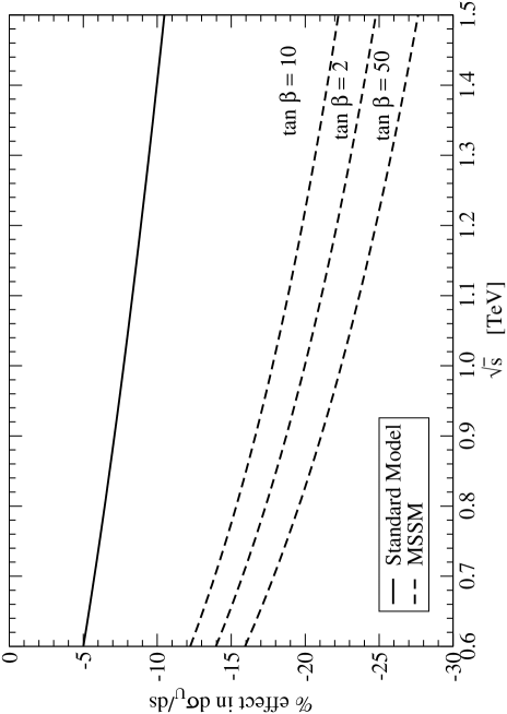
FIG. 2.: Relative one loop corrections to the unpolarized cross section $d\sigma_{U}/ds$. More precisely, we show the difference $d\sigma_{U}^{1\ loop}/ds-d\sigma_{U}^{Born}/ds$ divided by $d\sigma_{U}^{Born}/ds$. The plot shows the effect in the Standard Model and in the MSSM with three reference values of $\tan\beta=2,10,50$.

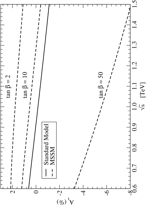
FIG. 3.: One loop value of the top quark polarization asymmetry $A_{t}$. The plot shows the effect in the Standard Model and in the MSSM with three reference values of $\tan\beta=2,10,50$.

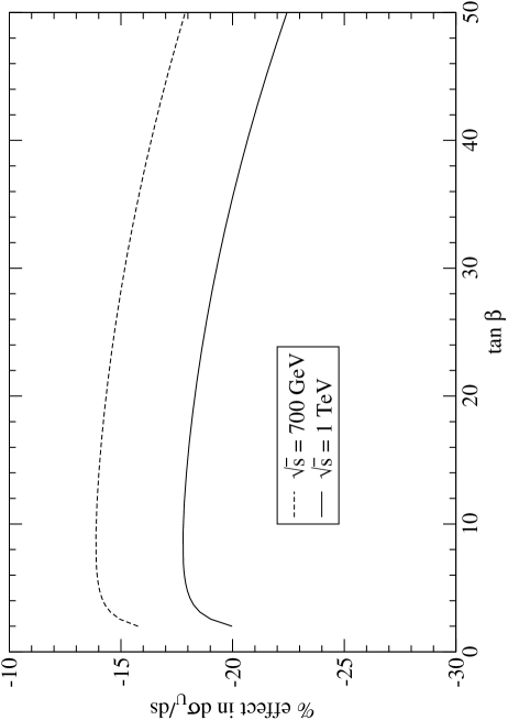
FIG. 4.: Relative one loop corrections to the unpolarized cross section $d\sigma_{U}/ds$. As in Fig. 2, we show the ratio $(d\sigma_{U}^{1\ loop}/ds-d\sigma_{U}^{Born}/ds)/d\sigma_{U}^{Born}/ds$. The plot shows the effect in the MSSM as a function of $\tan\beta$ at two reference values of $\sqrt{s}=700,1000$ GeV.

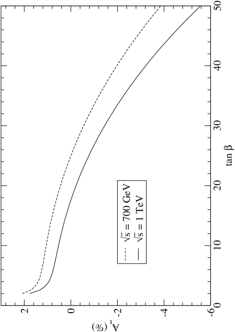
FIG. 5.: One loop expression of the top quark polarization asymmetry $A_{t}$. The plot shows the effect in the MSSM as a function of $\tan\beta$ at two reference values of $\sqrt{s}=700,1000$ GeV.

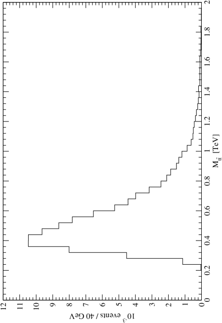
FIG. 6.: Event distribution as function of $M_{t\bar{t}}$ in the Standard Model. The events are obtained from semileptonic top decay corresponding to 5 fb^-1 of collected data (half a year at luminosity $10^{33}{\rm cm}^{-2}{\rm s}^{-1}$).

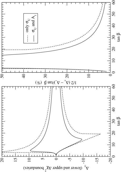
FIG. 7.: Results from the $\chi^{2}$ analysis of the $\tan\beta$ dependence of the two considered distributions. For each hypothetical true value of $\tan\beta$, the figures show the $\Delta\chi^{2}=1$ boundaries $\tan\beta+\Delta_{\pm}$ and the corresponding relative error defined as $\frac{1}{2}(\Delta_{+}-\Delta-)/\tan\beta$. The dashed and solid lines are obtained by exploiting the unpolarized cross section alone or the combination of it with the polarization asymmetry.

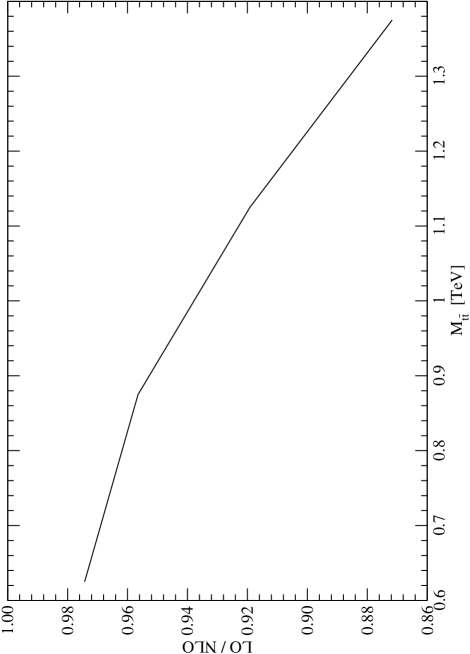
FIG. 8.: Ratio of normalised NLO and LO predictions of the distribution of $M_{tt}$, i.e. $[M_{tt}/\sum M_{tt}]/[\sqrt{s}/\sum\sqrt{s}]$, as determined from the MC@NLO and Herwig programs. This ratio is only sensitive to the difference in shape of the two predictions.

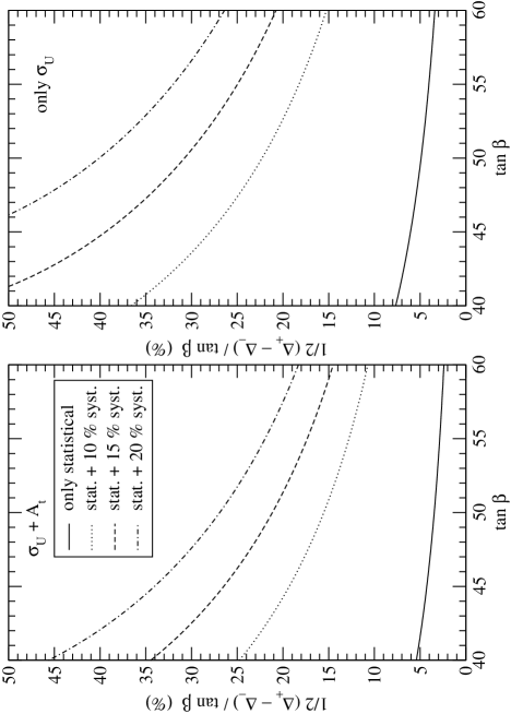
FIG. 9.: This figure shows the same analysis described in Fig. (7). However, we now take into account an energy independent fixed systematic error of 10, 15 or 20 %. The curves on the left are obtained by including in the analysis both the unpolarized cross section and the polarization asymmetry $A_{t}$. The curves on the right do not use $A_{t}$.

REFERENCES

- [1] ”Top quark Physics”, M. Beneke et al, CERN-TH-2000-004, Proc. of the workshop on Standard Model physics (and more) at the LHC; editors G. Altarelli and M. L. Mangano, Geneva 2000, pag. 419; ATLAS Detector and Physics Performance Technical Design Report, LHCC 99-14/15.
- [2] W. Hollik, W.M. Mösle and D. Wackeroth, Nucl.Phys. B516, 19 (1998).
- [3] C. Kao and D. Wackeroth, Phys. Rev. D61, 055009 (2000); hep-ph/9902202.
- [4] M. Beccaria, F.M. Renard and C. Verzegnassi, Phys. Rev. D69, 113004 (2004).
- [5] M. Beccaria, F. M. Renard and C. Verzegnassi, Phys. Rev. D64, 073008 (2001). M. Beccaria, M. Melles, F. M. Renard and C. Verzegnassi, Phys.Rev.D65, 093007 (2002). M. Beccaria, F.M. Renard and C. Verzegnassi, Phys. Rev. D63, 095010 (2001); Phys.Rev.D63, 053013 (2001); M. Beccaria, M. Melles, F.M. Renard, S. Trimarchi, C. Verzegnassi, Int.Jour.Mod.Phys.A18,5069 (2003).
- [6] M. Beccaria, F.M. Renard, S. Trimarchi, C. Verzegnassi, Phys. Rev. D 68,035014 (2003).
- [7] see e.g. R.K. Ellis, W.J. Stirling and B.R. Webber, ”QCD and Colliders Physics”, Cambridge University Press, eds. T.Ericson and P.V. Landshoff (1996).
- [8] General information and updated numerical routines for parton distribution functions can be found on the www site http://durpdg.dur.ac.uk/hepdata/. The set we used is described in A.D. Martin, R.G. Roberts, W.J. Stirling, R.S. Thorne, “MRST partons and uncertainties”, contribution to XI International Workshop on Deep Inelastic Scattering, St. Petersburg, 23-27 April 2003, hep-ph/0307262.
- [9] E. Cogneras, Recherche de resonances ttbar avec le detecteur ATLAS, rapport de DEA, Universite’ Blaise Pascal de Clermont Ferrand II.
- [10] A. Datta, A. Djouadi, and J-L. Kneur, Phys. Lett. B509, 299 (2001); J. Gunion et al., ibid. 565, 42 (2003).
- [11] I. Borianovc et al, Top quark mass measurement with the ATLAS detector at LHC, SN-ATLAS-2004-040.
- [12] S. Frixione, B. Webber, Matching NLO QCD computations and parton shower simulations, JHEP06, 2002.
- [13] Pythia, T. Sjöstrand, P. Edén, C. Friberg, L. Lönnblad, G. Miu, S. Mrenna and E. Norrbin, Computer Phys. Commun. 135, 238 (2001) (LU TP 00-30, hep-ph/0010017).
- [14] Atlfast, a fast simulation package for ATLAS, E. Richter-Was, D. Froidevaux, L. Poggioli, ATL-PHYS-98-13.
- [15] M. Beccaria, S. Moretti, F.M. Renard, D. Ross, C. Verzegnassi, in preparation.