Bose-Einstein or HBT correlations
and the anomalous dimension of QCD

Abstract

The Bose-Einstein (or HBT) correlation functions are evaluated for the fractal structure of QCD jets. These correlation functions have a stretched exponential (or Lévy-stable) form. The anomalous dimension of QCD determines the Lévy index of stability, thus the running coupling constant of QCD becomes measurable with the help of two-particle Bose-Einstein correlation functions. These considerations are tested on NA22 and UA1 two-pion correlation data.

05.40.Fb, 13.85.Hd, 13.87.Ce, 25.75.-q, 25.75.Gz

1 Introduction

The study of fractal phenomena was introduced to high energy particle and nuclear physics by Bialas and Peschanski in ref. [1], see also ref.[2] for a review. In QCD, jets emit jets that emit additional jets and so on. The resulting fractal structure of QCD jets was explored with the help of a beautiful geometric picture in refs. [3, 4, 5]. These ideas were developed further by the Lund group in refs.  [6, 7, 8], by Dokshitzer and Dremin in ref. [9] as well as by Ochs and Woisek in refs. [10, 11]. Both theoretical and experimental aspects of the so-called intermittency or fractal structures in high energy physics were reviewed by De Wolf, Dremin and Kittel in ref. [12].

Bialas realized, that Bose-Einstein correlations and intermittency might be deeply connected [13]. The mathematical properties of Bose-Einstein correlation functions for Lévy stable (convolution invariant) sources were written up by three of us in refs. [14, 15]. Here we add a physical interpretation and show, that the fractal properties of QCD cascades can naturally be measured by the Lévy index of stability of Bose-Einstein correlations. Our analytical results are similar in spirit to the numerical investigations of Wilk and collaborators in ref. [16].

2 (Multi)fractal structure of the QCD jets

In this section we recapitulate earlier theoretical results of the Lund group,  [3, 4, 5, 6, 7, 8], that related the properties of QCD cascades to intermittency. These results are based on a beautiful geometric interpretation of the color dipole picture, and on an infrared stable measure on parton states related to hadronic multiplicity.

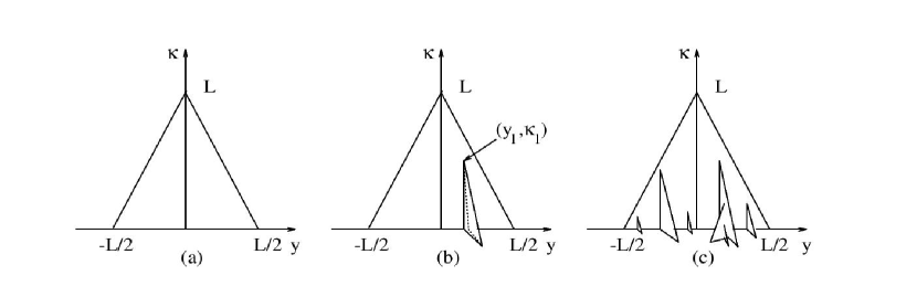
Figure 1: The phase-space of QCD jets in the $(y,\kappa)$ plane, where $\kappa=\log(k_{t}^{2})$. (a) The phase-space available for a gluon emitted by a high energy $q\overline{q}$ system is a triangular region in the $(y,\kappa)$ plane. (b) If one gluon is emitted at $(y_{1},\kappa_{1})$, the phase-space for a second (softer) gluon is given by the area of this folded surface. (c) The total gluonic phase-space can be described by this multifaceted fractal surface [3, 4, 5].

A high energy $q\overline{q}$ system radiates gluons according to the dipole formula

$$dn=\frac{3\alpha_{s}}{4\pi^{2}}\frac{dk_{\perp}^{2}}{k_{\perp}^{2}}dyd\phi,$$ (1)

hence the phase-space for the emission of a gluon is given by the relation

$$|y|\leq\frac{1}{2}\ln(s/k_{\perp}^{2}),$$ (2)

which corresponds to the triangular region in a $(y,\ln k_{\perp}^{2})$ diagram as shown in Fig. 1 (a). If two gluons are emitted, then the distribution of the hardest gluon is described by eq. (1). The distribution of the second, softer, gluon corresponds to two dipoles, the first is stretched between the quark and the first gluon, and the second between the first gluon and the anti-quark. The phase-space available for the second gluon corresponds to the folded surface in Fig. 1 (b), with the constraint $k_{\perp,2}^{2}<k_{\perp,1}^{2}$, as the first gluon is assumed to be the hardest one. This procedure can be generalized so that the emission of a third, still softer gluon corresponds to radiation from three color dipoles, with $n$ gluons emitted already the emission of the $(n+1)$-th gluon is given by a chain of $n+1$ dipoles. Thus, with many gluons, the gluonic phase-space can be represented by a multi-faceted surface as illustrated in Fig. 1 (c). Each gluon adds a fold to the surface, which increases the phase-space for softer gluons. (Note, that in this process the recoils are neglected, as is normal in leading log approximation). Due to its iterative nature, the process generates a Koch-type fractal curve at the base-line. The length of this base-line of the partonic structure on Figure 1.c is proportional to the particle multiplicity. This curve is longer, when studied with higher resolution: it is a fractal curve, embedded into the four-dimensional energy-momentum space, characterized by the fractal dimension

$$d_{f}=1+\sqrt{\frac{3\alpha_{s}}{2\pi}},$$ (3)

or one plus the anomalous dimension of QCD [3, 4, 5].

With the help of the Lund string fragmentation picture, this fractal in momentum space is mapped into a fractal in coordinate space, and the constant of conversion is the hadronic string tension, $\kappa\approx 1$ GeV/fm. This mapping does not change the fractal properties of the curve. The emission of softer and softer gluons corresponds to a smaller and smaller modification of this curve, as a gluon with a very small transverse mass creates a very small kink on the Lund string. Hence this process is infrared stable.

3 Bose-Einstein correlations for Lévy stable source distributions

Let us discuss here the stability of the particle emitting source in QCD, and consider the Bose-Einstein correlation functions for such sources. The two-particle Bose-Einstein correlation function is defined as the ratio of the two-particle invariant momentum distribution to the product of the single-particle invariant momentum distributions:

$$C_{2}({\mathbf{k}}_{1},{\mathbf{k}}_{2})=\frac{N_{2}({\mathbf{k}}_{1},{\mathbf{k}}_{2})}{N_{1}({\mathbf{k}}_{1})\,N_{1}({\mathbf{k}}_{2})}.$$ (4)

If long-range correlations can be neglected or corrected for, and if the short-range correlations are dominated by Bose-Einstein correlations, this two-particle Bose-Einstein correlation function is related to the Fourier-transformed source distribution. For clarity, let us consider the case of a one-dimensional, factorized coordinate and momentum space distribution,

$$S(x,k)=f(x)\,g(k).$$ (5)

In this case [14, 15], the Bose-Einstein correlation function is

$$C_{2}(k_{1},k_{2})=1+|\tilde{f}(q)|^{2},$$ (6)

where the Fourier transformed source density (often referred to as the characteristic function) and the relative momentum are defined as

$$\tilde{f}(q)=\int\mbox{\rm d}x\,\exp(iqx)\,f(x),\qquad\quad q=k_{1}-k_{2}.$$ (7)

Let us focus on the property of particle emission from QCD jets, that the fractal defining the particle emission is infrared stable: adding one more, very soft gluon does not change the resulting source distributions. Thus the source of particles is stable for convolution. The Bose-Einstein correlation functions for such particle emitting sources were evaluated recently by three of us, which we summarize in this section following refs. [14] and  [15].

For the case of the jets decaying to jets to jets and so on, the final position of a particle emission is given by a large number of position shifts, hence the distribution of the final position $x$ is obtained as a convolution,

$$x=\sum_{i=1}^{n}x_{i},\qquad\qquad f(x)=\int\Pi_{i=1}^{n}{\mbox{\rm d}}x_{i}\,\Pi_{j=1}^{n}f_{j}(x_{j})\,\delta(x-\sum_{k=1}^{n}x_{k}).$$ (8)

Various forms of the Central Limit Theorem state, that under certain conditions, the distribution of the sum of a large number of random variables converges (for $n\rightarrow\infty$) to a limit distribution. In case of “normal” elementary processes, that have finite means and variances, the limit distribution of their sum is a Gaussian. Stable distributions are precisely those limit distributions that can occur in Generalized Central Limit theorems. Their study was begun by the French mathematician Paul Lévy in the 1920’s. The stable distributions are frequently given in terms of their characteristic functions, as the Fourier transform of a convolution is a product of the Fourier-transforms,

$$\tilde{f}(q)=\prod_{i=1}^{n}\tilde{f}_{i}(q)$$ (9)

and limit distributions appear when the convolution of one more elementary process does not change the form of the limit distribution, but it results only in a modification of its location and scale parameters. The characteristic function of univariate and symmetric stable distributions is

$$\tilde{f}(q)=\exp\left(iq\delta-|\gamma q|^{\alpha}\right),$$ (10)

where the support of the density function $f(x)$ is $(-\infty,\infty)$. Deep mathematical results imply that the index of stability, $\alpha$, satisfies the inequality $0<\alpha\leq 2$, so that the source distribution be always positive. These Lévy distributions are indeed stable for convolutions, in the following sense:

$$\tilde{f}_{i}(q) = \exp\left(iq\delta_{i}-|\gamma_{i}q|^{\alpha}\right),\qquad\prod_{i=1}^{n}\tilde{f}_{i}(q)\,=\,\exp\left(iq\delta-|\gamma q|^{\alpha}\right),$$ (11)

$$\gamma^{\alpha} = \sum_{i=1}^{n}\gamma_{i}^{\alpha},\quad\qquad\qquad\qquad\delta\,=\,\sum_{i=1}^{n}\delta_{i}.$$ (12)

Thus the Bose-Einstein correlation functions for univariate, symmetric stable distributions (after a core-halo correction, and a re-scaling) read as

$$C(q;\alpha)=1+\lambda\exp\left(-|qR|^{\alpha}\right).$$ (13)

For the special value of $\alpha=2$ we obtain the well known Gaussian case. Refs. [14] and  [15] discuss further examples and details and generalize these results to three dimensional, hydrodynamically expanding, core-halo type sources as

$$C(q,K;\alpha)=1+\lambda(K)\exp\left(-|\sum_{i,j}q_{i}R_{ij}^{2}(K)q_{j}|^{\alpha/2}\right).$$ (14)

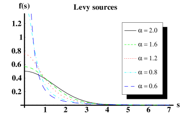
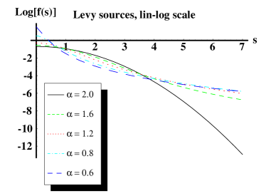
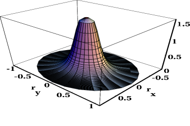
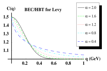
Figure 2: (a - top left) Source functions for univariate symmetric Lévy laws, as a function of the dimensionless variable $s=r/R$, on a linear-linear scale, for various values of the Lévy index of stability, $\alpha$. (b - top right) Same as (a), but on a linear-logarithmic plot. Note the power-law tails that decay in case of $\alpha<2$ for large values of $s$ as $f_{\alpha}(s)\propto s^{-1-\alpha}$. (c - bottom left) Source function for two-dimensional symmetric Lévy laws, for $\alpha=0.6$. (d - bottom right) Bose-Einstein correlation (or HBT) correlation functions for univariate symmetric Lévy laws, for a fixed scale parameter of $R=0.8$ fm and various values of the Lévy index of stability, $\alpha$.

Figure 2 (a) shows univariate symmetric Lévy source distributions. Figure 2 (b) illustrates, that values of the index of stability $\alpha$ are related to the tails of these distributions. If $\alpha<2$, for large values of $s=r/R$ the Lévy sources decay as $f_{\alpha}(s)\propto s^{-1-\alpha}$. Figure 2 (c) shows a two-dimensional symmetric Lévy stable source. Bose-Einstein correlation functions for Lévy stable source distributions are shown in Figure 2 (d) for various values of the index of stability $\alpha$, and for a constant value of the radius parameter $R$. These Bose-Einstein correlation functions are sensitive to the value of $\alpha$ not only in the small $Q<\hbar/R$ region, but are also in the “large” relative momentum region of $Q>\hbar/R$. Thus these correlations are sensitive to the structure of the particle emission in the region which is shaped by the jets.

A random walk, where the length of the steps is given by a Lévy distribution, and the direction of the steps is random, corresponds to a fractal curve, in physical terms it can be interpreted as the path of a test particle performing a generalized Brownian motion. This motion is referred to as anomalous diffusion and the probability that the test particle diffuses to distances $r$ greater than a certain value of $|s|$ is given by $P(r>|s|)\propto|s|^{-\alpha}$. This relation is valid for anomalous diffusion not only in one, but also in two and three dimensions. Thus the Lévy index of stability $\alpha$ is the fractal dimension of the trajectory of the corresponding anomalous diffusion [17]. When we apply this result to QCD, there are two key considerations.

First, if gluon radiation is neglected, the $q\overline{q}$ system hadronizes as a 1+1 dimensional hadronic string, which has no fractal structure. If the gluon emission is switched on, the emission of gluon $n$ from one of the $n$ dipoles corresponds to a step of an anomalous diffusion in the plane transverse to the given dipole. Hence the anomalous dimension of QCD equals to the Lévy index of stability of this anomalous diffusion,

$$\sqrt{\frac{3\alpha_{s}}{2\pi}}=\alpha_{\mbox{\tiny\rm L\'{e}vy}}.$$ (15)

Second, data on Bose-Einstein correlations are often determined in terms of the invariant momentum difference $Q_{\rm inv}=\sqrt{-(p_{1}-p_{2})^{2}}$. Bose-Einstein correlation functions that depend on this invariant momentum difference can be obtained within the framework of the so-called $\tau$-model. This model assumes a broad proper-time distribution, $H(\tau)$ and very strong correlations between coordinate and momentum in all directions, $x^{\mu}/\tau\propto p^{\mu}/m_{(t)}$. Hence $(x_{1}-x_{2})(p_{1}-p_{2})\propto\tau Q_{\rm inv}^{2}$, see refs. [18, 19] for details. In this case, the Bose-Einstein correlation function measures the Fourier-transformed proper-time distribution $\tilde{H}$ in the following, unusual manner:

$$C_{2}(Q_{\rm inv})\simeq 1+\lambda\,\mbox{\it Re}\,\tilde{H}^{2}\left(\frac{Q_{\rm inv}^{2}}{2m_{(t)}}\right),$$ (16)

where $m_{(t)}$ stands for the (transverse) mass of the pair for (two)- or more jet events. From this relation it follows, that $\alpha_{\mbox{\tiny\rm BEC}}=2\alpha_{\mbox{\tiny\rm L\'{e}vy}}$. Thus we find the following relationship between the strong coupling constant and the exponent of an invariant relative momentum dependent Bose-Einstein correlation function:

$$\alpha_{s}=\frac{\pi}{6}\alpha^{2}_{\mbox{\tiny\rm BEC}}.$$ (17)

4 Application to NA22 and UA1 data

In ref. [14] three of us have fitted the NA22 [20] and the UA1 data [21] on two-particle Bose-Einstein correlation functions with the Lévy stable form of eq.  (13). The results were summarized in Table 1 of that paper. Here we re-interpret the exponent of this fit with the help of eq. (17) and extract $\alpha_{s}$, the coupling constant of QCD, as given by Table 1 of this paper.

	NA22		UA1
Parameter	Value	Error	Value	Error
$\alpha_{\mbox{\tiny\rm BEC}}$ from ref. [14]	0.67	$\pm$ 0.07	0.49	$\pm$ 0.01
$\alpha_{s}$ from eq. (17)	0.24	$\pm$ 0.05	0.13	$\pm$ 0.01

Table 1: Converting the best Lévy fits to UA1 and NA22 two-particle correlations using the $\tau$-model converted with eq.(17) to values for the running QCD coupling constant $\alpha_{s}$.

5 Summary, conclusions

Using the picture of strongly correlated coordinate and momentum space distributions, we determined the (running of the) strong coupling constant from NA22 and UA1 two-pion Bose-Einstein correlation measurements.

References

- [1] A. Bialas and R. Peschanski, Nucl. Phys. B 273 (1986) 703.
- [2] A. Bialas, Nucl. Phys. A 525 (1991) 345.
- [3] P. Dahlqvist, B. Andersson and G. Gustafson, Nucl. Phys. B 328 (1989) 76.
- [4] G. Gustafson and A. Nilsson, Nucl. Phys. B 355 (1991) 106.
- [5] G. Gustafson, Proc Int. Workshop on Correlations and Multiparticle Production, Marburg, West Germany, May 14-16, 1990 (World Scientific, Singapore, 1991, eds. M. Plümer, S. Raha and R. M. Weiner)
- [6] G. Gustafson and A. Nilsson, Z. Phys. C 52 (1991) 533.
- [7] G. Gustafson, Nucl. Phys. B 392, 251 (1993).
- [8] B. Andersson, G. Gustafson, J. Samuelsson, Nucl. Phys. B 463 (1996) 217.
- [9] Y. L. Dokshitzer and I. M. Dremin, Nucl. Phys. B 402 (1993) 139.
- [10] W. Ochs and J. Wosiek, Phys. Lett. B 305 (1993) 144.
- [11] W. Ochs and J. Wosiek, Z. Phys. C 68 (1995) 269.
- [12] E. A. De Wolf, I. M. Dremin and W. Kittel, Phys. Rept. 270 (1996) 1
- [13] A. Bialas, Acta Phys. Polon. B 23 (1992) 561.
- [14] T. Csörgő, S. Hegyi and W. A. Zajc, Eur. Phys. J. C 36, 67 (2004)
- [15] T. Csörgő, S. Hegyi and W. A. Zajc, arXiv:nucl-th/0402035.
- [16] O. V. Utyuzh, G. Wilk and Z. Wlodarczyk, Phys. Rev. D 61, 034007 (2000).
- [17] V. Seshardi, B. J. West, Proc. Nat. Acad. Sci. USA 79 pp. 4501 - 4505 (1982)
- [18] T. Csörgő and J. Zimányi, Nucl. Phys. A 517 (1990) 588
- [19] T. Csörgő, in Proc. XXXII Int. Symp. Multipart. Dynamics [hep-ph/0301164]
- [20] N. M. Agababian et al. [EHS/NA22 Coll.], Z. Phys. C 59, 405 (1993).
- [21] N. Neumeister et al. [UA1-Min. Bias-Coll.], Z. Phys. C 60, 633 (1993).