Pentaquark resonances from collision times

Abstract

Having successfully explored the existing relations between the $S$-matrix and collision times in scattering reactions to study the conventional baryon and meson resonances, the method is now extended to the exotic sector. To be specific, the collision time in various partial waves of $K^{+}N$ elastic scattering is evaluated using phase shifts extracted from the $K^{+}N\rightarrow K^{+}N$ data as well as from model dependent $T$-matrix solutions. We find several pentaquark resonances including some low-lying ones around 1.5 to 1.6 GeV in the $P_{01}$, $P_{03}$ and $D_{03}$ partial waves of $K^{+}N$ elastic scattering.

1 Introduction

The discovery of the pion in 1947 followed by that of several other mesons and baryons, gave birth to a specialized branch in particle physics which involved the characterization of hadronic resonances. However, even after half a century’s experience in analyzing experimental data to infer on the existence of resonances we still come across examples where a resonance is confirmed by one type of analysis and is reported to be absent by another and history shows that this is especially true in the case of the pentaquark ($Z^{*}$) resonances. It is therefore important to examine the limitations of the various theoretical definitions used to extract information from data and then comment on the existence of the resonance. The pentaquark resonance, $\Theta^{+}(1540)$, found in several experiments[1] which followed its theoretical prediction[2] is one such recent example. In the present talk we try to shed some light on the controversy[3] of its existence using a somewhat forgotten but well-documented method of collision time or time delay in scattering. In fact, we identify several pentaquark resonances by evaluating the time delay in various partial waves of $K^{+}N$ elastic scattering using the available $K^{+}N\rightarrow K^{+}N$ data.

2 Collision time: From the fifties until now

Intuitively, one would expect that if a resonance is formed as an intermediate state in a scattering process (say $a+b\rightarrow R\rightarrow a+b$), then the scattered particles in the final state would emerge (alone from the fact that the resonance has a finite lifetime) later than in a non-resonant process $a+b\rightarrow a+b$. The resonant process would be “delayed” as compared to the non-resonant one. This relevance of the delay time or collision time in scattering processes to resonance physics was noticed back in the fifties by Eisenbud[4], Bohm[5] and Wigner[6]. Wigner considered a simple wave packet with the superposition of two frequencies to show that the amount of time by which an incoming particle in a scattering process got delayed due to interaction with the scattering centre is proportional to the energy derivative of the scattering phase shift, $\delta(E)$. For a wavepacket consisting of two terms with frequencies $\nu\pm\Delta\nu$, wave numbers $k\pm\Delta k$ and phase shifts $2(\delta\pm\Delta\delta)$, the incident and outgoing waves can be written as,

$$\Psi_{inc}=2v^{-1}[e^{i(kx+\nu t)}cos(x\Delta k+t\Delta\nu)]$$

and

$$\Psi_{out}=2v^{-1}[e^{i(kx-\nu t+2\delta)}cos(x\Delta k-t\Delta\nu+2\Delta\delta)]$$

where one can see that $\Psi_{inc}$ has a maximum when $x_{max}=-t(d\nu/dk)=-vt$, and represents a particle moving inwards at times $t<0$ whereas $\Psi_{out}$ has $x_{max}=vt-2d\delta/dk$ for a later time $t$. Thus the interaction has delayed the particle by an amount

$$\Delta t=2v^{-1}{d\delta\over dk}=2\hbar{d\delta\over dE}\,.$$ (1)

In the absence of interaction, obviously, $\delta=0$ and $d\delta/dk=0$ and there is no time delay. From this, Wigner concluded that close to resonances, where the incident particle is captured and retained for some time by the scattering centre, $d\delta/dk$ will assume large positive values. However, in the case of non-resonant scattering, the interaction can sometimes also speed up the scattering process resulting in a negative time delay or time advancement. The negative time delay cannot take arbitrarily large values and in fact Wigner put a limit from the principle of causality as,

$${d\delta\over dk}>-a$$

where $a$ is the radius of the scattering centre.

Eisenbud[4] defined a delay time matrix, $\mbox{\boldmath$\Delta$}{\bf t}$, in terms of the scattering matrix S, where a typical element of $\mbox{\boldmath$\Delta$}{\bf t}$,

$$\Delta t_{ij}=Re\big{[}-i\hbar(S_{ij})^{-1}{dS_{ij}\over dE}\big{]}\,,$$ (2)

gave the delay in the outgoing signal in the $j^{th}$ channel when the signal is injected in the $i^{th}$ channel. For an elastic scattering reaction, $i=j$ and one can easily see that using a phase shift formulation of the $S$-matrix, i.e. $S=e^{2i\delta}$ in the purely elastic case and $S=\eta e^{2i\delta}$ for elastic scattering in the presence of inelasticities, the above relation reduces simply to[7, 8]

$$\Delta t_{ii}=2\hbar{d\delta\over dE}\,.$$ (3)

Henceforth for simplicity, we shall drop the subscripts $ii$ and write $\Delta t$ whenever we refer to time delay in elastic scattering. Since the particle has probability $|S_{ij}|^{2}$ of emerging in the $j^{th}$ channel, the average time delay for a particle injected in the $i^{th}$ channel is given as,

$$\langle\,\Delta t_{i}\,\rangle_{av} = \sum_{j}\,S_{ij}^{*}S_{ij}\,\Delta t_{ij}\,$$ (4)

$$= \,Re\biggr{[}\,-i\hbar\,\sum_{j}S^{*}_{ij}\,{dS_{ij}\over dE}\biggr{]}\,.$$

Later on, Smith[9] constructed a lifetime matrix ${\bf Q}$, which was given in terms of the scattering matrix, ${\bf S}$ as,

$${\bf Q}=i\hbar\,{\bf S}\,{d{\bf S}^{{\dagger}}\over dE}\,.$$ (5)

He defined collision time to be the limit as $R\to\infty$, of the difference between the time the particles spend within a distance $R$ of each other (with interaction) and the time they would have spent there without interaction. The matrix elements of ${\bf Q}$ (which is hermitian) were given by,

$$Q_{ij} = \lim_{R\to\infty}[\int^{r<R}\Psi_{i}\Psi_{j}^{*}d\tau-R(v_{i}^{-1}\delta_{ij}+\sum_{k}S_{ik}v_{k}^{-1}S_{jk}^{*})]_{av}$$ (6)

$$= i\hbar\sum_{n}S_{in}\biggl{(}{dS_{jn}^{*}\over dE}\biggr{)}$$

where $S_{ik}$ is an element of ${\bf S}$ and $Q_{ij}$ is finite if the interaction vanishes rapidly at large $R$. One can now see that the average time delay for a collision beginning in the $i^{th}$ channel calculated using Eisenbud’s $\mbox{\boldmath$\Delta$}{\bf t}$ (Eq. 4 ) as above, is indeed the matrix element $Q_{ii}$ of the lifetime matrix. Smith concluded that when $Q_{ii}$’s are positive and large, we have a criterion for the existence of metastable states.

The interest in this concept continued in the sixties and Goldberger and Watson[10], using the concept of time interval in $S$-matrix theory found that

$$\Delta t=-i\hbar\,{d[lnS(E)]\over dE}\,.$$ (7)

Lippmann[11] even defined a time delay operator,

$$\mbox{\boldmath$\tau$}=-i\hbar\partial/\partial E\,,$$ (8)

the expectation value of which (using the phase shift formulation of the $S$-matrix) gave the time delay to be the same as in Eq. (3).

In the seventies, the time delay concept finally found a place in most books on scattering theory and quantum mechanics[12], where it is mentioned as a necessary condition for the existence of a resonance. However, in spite of being so well-known in literature as well as books, it was rarely used to characterize resonances until its recent application[7, 8] to meson and baryon resonances. Instead, mathematical definitions of a resonance have been used over the decades for its identification and characterization. The simple physical concept of time delay was somehow always overlooked in practice. In what follows, we now analyse the shortcomings of the various definitions or tools used to locate resonances.

3 What is a resonance?

A resonance is theoretically clearly defined as an unstable state characterized by different quantum numbers. However, to identify such a state when it has been produced, one needs to define a resonance in terms of theoretical quantities which can be extracted from data. In principle, if an unstable state is formed for example in a scattering process, then the various definitions should simply serve as complementary tools for its confirmation. However, it does often happen that a resonance extracted using one definition appears to be “missing” within another. Before discarding the existence of such missing resonances, it is important to take into account the limitations of the various definitions of a resonance. We shall discuss these below.

3.1 S-matrix poles

The most conventional method of locating a resonance involves assuming that whenever an unstable particle is formed, there exists a corresponding pole of the $S$-matrix on the unphysical sheet of the complex energy plane lying close to the real axis[12]. The experimental data is usually fitted with a model dependent $S$-matrix and resonances are identified by locating the poles. However, Calucci and co-workers[13] took a different point of view. In the case of a resonance $R$ formed in a two body elastic scattering process, $a+b\rightarrow R\rightarrow a+b$, a sharp peak in the cross section accompanied by a rapid variation of the phase shift through $\pi/2$ with positive derivative (essentially the condition for large positive time delay) was taken as the signal for the existence of a resonance. The authors then constructed $S$-matrices satisfying all requirements of analyticity, unitarity and threshold and asymptotic behaviour in energy such that a sharp isolated resonance is produced without an accompanying pole on the unphysical sheet. They also ensured the exponential decay of such a state. It is both interesting and relevant to note that while concluding that resonances can belong to a “no-pole category”[14], the authors stressed the need for high accuracy data in the case of the $Z^{*}$’s (the pentaquark resonances) whose dynamical origin might be questionable.

3.2 Cross section bumps, Argand diagrams and Speed Plots

Though the existence of a resonance usually produces a large bump in the cross sections, it was shown in a pedagogic article by Ohanian and Ginsburg[15] that a maximum of the scattering probability (i.e. cross section) cannot be taken as a sufficient condition for the existence of a resonance. Resonances can also be identified from anticlockwise loops in the Argand diagrams of the complex scattering amplitude; however, these alone cannot gaurantee the existence of a resonance[16]. Finally, the speed plot peaks, i.e. peaks in

$$SP(E)=\biggl{|}{dT\over dE}\biggr{|}\,,$$ (9)

where $T$ is the complex scattering transition matrix, can in fact be ambiguous due to being positive definite by definition[7].

Given the ambiguities associated with each of the techniques used to identify resonances, they should rather be used as complementary tools. We shall present the results of a time delay analysis of the $K^{+}N$ elastic scattering using the existing $K^{+}N\rightarrow K^{+}N$ data as well as the SP92[17] model dependent $T$-matrix solutions. However, before going over to the characterization of the $Z^{*}$ resonances through the time delay analysis, we give a brief review of the history of the identification of these pentaquark resonances. We will see that the old determinations of the pentaquarks were just as controversial as the most recently discovered $\Theta^{+}$.

4 Historical evidences of the $Z^{*}$’s

4.1 Earliest evidences

The search for the strangeness, $S=+1$ exotic baryons started back in the late fifties when Burrowes et al.[18] measured the Kaon-Nucleon total cross sections from 0.6 to 2 GeV centre of mass energy with the hope that the total cross sections might exhibit a resonance analogous to the pion-nucleon behaviour. Indeed, they found a peak in the total $K^{+}N$ cross sections around 1.8 GeV centre of mass energy. In 1966, Cool et al.[19] reported measurements of the $K^{+}p$ and $K^{+}d$ total cross sections with increased precision and a possible $Z^{*}$ with mass $M\sim 1.9$ GeV and width $\Gamma\sim 180$ MeV. These were followed by searches for the exotic baryons in photoproduction experiments. Tyson et al. performed experiments[20] for the photoproduction of negative K mesons where the excitation function for the $K^{-}$ yield in the reaction $\gamma+p\rightarrow K^{-}+Z^{*}$ was fitted by a three resonance formula in the missing mass range 1500 - 2500 MeV. The best fit masses and widths for the three resonances fitted were as follows: $M=1860^{+60}_{-20}$, $\Gamma\sim 150$ MeV; $M=2125\pm 25$ MeV, $\Gamma\sim 75$ MeV and $M=2280\pm 20$ MeV, $\Gamma\sim 80$ MeV. With the availability of the $K^{+}p$ data, energy dependent phase shift analyses were performed[21] and a resonance in the $P_{11}$ partial wave of $K^{+}p$ elastic scattering was reported (on the basis of Argand diagrams) around $M\sim 2$ GeV and $\Gamma\sim 220$ MeV.

4.2 Seventies and eighties

The seventies mostly saw the confirmation of the $Z^{*}$’s through several partial wave analyses. S. Kato et al.[22] obtained four possible solutions from a phase shift analysis of $K^{+}p$ elastic scattering and on the basis of Argand diagrams concluded on a possible mass of the $Z^{*}$ around 1.9 to 2 GeV and $\Gamma\sim 130-250$ MeV in the $P_{13}$ partial wave. This work was followed by two articles by Aaron et al.[23] which reported evidence for the $Z^{*}$’s in the $D_{03}$, $S_{01}$ and $P_{01}$ partial waves using Argand diagrams and speed plots. Arndt et al.[24] fitted the $K^{+}p$ data with a coupled-channel $K$-matrix parametrization and found a $P_{13}$ resonance pole at ($1.796-i101$) GeV. With so much support gathering in favour of the existence of these exotic baryons, the $Z^{*}$’s finally found a place in the Particle Data Group Compilation in 1982. In 1984, Keiji Hashimoto[25] performed a single-energy phase shift analysis of the data then available and reported $Z^{*}$ resonances in the $P_{13}$, $D_{03}$, $P_{11}$ and $D_{05}$ partial waves of $K^{+}$-nucleon scattering.

In 1982 appeared yet another partial wave analysis of the $K^{+}$-nucleon scattering data by Nakajima et al[26]. On the basis of the counterclockwise motion in Argand diagrams, they reported three resonances: $M=1.931$ GeV, $\Gamma=347$ MeV in $P_{13}$; $M=1.778$ GeV, $\Gamma=662$ MeV in $P_{01}$ and $M=1.907$ GeV, $\Gamma=291$ MeV in the $D_{03}$ partial wave. A prominent bump in the speed plot of the $P_{01}$ partial wave at $1540$ MeV was however ignored and not mentioned as a resonance due to lack of support from the Argand diagram.

In the late eighties and nineties, unfortunately, a general reluctance to accept the $Z^{*}$’s as genuine resonances or unstable pentaquark states started building up. Articles appeared in literature where the authors were often too careful and labeled the resonances in different ways as ‘doorways’, ‘pseudoresonances’, ‘resonance-like structures’, ‘complicated structures in the unphysical sheet’ etc. The main reason for such labeling was that the criteria applied to establish the $Z^{*}$’s were too stringent; sometimes more stringent than those applied for the conventional baryon resonances. Hence 1992 saw the last appearance of the $Z^{*}$ in the Particle Data Group Compilation with the remark, “It might take 20 years before the issue of the existence of the $Z^{*}$ resonances is settled”.

4.3 The year 2003

The interest in the pentaquark states was greatly revived[27] by the discovery of a narrow exotic state by different experimental groups around a mass of 1540 MeV[1]. The motivation for the first experiments came from a theoretical prediction[2] and this low lying $Z^{*}$ was renamed as $\Theta^{+}$. Before closing this section on the history of the $Z^{*}$’s, it is worth mentioning that just a little before the above experiments reported the $\Theta^{+}$, a time delay analysis[28] of the old $K^{+}N$ scattering data confirmed several penatquark states in the 1.8 GeV region and revealed some new pentaquark states around $1.5-1.6$ GeV in the $P_{01}$, $P_{13}$ and $D_{03}$ partial waves. In the next section, we shall discuss the results of this analysis.

A good account of the history of the theoretical progress in the search of the exotics (mesons as well as baryons) can also be found in an article by D. P. Roy[29].

5 Time delay in $K^{+}N$ elastic scattering

5.1 Energy dependent calculations

We shall first present the time delay distributions (as a function of energy) using model dependent solutions of the $T$-matrix. Replacing $S=1+2iT$ in Eq. (2), the time delay in elastic scattering, in terms of the $T$-matrix[28] can be obtained from:

$$S^{*}_{ii}S_{ii}\,\Delta t_{ii}=2\hbar\biggl{[}{dT^{R}_{ii}\over dE}+2T^{R}_{ii}{dT^{I}_{ii}\over dE}-2T^{I}_{ii}{dT^{R}_{ii}\over dE}\biggr{]}$$ (10)

where $T$ contains the information of resonant and non-resonant scattering and is complex ($T=T^{R}+iT^{I}$). As can be seen in Fig. 1, in addition to the resonances around 1.8 GeV, we find some low-lying ones around 1.5-1.6 GeV. Table I shows that the time delay peak positions around 1.8 GeV agree with the pole positions obtained from the same $T$-matrix. However, the low-lying ones do not correspond to any poles. These peaks could possibly be considered as realistic examples of the no-pole category of resonances[14] mentioned in the previous section. However, it cannot be doubted that the resonances around $1.5$ GeV found using time delay have something in common with the recently found peaks in the experimental cross sections around $1.54$ GeV. At this point we note again that a speed plot peak at 1.54 GeV in the $P_{01}$ partial wave of $K^{+}N$ elastic scattering was already noted by Nakajima et al.[26]. However, due to lack of support from Argand diagrams they did not mention it as a pentaquark resonance.

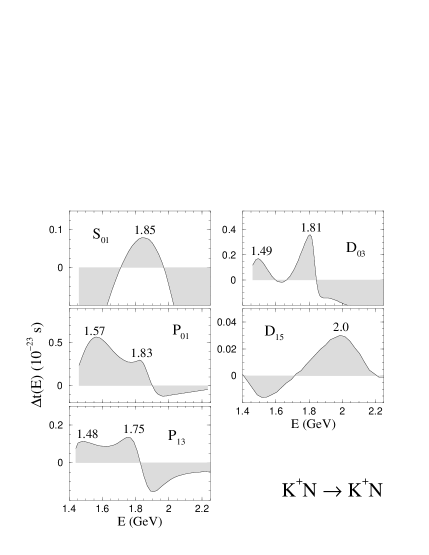
Figure 1: Time delay in various partial waves of $K^{+}N\rightarrow K^{+}N$ elastic scattering, evaluated from the SP92 $T$-matrix solutions.

Comparison of time delay peaks with pole values Partial wave SP92 pole position (GeV) Position of time delay peak $S_{01}$ - 1.85 $P_{01}$ - 1.57 1.831 - $i$95 1.83 $P_{13}$ - 1.48 1.811 - $i$118 1.75 $D_{03}$ - 1.49 1.788 - $i$170 1.81 $D_{15}$ 2.074 - $i$253 2.0

5.2 Pentaquark resonances from single energy values of $K^{+}N$ phase shifts

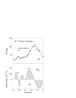
Figure 2: Time delay in the $D_{03}$ partial wave of $K^{+}N\rightarrow K^{+}N$ elastic scattering, evaluated from a fit (solid line in [a]) to the single energy values of the phase shift.

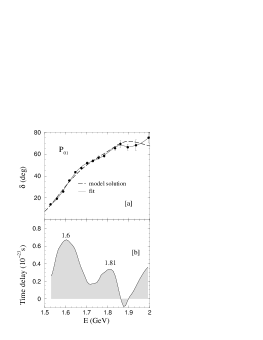
Figure 3: Same as Fig. 2, but for the $P_{01}$ partial wave.

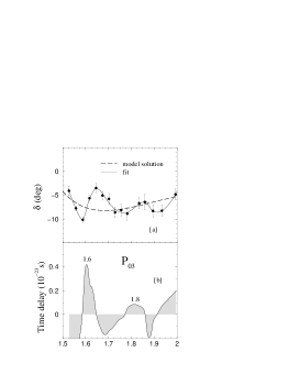
Figure 4: Same as Fig. 2, but for the $P_{03}$ partial wave.

Being motivated by our earlier experience with the meson and unflavoured baryon resonances[8], where small fluctuations in the single energy values of the phase shifts gave rise to time delay peaks corresponding to lesser established resonances, we decided to perform a time delay analysis of the single energy values of phase shifts in $K^{+}N$ elastic scattering too[28]. In Figs. 2, 3 and 4 we show the time delay distributions obtained from fits to the single energy values of the phase shifts. It is interesting to note a peak at 1.545 GeV in the $D_{03}$ partial wave which comes very close to the discovery of the $\Theta^{+}$ from recent cross section data. The peak at 1.64 GeV agrees with some of the predictions[30] of a $J^{P}=3/2^{+}$, $D_{03}$ partner of the $\Theta$(1540). In Figs. 3 and 4 we see that the resonances occur at exactly the same positions, namely, 1.6 and 1.8 GeV in the case of the $P_{01}$ and $P_{03}$ partial waves which are $J=1/2,3/2$ partners. The $J=3/2$ partners of the $\Theta^{+}$ have also been predicted[31] to lie in the region from 1.4 to 1.7 GeV. An interesting discussion on the possible spin and parity of the $\Theta^{+}$ by examining the two kaon photoproduction cross sections can be found in Ref.[33].

In closing, we note that the three peaks, namely, 1.545 in the $D_{03}$ and 1.6 and 1.8 GeV in the $P_{01}$ and $P_{03}$ partial waves are in very good agreement with the experimental values[32], 1.545$\pm$.012, 1.612$\pm$.01 and 1.821$\pm$.11 GeV of the resonant structures in the $pK_{s}^{0}$ invariant mass spectrum. We can then identify the time delay peak in the $D_{03}$ partial wave to be the $\Theta^{+}$. We summarize the findings in literature along with the resonances found using time delay in Table 2.

Determination of pentaquark resonances from different techniques in literature Partial Time delay Time delay Poles Argand wave (from fits) (SP92) diagrams $S_{01}$ 1.74 1.71[34] 1.85 1.85[17] 1.85[23] $P_{01}$ 1.6 1.57 1.81 1.83 1.83[17] 1.85[23] 1.78[26] $P_{03}$ 1.6 1.8 $P_{13}$ 1.6 1.5 1.75 1.75 1.81[17] 1.92 1.93[26] 1.9-2.0[22] $D_{03}$ 1.545 1.49 1.64 1.77 1.81 1.79[17] 1.85[23] 1.91[26] $D_{15}$ 2.0 2.0 2.1[17]

Note: The focus of this talk has been on the use of the time delay method for identifying pentaquark resonances. Hence we have not quoted all possible references on pentaquarks/exotics which appeared recently.

References

- [1] T. Nakano et al., Phys. Rev. Lett. 91, 012002 (2003); S. Stepanyan et al., Phys. Rev. Lett. 91, 252001 (2003); V. Kubarovsky et al., Phys. Rev. Lett. 92, 032001 (2004) Erratum-ibid. 92, 049902 (2004); V. V. Barmin et al., Phys. Atom. Nucl. 66, 1715 (2003), Yad. Fiz. 66, 1763 (2003), hep-ex/0304040; J. Barth et al., Phys. Lett. B572, 127 (2003); A. E. Asratyan, A. G. Dolgolenko and M. A. Kubantsev, hep-ex/0309042; A. Airapetian et al., Phys. Lett. B 585, 213 (2004); A. Aleev et al., hep-ex/0401024; S. V. Chekanov et al., hep-ex/0404007.
- [2] D. Diakonov, V. Petrov and M. Polyakov, Z. Phys. A 359, 305 (1997).
- [3] M. Praszalowicz, “Exotic Challenges”, this workshop; hep-ph/0410241; for a review on models, see also, Klaus Goeke, Hyun-Chul Kim, M. Praszalowicz and Ghil-Seok Yang, PNU-NTG-10-2004, hep-ph/0411195.
- [4] L. Eisenbud, Dissertation, Princeton, unpublished (June 1948).
- [5] D. Bohm, Quantum theory, New York: Prentice Hall, pp. 257-261 (1951).
- [6] E. P. Wigner, Phys. Rev. 98, 145 (1955).
- [7] N. G. Kelkar, J. Phys. G: Nucl. Part. Phys. 29, L1 (2003), hep-ph/0205188.
- [8] N. G. Kelkar, M. Nowakowski and K. P. Khemchandani, Nucl. Phys. A724, 357 (2003), hep-ph/0307184; M. Nowakowski and N. G. Kelkar, these proceedings, hep-ph/0411317; N. G. Kelkar, M. Nowakowski, K. P. Khemchandani and S. R. Jain, Nucl. Phys. A730, 121 (2004), hep-ph/0208197.
- [9] F. T. Smith, Phys. Rev. 118, 349 (1960).
- [10] M. L. Goldberger and K. M. Watson, Phys. Rev. 127, 2284 (1962).
- [11] B. A. Lippmann, Phys. Rev. 151, 1023 (1966).
- [12] M. L. Goldberger and K. M. Watson, Collision theory, Wiley, New York (1964); C. J. Joachain, Quantum Collision theory, North Holland, Amsterdam (1975); J. R. Taylor, Scattering theory, Wiley, New York (1972); B. H. Bransden and R. G. Moorhouse, The Pion-Nucleon System, Princeton University Press, NJ (1973).
- [13] G. Calucci, L. Fonda and G. C. Ghirardi, Phys. Rev. 166, 1719 (1968); G. Calucci and G. C. Ghirardi, Phys. Rev. 169, 1339 (1968).
- [14] L. Fonda, G. C. Ghirardi and G. L. Shaw, Phys. Rev. D8, 353 (1973).
- [15] H. Ohanian and C. G. Ginsburg, Am. J. Phys. 42, 310 (1974).
- [16] N. Masuda, Phys. Rev. D1, 2565 (1970); P. D. B. Collins, R. C. Johnson and G. G. Ross, Phys. Rev. 176, 1952 (1968).
- [17] J. S. Hyslop, R. A. Arndt, L. D. Roper and R. L. Workman, Phys. Rev. D46, 961 (1992).
- [18] H. C. Burrowes et al., Phys. Rev. Lett. 2, 117 (1959).
- [19] R. L. Cool et al., Phys. Rev. Lett. 17, 102 (1966).
- [20] J. Tyson et al., Phys. Rev. Lett. 19, 255 (1967).
- [21] A. T. Lea, B. R. Martin and G. C. Oades, Phys. Lett. 23, 380 (1966); B. R. Martin, Phys. Rev. Lett. 21, 1286 (1968).
- [22] S. Kato et al., Phys. Rev. Lett. 24, 615 (1971).
- [23] R. Aaron et al., Phys. Rev. D7, 1401 (1973); R. Aaron, R. D. Amado and R. R. Silbar, Phys. Rev. Lett. 26, 407 (1971).
- [24] R. A. Arndt and L. D. Roper, Phys. Rev. D 18, 3278 (1978); R. A. Arndt, R. H. Hackman and L. David Roper, Phys. Rev. Lett. 33, 987 (1974).
- [25] Keiji Hashimoto, Phys. Rev. C29, 1377 (1984).
- [26] K. Nakajima et al., Phys. Lett. B112, 80 (1982).
- [27] Jia-lun Ping, Di Qing, Fan Wang and T. Goldman, Phys. Lett. B602, 197 (2004), hep-ph/0408176; Fan Wang, Jia-lun Ping, Di Qing, T. Goldman, nucl-th/0406036; Carl E. Carlson, Christopher D. Carone, Herry J. Kwee, Vahagn Nazaryan, Phys. Rev. D70, 037501 (2004), hep-ph/0312325; ibid Phys. Lett. B579, 52 (2004), hep-ph/0310038; ibid Phys. Lett. B573, 101 (2003), hep-ph/0307396; S.I. Nam, A. Hosaka, H.C. Kim, Phys. Lett. B579, 43 (2004), hep-ph/0308313; Felipe J. Llanes-Estrada, eConf C0309101:FRWP011,2003, hep-ph/0311235.
- [28] N. G. Kelkar, M. Nowakowski and K. P. Khemchandani, J. Phys. G: Nucl. Part. Phys. 29, 1001 (2003), hep-ph/0307134; ibid, Mod. Phys. Lett. A, (2004), nucl-th/0405008.
- [29] D. P. Roy, J. Phys. G30, R113 (2004), hep-ph/0311207; for an early theoretical prediction of exotics including pentaquarks, see D. P. Roy and M. Suzuki, Phys. Lett. B28, 558 (1969).
- [30] B. K. Jennings and K. Maltman, Phys. Rev. D69, 094020 (2004); D. Akers, hep-ph/0403142.
- [31] L. Ya. Glozman, Phys. Lett. B575, 18 (2003); J. J. Dudek and F. E. Close, Phys. Lett. B583, 278 (2004).
- [32] P. Zh. Aslanyan, V. N. Emelyanenko and G. G. Rikhkvitzkaya, hep-ex/0403044.
- [33] W. Roberts, “A phenomenological Lagrangian approach to two kaon photoproduction and pentaquark searches”; nucl-th/0408034.
- [34] C. Roiesnol, Phys. Rev. D 20, 1646 (1979).