VECTOR AND AXIAL-VECTOR CURRENT CORRELATORS WITHIN THE INSTANTON MODEL OF QCD VACUUM.

Abstract

The pion electric polarizability, $\alpha^{E}_{\pi^{\pm}}$, the leading order hadronic contribution to the muon anomalous magnetic moment, $a_{\mu}^{\mathrm{hvp}\left(1\right)}$, and the ratio of the difference to the sum of vector and axial-vector correlators, $(V-A)/(V+A)$, are found within the instanton model of QCD vacuum. The results are compared with phenomenological estimates of these quantities following from the ALEPH and OPAL data on vector and axial-vector spectral densities.

In the chiral limit, where the masses of $u$, $d$, $s$ light quarks are set to zero, the vector ($V$) and axial-vector ($A$) current-current correlation functions in the momentum space (with $-q^{2}\equiv Q^{2}\geq 0$) are defined as

$$\Pi_{\mu\nu}^{J,ab}(q) = i\int d^{4}x~{}e^{iqx}\Pi_{\mu\nu}^{J,ab}(x)=\,\left(q_{\mu}q_{\nu}-g_{\mu\nu}q^{2}\right)\Pi_{J}(Q^{2})\delta^{ab},$$ (1)

$$\qquad\Pi_{\mu\nu}^{J,ab}(x) = \langle 0\left|T\left\{J_{\mu}^{a}(x)J_{\nu}^{b}(0)^{\dagger}\right\}\right|0\rangle,$$

where the QCD $V$ and $A$ currents are $J_{\mu}^{a}=\overline{q}\gamma_{\mu}\frac{\lambda^{a}}{\sqrt{2}}q,\ J_{\mu}^{5a}=\overline{q}\gamma_{\mu}\gamma_{5}\frac{\lambda^{a}}{\sqrt{2}}q,$ and $\lambda^{a}$ are Gell-Mann matrices $\left(\mathrm{tr}\lambda^{a}\lambda^{b}=2\delta^{ab}\right)$ in flavor space. The momentum-space two-point correlation functions obey (suitably subtracted) dispersion relations,

$$\Pi_{J}(Q^{2})=\int_{0}^{\infty}\frac{ds}{s+Q^{2}}\frac{1}{\pi}\mathrm{Im}\Pi_{J}(s),$$ (2)

where the imaginary parts of the correlators determine the spectral functions $\rho_{J}(s)=4\pi{\mathrm{Im}}\Pi_{J}(s+i0)$ measured by ALEPH [1] and OPAL [2].

In the instanton liquid model (ILM) gauged by interaction with external vector and axial-vector fields [3] the correlators in the chiral limit have transverse character [4, 5]

$$\Pi_{\mu\nu}^{J}\left(Q^{2}\right)=\left(g_{\mu\nu}-\frac{q^{\mu}q^{\nu}}{q^{2}}\right)\Pi_{J}^{\mathrm{ILM}}\left(Q^{2}\right),$$ (3)

and the dominant contribution to the correlators is given by the dynamical quark loop which was found in [4, 6] with the result for the vector current

$$\Pi_{V}^{Q\mathrm{Loop}}\left(Q^{2}\right)=\frac{4N_{c}}{Q^{2}}\int\frac{d^{4}k}{\left(2\pi\right)^{4}}\frac{1}{D_{+}D_{-}}\left\{M_{+}M_{-}+\left[k_{+}k_{-}-\frac{2}{3}k_{\perp}^{2}\right]_{ren}\right.$$

$$+ \left.\frac{4}{3}k_{\perp}^{2}\left[\left(M^{\left(1\right)}\left(k_{+},k_{-}\right)\right)^{2}\left(k_{+}k_{-}-M_{+}M_{-}\right)-\left(M^{2}\left(k_{+},k_{-}\right)\right)^{\left(1\right)}\right]\right\}+$$

$$+ \frac{8N_{c}}{Q^{2}}\int\frac{d^{4}k}{\left(2\pi\right)^{4}}\frac{M\left(k\right)}{D\left(k\right)}\left[M^{\prime}\left(k\right)-\frac{4}{3}k_{\perp}^{2}M^{\left(2\right)}\left(k,k+Q,k\right)\right],$$

where the notations $k_{\pm}=k\pm Q/2,k_{\perp}^{2}=k_{+}k_{-}-\frac{\left(k_{+}q\right)\left(k_{-}q\right)}{q^{2}},D\left(k\right)=k^{2}+M^{2}(k),$ and $M_{\pm}=M(k_{\pm}),\ D_{\pm}=D(k_{\pm})$ are used. We also introduce the finite-difference derivatives defined for an arbitrary function $F\left(k\right)$ as

$$F^{(1)}(k,k^{\prime})=\frac{F(k^{\prime})-F(k)}{k^{\prime 2}-k^{2}},\qquad F^{(2)}\left(k,k^{\prime},k^{\prime\prime}\right)=\frac{F^{(1)}(k,k^{\prime\prime})-F^{(1)}(k,k^{\prime})}{k^{\prime\prime 2}-k^{\prime 2}}.$$ (5)

The difference of the $V$ and $A$ correlators is free from any perturbative corrections for massless quarks and very sensitive to the spontaneous breaking of chiral symmetry. The model calculations of the chirality flip $V-A$ combination provides

$$\Pi_{V-A}^{Q\mathrm{Loop}}\left(Q^{2}\right)=-\frac{4N_{c}}{Q^{2}}\int\frac{d^{4}k}{\left(2\pi\right)^{4}}\frac{1}{D_{+}D_{-}}\left\{M_{+}M_{-}+\frac{4}{3}k_{\perp}^{2}\cdot\right.$$ (6)

$$\left.\left[-\sqrt{M_{+}M_{-}}M^{\left(1\right)}\left(k_{+},k_{-}\right)+\left(\sqrt{M}^{\left(1\right)}\left(k_{+},k_{-}\right)\right)^{2}\left(\sqrt{M_{+}}k_{+}+\sqrt{M_{-}}k_{-}\right)^{2}\right]\right\}.$$

Vice versa, $V$ and $A$ correlators are separately dominated by perturbative massless quark loop diagram in the high momenta region. In the model calculations this dominance is reproduced because in the chiral limit the dynamical quark mass generated in the instanton vacuum, $M(k)$, vanishes at large virtualities $k^{2}$.

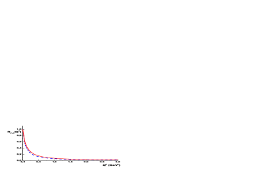
Figure 1: Normalized $V-A$ correlation function Eq. (13) obtained from the model (solid) and reconstructed from the ALEPH experimental spectral functions with next-to-leading accuracy in $\alpha_{s}$ (dashed).

With help of the Das-Mathur-Okubo (DMO) sum rule it is possible to estimate the electric polarizability of the charged pions by using the Gerasimov relation

$$\alpha^{E}_{\pi^{\pm}}=\frac{\alpha}{m_{\pi}}\left[\frac{\left\langle r_{\pi}^{2}\right\rangle}{3}-\frac{I_{DMO}}{f_{\pi}^{2}}\right],$$ (7)

where $I_{DMO}$ is the integral corresponding to the DMO sum rule

$$I_{DMO}=\frac{1}{4\pi^{2}}\int_{0}^{\infty}\frac{ds}{s}\left[\rho_{V}\left(s\right)-\rho_{A}\left(s\right)\right]=\left.\frac{\partial}{\partial Q^{2}}\left[Q^{2}\Pi_{V-A}\left(Q^{2}\right)\right]\right|_{Q^{2}\rightarrow 0}.$$ (8)

From (7) with values of charged pion radius and $I_{DMO}$ obtained from the model (see for further details [6, 7]) one finds the value

$$\left[\alpha^{E}_{\pi^{\pm}}\right]_{\mathrm{model}}=2.9\cdot 10^{-4}\mathrm{fm}^{3},$$ (9)

which is close to experimental numbers $\left[\alpha_{\pi^{\pm}}^{E}\right]_{\mathrm{exp}}^{\mathrm{OPAL}}=2.71(88)\cdot 10^{-4}\mathrm{~{}fm}^{3}$ [2] and [8] $\left[\alpha_{\pi^{\pm}}^{E}\right]_{\mathrm{exp}}^{\mathrm{PIBETA}}=\left\{\begin{array}[c]{l}2.68(9)\cdot 10^{-4}\mathrm{~{}fm}^{3}\qquad\mathrm{{full\ data\ set},}\\ 2.90(9)\cdot 10^{-4}\mathrm{~{}fm}^{3}\qquad\mathrm{kinematically\ restricted\ data\ set}.\end{array}\right.$ New precise results on pion and kaon polarizabilities are expected from COMPASS [9].

The leading order hadronic vacuum contribution to the lepton anomalous magnetic moment is given by

$$a_{\mu}^{\mathrm{hvp}\left(1\right)}=-\frac{2}{3}\alpha^{2}\int_{0}^{1}dx\left(1-x\right)\bar{\Pi}_{V}\left(\frac{x^{2}}{1-x}m_{l}^{2}\right),$$ (10)

where $\bar{\Pi}_{V}(Q^{2})=\Pi_{V}(Q^{2})-\Pi_{V}(0)$, $m_{l}$ is the lepton mass, and the charge factor $2/3$ is taken into account. One gets the model estimate

$$[a_{\mu}^{\mathrm{hvp}\left(1\right)}]_{\mathrm{model}}=6.2\left(0.4\right)\cdot 10^{-8}$$ (11)

which is in a reasonable agreement with the phenomenological numbers, found from precise determination of the low energy tail of the total $e^{+}e^{-}\rightarrow$ hadrons and $\tau$ lepton decays cross-sections[10]

$$[a_{\mu}^{\mathrm{hvp}\left(1\right)}]_{\mathrm{exp}}=\left\{\begin{array}[l]{l}6.934(88)\cdot 10^{-8},\qquad e^{+}e^{-},\\ 7.018(90)\cdot 10^{-8},\qquad\tau.\end{array}\right.$$ (12)

As by product we estimate also the anomalous magnetic moment of the $\tau$ lepton as [6] $[a_{\tau}^{\mathrm{hvp}\left(1\right)}]_{\mathrm{model}}=3.1\left(0.2\right)\cdot 10^{-6}.$

The ratio of correlators

$$R_{V,A}(Q^{2})=\frac{\bar{\Pi}_{V-A}\left(Q^{2}\right)}{\bar{\Pi}_{V-A}\left(Q^{2}\right)-2\bar{\Pi}_{V}\left(Q^{2}\right)}$$ (13)

characterizes the chirality transfer in dependence of passing virtuality. In (13) the vector correlator $\bar{\Pi}_{V}\left(Q^{2}\right)$ is defined above and the axial-vector correlator is defined with kinematical pole removed: $\bar{\Pi}_{V-A}(Q^{2})=\Pi_{V-A}(Q^{2})+f^{2}_{\pi}/Q^{2}$. This pole is not visible in experiment and difficult for detection on the lattice. From general grounds one expects that this ratio is unit at zero virtuality, and it goes to zero at large virtualities where perturbative dynamics dominates. In Fig. 1 we present the ratio of correlators, $R_{V,A}$, reconstructed from ALEPH spectral data.

The region of intermediate momentum transfer provides nontrivial transition between low energy dynamics described in terms of chiral symmetry structures and high energy dynamics with relevant operator product expansion language. The problems of standard approaches are the rapid growth of independent operator structures with less sensitivity of their experimental determination when moving beyond the applicability region. Moreover, there is a problem to define an energetic scale at which the standard expansions begin to work. These problems can be overcome with the aid of the instanton model of QCD vacuum. New data from ALEPH and OPAL on inclusive hadronic $\tau$ lepton decays are very helpful in study of current correlators, one of the simplest objects, at intermediate momentum transfer.