Scattering solutions of the spinless Salpeter equation

Abstract

A method to compute the scattering solutions of a spinless Salpeter equation (or a Schrödinger equation) with a central interaction is presented. This method relies on the 3-dimensional Fourier grid Hamiltonian method used to compute bound states. It requires only the evaluation of the potential at equally spaced grid points and yields the radial part of the scattering solution at the same grid points. It can be easily extended to the case of coupled channel equations and to the case of non-local interactions.

I Introduction

Numerous techniques have been developed to compute the scattering solutions of a Schrödinger equation. Simple Runge-Kutta methods can be performed in the case of a local potential, and discretization of the integration domain can be used for a non-local interaction pres92 . All these techniques can be used because the kinetic energy operator can be expressed in terms of a derivative operator. This is no longer true in the case of a spinless Salpeter equation for which the kinetic energy is a complicated square-root operator.

In a previous paper brau97a , we have developed a method to compute the eigenvalues of a spinless Salpeter equation. This method relies on the fact that the kinetic energy operator is best represented in momentum space, while the potential energy is generally given in coordinate space. It requires only the evaluation of the potential at equally spaced grid points, and yields directly the amplitude of the solution at the same grid points. This method is derived from the Fourier grid Hamiltonian method mars89 ; bali91 developed to compute the solution of the one-dimensional Schrödinger equation, and consequently was called the 3-dimensional Fourier grid Hamiltonian method. It appears very accurate and simple to handle.

In this paper, we show that 3-dimensional Fourier grid Hamiltonian method can be used to compute the scattering solutions of a spinless Salpeter equation (or a Schrödinger equation). We focus our attention on the case of a purely central local potential, but the method can also be applied if the potential is non-local, or if couplings exist between different channels. Up to our knowledge, this is the first time that the scattering solutions of the spinless Salpeter equation are presented.

Our method is outlined in Sec. II. Test applications of the method are presented in Sec. III, and a brief summary is given in Sec. IV.

II Method

II.1 Theory

We assume that the Hamiltonian can be written as the sum of the kinetic energy $\hat{T}$ and a potential energy operator $\hat{V}$. The scattering equation is given by

$$\left[\hat{T}+\hat{V}\right]|\Psi\rangle=E|\Psi\rangle,$$ (1)

where $\hat{T}$ depends only on the square of the relative impulsion $\vec{p}$ between the particles, $\hat{V}$ is a local interaction which depends on the relative distance, and $E$ is the asymptotic kinetic energy of the two interacting particles. This equation is a spinless Salpeter equation if

$$\hat{T}=\sqrt{\vec{p}\,^{2}+m_{1}^{2}}+\sqrt{\vec{p}\,^{2}+m_{2}^{2}}-m_{1}-m_{2},$$ (2)

where $m_{1}$ and $m_{2}$ are the masses of the particles (we use the natural units $\hbar=c=1$ throughout the text). Equation (1) is a Schrödinger equation if

$$\hat{T}=\frac{\vec{p}\,^{2}}{2\mu}\qquad\text{with}\qquad\mu=\frac{m_{1}m_{2}}{m_{1}+m_{2}}.$$ (3)

In configuration space, Eq. (1) is written

$$\int\left[\langle\vec{r}\,|\hat{T}|\vec{r}\,^{\prime}\rangle+\langle\vec{r}\,|\hat{V}|\vec{r}\,^{\prime}\rangle\right]\langle\vec{r}\,^{\prime}|\Psi\rangle\,d\vec{r}\,^{\prime}=E\,\langle\vec{r}\,|\Psi\rangle.$$ (4)

In the following, we only consider the case of a local central potential

$$\langle\vec{r}\,|\hat{V}|\vec{r}\,^{\prime}\rangle=V(r)\,\delta(\vec{r}\,-\vec{r}\,^{\prime})\quad\text{with}\quad r=|\vec{r}\,|.$$ (5)

Consequently, the wave function has the following form

$$\langle\vec{r}\,|\Psi\rangle=R_{l}(r)\,Y_{lm}(\hat{r})\quad\text{with}\quad\hat{r}=\vec{r}/r.$$ (6)

Using the method developed in Ref. brau97a , Eq. (4) can be rewritten as

$$\frac{2}{\pi}\,r\int_{0}^{\infty}dr^{\prime}\,r^{\prime}\,u_{l}(r^{\prime})\int_{0}^{\infty}dq\,q^{2}\,T(q^{2})\,j_{l}(qr)\,j_{l}(qr^{\prime})+V(r)\,u_{l}(r)=E\,u_{l}(r).$$ (7)

where $u_{l}(r)=rR_{l}(r)$ is the regularized radial function and where functions $j_{l}(qr)$ are spherical Bessel functions.

Using the following orthogonality relation

$$\frac{2}{\pi}\,x\,x^{\prime}\int_{0}^{\infty}j_{l}(qx)\,j_{l}(qx^{\prime})\,q^{2}\,dq=\delta(x-x^{\prime}).$$ (8)

One can show that $u_{l}(r)\propto rj_{l}(kr)$, with $k$ fixed, is a solution of Eq. (7) with vanishing potential. The relative energy $E$ is then equal to $\sqrt{k^{2}+m_{1}^{2}}+\sqrt{k^{2}+m_{2}^{2}}-m_{1}-m_{2}$ in the case of a spinless Salpeter equation, and is equal to $k^{2}/(2\mu)$ in the case of a Schrödinger equation.

II.2 Discretization

In order to compute the scattering solutions of Eq. (7), we replace the continuous variable $r$ by a grid of discrete values $r_{i}$ defined by

$$r_{i}=i\Delta\quad\text{with}\quad i=0,\,1,\,\ldots,\,N,$$ (9)

where $\Delta$ is the uniform spacing between the grid points. Regularity at origin $r_{0}=0$ imposes $u_{l}(r_{0})=0$. In the following, we always consider potential with a finite range $\lim_{r\rightarrow\infty}r\,V(r)=0$ (the case of scattering by a Coulomb-like potential is not considered here). Outside the range of the potential, the solution is a phase shifted free wave function. For a value of $r_{N}=N\Delta$ sufficiently large, we choose to set arbitrarily $u_{l}(r_{N})=1$ in order to fix the normalization of the wave function.

As explained in Ref. brau97a , the spacing $\Delta$ in the configuration space determines the grid spacing $\Delta k$ in the momentum space. Therefore, we have a grid in the configuration space and a corresponding grid in the momentum space

$$k_{s}=s\Delta k=\frac{s\pi}{N\Delta}\quad\text{with}\quad s=0,\,1,\,\ldots,\,N.$$ (10)

If we note $V_{i}=V(r_{i})$, the discretization procedure replaces the continuous Eq. (7) by a matrix equation

$$\sum_{j=1}^{N-1}\left[H_{ij}-E\,\delta_{ij}\right]\phi_{j}=-H_{iN}\qquad\text{for}\qquad i=1,\,\ldots,\,N-1,$$ (11)

where

$$H_{ij}=\frac{2\pi^{2}}{N^{3}}\,i\,j\sum_{s=1}^{N}s^{2}\,T\left(\left(\frac{\pi s}{N\Delta}\right)^{2}\right)\,j_{l}\left(\frac{\pi}{N}si\right)\,j_{l}\left(\frac{\pi}{N}sj\right)+V_{i}\,\delta_{ij}.$$ (12)

The discrete solution $\phi_{i}$ of the linear system (11) gives approximately the values of the radial part of the solution of Eq. (7) at the grid points: $\phi_{i}\simeq u_{l}(r_{i})$. The phase shift can be computed by using the values of the wave function at two points in the region where the potential is vanishing rodb67 .

This method can also be used in the case of a non-local potential and in the case of coupled channels calculations. Some details about the implementation of such problems are given in Ref. brau97a .

Actually, the scattering solution cannot be obtained directly from Eq. (11). For instance, in the case of a zero angular momentum solution, it is easy to see that $H_{iN}=0$. Consequently, we have to set $u_{l}(r_{N-1})=1$ and to restrict the summation in Eq. (11) to $N-2$ (the point $u_{l}(r_{N})$ cannot be determined). Other normalization problems appear for all values of angular momentum. All are due to the discretization procedure as explained below.

The 3-dimensional Fourier grid Hamiltonian method relies on relation (8). The equivalent discrete orthogonality relation on our grid of points is

$$\frac{2\pi^{2}}{N^{3}}\,i\,j\sum_{s=1}^{N}s^{2}\,j_{l}\left(\frac{\pi}{N}si\right)\,j_{l}\left(\frac{\pi}{N}sj\right)=\Delta_{ij}^{(N,l)}.$$ (13)

One can thus expect that $\Delta_{ij}^{(N,l)}=\delta_{ij}$ for all values of $N$ and $l$. Actually, the situation is less favorable. In Ref. brau97a , we show that, for $l=0$, we have

$$\Delta_{ij}^{(N,l=0)}=\delta_{ij}\qquad\text{for}\qquad i,j=1,\,\ldots,\,N-1.$$ (14)

We have verified numerically that

$$\lim_{N\rightarrow\infty}\Delta_{ij}^{(N,l=1)}=\delta_{ij}\qquad\text{for}\qquad i,j=1,\,\ldots,\,N-1,$$ (15)

$$\lim_{N\rightarrow\infty}\Delta_{ij}^{(N,l>1)}\approx\delta_{ij}\qquad\text{for}\qquad i,j=1,\,\ldots,\,N-1.$$ (16)

Consequently, the accuracy of this method becomes poorer when $l$ increases; nevertheless for large enough number of grid points, very good results can be obtained.

For scattering problems, it is also interesting to calculate the values of $\Delta_{iN}^{(N,l)}$ quantity. One can also expect that $\Delta_{iN}^{(N,l)}=\delta_{iN}$ for all values of $N$ and $l$. Actually, it is easy to show that

$$\Delta_{iN}^{(N,l=0)}=0.$$ (17)

For other values of $l$, we have verified numerically that

$$\lim_{N\rightarrow\infty}\Delta_{iN}^{(N,l\neq 0)}=0\qquad\text{for}\qquad i=1,\,\ldots,\,N\quad\text{and}\quad l\ \text{even},$$ (18)

$$\lim_{N\rightarrow\infty}\Delta_{iN}^{(N,l\neq 0)}=2\,\delta_{iN}\qquad\text{for}\qquad i=1,\,\ldots,\,N\quad\text{and}\quad l\ \text{odd},$$ (19)

The simple way to obtain a correct normalization for the solutions, that is to say a value of 1 for the regularized radial part of the wave function at the last point of integration, is to solve two different linear systems with respect to the parity of the angular momentum. As we shall show in the next section, the following procedures allow to obtain accurate solutions of the scattering problem.

$$\sum_{j=1}^{N-2}\left[H_{ij}-E\,\delta_{ij}\right]\phi_{j}=-H_{i\,N-1}\qquad\text{for}\qquad i=1,\,\ldots,\,N-2\quad\text{and}\quad l\ \text{even},$$ (20)

$$\sum_{j=1}^{N-1}\left[H_{ij}-E\,\delta_{ij}\right]\phi_{j}=-H_{iN}/2\qquad\text{for}\qquad i=1,\,\ldots,\,N-1\quad\text{and}\quad l\ \text{odd},$$ (21)

III Numerical implementation

III.1 Free solutions

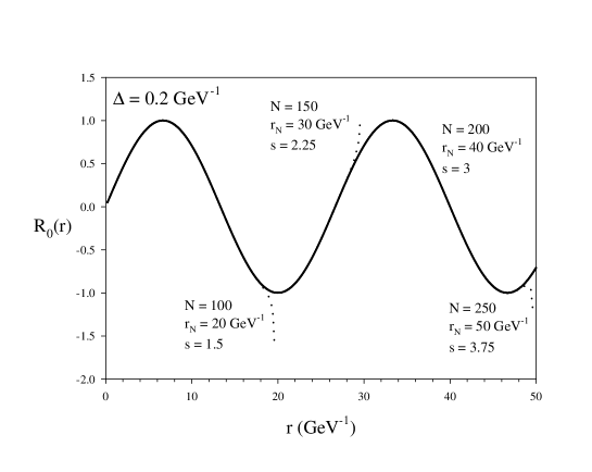
Figure 1: Regularized radial part $R_{0}(r)$ of computed solutions (dotted lines) and the exact solution (solid line) for the semi-relativistic free equation with a given relative kinetic energy and a zero angular momentum. The computed solutions are given for the same spacing, but for different values of $r_{N}$. The value of the parameter $s=N\Delta k/\pi$ is also presented. The energy is chosen in order that $s=3$ for $r_{N}=40$ GeV^-1. All computed wave functions are normalized to match the exact solution.

As noted above, solutions of the non-relativistic and semi-relativistic free Eq. (7) can be expressed in terms of spherical Bessel functions. It can be easily shown that the vector $\{r_{i}\,j_{0}(kr_{i});i=1,\,\ldots,\,N-2\}$, up to a normalization constant, is a solution of the system (20) for $l=0$ if $k=\frac{\pi}{N\Delta}s$ with $s=1,\,\ldots,\,N-2$. This vector is no longer a solution if $k$ is not a integer multiple of $\frac{\pi}{N\Delta}$. In this case the computed solution matches the solution of the continuous Eq. (7) everywhere, except near the last point $r_{N}$ of the domain of integration. This situation is illustrated with Fig. 1 for the semi-relativistic free equation. The regularized radial part of the computed solution for a given energy is presented for the same value of the spacing, but for different values of $r_{N}$. The relative kinetic energy being fixed, different values of $r_{N}$ correspond to different values for the parameter $s$. We can show on this figure that the computed solutions differ from the exact solution when $s$ is not an integer. The situation is not modified by a change of the energy.

If the angular momentum $l$ is different from zero, then the vector $\{r_{i}\,j_{l}(kr_{i})\}$ is not an exact solution of the system (20) or (21). Nevertheless, a very good approximation of the continuous free solution can be obtained with correct values for the parameters $\Delta$ and $r_{N}$. Again, the computed and the exact solutions can differ strongly near the last point $r_{N}$. It is worth noting that the differences between the computed and the exact solutions are much less large in the non-relativistic case, whatever the value of $l$.

In the free case, the phase shift is expected to be zero. Numerically, the phase shift can be determined by using two points of the computed solution. If these points are chosen in the region near $r_{N}$, the phase shift found can be different from zero. On the contrary, when the two points are taken far from $r_{N}$, the phase shift value vanishes.

III.2 Gaussian potential

We have tested our method with different finite range potentials in the case of symmetric or asymmetric systems. In this section, we shall only present some results obtained with a Gaussian potential

$$V(r)=-V_{0}\,e^{-r^{2}/a^{2}},$$ (22)

for two identical particles $m_{1}=m_{2}=m$.

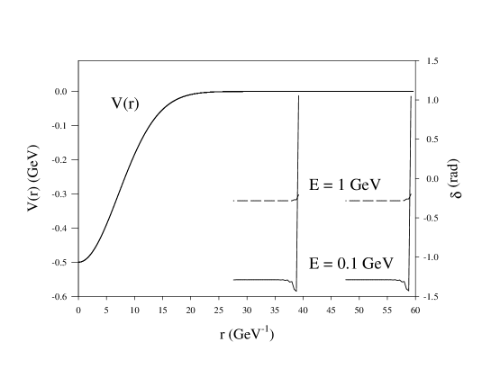
Figure 2: Phase shifts $\delta$ in radians for two identical semi-relativistic particles with $m=1$ GeV, interacting via a Gaussian potential with $V_{0}=0.5$ GeV and $a=10$ GeV^-1. The phase shifts are plotted as a function of $r_{p}$ (see Sec. III.2) for two values of the relative energy and for two values of $r_{N}$. The potential as a function of $r$ is also indicated.

In the free case, the computed solution can differ strongly from the real solution near the last point $r_{N}$. This is also the case when a potential is turned on. The phase shift can be computed with two values of the numerical solution evaluated at two different points $r_{p}$ and $r_{q}$. If $p$ or $q$ is too close to $N$, then the value of the phase shift can be very bad. Obviously, the two points must be taken in a region where the potential can be neglected with respect to the relative kinetic energy. A good procedure to get reliable phase shift is to compute the wave function with a large value of $r_{N}$. Then, the phase shift can be computed with two adjacent points $r_{p}$ and $r_{p-1}$ as a function of the index $p$. By decreasing the value of $p$ from $N$, the phase shifts will first strongly vary and rapidly reach a stable value, as long as $r_{p}$ is large enough to not fall in a region where the potential cannot be neglected. This situation is illustrated with Fig. 2. On this figure, the phase shift for two identical semi-relativistic particles with $m=1$ GeV is plotted as a function of $r_{p}$ for two values of the relative energy and for two values of $r_{N}$. The Gaussian potential is characterized by $V_{0}=0.5$ GeV and $a=10$ GeV^-1. It is worth noting that the variation of the phase shifts are much larger for the semi-relativistic case than for the non-relativistic case.

Scattering states have been calculated with our method for two non-relativistic particles interacting with a Gaussian potential. In this case, wave functions and phases shifts can also be computed with a great variety of methods. For a large range of relative energy and for angular momentum varying from 0 to 4, we have checked that all approaches give same results. Within our method, a relative accuracy of at least $10^{-4}$ for phase shifts can be obtained with a grid containing 200–400 points. Obviously, the interest of our method is to compute scattering solutions in the semi-relativistic case.

It is shown in the appendix that a spinless Salpeter equation with a particular separable non-local potential can be transformed into a Schrödinger-like non-local equation. In this case, the scattering semi-relativistic equation can be solved directly by the Fourier grid Hamiltonian method, or using the equivalent Schrödinger-like form, by usual techniques. We have verified, for several values of the parameters and for different values of the relative kinetic energy, that all methods give the same results. This yields a direct verification of our approach.

Finally, we give, in Table 1, the phase shifts for two identical particles interacting via a Gaussian potential as a function of the relative kinetic energy. Results have been computed for a non-relativistic and a semi-relativistic kinematics, and for two values of the angular momentum $l$. As expected, phase shifts are similar for low relative energy, and differ when energy increases.

IV Summary

The 3-dimensional Fourier grid Hamiltonian method, used in a previous work to compute bound states brau97a , appears as a convenient method to find the scattering solutions of a spinless Salpeter equation (or a Schrödinger equation). It has the advantage of simplicity since it requires only the evaluation of the potential at some grid points and it generates directly the values of the radial part of the wave function at the same grid points. Moreover, the method can be extended to the cases of non-local interaction or coupled channel equations. Up to our knowledge, this is the first time that the scattering solutions of the spinless Salpeter equation are presented.

Meson-meson scattering has been recently investigated in terms of quark degrees of freedom within the framework of the non-relativistic resonating group method ceul96 . From this work, it appears that the use of a semi-relativistic kinematics is necessary to avoid inconsistencies related to the non-relativistic formalism. We have calculated a semi-relativistic version of the pion-pion scattering equation. This equation is a scattering spinless Salpeter equation. In this framework, the method presented here appears suitable to calculate the corresponding phase shifts ceul98 .

The accuracy of the solutions of the numerical method presented here can easily be controlled since it depends only on two parameters: The number of grid points and the largest value of the radial distance considered to perform the calculation. This distance must be large enough to fall in the region where the potential can be neglected with respect to the asymptotic kinetic energy. Both parameters can be automatically increased until a convergence is reached for phase shifts.

The method involves the use of matrices of order $\left(N\times N\right)$, where $N$ is the number of grid points. Generally, the most time consuming part of the method is the solution of the linear system. This is not a problem for modern computers, even for PC stations. Moreover, several powerful techniques exist and can be used at the best convenience. A demonstration program is available via anonymous FTP on umhsp02.umh.ac.be/pub/ftp_pnt/.

Particular case of the spinless Salpeter equation

The spinless Salpeter equation for two identical particles interacting via a non-local potential can be written

$$2\sqrt{\vec{p}\,^{2}+m^{2}}\,\Psi(\vec{r}\,)=M\,\Psi(\vec{r}\,)-\int d\vec{r}\,^{\prime}\,W(\vec{r},\vec{r}\,^{\prime})\,\Psi(\vec{r}\,^{\prime}).$$ (23)

Acting on both sides with the square-root operator gives

$$4\left(\vec{p}\,^{2}+m^{2}\right)\Psi(\vec{r}\,)=M\left(M\Psi(\vec{r}\,)-\int d\vec{r}\,^{\prime}\,W(\vec{r},\vec{r}\,^{\prime})\,\Psi(\vec{r}\,^{\prime})\right)-2\int d\vec{r}\,^{\prime}\,\sqrt{\vec{p}\,^{2}+m^{2}}\,W(\vec{r},\vec{r}\,^{\prime})\,\Psi(\vec{r}\,^{\prime}).$$ (24)

If the potential has the form $W(\vec{r},\vec{r}\,^{\prime})=V_{0}\,V(r)\,V(r^{\prime})$, and if we perform the integrations on angular variables, we obtain

$$\left(\vec{p}\,^{2}+m^{2}-\frac{M^{2}}{4}\right)R_{0}(r)=-\pi V_{0}\left(M+2\sqrt{\vec{p}\,^{2}+m^{2}}\right)V(r)\int_{0}^{\infty}dr^{\prime}\,r^{\prime 2}\,V(r^{\prime})\,R_{0}(r^{\prime}).$$ (25)

where $R_{0}(r)$ is the radial part of the S-wave function $\Psi(\vec{r}\,)$. It has been shown in Ref. brau97b that

$$\sqrt{\vec{p}\,^{2}+m^{2}}\,e^{-mr}=\frac{4m}{\pi}\,K_{0}(mr),$$ (26)

where $K_{0}(x)$ is a modified Bessel function (grad80, , p. 952). In this case, if we choose $V(r)=\exp(-mr)$, then Eq. (23) reduces to a non-local Schrödinger-like equation

$$\left(\frac{d^{2}}{dr^{2}}-m^{2}+\frac{M^{2}}{4}\right)u_{0}(r)=V_{0}\left(M\pi e^{-mr}+8mK_{0}(mr)\right)r\int_{0}^{\infty}dr^{\prime}\,r^{\prime}\,e^{-mr^{\prime}}\,u_{0}(r^{\prime}),$$ (27)

where $u_{0}(r^{\prime})=r^{\prime}R_{0}(r^{\prime})$.

Table 1: Phase shifts for two identical particles with $m=1$ GeV as a function of the relative kinetic energy $E$. The interaction is a Gaussian potential with $V_{0}=0.1$ GeV and $a=5$ GeV^-1 (see Eq. (22)). Results are given for a non-relativistic (NR) and a semi-relativistic (SR) kinematics, and for two values of the angular momentum $l$.

$l$	$E$ (GeV)	$\delta_{\text{NR}}$ (rad)	$\delta_{\text{SR}}$ (rad)
0	0.001	$-$0.192	$-$0.189
	0.01	$-$0.627	$-$0.619
	0.1	1.363	1.376
	1.	0.447	0.524
	10.	0.156	0.256
1	0.001	$-$0.231	$-$0.226
	0.01	$-$0.931	$-$0.925
	0.1	1.241	1.254
	1.	0.479	0.517
	10.	0.156	0.256

References

- (1) William H. Press, Saul A. Teukolsky, William T. Vetterling, and Brain P. Flannerey, Numerical Recipes in FORTRAN (Cambridge University Press, 1992).
- (2) F. Brau and C. Semay, J. Comput. Phys 139, 127 (1998).
- (3) C. Clay Marston and Gabriel G. Balint-Kurti, J. Chem. Phys. 91, 3571 (1989).
- (4) Gabriel G. Balint-Kurti, Christopher L. Ward and C. Clay Marston, Comput. Phys. Commun. 67, 285 (1991).
- (5) Leonard S. Rodberg and Roy M. Thaler, Introduction to the Quantum Theory of scattering (Academic Press, New York, 1967).
- (6) R. Ceuleneer, C. Semay and B. Silvestre-Brac, J. Phys. G 22, 1395 (1996).
- (7) R. Ceuleneer and C. Semay, “Semi-relativistic RGM calculations of pion-pion scattering”, in preparation.
- (8) F. Brau, Integral equation formulation of the spinless Salpeter equation, Preprint Mons 1997, to appear in J. Math. Phys.
- (9) I.S. Gradshteyn and I.M. Ryzhik, Tables of Integrals, Series, and Products (Academic Press, New York, 1980).