Universality of Regge and vibrational trajectories in a semiclassical model

Abstract

The orbital and radial excitations of light-light mesons are studied in the framework of the dominantly orbital state description. The equation of motion is characterized by a relativistic kinematics supplemented by the usual funnel potential with a mixed scalar and vector confinement. The influence of finite quark masses and potential parameters on Regge and vibrational trajectories is discussed. The case of heavy-light mesons is also presented.

I Introduction

One of the most striking feature of the light-light meson spectra is certainly the existence of the so-called “Regge trajectories”, that is to say the linear dependence of the square mass as a function of the total spin quantum number. One can see in Fig. 1 the remarkable linear trajectories of the $\rho$, $K^{\star}$ and $\phi$ families. It is well known that this behavior can be obtained in potential models by using a confinement potential well adjusted for the kinematics. In non-relativistic descriptions of meson spectra, a $r^{2/3}$ confining potential must be used fabr88 , while in relativistic kinematics the linear Regge trajectories are obtained with a linear confinement luch91 and results also naturally from the relativistic flux tube model of mesons laco89 ; sema95 . It is worth noting that this mass behavior is also expected for heavy-light mesons.

An interesting theoretical approach of light-light and heavy-light mesons is given by the dominantly orbital state (DOS) description goeb90 for which the leading Regge trajectory is a “classical” result while radially excited states can be treated semiclassically. In a recent paper olss97 , this DOS model has been applied to study light-light and heavy-light meson spectra with a confinement potential being a mixture of scalar and vector components. In the case of one or two quarks with vanishing masses, it was shown that linear Regge (orbital) and “vibrational” (radial) trajectories are obtained for an arbitrary scalar-vector mixture but that the ratio of radial to orbital energies is strongly dependent on the mixture.

In this paper, we extend the result of Ref. olss97 for light-light and heavy-light mesons by considering the presence of quarks with finite masses and the introduction of a Coulomb-like interaction and constant potential in addition to the confinement. In the limit of small masses and small strength of the short range potential, or in the limit of large angular momentum, all calculations can be worked out analytically. One could expect that the small quark masses and Coulomb-like potential do not need to be taken into account to study high orbitally excited state. But we show here that such effects are interesting to point out. The square mass formula for light-light mesons composed of two identical quarks as a function of quantum numbers and potential parameters is established and discussed in Sec. II. A comparison of our theoretical predictions with data is performed in Sec. III. Some concluding remarks are given in Sec. IV.

II The model

II.1 basic ideas

The starting point of our model is essentially the same as the one presented by Olsson olss97 . Consequently, we just remind the basic ideas and skip a lot of technical details which can be found in that reference. In all our formulae, we use the natural units $\hbar=c=1$.

We consider a system composed of two spinless particles with the same mass $m$, which are allowed to rotate around their center of mass fixed at the origin, and to vibrate in the radial dimension. The Lagrange coordinates are the interdistance $r$ and the rotation angle $\varphi$, angle between an arbitrary fixed direction and the line joining the two particles. The free relativistic Lagrangian is very easy to write and depends on the Lagrange coordinates and their time derivatives. In order to handle the dynamics between the particles, we introduce phenomenologically an interaction potential which depends on the radial coordinate $r$ only. In fact, there exist two Lorentz structures for this potential: a scalar term $S(r)$ which simply modifies the mass ($m\rightarrow m+S(r)/2$), and a vector term $V(r)$ which is simply subtracted from the Lagrangian. Consequently the starting Lagrangian is given by

$$L(r,\varphi,\dot{r},\dot{\varphi})=-\left(2m+S(r)\right)\sqrt{1-\frac{1}{4}\dot{r}^{2}-\frac{1}{4}\dot{\varphi}^{2}r^{2}}-V(r).$$ (1)

This formula can be applied to particles with spin in a very crude manner by considering spin dependent potential terms. One can see that $L$ is independent of $\varphi$. This means that the angular momentum $J=\frac{\partial L}{\partial\dot{\varphi}}$ is a good quantum number. Taking into account this condition, the Hamiltonian of the system can be written as

$$H(r,p_{r},J)=\sqrt{4p_{r}^{2}+\frac{4J^{2}}{r^{2}}+\left(2m+S(r)\right)^{2}}+V(r).$$ (2)

The idea of the model is to make a classical approximation by considering uniquely the classical circular orbits (lowest energy states with given $J$), defined by $r$=$r_{0}$, and thus $\dot{r}=0$ and $p_{r}$=0. Let us denote

$$M_{0}(J)=H(r=r_{0},p_{r}=0,J).$$ (3)

By using the condition $\frac{\partial L}{\partial r}(r=r_{0})=0$ and performing a number of analytical transformations (see Ref. olss97 ), one finds the fundamental equations (with the conventions $S_{0}=S(r_{0})$, and so on)

$$M_{0}(J)=\frac{r_{0}}{2}\left[V^{\prime}_{0}+2\frac{V_{0}}{r_{0}}+\sqrt{{V^{\prime}_{0}}^{2}+4\frac{(2m+S_{0})}{r_{0}^{2}}\left[(2m+S_{0})+S^{\prime}_{0}r_{0}\right]}\right]$$ (4)

and

$$J=\frac{r_{0}^{2}}{2}\left[\frac{1}{2}V^{\prime}_{0}\left(V^{\prime}_{0}+\sqrt{{V^{\prime}_{0}}^{2}+4\frac{(2m+S_{0})}{r_{0}^{2}}\left[(2m+S_{0})+S^{\prime}_{0}r_{0}\right]}\right)+\frac{(2m+S_{0})S^{\prime}_{0}}{r_{0}}\right]^{1/2}.$$ (5)

Equation (5) (which is in general a transcendental equation) allows to calculate $r_{0}(J)$. Once this value is obtained, it is put into Eq. (4) to get $M_{0}(J)$. Up to now, we are in position to obtain only the ground state energy for a given $J$. In order to get the radial excitations, it is useful to make a harmonic approximation around the previous classical orbits. Here again, the details can be found in Ref. olss97 . The harmonic quantum energy is given by

$$\Omega(J)=2\frac{\left[\left(M_{0}(J)-V_{0}\right)V_{0}^{\prime\prime}+{S^{\prime}_{0}}^{2}+(2m+S_{0})S_{0}^{\prime\prime}+\displaystyle{\frac{12J^{2}}{r_{0}^{4}}}-{V^{\prime}_{0}}^{2}\right]^{1/2}}{M_{0}(J)-V_{0}}.$$ (6)

Then the mass of the system with an orbital excitation $J$ and a radial excitation $n$ (0, 1, …) is given, within this approximation, by

$$M(J,n)=M_{0}(J)+\Omega(J)\left(n+\frac{1}{2}\right).$$ (7)

In this general formulation, one sees that there exists, in principle, a coupling between the orbital and the radial excitations. In relativistic descriptions of two particle systems (for example in the meson sector), it is generally the square of the mass which is considered as the function of the orbital and radial quantum numbers. If one assumes that $\Omega(J)\ll M_{0}(J)$ (see Ref. olss97 ), then one can write

$$M^{2}(J,n)=M_{0}^{2}(J)+M_{0}(J)\Omega(J)(2n+1).$$ (8)

II.2 The meson case

II.2.1 The potential

In the previous subsection, we gave a formalism applicable to any type of potential. Such a study could be undertaken from the numerical point of view, by solving the equations giving $r_{0}$ and reporting the value in the expression of $M_{0}$ and $\Omega$. However there are some drawbacks to proceed that way. First, because of non linearity, there can exist several solutions for Eq. (5) and it may be difficult to discriminate between them. Second, the physical analysis is less obvious when the results originate from a numerical treatment. So, it is highly desirable to study a model for which an analytical solution is available.

In Ref. olss97 , the author studied the spectra of the mesons or, more precisely, the Regge trajectories for a system composed of a quark and an antiquark with $m=0$ interacting via a linear confinement potential that is partly scalar and partly vector. He showed that a linear behavior $M_{0}^{2}(J)\propto J$ automatically emerges.

In this paper, we revisit this study, but in a more general framework. First, we relax the constraint of zero mass and consider the mass of the quarks $m$ as a free parameter. Second, we admit a long range linear confinement supplemented by a short range Coulomb part and constant potential. Indeed quantum chromodynamics tells us that it should be so. The one-gluon exchange process gives rise to a Coulomb term of vector type, while multigluon exchanges are responsible for the linear confinement. Since we ignore the Lorentz structure of the confinement, we suppose, as in Ref. olss97 , that it is partly scalar and partly vector. The importance of each one is reflected through a parameter $f$ whose value is 0 for a pure vector, and 1 for a pure scalar.

Thus, in this paper, we apply the previous formalism, with potentials given by

$$S(r)=f\>a\>r$$ (9)

in which $a$ is the usual string tension, whose value should be around 0.2 GeV², and

$$V(r)=(1-f)\>a\>r\>-\>\frac{\kappa}{r}$$ (10)

in which $\kappa$ is proportional to the strong coupling constant $\alpha_{s}$. A reasonable value of $\kappa$ should be in the range 0.1 to 0.6. We will show below that we are able to obtain an analytical solution for this rather realistic situation.

II.2.2 Scaling properties

In our case, we are faced with a number of parameters, whose origin is very different

• the mass $m$ (in GeV), the string constant $a$ (in $\rm{GeV}^{2}$) and the Coulomb constant $\kappa$ (dimensionless) are dynamical parameters;

• the $f$ parameter (dimensionless) reflects our ignorance about the Lorentz structure of the confinement;

• the quantum numbers $J$ and $n$ of the state.

In what follows, we will be interested by the variation of $M^{2}(m,a,\kappa,f,J,n)$ as a function of quantum numbers $J$ and $n$, and for a given set of physical parameters $m,a,\kappa,f$. $M_{0}$ does not depend on $n$, as well as $\Omega$, so that the $n$ dependence is rather obvious (see Eq. (8)). Let us focus on the dependence on $J$ and on the physical parameters. Actually, it is possible to exploit a scaling law in our equation. One can remark that $\sqrt{a}$ is an energy unit, and $\frac{1}{\sqrt{a}}$ a length unit, so that it is advantageous to work with these natural units. Let us define reduced dimensionless quantities, labeled with an overhead bar, relative to these units. Explicitly, we have

$$\overline{m}=\frac{m}{\sqrt{a}}\>;\>\overline{M}_{0}=\frac{M_{0}}{\sqrt{a}}\>;\>\overline{M}=\frac{M}{\sqrt{a}}\>;\>\overline{\Omega}=\frac{\Omega}{\sqrt{a}}\>;\>\overline{r}_{0}=r_{0}\sqrt{a}.$$ (11)

If we put these values into our fundamental Eq. (5), with application to our particular potentials (9-10), we find, after some manipulations, the equation for $\overline{r}_{0}$

$$f^{2}(2f-1)\,\overline{r}_{0}^{8}+4\overline{m}f(2f-1)\,\overline{r}_{0}^{7}+2\left[2\overline{m}^{2}(2f-1)-\kappa f^{2}(1-f)\right]\,\overline{r}_{0}^{6}-8\kappa\overline{m}f(1-f)\,\overline{r}_{0}^{5}$$

$$-\left[4(1-f)\Big{(}(1-f)J^{2}+2\kappa\overline{m}^{2}\Big{)}+f^{2}\Big{(}\kappa^{2}+8J^{2}\Big{)}\right]\,\overline{r}_{0}^{4}-4\overline{m}f\left(\kappa^{2}+4J^{2}\right)\,\overline{r}_{0}^{3}$$

$$-4\kappa\left[\kappa\overline{m}^{2}+2J^{2}(1-f)\right]\,\overline{r}_{0}^{2}+4J^{2}\left(4J^{2}-\kappa^{2}\right)=0.$$ (12)

Equation (4) giving the value of $M_{0}$ leads in this case to

$$\overline{M}_{0}=\frac{(1-2f)\,\overline{r}_{0}^{4}-2\overline{m}f\,\overline{r}_{0}^{3}+4J^{2}-\kappa^{2}}{\overline{r}_{0}\left((1-f)\,\overline{r}_{0}^{2}+\kappa\right)}.$$ (13)

Similarly, Eq. (6) giving the value of $\Omega$ leads to

$$\overline{\Omega}=$$

$$2\,\left\{\left[(1-f)(2f-1)\,\overline{r}_{0}^{6}+3\kappa(2f-1)\,\overline{r}_{0}^{4}+4\kappa\overline{m}f\,\overline{r}_{0}^{3}+3(1-f)(4J^{2}-\kappa^{2})\,\overline{r}_{0}^{2}+(4J^{2}-\kappa^{2})\kappa\right]\right.$$

$$\left.\left[(1-f)\,\overline{r}_{0}^{2}+\kappa\right]\right\}^{1/2}/\left\{\overline{r}_{0}\,\left[-f^{2}\,\overline{r}_{0}^{4}-2\overline{m}f\,\overline{r}_{0}^{3}+4J^{2}\right]\right\}.$$ (14)

Some comments are in order.

• We see that the use of this scaling law allows to reduce the number of parameters to four ($\overline{m},\kappa,f,J$) in the dimensionless quantities.

• If both $m$=0 and $\kappa$=0, it remains only the powers (0,4,8) in Eq. (II.2.2) so that the equation is always soluble by using $\overline{r}_{0}^{4}$ as a variable; one can see that only one relevant physical solution exists. It should be stressed that this case corresponds to the study of (Ref. olss97 ); we checked that our general formalism applied to that peculiar case gives the solution presented in that reference.

• The complicated equation (5) simplifies in our particular case to a polynomial of eighth order in $\overline{r}_{0}$ (Eq. (II.2.2)). In principle, there could exist 8 solutions, but we must reject non physical complex and real negative values, and the real positive values which lead to negative values for $\overline{M}_{0}$ and $\overline{\Omega}$. Starting from the unique physical solution $\overline{r}_{0}(\overline{m}=0,\kappa=0)$, we can expect, by continuity, that there still remains only one physical solution for small values of $\overline{m}$ and $\kappa$. Although we are not able to prove that the physical solution is always unique, it seems that this is a general property; we remarked that this was always true for a wide range of parameters and for the cases for which an analytical solution can be found (see below).

• The linear term in $\overline{r}_{0}$ is always missing in all expressions.

• The special values $f=0$ (pure vector confinement) and $f=1/2$ (half scalar-half vector) lead for Eq. (II.2.2) to a polynomial of 6th order only. Moreover, in the case $f=0$, the polynomial is of 3th order in $r_{0}^{2}$.

• Odd powers of $\overline{r}_{0}$ disappear in Eq. (II.2.2) when $\overline{m}=0$. By choosing $\overline{r}_{0}^{2}$ as a variable, we are left with a 4th order polynomial.

Although the things look quite nice now, it is possible to simplify further, using another scaling law. As one will see, this new scaling law is very powerful and allows to derive universal conclusions concerning Regge trajectories. Indeed, it is possible to eliminate the $J$ dependence with help of the following changes of variables

$$x=\overline{r}_{0}\>J^{-1/2}\;;\;u=\overline{m}\>J^{-1/2}\;;\;v=\kappa\>J^{-1}.$$ (15)

Using these variables, our polynomial (II.2.2) is rewritten

$$f^{2}(2f-1)\,x^{8}+4uf(2f-1)\,x^{7}+2\left[2u^{2}(2f-1)-vf^{2}(1-f)\right]\,x^{6}-8vuf(1-f)\,x^{5}$$

$$-\left[4(3f^{2}-2f+1)+8(1-f)u^{2}v+f^{2}v^{2}\right]\,x^{4}-4uf(v^{2}+4)\,x^{3}$$

$$-4v\left[vu^{2}+2(1-f)\right]\,x^{2}+4(4-v^{2})=0.$$ (16)

The interest of this equation is that the variable $x$ now depends only on 3 variables $x=x(f,u,v)$. Alternatively, one can put Eq. (13) under the form

$$\overline{M}_{0} = J^{1/2}g(f,u,v),$$

$$g(f,u,v) = \frac{(1-2f)\,x^{4}-2uf\,x^{3}+4-v^{2}}{x\left[(1-f)\,x^{2}+v\right]},$$ (17)

and equation (II.2.2) under the form

$$\overline{\Omega}=2J^{-1/2}h(f,u,v),$$

$$h(f,u,v)=$$

$$\left\{\left[(1-f)(2f-1)\,x^{6}+3v(2f-1)\,x^{4}+4vuf\,x^{3}+3(1-f)(4-v^{2})\,x^{2}+(4-v^{2})v\right]\right.$$

$$\left.\left[(1-f)\,x^{2}+v\right]\right\}^{1/2}/\left\{x\,\left[-f^{2}\,x^{4}-2uf\,x^{3}+4\right]\right\}.$$ (18)

Under these forms, the formalism is the most general and the simplest possible. Except very specific cases that we have studied, it is not possible to get an analytical solution for this general formulation. To proceed further, we need to make some kind of approximations.

II.2.3 Regge and vibrational trajectories

From now on, we are interested only in Regge trajectories which give the behavior of $M^{2}$ in term of $J$ for large value of $J$. It is thus natural to consider the values of $u$ and $v$ defined by Eq. (15) as small quantities and to develop $g$ and $h$ functions, given by Eqs. (II.2.2) and (II.2.2), up to order $J^{-1}$ that is to say keeping constant terms, terms with $u$, terms with $u^{2}$ and terms with $v$. Such a calculation is very painful and we have been helped a lot by the MATHEMATICA software. We skip below all the cumbersome details to retain only the important things. Basically we expand $x$ as

$$x=\alpha(f)+\beta(f)\,u+\gamma(f)\,u^{2}+\delta(f)\,v.$$ (19)

We put this expression into Eq. (II.2.2) up to the given order and identify to zero to get the expressions of $\alpha(f)$, $\beta(f)$, $\gamma(f)$ and $\delta(f)$. Then we report the resulting value of $x$ in $g(f,u,v)$ and $h(f,u,v)$, limited again to the desired order to get $\overline{M}_{0}$ and $\overline{\Omega}$. Lastly we used these quantities in Eq. (7) to obtain $M$. It is important to point out that the expression (8) is valid up to our order (the term in $\Omega^{2}$ is of higher order). At the end of this study, the behavior for large $J$ can be traced back, after reintroducing dimensioned quantities, under the exact form

$${M}^{2}=a\,A(f)\,J+B(f)\,m\,\sqrt{a\,J}+C(f)\,m^{2}+a\,D(f)\kappa+a\ E(f)(2n+1)+O(J^{-1/2}).$$ (20)

The coefficients $A$, $B$, $C$, $D$ and $E$ can be obtained analytically. Another coefficient $R(f)=\frac{2\,E(f)}{A(f)}$ is specially important and will be discussed below. Let us define the auxiliary functions $s(f),t(f),y(f)$ by

$$s(f) = (1-f)^{2}+2f^{2}=1-2f+3f^{2},$$

$$t(f) = \sqrt{s(f)+6f^{2}},$$

$$y(f)^{4} = \frac{8}{s(f)+(1-f)\,t(f)}.$$ (21)

Our coefficients are given by

$$A(f) = \frac{y^{2}}{4}\left[t+3(1-f)\right]^{2},$$

$$B(f) = \frac{y}{f}\left[(1+f)(3f-1)+t\,(1-f)\right],$$

$$C(f) = \frac{1}{f^{2}t}\left[t\,(s+f^{2})+(1-f)(2f-1)\right],$$

$$D(f) = -\left[t+3(1-f)\right],$$

$$E(f) = A(f)\sqrt{\frac{t}{t+1-f}},$$

$$R(f) = 2\sqrt{\frac{t}{t+1-f}}.$$ (22)

We plot the various coefficients in Fig. 2. All these quantities are monotonic functions of $f$ and their ranges from $f=0$ to $f=1$ are given below

• $8\geq A(f)\geq 4$;

• $0\leq B(f)\leq 4\sqrt{2}$;

• $8\geq C(f)\geq 3$;

• $-4\leq D(f)\leq-2\sqrt{2}$;

• $4\sqrt{2}\geq E(f)\geq 4$;

• $\sqrt{2}\leq R(f)\leq 2$.

Equation (20) is the exact expression valid for large $J$; we succeeded in getting an analytical expression in our model. It is very powerful since it is universal and the various dependencies are explicitly seen. One can make the following comments.

• The dominant term for large $J$ is linear, so that we recover pure Regge trajectories. As far as the string tension is consider as a constant, the slope of the Regge trajectories $aA(f)$ is universal in the sense that it is independent of the system (it is also independent on the strong coupling constant). Only the confinement drives the behavior; moreover the slope depends on $f$, the percentage of scalar confinement.

• The slope of the vibrational trajectories $2aE(f)$ presents the same characteristics. Even more important, the ratio of the slopes for radial and orbital trajectories $R(f)$ depends only on $f$. This ratio is greater than 1, as indicated by experimental data.

• The next to dominant term behaves like $\sqrt{J}$ and deforms the straight trajectories for low values of $J$. It must be emphasized that this term is due only to a non zero mass and is independent of the strong coupling constant. Moreover, this term is absent whatever the system if the confinement is purely of vector type, since $B(0)=0$.

• The displacement of the trajectories from the origin has three contributions; one $C(f)m^{2}$ is due to the mass, another $aD(f)\kappa$ is due to the strong coupling constant and the last one $aE(f)$ reflects the zero point motion of the harmonic vibration. The position above or below the origin depends upon the relative importance of each contribution (do not forget that $C$ and $E$ are always $>0$ but that $D$ is always $<$0). The zero point energy of the orbital motion cannot obviously be calculated in our model.

• There is no coupling between orbital and radial motion for large $J$ values (absence of terms $nJ$). This is only a consequence of the Coulomb+linear nature of the quark-antiquark potential. This may not be true for other types of potentials.

II.3 Addition of a constant term

It is well known that, in traditional spectroscopy relying upon Schrödinger or spinless-Salpeter equation, it is necessary to add a constant term to the potential in order to get the absolute values of the spectra. In those models, the effect of this constant is just to shift the absolute spectrum keeping the same relative spectrum. One can raise the question of adding a constant potential in our model. We will see that it is not so difficult to answer this question in our framework.

In principle it is possible to add a constant $C_{\text{V}}$ to the vector potential and a constant $C_{\text{S}}$ to the scalar potential. Let us discuss separately these two cases.

If we add a constant $C_{\text{V}}$ to $V(r)$, this does not affect the functions $V^{\prime}(r)$, $S(r)$, and $S^{\prime}(r)$. From Eq. (5), it is clear that the value $r_{0}$ remains unchanged, and thus all the quantities depending on $r_{0}$ remain unchanged except $V_{0}$ which is change to $V_{0}+C_{\text{V}}$. Consequently, from Eq. (4), $M_{0}$ is changed to $M_{0}+C_{\text{V}}$ and $\Omega$ remains unchanged since it depends only on $M_{0}-V_{0}$ (see Eq. (6)). Then $M$ is changed to $M+C_{\text{V}}$. Squaring this quantity and keeping only the terms to good order, the net effect of $C_{\text{V}}$ is to add supplementary terms to the $B$ and $C$ coefficients.

Let us now add a constant term $C_{\text{S}}$ to $S(r)$; $V(r)$ and all the derivatives are unchanged. Since, in Eq. (5), $J$ depends on $S(r)$, $r_{0}$ does depend on $C_{\text{S}}$. But we see that it is always the value $\left(2m+S(r)\right)$ which appears. If we introduce a new mass $m^{\prime}=m+C_{\text{S}}/2$, we see that the new value of $r_{0}$ is simply $r_{0}(m^{\prime},J)$ instead of $r_{0}(m,J)$. Making this replacement in $M_{0}$ and $\Omega$, we see that we have now $M_{0}(m^{\prime},J)$ and $\Omega(m^{\prime},J)$ instead of the non-primed values. So, the only modification in our formalism is just a change from $m$ to $m^{\prime}$. But in doing so, we must consider the new value of $u$ defined with the modified mass $m^{\prime}$ for applying a limited expansion in term of $J$ ($m^{\prime}/\sqrt{a}$ can be small with respect to 1, while $m$ can be large with respect to $\sqrt{a}$). Assuming that such an expansion is justified, the only effect of $C_{\text{S}}$ is to modify the terms in the $\sqrt{J}$ and the constant contributions.

One can now gather both effects into a single formula. Let us define the dimensionless quantities $\epsilon=1+\frac{C_{\text{S}}}{2m}$ and $\eta=\frac{C_{\text{V}}}{m}$. The only effect of adding the constants $C_{\text{V}}$ and $C_{\text{S}}$ is to change, in the universal equation (20), the $B(f)$ and $C(f)$ coefficients by new ones $B^{\prime}(f,\epsilon,\eta)$ and $C^{\prime}(f,\epsilon,\eta)$ defined by

$$B^{\prime}(f,\epsilon,\eta) = \epsilon\,B(f)+2\eta\,\sqrt{A(f)},$$

$$C^{\prime}(f,\epsilon,\eta) = \epsilon^{2}\,C(f)+\eta^{2}+2\epsilon\,\eta\,\frac{t-(1-f)}{2f}.$$ (23)

In particular, the $A$, $D$ and $E$ coefficients are unchanged, so that the slopes of the orbital and radial trajectories are still unchanged in this more elaborated potential, and appears really as universal quantities depending only on scalar-vector mixture in the confinement.

II.4 Heavy-light mesons

The same formalism can be applied to the case of heavy-light mesons in the limit of infinite heavy quark mass, as mentioned in Ref. olss97 . In light-light mesons considered here, two identical quarks orbit at the same distance $r/2$ from the center of mass. For a heavy-light meson, the light quark orbits around the fixed infinitely massive quark at the distance $r$. To obtain the heavy-light Hamiltonian, one must perform the following replacements in the light-light Hamiltonian (2)

• $\displaystyle{\frac{r}{2}}\rightarrow r$;

• $2m+S(r)\rightarrow m+S(r)$;

• $V(r)\rightarrow V(r)$.

After calculation, one obtains

$${M}^{2}=\frac{a}{2}\,A(f)\,J+\frac{1}{2^{3/2}}\,B(f)\,m\,\sqrt{a\,J}+C(f)\,\frac{m^{2}}{4}+a\,D(f)\kappa+a\ E(f)(2n+1)+O(J^{-1/2}).$$ (24)

III Discussion of the model

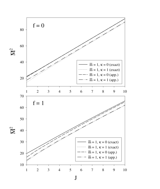
Figure 3: Comparison of the reduced square mass $\overline{M}^{2}$ given by formulae (8,II.2.2-II.2.2) (exact), and the approximate one given by Eq. (20) (app.), as a function of the total angular momentum $J$ for values of $f$, $\overline{m}$ and $\kappa$ equal to 0 and 1, and $C_{\text{S}}=C_{\text{V}}=0$.

Formula (20) gives the meson square mass dependence as a function of parameters. One can ask whether it is possible to extract from this relation values for the parameters by comparing with available data. The value generally considered for the string tension $a$ is around $0.2\pm 0.03$ GeV². Taking $m_{u}\approx m_{d}\approx 0.200$ GeV and $m_{s}\approx 0.450$ GeV, we can see that the parameter $\overline{m}$ runs from 0.5 to 1. The Coulomb strength $\kappa$ is not exactly known, but in potential models a range from 0.1 to 0.6 is currently accepted. So we have to check that formula (20) can be applied for this range of parameters. In Fig. 3, we compare the reduced square mass $\overline{M}^{2}$ calculated exactly by formulae (8,II.2.2-II.2.2) with the one given by Eq. (20), as a function of the total angular momentum $J$ for some values of $f$, $\overline{m}$, $\kappa$ and with $C_{\text{S}}=C_{\text{V}}=0$. One can expect that the quality of the approximation is better for small $\overline{m}$ and $\kappa$ parameters. This is precisely what we get. We present the figure for $\overline{m}=1$, a value already large and, nevertheless, the approximation still works reasonably well. For $f=0$, the approximate value is a pure straight line ($B(0)=0$). The deviation is maximum for large $\kappa$ values, as expected. For $f=1$, there is a small deformation both for the exact solution and the approximate one. Moreover, the curvature is the same in both cases. Note that the concavity of the curve may be inverted by introducing non-vanishing values for $C_{\text{S}}$ and/or $C_{\text{V}}$. For large values of $J$, it is apparent that our approximate expression is always good. For small values of $J$, the deviation is maximum for $\kappa=0$, but we are in a region ($\overline{m}$ large and $J$ small) for which we expect some error. By continuity, other values of $f$ give intermediate situations.

We see that, even in the rather unfavorable case, the approximate expression does not differ so much from the exact results. Consequently, we will base our further discussion on Eq. (20). This last equation can rewritten in the form

$$M^{2}(J,n)={\cal A}\,J+{\cal B}\,\sqrt{J}+{\cal C}+{\cal D}\,n$$ (25)

with ${\cal A}$, ${\cal B}$, ${\cal C}$ and ${\cal D}$ depending on parameters $f$, $a$, $m$, $\kappa$, $C_{\text{S}}$ and $C_{\text{V}}$. Knowing three orbital excitations, for instance $M^{2}(J,n)$, $M^{2}(J+1,n)$ and $M^{2}(J+2,n)$, it is possible to calculate ${\cal A}$ and ${\cal B}$ quantities. Adding a radial excitation, for instance $M^{2}(J,n+1)$, the quantities ${\cal C}$ and ${\cal D}$ can also be calculated. The formulae are given by

$${\cal A} = K_{1,0}(J)\,M^{2}(J+2,n)-K_{2,0}(J)\,M^{2}(J+1,n)+K_{2,1}(J)\,M^{2}(J,n),$$

$${\cal B} = \Delta(J)^{-1}\left[2M^{2}(J+1,n)-M^{2}(J+2,n)-M^{2}(J,n)\right],$$

$${\cal D} = M^{2}(J,n+1)-M^{2}(J,n),$$

$${\cal C} = K_{1,0}(J)\,\sqrt{J(J+1)}\,M^{2}(J+2,n)+K_{2,1}(J)\,\sqrt{(J+1)(J+2)}\,M^{2}(J,n)$$ (26)

$$- K_{2,0}(J)\,\sqrt{J(J+2)}\,M^{2}(J+1,n)-n\left[M^{2}(J^{\prime},n^{\prime}+1)-M^{2}(J^{\prime},n^{\prime})\right],$$

where

$$\Delta(J)=2\sqrt{J+1}-\sqrt{J+2}-\sqrt{J}\quad\text{and}\quad K_{i,j}(J)=\frac{\sqrt{J+i}-\sqrt{J+j}}{\Delta(J)}.$$ (27)

The interest of such formulae is that they are universal in the sense that the quantities ${\cal A}$, ${\cal B}$, ${\cal C}$ and ${\cal D}$ are independent on $J$ and $n$. Given a flavor sector, they could be, in principle, checked for various orbital and radial multiplets. Moreover, the quantities ${\cal A}$ and ${\cal D}$ are even independent on $m$, so that they can be checked independently in several flavor sectors. Finally, the ratio ${\cal D}/{\cal A}$ depends on $f$ only and thus can provide a strong test.

In principle, one could obtain physical quantities from the experimental masses. Starting from ${\cal D}/{\cal A}=R(f)$, one can determine the value of $f$ (see Fig. 2). The quantities $A(f)$, $B(f)$, $C(f)$, $D(f)$ and $E(f)$ can then be calculated. The ${\cal A}$ and ${\cal D}$ quantities can provide us with cross-checked values of the string tension. If $C_{\text{S}}=C_{\text{V}}=0$, the ${\cal B}$ term gives the quark mass $m$; if $C_{\text{S}}\neq 0$ and $C_{\text{V}}\neq 0$, only the quark mass difference in two flavor sectors can be obtained. Calculating parameter $\kappa$ is more involved.

Unfortunately, our model is only valid for high values of $J$, and, for such quantum numbers, a few ground states are known and none radial excitation pdg . Moreover, uncertainties exist about meson masses. Nevertheless, we can try to obtain an estimation of parameter $f$ by considering the mesons of the $\rho$ and $\phi$ families (see Fig. 1).

The meson masses used to perform calculations are center of gravity of meson multiplets whose members are characterized by an internal total spin quantum number equal to one. They are calculated, as well as the corresponding uncertainties, with the procedure given in Ref.brau98 . Using the only three available masses $J$ = 1, 2 and 3 for the $\rho$ family and taking into account the error on these data, we can determine the range possible for the function ${\cal A}=a\,A(f)$. Assuming usual values for the string tension $a$, we can deduce the possible range for $f$. Unfortunately, we obtain no constraint on this parameter since values from 0 to 1 are compatible with data. The same calculation done for the $\phi$ family leads to the conclusion that $f$ must be very close to 0, that is to say that the confinement is only of vector-type. We have remarked that the results are very sensitive to the value of the masses. If other states with higher values of $J$ were known, our conclusion could be changed.

It is also possible to calculate $f$ by considering a meson and its radial excitations (${\cal D}=2a\,E(f)$). This procedure is more questionable since only the first radial excitation of the $J=1$ meson is known in the $\rho$ and $\phi$ families. Nevertheless, if the calculation is performed for the two families, we find that all values for $f$ from 0 to 1 are compatible with the data.

IV Concluding remarks

We have shown that light-light and heavy-light mesons exhibit linear orbital and radial trajectories in the dominantly orbital states (DOS) model. Slopes of both type of trajectories depend only on the string tension and on the vector-scalar mixture in the confinement potential. From our work, it turns out that small finite quark masses do not alter significantly the linearity, specially in the case of dominant vector-type confining potential. As expected, the Coulomb-like potential has no effect on trajectories but its influence on the meson masses has been determined in the approximation of the DOS description. Lastly, we have shown that the ratio of radial to orbital energies depends on the scalar-vector confinement mixture only.

Formula (20) gives the parameter dependence of square mass in the limit of small masses and small strength of the short range potential, or in the limit of large angular momentum. Outside these limits, we have remarked that this formula only differ slightly from exact results in a large range of parameters. This allows to apply our approximation for physical situations and to compare our calculations with experiment.

From data available, it is difficult to determine the value of the parameter $f$, that is to say the scalar-vector mixture in the confinement. Strictly speaking, our results are only semiclassical ones, and experimental radially excited meson masses are only known for small value of total spin. Nevertheless, our calculations favor a dominant vector-type confining interaction.

In our study, we completely neglect the quark spin. Actually, this is not an important drawback. Regge and vibrational trajectories concern only mesons with an assumed internal total spin quantum number equal to one pdg . In usual models the spin-dependent part of the potential is the hyperfine interaction stemming from the one-gluon exchange interaction (and may be from the vector part of the confinement) luch91 . In other models, this spin-dependent part stems from an instanton induced interactions sema95 ; blas90 . In both cases, the contribution of the spin to the meson masses is small or vanishing for mesons with total spin equal to one.

In Sec. II.4, we mentioned a method to study the heavy-light mesons in the limit of an infinitely massive heavy quark. Such a method is used in Ref. olss97 . It could also be interesting to develop the calculations in the more general case of two finite different masses.

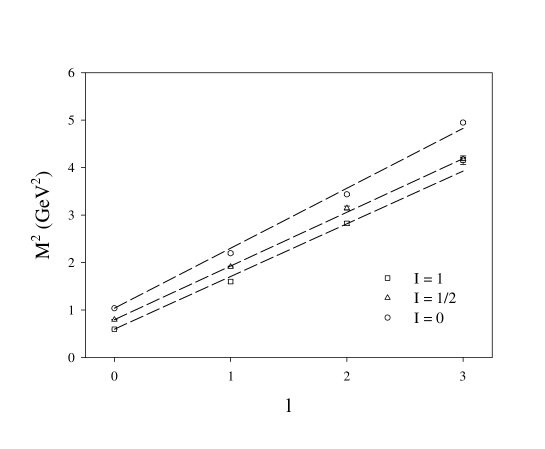
Figure 1: Square mass $M^{2}$ of some light-light mesons as a function of their assumed total orbital angular momentum $l$. The isovector $n\bar{n}$ mesons ($\rho$ family) are indicated by square boxes, strange mesons ($K^{\star}$ family) by triangles and $s\bar{s}$ mesons ($\phi$ family) by circles. The mesons represented are characterized by an internal total spin quantum number equal to one. Excepted for the $l=0$ states, each mass is given by the center of gravity of mesons with the same $l$ but with total spin different (see Sec. III). The remarkable linear dependence is pointed out by straight dashed lines.

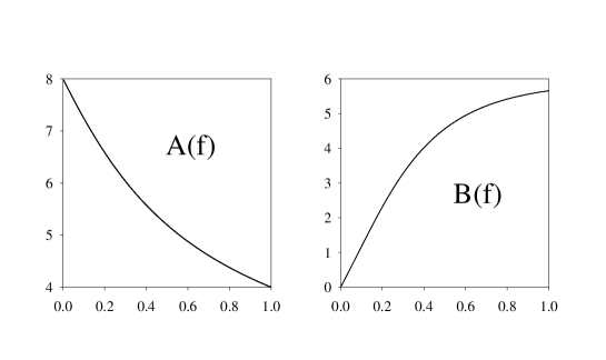
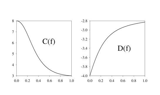
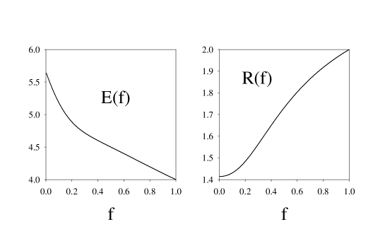
Figure 2: Coefficients giving the square mass (20) as a function of parameter $f$. The ratio $R(f)=2E(f)/A(f)$ is also given.

- (1) M. Fabre de la Ripelle, Phys. Lett. B 205, 97 (1988).
- (2) W. Lucha, F. F. Schöberl and D. Gromes, Phys. Rep. 200, 127 (1991).
- (3) D. LaCourse and M.G. Olsson, Phys. Rev. D 39, 2751 (1989).
- (4) C. Semay and B. Silvestre-Brac, Phys. Rev. D 52, 6553 (1995).
- (5) C. Goebel, D. LaCourse and M. G. Olsson, Phys. Rev. D 41, 2917 (1990).
- (6) M. G. Olsson, Phys. Rev. D 55, 5479 (1997).
- (7) Particle Data Group, R. M. Barnett et al., Phys. Rev. D 54, 1 (1996).
- (8) F. Brau and C. Semay, Phys. Rev. D 58, 034015-1 (1998).
- (9) W. H. Blask et al., Z. Phys. A 337, 327 (1990).