T violation in $B\to K\phi\phi$ decays

Abstract

We present the general form of the decay width angular distributions with T-odd terms in $B\to K\phi\phi$ decays. We concentrate on the T violating effects by considering various possible T-odd momentum correlations. In a generic class of CP violating new physics interactions, we illustrate that the T violating effect could be more than 10%.

One of main goals in $B$ factories is to study CP violation (CPV), which was first discovered in the kaon system CCFT 40 years ago. Recently, Belle BelleCP and Babar BabarCP Collaborations have also confirmed that the CP symmetry is not conserved in the $B$ system. Although the standard model (SM) with three generations could provide a CP violating phase in the Yukawa sector CKM , our knowledge on the origin of CPV is still unclear because it is known that the same CP violating phase cannot explain the observed asymmetry of matter and antimatter. That is, searching a new CP violating source is one of the most important issues in $B$ factories.

As known that the CP-odd quantities which are directly related to the CP violating phases can be defined as the decay-rate difference in a pair of CP conjugate decays. Such kind of the CPV will depend on two phases, one is the weak CP violating phase and the other is the strong CP conserved phase. In addition, one can also define some other useful observables by the momentum correlations. In B physics, T-odd triple-product correlations, denoted by $\vec{p}_{i}\cdot\vec{\varepsilon}^{*}_{1}\times\vec{\varepsilon}^{*}_{2}$, in the two-body $B\to V_{1}V_{2}$ decays, have been studied in Refs. BVV1 ; BVV2 , where $\vec{p}_{i}\ (\vec{\varepsilon}_{i})$ is the three-momentum (polarization) of the vector meson $V_{i}$. The experimental searches for such correlations are in progress at $B$ factories Todd . For three-body B decays, there are many possible types of correlations and the simplest ones are the triple correlations of $\vec{s}\cdot(\vec{p}_{i}\times\vec{p}_{j})$ CG-PRD66 , where $\vec{s}$ is the spin carried by one of outgoing particles and $\vec{p}_{i}$ and $\vec{p}_{j}$ denote any two independent momentum vectors. Clearly, the triple momentum correlations are T-odd observables since they change sign under the time reversal ($T$) transformation of $t\rightarrow-t$. In terms of the CPT invariant theorem, T violation (TV) implies CPV. Therefore, by studying of T-odd observables, it could help us to understand the origin of CPV. We note that these observables of the triple momentum correlations do not require strong phases. In this paper, we study the possibility to observe T violating effects in the three-body decays at B factories.

Recently, Belle Belle-PRL has observed the decay branching ratios (BRs) of $B^{\pm}\to K^{\pm}\phi\phi$ are large, which are $(2.6\pm 0.3)\times 10^{-6}$ with the $\phi\phi$ invariant mass below $2.85$ GeV. By the naive analysis, the decaying mode is dictated by the process $b\to s\bar{s}s$ at the quark level, arising from the one-loop penguin mechanism. In Ref. Hazumi , it has been shown that the direct CP-odd observable associated with a new CP violating phase in the decays could have an excess of $5$ standard deviations with $10^{9}$ B mesons. Since the final states of $B^{\pm}\to K^{\pm}\phi\phi$ involve two vector mesons which provide more degrees of freedom due to spins, many triple momentum correlations can be constructed. It is interesting to investigate the possibility of observing these T-odd observables due to CPV in these decays. We note that Datta and London BVV2 have considered the unique triple momentum correlation with new physics in $B\to\phi K^{*}$ which is also related to the process of $b\to ss\bar{s}$. However, the three-body decays of $B^{\pm}\to K^{\pm}\phi\phi$ contain more T-odd observables in which new physics involved can be different from that in $B\to\phi K^{*}$ and thus our study provides alternative ways to search for T violating effects.

Since the process of $b\to ss\bar{s}$ is dominated by loop effects, for simplicity, the corresponding effective interactions are given by

$$H_{{\rm eff}}={\frac{G_{F}}{\sqrt{2}}}V_{t}\left[a_{1}O_{1}+a_{2}O_{2}+a_{3}O_{3}+a_{4}O_{4}\right]\;,$$ (1)

with the Cabibbo-Kobayashi-Maskawa (CKM) matrix elements $V_{t}=V_{ts}^{*}V_{tb}$ and the operators

$$O_{1} = (\bar{s}b)_{V-A}(\bar{s}s)_{V-A}\;,\;\;\;\;O_{2}=(\bar{s}_{\alpha}b_{\beta})_{V-A}(\bar{s}_{\beta}s_{\alpha})_{V-A}\;,$$

$$O_{3} = (\bar{s}b)_{V-A}(\bar{s}s)_{V+A}\;,\;\;\;\;O_{4}=(\bar{s}_{\alpha}b_{\beta})_{V-A}(\bar{s}_{\beta}s_{\alpha})_{V+A}\;,$$ (2)

where $\alpha$ and $\beta$ are the color indices and the notations $(\bar{q}q^{\prime})_{V\mp A}$ stand for the currents $\bar{q}\gamma_{\mu}(1\mp\gamma_{5})q^{\prime}$. In general, there also exists a right-handed current $(\bar{s}b)_{V+A}$ associated with $b$-quark. However, due to that the corresponding transition matrix element $\langle K|(\bar{s}b)_{V+A}|B\rangle$ involves only the vector current, the contributions from this kind of interactions can be included in Eq. (1) straightforwardly. Moreover, for the Wilson coefficients $a_{i}$ in Eq. (1), the following combinations

$$a^{eff}_{1} = a_{1}+\frac{a_{2}}{N_{c}},\ \ \ a^{eff}_{2}=a_{2}+\frac{a_{1}}{N_{c}},$$

$$a^{eff}_{3} = a_{3}+\frac{a_{4}}{N_{c}},\ \ \ a^{eff}_{4}=a_{4}+\frac{a_{3}}{N_{c}},$$ (3)

with the color factor $N_{c}$ are more useful. It is known that due to the nonperturbative effects, it is difficult to deal with the exclusive nonleptonic decays precisely. In the heavy quark limit, since the particles could be energetic in three-body $B$ decays, accordingly if we could just concentrate on all final state particles in the energetic region, the leading effect will be factorizable parts and those effects from nonfactorizable parts will be subleading. In $B\to K\phi\phi$ decays, the region of the $\phi\phi$ invariant mass measured at Belle is less than the mass of $\eta_{c}$. That is, both $\phi$ mesons are approximately leaving $B$ collinear. Then, in the $B$ rest frame, the whole system looks like a two-body decay. Therefore, outgoing particles are all energetic. Hence, we assume that the factorization parts are dominant. In terms of the factorization assumption, the relevant hadronic transition matrix elements can be parametrized as

$$\langle K(p_{3})|\bar{b}\;\gamma_{\mu}(1-\gamma_{5})s|B(p_{B})\rangle = f_{+}(Q^{2})P_{\mu}+\frac{P\cdot Q}{Q^{2}}Q_{\mu}(f_{0}(Q^{2})-f_{+}(Q^{2})),$$

$$\langle\phi(\epsilon_{1},p_{1})\phi(\epsilon_{2},p_{2})|\bar{s}\;\gamma_{\mu}\;s|0\rangle = \Big{[}\epsilon^{*}_{1}\cdot\epsilon^{*}_{2}A_{1}+{\epsilon^{*}_{1}\cdot Q\,\epsilon^{*}_{2}\cdot Q\over Q^{2}}A_{2}\Big{]}(p_{1}+p_{2})_{\mu}$$ (4)

$$+\Big{[}\epsilon^{*}_{1}\cdot\epsilon^{*}_{2}B_{1}+{\epsilon^{*}_{1}\cdot Q\,\epsilon^{*}_{2}\cdot Q\over Q^{2}}B_{2}\Big{]}(p_{1}-p_{2})_{\mu}$$

$$+C_{1}\epsilon^{*}_{1}\cdot Q\epsilon_{2\mu}+C_{2}\epsilon^{*}_{2}\cdot Q\epsilon_{1\mu},$$

$$\langle\phi(\epsilon_{1},p_{1})\phi(\epsilon_{2},p_{2})|\bar{s}\;\gamma_{\mu}\gamma_{5}\;s|0\rangle = i\varepsilon_{\mu\nu\rho\sigma}\epsilon_{2}^{\nu\ast}p^{\rho}_{1}p^{\sigma}_{2}(\epsilon_{1}^{\ast}\cdot p_{2}){D_{1}\over m^{2}_{\phi}}+i\varepsilon_{\mu\nu\rho\sigma}\epsilon_{1}^{\nu\ast}p^{\rho}_{2}p^{\sigma}_{1}(\epsilon_{2}^{\ast}\cdot p_{1}){D_{2}\over m^{2}_{\phi}}$$ (5)

$$-i\epsilon_{\mu\nu\rho\sigma}\epsilon^{*\nu}_{1}\epsilon^{*\rho}_{2}\Big{(}E(p_{1}+p_{2})^{\sigma}+F(p_{1}-p_{2})^{\sigma}\Big{)},$$

where $\epsilon_{1(2)}$ denote the polarization vectors of the $\phi$ mesons, $P=p_{B}+p_{3}$ and $Q=p_{B}-p_{3}=p_{1}+p_{2}$. The functions $A,B,C,D,E$ and $F$ are the relevant form factors and functions of $Q^{2}$. For simplicity, we neglect to show their explicit $Q^{2}$ dependences. Using the equation of motion, we get

$$\langle V_{1}(\epsilon_{1},p_{1})V_{2}(\epsilon_{2},p_{2})|\bar{s}\;\not{Q}\;s|0\rangle = (m_{s}-m_{s})\langle V_{1}(\epsilon_{1},p_{1})V_{2}(\epsilon_{2},p_{2})|\bar{s}\;s|0\rangle=0\;,$$

$$\langle V_{1}(\epsilon_{1},p_{1})V_{2}(\epsilon_{2},p_{2})|\bar{s}\;(\not{p}_{1}-\not{p}_{2})\gamma_{5}\;s|0\rangle = -iE\varepsilon_{\mu\nu\rho\sigma}(p_{1}-p_{2})^{\mu}\epsilon^{*\nu}_{1}\epsilon^{*\rho}_{2}(p_{1}+p_{2})^{\sigma}=0\;,$$

which imply that $A_{1}=A_{2}=0$, $C_{1}=-C_{2}$, $D_{1}=D_{2}$ and $E=0$. Hence, Eqs. (4) and (5) may be simplified to

$$\langle\phi(\epsilon_{1},p_{1})\phi(\epsilon_{2},p_{2})|\bar{s}\;\gamma_{\mu}\;s|0\rangle = \Big{[}\epsilon^{*}_{1}\cdot\epsilon^{*}_{2}B_{1}+\epsilon^{*}_{1}\cdot Q\,\epsilon^{*}_{2}\cdot Q{B_{2}\over Q^{2}}\Big{]}(p_{1}-p_{2})_{\mu}$$ (6)

$$+C\Big{[}\epsilon^{*}_{1}\cdot Q\epsilon_{2\mu}-\epsilon^{*}_{2}\cdot Q\epsilon_{1\mu}\Big{]}$$

$$\langle\phi(\epsilon_{1},p_{1})\phi(\epsilon_{2},p_{2})|\bar{s}\;\gamma_{\mu}\gamma_{5}\;s|0\rangle = i\frac{D}{m^{2}_{\phi}}\Big{[}(\epsilon_{1}^{\ast}\cdot p_{2})\varepsilon_{\mu\nu\rho\sigma}\epsilon_{2}^{\nu\ast}p^{\rho}_{1}p^{\sigma}_{2}+i(\epsilon_{2}^{\ast}\cdot p_{1})\varepsilon_{\mu\nu\rho\sigma}\epsilon_{1}^{\nu\ast}p^{\rho}_{2}p^{\sigma}_{1}\Big{]}$$ (7)

$$-iF\varepsilon_{\mu\nu\rho\sigma}\epsilon^{*\nu}_{1}\epsilon^{*\rho}_{2}(p_{1}-p_{2})^{\sigma}.$$

In addition, according to the Fierz transformation, the four-Fermi interaction $(V-A)\otimes(V+A)$ can be transformed to $(S-P)\otimes(S+P)$. Hence, the matrix elements associated scalar and pseudoscalar currents can be obtained via equation of motion to be

$$\langle K(p_{3})|\bar{b}\;s|B\rangle = -\frac{P\cdot Q}{m_{b}-m_{s}}f_{0}(Q^{2}),$$

$$\langle\phi(\epsilon_{1},p_{1})\phi(\epsilon_{2},p_{2})|\bar{s}\;s|0\rangle = \frac{Q^{2}-(2m_{\phi})^{2}}{2m_{s}}\epsilon^{*}_{1}\cdot\epsilon^{*}_{2}B_{1}$$

$$+\frac{\epsilon^{*}_{1}\cdot Q\epsilon^{*}_{2}\cdot Q}{2m_{s}}\left(\left(1-\frac{(2m_{\phi})^{2}}{Q^{2}}\right)B_{2}-2C\right),$$

$$\langle\phi(\epsilon_{1},p_{1})\phi(\epsilon_{2},p_{2})|\bar{s}\gamma_{5}s|0\rangle = i\frac{F}{m_{s}}\varepsilon_{\mu\nu\rho\sigma}\epsilon^{*\mu}_{1}\epsilon^{*\nu}_{2}p^{\rho}_{1}p^{\sigma}_{2}.$$ (8)

By combining the results of Eqs. (T violation in $B\to K\phi\phi$ decays), (6), (7) and (8), the transition matrix element for $B\to K\phi\phi$ is expressed by

$${\cal M} = \frac{G_{F}}{\sqrt{2}}V_{ts}V^{*}_{tb}\left\{\left(m_{1}\epsilon^{*}_{1}\cdot\epsilon^{*}_{2}+{m_{2}\over Q^{2}}\epsilon^{*}_{1}\cdot Q\,\epsilon^{*}_{2}\cdot Q\right)p_{B}\cdot(p_{1}-p_{2})+im_{3}\Big{[}{\epsilon^{*}_{2}\cdot Q\over m^{2}_{\phi}}\varepsilon_{\mu\nu\rho\sigma}\epsilon^{*\mu}_{1}p^{\nu}_{2}p^{\rho}_{1}p^{\sigma}_{B}\right.$$ (9)

$$+(1\leftrightarrow 2)\Big{]}+im_{4}\varepsilon_{\mu\nu\rho\sigma}\epsilon^{*\mu}_{1}\epsilon^{*\nu}_{2}(p_{1}-p_{2})^{\rho}p^{\sigma}_{B}+im_{5}\varepsilon_{\mu\nu\rho\sigma}\epsilon^{*\mu}_{1}\epsilon^{*\nu}_{2}p^{\rho}_{1}p^{\sigma}_{2}\Big{\}},$$

where various components are defined as

$$m_{1} = \frac{m_{11}+m_{12}\cos\theta}{p_{B}\cdot(p_{1}-p_{2})}=B_{1}f_{0}\frac{c^{eff}_{3}}{r_{s}}\frac{Q^{2}-(2m_{\phi})^{2}}{p_{B}\cdot(p_{1}-p_{2})}+\frac{4|\vec{p}_{B}||\vec{p}_{1}|}{p_{B}\cdot(p_{1}-p_{2})}B_{1}c^{eff}_{1}f_{+}\cos\theta,$$

$$m_{2} = \frac{m_{21}+m_{22}\cos\theta}{p_{B}\cdot(p_{1}-p_{2})}=Zf_{0}\frac{c^{eff}_{3}}{r_{s}}\frac{Q^{2}}{p_{B}\cdot(p_{1}-p_{2})}+\frac{4|\vec{p}_{B}||\vec{p}_{1}|}{p_{B}\cdot(p_{1}-p_{2})}\frac{Zc^{eff}_{1}f_{+}}{1-\frac{(2m_{\phi})^{2}}{Q^{2}}}\cos\theta,$$

$$m_{3} = -2c^{eff}_{2}f_{+}D,\ \ \ m_{4}=2c^{eff}_{2}f_{+}F,$$

$$m_{5} = 2c^{eff}_{2}\left(\frac{m^{2}_{B}}{Q^{2}}(f_{0}-f_{+})-f_{+}\right)F-2\frac{c^{eff}_{3}}{r_{s}}f_{0}F,$$ (10)

with

$$c^{eff}_{1} = a^{eff}_{3}+a^{eff}_{1}+a^{eff}_{2},\ \ \ c^{eff}_{2}=a^{eff}_{3}-a^{eff}_{1}-a^{eff}_{2},\ \ \ c^{eff}_{3}=a^{eff}_{4},$$

$$Z = \left(1-(2m_{\phi})^{2}/Q^{2}\right)B_{2}-2C\,.$$ (11)

In order to get the spectrum with CP and T violating effects, we choose the relevant coordinates of momenta and polarizations in the rest frame of $Q^{2}$ as

$$Q = (\sqrt{Q^{2}},0,0,0),\ \ E_{B}=\frac{m^{2}_{B}+Q^{2}}{2\sqrt{Q^{2}}},\ \ |\vec{p}_{B}|=|\vec{p}_{K}|=E_{K}=\frac{m^{2}_{B}-Q^{2}}{2\sqrt{Q^{2}}},$$

$$p_{{1(2)}} = (E_{\phi},\pm p_{\phi}\sin\theta,0,\pm p_{\phi}\cos\theta),\ \ E_{\phi}=\frac{\sqrt{Q^{2}}}{2},\ \ p_{\phi}=\sqrt{E^{2}_{\phi}-m^{2}_{\phi}},$$

$$\epsilon_{1(2)L} = \frac{1}{m_{\phi}}(p_{\phi},\pm E_{\phi}\sin\theta,0,\pm E_{\phi}\cos\theta),\ \ \epsilon_{1T}(\pm)=\frac{1}{\sqrt{2}}(0,\cos\theta,\pm i,-\sin\theta),$$

$$\epsilon_{2T}(\pm) = \frac{1}{\sqrt{2}}(0,\cos\theta,\mp i,-\sin\theta),$$ (12)

where $\theta$ stands for the polar angle of the $\phi$ meson. From Eqs. (9) and (12), the differential decay rate for $B\to K\phi\phi$ as a function of $Q^{2}$ is given by

$$\frac{d\Gamma}{dQ^{2}} = {|V_{tb}V_{ts}|^{2}G^{2}_{F}\over 2^{10}\pi^{3}m_{B}}\left(1-\frac{Q^{2}}{m^{2}_{B}}\right)\sqrt{1-\frac{(2m_{\phi})^{2}}{Q^{2}}}\left\{2\left[|m_{11}|^{2}+\frac{2}{3}|m_{12}|^{2}\right]e_{11}\right.$$ (13)

$$+2\left[|m_{21}|^{2}+\frac{2}{3}|m_{22}|^{2}\right]e_{22}+2\left[2Re(m_{11}m^{*}_{21})+\frac{2}{3}Re(m_{12}m^{*}_{22})\right]e_{12}$$

$$\left.+\left(|m_{3}|^{2}e_{33}+|m_{4}|^{2}e_{44}\right)+2Re(m_{3}m^{*}_{4})e_{34}+2|m_{5}|^{2}e_{55}+4Re(m_{4}m^{*}_{5})e_{45}\right\},$$

where

$$e_{11} = 2+\frac{(p_{1}\cdot p_{2})^{2}}{m^{4}_{\phi}},\ \ \ e_{22}=\left(\frac{m^{2}_{\phi}}{Q^{2}}\right)^{2}\left(1-\frac{(p_{1}\cdot p_{2})^{2}}{m^{4}_{\phi}}\right)^{2},$$

$$e_{12} = -\frac{p_{12}}{Q^{2}}\left(1-\frac{p^{2}_{12}}{m_{\phi}^{4}}\right),\ \ \ e_{33}=\frac{4}{3}\frac{8\kappa}{(2m_{\phi})^{2}}\left(1-\frac{p_{12}^{2}}{m^{4}_{\phi}}\right),$$

$$e_{44} = m_{B}^{4}\left(1+\frac{Q^{2}}{m^{2}_{B}}\right)^{2}\left(1-\frac{(2m_{\phi})^{2}}{Q^{2}}\right)-\frac{4}{3}\frac{8\kappa}{(2m_{\phi})^{2}},$$

$$e_{34} = \frac{4}{3}\frac{8\kappa}{(2m_{\phi})^{2}}\left(1-\frac{p_{12}}{m_{\phi}^{2}}\right),\ \ \ e_{55}=2p_{12}^{2}-2m_{\phi}^{4},$$

$$e_{45} = -m^{4}_{B}\left(\frac{m_{\phi}^{2}}{m^{2}_{B}}-\frac{p_{12}}{m^{2}_{B}}\right)\left(1+\frac{Q^{2}}{m^{2}_{B}}\right),$$

$$\kappa = -m^{4}_{B}\frac{Q^{2}}{16}\left(1-\frac{Q^{2}}{m^{2}_{B}}\right)^{2}\left(1-(2m_{\phi})^{2}/Q^{2}\right),$$

$$p_{12} = (Q^{2}-2m_{\phi}^{2})/2$$

and $m_{ij}$ are defined in Eq. (10). We note that to obtain the unpolarized spectrum, we need to sum up the polarizations of $\epsilon_{i}$ with $\sum_{\lambda}\epsilon^{*\mu}_{i}(\lambda)\epsilon^{\nu}_{i}(\lambda)=-g^{\mu\nu}+p_{i}^{\mu}p_{i}^{\nu}/m^{2}_{\phi}$.

As known that the uncertain parts for the calculations of exclusive decays are the hadronic matrix elements, such as the functions of $Q^{2}$, $f_{\pm}$, $A$, $B_{1(2)}$, $C$, $D$ and $F$. Since the form factors for $B\to K$ have been studied well in the literature CG-NPB ; Ali , their $Q^{2}$-dependent functions could be controlled with definite errors. For convenience, according to the results of Ref. CG-NPB , we parametrize the form factors $f_{\pm}(Q^{2})$ to be

$$f_{+}(Q^{2}) = 0.35\left(1-1.246\left(\frac{Q^{2}}{m^{2}_{B}}\right)+0.251\left(\frac{Q^{2}}{m^{2}_{B}}\right)^{2}\right)^{-1},$$

$$f_{-}(Q^{2}) = 0.35\left(1-0.297\left(\frac{Q^{2}}{m^{2}_{B}}\right)-0.40\left(\frac{Q^{2}}{m^{2}_{B}}\right)^{2}\right)^{-1}.$$ (14)

Moreover, since the remaining time-like form factors for $\langle\phi\phi|V_{\mu}(A_{\mu})|0\rangle$ are not studied yet, to get numerical estimations, we assume that they all the time-like form factors have the same magnitude, i.e., $B_{1}\sim B_{2}\sim C\sim D\sim F$. In the following, we use ${\cal F}(Q^{2})$ to denote these form factors. In order to express the form factor as a function of $Q^{2}$, we adopt the following form

$${\cal F}(Q^{2})=e^{i\delta}\left(\frac{a}{Q^{2}}-\frac{b}{Q^{4}}\right)\left[\ln\frac{Q^{2}}{d^{2}}\right]^{-1},$$ (15)

where $\delta$ represents the strong phase. The expansion of $(1/Q^{2})^{n}$ is inspired from Ref. Chua for the $\langle KK^{*}|V_{\mu}(A_{\mu})|0\rangle$ transition and the factor $1/\ln(Q^{2}/d^{2})$ is due to the clue of perturbative QCD BF . Since the BR of $B\to K\phi\phi$ has been measured by Belle, we can use the experimental data to fit the unknown parameters $a$, $b$ and $d$. With the fitted parameters, we can estimate the CP and T violating effects in $B\to K\phi\phi$ decays. Hence, in the SM with B$(B\to K\phi\phi)_{Q<2.85GeV}=2.0\times 10^{-6}$, we set $a=5.$, $b=4.$ and $d=1.0$. The spectrum of the differential decay rate is shown in Fig. 1. Our figure is consistent with that of Ref. FPP in which the authors dressed the problem by considering all possible intermediate states.

Figure 1: The differential decay rates (in units of $10^{-6}$) for $B\to K\phi\phi$ with the invariant mass of $\phi$ meson pairs below $2.85$ GeV.

As emphasized early that to study T violating effects, we have to investigate the polarizations of $\phi$ mesons. Since $\phi$ decays to $KK$ dominantly, we expect that the T violating terms could be related to the angular distribution of $K_{1}$ and $K_{2}$, in which $K_{1}$ denotes the daughter of one of two $\phi$ mesons while $K_{2}$ is that of the other $\phi$ meson. The four-component momenta of $K_{1}$ and $K_{2}$ in their present rest frame are chosen as follows: $p_{1}=(E_{1},E_{1}\sin\theta_{1},0,E_{1}\cos\theta_{1})$ and $p_{2}=(E_{2},E_{2}\sin\theta_{2}\sin\phi,E_{2}\sin\theta_{2}\cos\phi,E_{2}\cos\theta_{2})$ with $E_{1}=E_{2}=m_{\phi}/2$. We note that $E_{1(2)}\approx|\vec{p}_{1(2)}|$ due to the smallness of the kaon mass. Here, $\theta_{1(2)}$ are the polar angles of K-mesons in each $\phi$ meson rest frame. The angle $\phi$ represents the relative angle between two decaying planes, produced by the two $\phi$-meson decays. Hence, the angular distribution associated with T odd terms in $B\to K\phi\phi$ is obtained as

$${d\Gamma_{T-odd}(\theta_{1},\theta_{2},\phi,Q^{2})\over dQ^{2}d\cos\theta_{1}d\cos\theta_{2}d\phi} = \frac{9}{4}{G^{2}_{F}\over 2^{11}\pi^{4}m_{B}}B^{2}(\phi\to KK)\left(1-\frac{Q^{2}}{m^{2}_{B}}\right)\sqrt{1-\frac{(2m_{\phi})^{2}}{Q^{2}}}$$ (16)

$$\times\left\{-\left[\frac{1}{4}\int_{-1}^{1}\rm{Im}(H_{0}(H^{*}_{-}-H^{*}_{+}))d\cos\theta\right]\sin 2\theta_{1}\sin 2\theta_{2}\sin\phi\right.$$

$$\left.+\left[\frac{1}{2}\int_{-1}^{1}\rm{Im}(H_{+}H^{*}_{-})d\cos\theta\right]\sin^{2}\theta_{1}\sin^{2}\theta_{2}\sin 2\phi\right\},$$

$$H_{0} = H(0,0)=p_{B}\cdot(p_{1}-p_{2})\frac{Q^{2}}{(2m_{\phi})^{2}}$$

$$\times\left[2m_{1}\left(1-\frac{2m^{2}_{\phi}}{Q^{2}}\right)+m_{2}\left(1-\frac{(2m_{\phi})^{2}}{Q^{2}}\right)\right],$$

$$H_{\pm} = H(\pm,\pm)=-m_{1}p_{B}\cdot(p_{1}-p_{2})\mp 2m_{4}|\vec{p}_{\phi}|E_{B}\mp m_{5}|\vec{p}_{\phi}|\sqrt{Q^{2}},$$

where $H_{0}$ and $H_{\pm}$ are the longitudinal and transverse polarizations, respectively, and $B(\phi\to KK)$ is the decay branching ratio of $\phi\to KK$. Clearly, the T odd terms are related to not only angles $\theta_{1(2)}$ but also the azimuthal angle $\phi$. We note that the results do not depend on the angle $\theta$, which represents the polar angle of the $\phi$ meson in the $Q^{2}$ rest frame. To study these effects, we define the statistical significances by CG-NPB

$$\bar{\varepsilon}_{i}={\int{\cal O}_{i}\omega_{i}(u_{\theta_{K_{1}}},u_{\theta_{K_{2}}})d\Gamma\over\sqrt{\int d\Gamma\cdot\int{\cal O}_{i}^{2}d\Gamma}}$$ (17)

where $\omega_{i}(u_{\theta_{K_{1}}},u_{\theta_{K_{2}}})=u_{\theta_{K_{1}}}u_{\theta_{K_{2}}}/|u_{\theta_{K_{1}}}\,u_{\theta_{K_{2}}}|$ are sign functions with $u_{\theta_{i}}$ being $\cos\theta_{i}$ or $\sin\theta_{i}$. In the $Q^{2}$ rest frame, the T odd momentum correlations for operators in Eq. (17) are given by

$${\cal O}_{T_{1}} = |\vec{p}_{B}|\frac{\vec{p}_{K_{1}}\cdot(\vec{p}_{B}\times\vec{p}_{K_{2}})}{|\vec{p}_{B}\times\vec{p}_{K_{1}}||\vec{p}_{B}\times\vec{p}_{K_{2}}|}=\sin\phi,$$

$${\cal O}_{T_{2}} = |\vec{p}_{B}|\frac{(\vec{p}_{B}\cdot\vec{p}_{K_{2}}\times\vec{p}_{K_{1}})(\vec{p}_{B}\times\vec{p}_{K_{1}})\cdot(\vec{p}_{K_{2}}\times\vec{p}_{B})}{|\vec{p}_{B}\times\vec{p}_{K_{1}}|^{2}|\vec{p}_{K_{2}}\times\vec{p}_{B}|^{2}}=\frac{1}{2}\sin 2\phi,$$

accompanied with sign functions of $\omega_{T_{1}}(\cos\theta_{K_{1}},\cos\theta_{K_{2}})$ and $\omega_{T_{2}}(\sin\theta_{K_{1}},\sin\theta_{K_{2}})$, respectively.

Although Eq. (16) could indicate the T violating effects, since the definition in Eq. (17) does not represent the real time reversal operator in which the initial state will be reversed to be the final state, the appearance of strong phases also contributes to Eq. (16). That is, $d\Gamma_{T-odd}\propto\sin(\theta_{W}+\theta_{s})$ where $\theta_{W}$ and $\theta_{S}$ are the weak CP and strong phases, respectively. In order to avoid the ambiguity for the nonvanished weak CP and strong phases, we propose to include the corresponding CP-conjugate mode and define the new quantities as

$$\bar{\varepsilon}_{i}(B)+\bar{\varepsilon}_{i}(\bar{B}) \propto \sin(\theta_{W}+\theta_{s})+\sin(-\theta_{W}+\theta_{s})=2\cos\theta_{W}\sin\theta_{s},$$ (18)

$$\bar{\varepsilon}_{i}(B)-\bar{\varepsilon}_{i}(\bar{B}) \propto \sin(\theta_{W}+\theta_{s})-\sin(-\theta_{W}+\theta_{s})=2\sin\theta_{W}\cos\theta_{s}.$$ (19)

Evidently, if a nonvanished value of Eq. (18) is observed , it will indicate the non-negligible relative strong phase between time-like form factors. On the other hand, if nonvanished value of Eq. (19) is measured, it will imply the existence of new physical CP violating phase. Since our purpose is to probe the new CP phases, we concentrate our discussions on the definition of Eq. (19). The problem, whether the strong phases play important contributions, is referred to the experiments.

To illustrate the possibility of observing T violation at $B$ factories, instead of discussing a specific model, we consider a generic class of CP violating new physics interactions with $c^{eff}_{k}=c^{SM}_{k}+e^{i\theta_{k}}|c^{NP}_{k}|$, where $(c^{SM}_{1},\,c^{SM}_{2},\,c^{SM}_{3})=(-0.043,0.033,-0.053)$ are the values in the SM while $\theta_{k}$ and $c^{NP}_{k}$ are related to new physics. For simplicity, we take all $\theta_{k}=\pi/2$. In Fig. 2, we present the significances of T violation for some different values of $|c^{NP}_{i}|$. The solid, dashed, dotted, dash-dotted lines stand for $(c^{NP}_{1},\,c^{NP}_{2},\,c^{NP}_{3})=(-0.02,-0.04,-0.03)$, $(-0.01,-0.05,-0.03)$, $(-0.06,-0.02,-0.04)$, and $(0,-0.06,-0.03)$, with the corresponding BRs in turn being $2.53,\,2.63,\,2.78$, and $2.77\times 10^{-6}$, respectively. According to the results of Fig. 2, we clearly see that the contribution of ${\cal O}_{T_{2}}$ is much larger than that of ${\cal O}_{T_{1}}$; and the effect could be more than 10%. We note that to measure this T violating effect at $2\sigma$ level, at least $1.5\times 10^{8}$ B decays are required if we use B$(B\to K\phi\phi)=2.6\times 10^{-6}$. Certainly, it could be detectable at the $B$ factories.

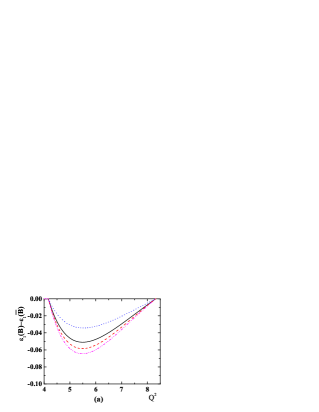
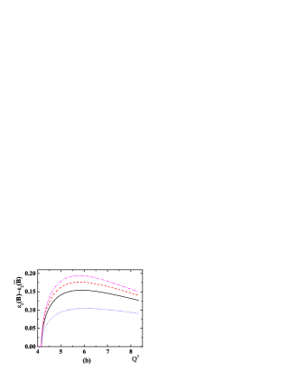
Figure 2: The significances of T violation for (a) ${\cal O}_{T_{1}}$ and (b) ${\cal O}_{T_{2}}$ with respect to the invariant mass of $\phi$ meson pairs below $2.85$ GeV. The sold, dashed, dotted, dash-dotted line stand for the different vales of $c^{NP}_{i}$. The detailed description is in the text.

Finally, we give some remarks on the resonant contributions to the decays. It was pointed out in Ref. FPP that the main resonant contributions to the decay BR are from $\eta_{c}(2980)$ and the changes are around $\pm 10\%$, depending on the constructive or destructive interference. Although the width of $\eta_{c}$ is as small as $17.3$ MeV, since the spectrum for the decaying rate is increasing at $Q^{2}\sim 2.85$, as shown in Fig. 1, the influence on the decay BR may not be neglected. However, the T-odd effects as shown in Fig. 2 are decreasing when $Q^{2}$ is approaching to the upper limits of data. In order to avoid the contributions from resonant effects, we can search the T-odd effects in the region which is far away from the resonant state $\eta_{c}$. In our study, the best searching region of $Q^{2}$ is between $5$ and $7$ GeV².

In summary, by the factorization assumption, we have studied the T-odd observables in $B\to K\phi\phi$ decays. Despite the hadronic uncertainties, we find that the T violating effect for ${\cal O}_{T_{2}}$ could reach $10\%$. Although the resultant depends on the strong phases, as shown in Eq. (18) and (19), we can define the proper T-odd observables associated with the CP conjugate modes so that the experiments can tell us how much the effects are from the CP conserved strong phases.

Acknowledgments

This work is supported in part by the National Science Council of R.O.C. under Grant #s: NSC-91-2112-M-001-053, NSC-93-2112-M-006-010 and NSC-93-2112-M-007-014.

References

(1) J.H. Christenson, J.W. Cronin, V.L. Fitch and R. Turly,
Phys. Rev. Lett. 13, 138 (1964).
(2)Belle Collaboration, K. Abe et al.,
Phys. Rev. D66, 071102 (2002).
(3)Babar Collaboration, B. Aubert et al.,
Phys. Rev. Lett.89, 201802 (2002).
(4) N. Cabibbo, Phys. Rev. Lett. 10, 531 (1963); M.
Kobayashi and T. Maskawa, Prog. Theor. Phys. 49, 652 (1973).
(5) G. Valencia, Phys. Rev. D39, 3339 (1989).
(6)
A. Datta and D. London, Int. J. Mod. Phys. A19, 2505 (2004).
(7) BABAR Collaboration, J.G. Smith, hep-ex/0406063, contribution to Moriond QCD proceedings;
BELLE Collaboration, K. Abe et al., hep-ex/0408141.