A mass formula for light mesons from a potential model

Abstract

The quark dynamics inside light mesons, except pseudoscalar ones, can be quite well described by a spinless Salpeter equation supplemented by a Cornell interaction (possibly partly vector, partly scalar). A mass formula for these mesons can then be obtained by computing analytical approximations of the eigenvalues of the equation. We show that such a formula can be derived by combining the results of two methods: the dominantly orbital state description and the Bohr-Sommerfeld quantization approach. The predictions of the mass formula are compared with accurate solutions of the spinless Salpeter equation computed with a Lagrange-mesh calculation method.

I Introduction

Semirelativistic potential models have been proved extremely successful for the description of light mesons (mesons containing $u$, $d$, or $s$ quarks). The main characteristics of the spectra of these mesons, except pseudoscalar ones, can be obtained with a spinless Salpeter equation supplemented with the Cornell interaction (a Coulomb-like potential plus a linear confinement) fulc94 ; brau98 .

Numerous techniques have been developed in order to solve numerically with a great accuracy the semirelativistic equation. Nevertheless, it is always interesting to work with analytical results. Several attempts to obtain some mass formulae for hadrons were already performed. Some approaches rely on fundamental QCD properties sing82 ; morp90 , but they are limited to the study of ground states of hadrons. In other works, the hadron masses are given as a function of some quantum numbers. They are based, for instance, on shifted large-$N$ expansion ($N$ is the number of spatial dimensions) of the Schrödinger equation pagn86 , a spectrum generating algebra iach91 , or a completely phenomenological point of view sema95 . We will adopt here a different point of view by assuming that a semirelativistic potential model allows a good description of the main features of meson spectra.

Recently, a new method to tackle this problem was developed: the dominantly orbital state (DOS) description, in which the orbitally excited states are obtained as a classical result while the radially excited states are treated semiclassically goeb90 ; olss97 ; silv98 ; brau00a . A second method is the Bohr-Sommerfeld quantization (BSQ) approach, with which precise information can be obtained on the asymptotical behaviors of observables as a function of the quantum numbers brau00b . We show here that a quite well accurate mass formula for light mesons, as a function of quantum numbers and parameters of a QCD inspired potential, can be obtained by combining the results of these two approaches. The idea is to calculate analytical approximate solutions of the equation assumed to govern the quark dynamics inside a meson. There is yet some uncertainties about the Lorentz structure of the interquark interaction. In this work, we will assume that the confinement potential is partly scalar and partly vector. A related work using a WKB approach was performed in Ref. cea82 , but the Coulomb-like potential and the Lorentz structure of the confinement interaction were not taken into account.

In order to test the validity of the mass formula, we compare its predictions with accurate numerical solutions of the spinless Salpeter equation. These last ones are computed with a Lagrange-mesh calculation method sema01 . This technique is here modified in order to handle semirelativistic equations with mixed scalar-vector potentials.

In Sec. II, the model Hamiltonian is presented with the two methods previously developed to compute some analytical solutions. The mass formula is established in the case of symmetric and asymmetric mesons, with our without a constant term in the potential. In Sec. III, the mass formula is compared with accurate numerical solutions of the spinless Salpeter equation. Some concluding remarks are given in Sec. IV.

II The model

II.1 Model Hamiltonian

Within the framework of a semirelativistic potential model, it is possible to describe the main characteristics of the spectra of light mesons fulc94 ; brau98 . If the spinless Salpeter equation is chosen, instead of the Schrödinger equation, the quark-antiquark Hamiltonian is given by (we use the natural units $\hbar=c=1$)

$$H=\sqrt{\vec{p\,}^{2}+\left(m_{1}+\alpha_{1}S(r)\right)^{2}}+\sqrt{\vec{p\,}^{2}+\left(m_{2}+\alpha_{2}S(r)\right)^{2}}+V(r),$$ (1)

where $V(r)$ and $S(r)$ are respectively the vector and scalar interactions goeb90 , and where $\vec{p}$ is the relative momentum between the quark and the antiquark. The vector $\vec{p}$ is the conjugate variable of the inter-distance $\vec{r}$. As usual, we assume that the isospin symmetry is not broken, that is to say that the $u$ and $d$ quarks have the same mass (in the following, these two quarks will be named by the symbol $n$). The parameters $\alpha_{1}$ and $\alpha_{2}$ indicate how the scalar potential $S(r)$ is shared among the two masses $m_{1}$ and $m_{2}$. A natural choice, used in this work, is to take

$$\alpha_{1}=\frac{m_{2}}{m_{1}+m_{2}}\quad\text{and}\quad\alpha_{2}=\frac{m_{1}}{m_{1}+m_{2}}.$$ (2)

It is generally admitted that the short range part of the interquark potential is dominated by the one-gluon exchange process, which gives rise to a Coulomb term of vector type. The long range part is dominated by a confinement that lattice calculations predict linear in the interquark distance. As its Lorentz structure is not precisely known, we suppose here that the confinement is partly scalar and partly vector, as in Ref. olss97 . The importance of each one is reflected through a parameter $f$ whose value is 0 for a pure vector, and 1 for a pure scalar. Consequently, the potentials considered here are given by

$$S(r)=f\,a\,r$$ (3)

in which $a$ is the usual string tension, whose value should be around 0.2 GeV², and

$$V(r)=(1-f)\,a\,r-\frac{\kappa}{r}$$ (4)

in which $\kappa$ is proportional to the strong coupling constant $\alpha_{s}$. A reasonable value of $\kappa$ should be in the range 0.1 to 0.6.

It is worth noting that it is not possible to describe the pseudoscalar mesons with a so simple potential. Spin contributions are very large in this sector as well as flavor mixing effects. An interaction stemming from instanton effects, which is not considered here, could explain the properties of these mesons brau98 ; blas90 . Consequently, the pseudoscalar mesons cannot be described by our model.

II.2 Semi-classical method

Approximate analytical solutions of Hamiltonian (1) with potentials (3)-(4) can be obtained within the DOS approach. The idea of the model is to make a classical approximation by considering uniquely the classical circular orbits (lowest energy states with given total orbital angular momentum $J$), defined by $r$ constant, and thus $\dot{r}=0$. The radial excitations, numbered with the quantum number $\nu$, are calculated by making a harmonic approximation around the previous classical orbits. A detailed description of this method is given in Refs. goeb90 ; olss97 ; silv98 ; brau00a . We just recall here the main results. In the case of a symmetric meson, $m_{1}=m_{2}=m$, the square meson mass $M^{2}$ is given by silv98

$$M^{2}=a\,A(f)\,J+B(f)\,m\,\sqrt{a\,J}+C(f)\,m^{2}+a\,D(f)\kappa+a\ E(f)(2\nu+1)+O(J^{-1/2}).$$ (5)

The coefficients $A$, $B$, $C$, $D$, and $E$ are given by

$$A(f) = \frac{y^{2}}{4}\left[t+3(1-f)\right]^{2},$$

$$B(f) = \frac{y}{f}\left[(1+f)(3f-1)+t\,(1-f)\right],$$

$$C(f) = \frac{1}{f^{2}t}\left[t\,(s+f^{2})+(1-f)(2f-1)\right],$$

$$D(f) = -\left[t+3(1-f)\right],$$

$$E(f) = A(f)\sqrt{\frac{t}{t+1-f}},$$ (6)

where the auxiliary functions $s$, $t$, and $y$ are written

$$s(f) = 1-2f+3f^{2},$$

$$t(f) = \sqrt{s(f)+6f^{2}},$$

$$y(f)^{4} = \frac{8}{s(f)+(1-f)\,t(f)}.$$ (7)

The coefficients $A$, $B$, $C$, $D$, and $E$ are monotonic functions of $f$ and their ranges from $f=0$ to $f=1$ are $8\geq A(f)\geq 4$, $0\leq B(f)\leq 4\sqrt{2}$, $8\geq C(f)\geq 3$, $-4\leq D(f)\leq-2\sqrt{2}$, and $4\sqrt{2}\geq E(f)\geq 4$. Expression (5) is valid for small values of $m/\sqrt{a}$ and $\kappa$, and/or large values of $J$.

As this method relies basically on a classical approximation, it is not possible to calculate the zero point energy of the orbital motion. Thus, a mass formula cannot be obtained. Moreover, the dependence of the energy as a function of the radial quantum number $\nu$ is calculated by making a harmonic approximation around classical orbits with high values of $J$. We cannot expect a good $\nu$ behavior for small values of the angular momentum. A more serious flaw is that the method predicts a linear dependence of $M^{2}$ as a function of $\nu$ whatever the form of the potential. So, we cannot be sure that the $\nu$ dependence found is the more appropriate. A way to correct these drawbacks is to complete the previous analysis by a BSQ method.

II.3 BSQ method

The basic quantities in the BSQ approach tomo62 are the action variables,

$$J_{s}=\oint p_{s}\,dq_{s},$$ (8)

where $s$ labels the degrees of freedom of the system, and where $q_{s}$ and $p_{s}$ are the coordinates and conjugate momenta; the integral is performed over one cycle of the motion. The action variables are quantized according to the prescription

$$J_{s}=\nu_{s}+1/2,$$ (9)

where $\nu_{s}$ ($\geq 0$) is an integer quantum number. This corresponds to a WKB expansion limited to the first order in $h$ (see for instance dunh32 ; bend77 ; robn97a ; robn97b ).

The calculations for the angular momentum $J$, in the limit of great values for this quantum number, give simply the same $J$ dependence for $M^{2}$ as in expression (5), but with $J$ replaced by $J+1/2$. The calculations for the radial motion are more involved. A detailed description of the procedure is given in Ref. brau00b where the case of the Hamiltonian (1) is studied for $m_{1}=m_{2}$ and $f=0$. We use here the same technique and we expand all expressions in powers of the meson mass $M$. Assuming that $M^{2}/a$ is large and $J$ finite, and keeping only terms in $M^{2}$, $M$, and $1/M$, the integral (8) with Hamiltonian (1) can be written, after tedious calculations,

$$\pi(2\nu+1)=\frac{\sqrt{Y}Z}{2a(1-2f)}-\frac{X^{2}}{2a(1-2f)^{3/2}}\ln\left(\frac{Z+\sqrt{(1-2f)Y}}{X}\right),$$ (10)

with $\nu$ the radial quantum number, and with

$$X = Mf+2m(1-f),$$

$$Y = M^{2}-4m^{2}+2a\kappa(1-f)+4am\kappa f/M,$$

$$Z = M(1-f)+2mf+a\kappa(1-2f)/M.$$ (11)

The expression above is valid only for $f\leq 1/2$. A similar equation exists for $f\geq 1/2$. It is now necessary to extract $M^{2}$ as a function of $\nu$ in order to obtain an analytical result usable in a mass formula. If we assume that quantities $m/\sqrt{a}$ and $\kappa$ are small, we can expand Eq. (10) in powers of these small parameters. The first order gives ($m/\sqrt{a}=\kappa=0$)

$$M^{2}\approx aE^{\prime}(f)(2\nu+1)\quad\text{for}\quad\nu\gg 1,$$ (12)

with

$$E^{\prime}(f)=2\pi\frac{1-2f}{1-f-f^{2}H(f)}\quad\text{with}\quad H(f)=\left\{\begin{array}[]{lll}\frac{1}{\sqrt{1-2f}}\ln\left(\frac{1+\sqrt{1-2f}}{1-\sqrt{1-2f}}\right)&\text{for}&f\leq 1/2,\\ \frac{1}{\sqrt{2f-1}}\arccos\left(\frac{1-f}{f}\right)&\text{for}&f\geq 1/2.\end{array}\right.$$ (13)

We have $E^{\prime}(0)=2\pi$, $E^{\prime}(1/2)=3\pi/2$, and $E^{\prime}(1)=4$. This is in agreement with results obtained in Ref. brau00b for the case $f=0$.

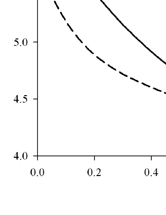
Figure 1: Coefficients $E(f)$ and $E^{\prime}(f)$.

The $\nu$ square mass dependence obtained with this method is very similar to the one obtained with the DOS approach. But, the coefficients $E(f)$ and $E^{\prime}(f)$ are different, as it is shown on Fig. 1. The approximations used to calculate these coefficients are also very different: $E(f)$ is expected to give good results when $J\gg\nu$, while $E^{\prime}(f)$ is expected to give good results when $\nu\gg J$.

By expanding the right hand side of Eq. (10) in powers of $m/\sqrt{a}$ and $\kappa$, we obtain, at the second order,

$$\pi(2\nu+1)\approx\frac{M^{2}\pi}{aE^{\prime}(f)}+\frac{Mmf}{a(1-2f)^{3/2}}\left(\Delta(f)-\frac{\Delta(f)f}{\Delta(f)-f}+2(f-1)\ln\left[\frac{\Delta(f)}{f}-1\right]\right)+\kappa.$$ (14)

where $\Delta(f)=1+\sqrt{1-2f}$ (note that this expression is well defined for $f$ in the range [0,1]). We give these expressions for the sake of completeness. Nevertheless, as we can see below, the first order term is sufficient for our purpose.

II.4 Mass formula

Using results from the DOS approach and the BSQ method, we can write a square mass formula for light mesons composed of two identical quarks with a mass $m$ as a function of the quantum numbers $J$ and $\nu$, and the parameters of the potentials $a$, $\kappa$, and $f$

$${M}^{2}=a\,A(f)\,(J+1/2)+B(f)\,m\,\sqrt{a\,(J+1/2)}+C(f)\,m^{2}+a\,D(f)\kappa+a\ E^{(^{\prime})}(f)(2\nu+1).$$ (15)

The coefficients $A$, $B$, $C$, $D$, and $E$ are given by relations (II.2)-(II.2), and the coefficient $E^{\prime}$ is given by relation (13).

Actually, this formula is an approximate expression for eigenvalues of the Hamiltonian (1). In principle, it is only valid for large values of $J$ and/or large values of $\nu$. The coefficient $E(f)$ will be preferred when $J\gg\nu$, while the coefficient $E^{\prime}(f)$ will be chosen when $\nu\gg J$. One can ask if the Eq. (15) can give good meson mass estimations for realistic values of the potential parameters and for small values of the quantum numbers. In order to answer this question, and then to test the relevance of such a formula, it is necessary to compare the predictions of the formula with accurate numerical solutions of Hamiltonian (1). This is the purpose of Sec. III.

II.5 Addition of a constant term

It is well known that it is necessary to take into account the contribution of a constant term in potential models in order to get the correct absolute values of the meson masses. In principle it is possible to add a constant $\Lambda_{V}$ to the vector potential and a constant $\Lambda_{S}$ to the scalar potential. As in the case of the confinement potential, we can define a parameter $g$ whose value is 0 for a pure vector constant, and 1 for a pure scalar constant

$$\Lambda_{V}=(1-g)\Lambda\quad\text{and}\quad\Lambda_{S}=g\Lambda.$$ (16)

A detailed discussion of the contributions of these two constants is given in Ref. silv98 . But it is very easy to see that the introduction a scalar constant is equivalent to a redefinition of the quark masses, while a vector constant simply shifts all meson masses. Finally, if $M(m,\Lambda)$ is the mass of a meson containing two identical quarks interacting with the potential (3)-(4) supplemented by a constant $\Lambda$ given by Eq. (16), then we have

$$M(m,\Lambda)=M(m+g\Lambda/2,0)+(1-g)\Lambda.$$ (17)

Let us note that, as $\Lambda$ is always negative in realistic potential models, we have $m+g\Lambda/2\leq m$. Then, the formula (17) gives a better approximation than without a constant, since it relies on an expansion for a small mass parameter.

II.6 Asymmetric mesons

The study of mesons containing two different quarks in the framework of the DOS approach has been performed in Ref. brau00a . A formula for the square mass very similar to the expression (5) has been found but with coefficients given only numerically. As these coefficients cannot be determined analytically, they are useless for a mass formula.

Fortunately, one can verify experimentally that the mass of a $n\bar{s}$ meson is in very good approximation the arithmetic mean between the masses of the corresponding $n\bar{n}$ and $s\bar{s}$ mesons. Then, since the mass formula (15) reproduces reasonably well the mass of a symmetric meson, as we will see in Sec. III, it is natural to try the following prescription

$$M(m_{1},m_{2})=\frac{M(m_{1},m_{1})+M(m_{2},m_{2})}{2},$$ (18)

where $M(m,m)$ is the mass of a symmetric meson given by Eq. (15), and $M(m_{1},m_{2})$ the mass of an asymmetric meson containing two quarks with masses $m_{1}$ and $m_{2}$. Equation (18) is then purely phenomenological.

It is worth noting that the scalar potential and the scalar constant are equally shared between the two quarks in a symmetric meson. This is not the case for an asymmetric meson. The relation (18) does not take into account this situation. We will verify below that this does not spoil the quality of the mass formula for asymmetric mesons.

III Discussion of the model

In order to test the relevance of the square mass formula given by Eqs. (15), (17), and (18), we have compared its predictions with the exact eigenvalues of Hamiltonian (1). They are obtained with a great accuracy by using a Lagrange-mesh calculation method for semirelativistic equations sema01 . This method is described in the appendix, with the modification which must be made in order to handle the spinless Salpeter equation with mixed scalar-vector potentials.

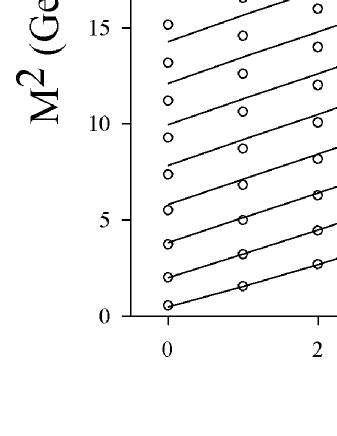
Figure 2: Square masses $M^{2}$ of $n\bar{n}$ mesons as a function of $\nu$ and $J$ quantum numbers, with parameters of Ref. fulc94 , and for $g=0$ and $f=0$. Solid lines join exact solutions of the spinless Salpeter equation. Approximate results from Eq. (15) with the coefficient $E(f)$ are indicated by circles.

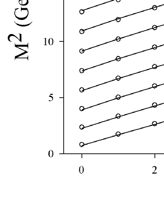
Figure 5: Square masses $M^{2}$ of $n\bar{s}$ mesons as a function of $\nu$ and $J$ quantum numbers, with parameters of Ref. fulc94 , and for $g=0.5$ and $f=0.5$. Solid lines join exact solutions of the spinless Salpeter equation. Approximate results from Eq. (18) with the coefficient $E^{\prime}(f)$ are indicated by circles.

Realistic values for the quark masses and parameters of the potential are taken from a simple semirelativistic model described in Ref. fulc94 : $m_{n}=0.150$ GeV, $m_{s}=0.364$ GeV, $a=0.203$ GeV², and $\kappa=0.437$ ($m_{n}/\sqrt{a}=0.33$ and $m_{s}/\sqrt{a}=0.81$). In this paper, several constants are used, depending on the quark contents of the meson. Here we have just used the constant for $n\bar{n}$ meson, $\Lambda=-0.599$ GeV. The parameters are chosen to reproduce the main features of the meson spectra with $f=g=0$. As, We have used these parameters in our square mass formula with varying values of $f$ and $g$, we cannot obtain good spectra for all values of these two quantities. But the purpose of this work is simply to show the relevance of the mass formula. In Fig. 2 to Fig. 5, we compare the exact eigenvalues of Hamiltonian (1) with the predictions of the mass formula given by Eqs. (15), (17), and (18).

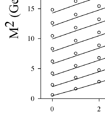
Figure 3: Same as Fig. 2 but for Eq. (15) with the coefficient $E^{\prime}(f)$.

In Fig. 2, the square $n\bar{n}$ meson masses are plotted as a function of $J$ and $\nu$ for parameter values $f=g=0$, the coefficient $E(f)$ being used ($E(f)$ and $E^{\prime}(f)$ are the most different for $f=0$). We can see that for small values of $\nu$ or large values of $J$, the exact and approximate results are in good agreement. This situation is expected when the coefficient of the quantum number $\nu$ is obtained with the DOS approach. For instance, for $J=0$, the relative error on square mass increases regularly from 3.3% at $\nu=2$ to 8.3% at $\nu=9$ (there are irregularities between $\nu=0$ and $\nu=2$). In Fig. 3, the same quantities are plotted, but the approximate results are calculated with the coefficient $E^{\prime}(f)$. In this case, for $J=0$, the absolute error on square mass increases regularly from 0.120 GeV at $\nu=0$ to 0.570 GeV at $\nu=9$, but in the same time, the relative error decreases from 24.5% to 3.1%. This is again the expected behavior for a coefficient of the quantum number $\nu$ obtained with the BSQ method. In the sector where the coefficients $E(f)$ and $E^{\prime}(f)$ are different, it is interesting to choose the coefficient of the quantum number $\nu$ following the values of the quantum numbers $J$ and $\nu$. With this constraint, the results of the square mass formula are quite good.

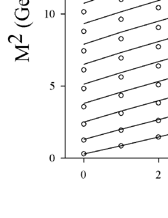
Figure 4: Square masses $M^{2}$ of $n\bar{n}$ mesons as a function of $\nu$ and $J$ quantum numbers, with parameters of Ref. fulc94 , and for $g=0$ and $f=1$. Solid lines join exact solutions of the spinless Salpeter equation. Approximate results from Eq. (15) are indicated by circles ($E^{\prime}(1)=E(1)$).

When $f=1$, the situation is simpler since $E(f)$ and $E^{\prime}(f)$ are identical. In Fig. 4, the square $n\bar{n}$ meson masses are plotted as a function of $J$ and $\nu$ for parameter values $f=1$ and $g=0$. Again the agreement between exact and approximate results is good. The qualities of the mass formula seems to deteriorate with increasing values of $\nu$. Actually, for $J=0$, the absolute error on square mass increases regularly from 0.148 GeV at $\nu=2$ to 0.674 GeV at $\nu=9$, but in the same time, the relative error decreases slowly from 5.9% to 5.5% (there are irregularities between $\nu=0$ and $\nu=2$).

Finally, we have tested the formula (18) by calculating the square $n\bar{s}$ meson masses as a function of $J$ and $\nu$ for parameter values $f=0.5$ and $g=0.5$ with the coefficient $E^{\prime}(f)$. Results are plotted in Fig. 5. We can see that the prescription works very well.

IV Concluding remarks

The main features of the spectra of light mesons, except pseudoscalar ones, can be reproduced with a spinless Salpeter equation supplemented with the Cornell interaction fulc94 ; brau98 . We have shown that the eigenvalues of this simple Hamiltonian can be obtained, within a few percents of relative error, by a mass formula. This relation gives the square mass of light mesons as a function of quantum numbers $J$ and $\nu$ and the parameters of the potential. One could expect that the formula is only valid for high values of these quantum numbers and/or for very small values of parameters $m/\sqrt{a}$ and $\kappa$. Outside these limits, we have remarked that the formula only differs slightly from exact results for physical values of parameters. This allows to apply our approximation for physical situations and to compare our calculations with experiment.

The values of the string tension $a$ and of the strength $\kappa$ of the Coulomb-like potential can, in principle, be computed from lattice calculations. The values of the constituent masses and of the constant potential are more difficult to obtain, as well as the quantities $f$ and $g$. These parameters, in particular the scalar-vector mixture in the confinement, could be determined by a fit of our square mass formula on available experimental data. Unfortunately, some uncertainties on experimental meson masses, leading to large intervals of possible values for the parameters, make difficult such a determination for the moment silv98 .

The meson mass formula obtained here shares some similarities with other formulae, but it relies on different basis: Instead of relying on a spectrum generating algebra iach91 or on a completely phenomenological point of view sema95 , it is assumed here that a semirelativistic potential model allows a good description of the main features of meson spectra, as it is the case in Ref. cea82 . The meson mass dependence on some usual parameters of semirelativistic potential model is then obtained with a good approximation.

In our study, we completely neglect the quark spin. In usual models the spin-dependent part of the potential is the hyperfine interaction stemming from the one-gluon exchange interaction (and may be from the vector part of the confinement) luch91 . In other models, this spin-dependent part stems from an instanton induced interaction brau00a ; blas90 . Except for pseudoscalar mesons, in both cases, the contribution of the spin to the meson masses is small or vanishing with respect to orbital or vibrational excitations. Then, despite the absence of spin dependence in our Hamiltonian, our mass formula can describe a large sample of mesons.

Numerical method

The semirelativistic Lagrange-mesh method can be used to compute the eigenvalues and the eigenfunctions of the following spinless Salpeter Hamiltonian

$$H=\sqrt{\vec{p}\,^{2}+m_{1}^{2}}+\sqrt{\vec{p}\,^{2}+m_{2}^{2}}+V(r).$$ (19)

A detailed presentation of the technique is given in Ref. sema01 . Only the main points of the method are given here. A variational calculation is performed with the trial state

$$|\psi\rangle=\sum_{j=1}^{N}C_{j}|f_{j}\rangle\quad\text{where}\quad\langle\vec{r}\,|f_{j}\rangle=\frac{f_{j}(r/h)}{\sqrt{h}r}Y_{\ell m}(\hat{r}).$$ (20)

The coefficients $C_{j}$ are linear variational parameters and the scale factor $h$ is a non-linear parameter aimed at adjusting the mesh to the domain of physical interest. The functions $f_{j}(x)$ are such that

$$f_{j}(x_{i})=\lambda_{i}^{-1/2}\delta_{ij}.$$ (21)

The numbers $x_{i}$, which are the zeros of a Laguerre polynomial of degree $N$, and the numbers $\lambda_{i}$ are connected with a Gauss quadrature formula

$$\int^{\infty}_{0}g(x)dx\approx\sum_{k=1}^{N}\lambda_{k}g(x_{k}).$$ (22)

At the Gauss approximation, $\langle f_{i}|f_{j}\rangle\approx\delta_{ij}$, the potential matrix elements are simply given by

$$\langle f_{i}|V(r)|f_{j}\rangle\approx V(hx_{i})\,\delta_{ij}.$$ (23)

The computation of the matrix elements $\langle f_{i}|\sqrt{\vec{p}\,^{2}+m^{2}}|f_{j}\rangle$ is obtained from the calculation of the matrix elements $\langle f_{i}|\vec{p}\,^{2}+m^{2}|f_{j}\rangle$. These last quantities can be easily obtained at the Gauss approximation with analytical formulae sema01 . Despite the use of an approximate quadrature rule, a very high accuracy can be attained with a small number of basis states.

When a Hamiltonian of the form (1) is considered, the matrix elements of the operators $\sqrt{\vec{p\,}^{2}+\left(m_{k}+\alpha_{k}S(r)\right)^{2}}$ must be computed. Again, they can be obtained from the matrix elements of the square of the operators. From Eq. (23), we have

$$\langle f_{i}|\vec{p\,}^{2}+\left(m_{k}+\alpha_{k}S(r)\right)^{2}|f_{j}\rangle\approx\langle f_{i}|\vec{p}\,^{2}+m_{k}^{2}|f_{j}\rangle+\left(2m_{k}\alpha_{k}S(hx_{i})+\alpha_{k}^{2}S(hx_{i})^{2}\right)\delta_{ij}.$$ (24)

We have checked that this procedure allows the computation of the eigenvalues and the eigenfunctions of the spinless Salpeter Hamiltonian (1) with a high accuracy.

References

- (1) L. P. Fulcher, Phys. Rev. D 50, 447 (1994).
- (2) F. Brau and C. Semay, Phys. Rev. D 58, 034015 (1998).
- (3) C. P. Singh and Avinash Sharma, Phys. Rev. D 26, 2514 (1982).
- (4) G. Morpurgo, Phys. Rev. D 41, 2865 (1990).
- (5) A. Pagnamenta and U. Sukhatme, Phys. Rev. D 34, 3528 (1986).
- (6) F. Iachello, N. C. Mukhopadhyay, and L. Zhang, Phys. Rev. D 44, 898 (1991).
- (7) C. Semay, Proceedings of the International Conference on Quark Confinement and the Hadron Spectrum (Como, Italy, 20-24 June 1994), p. 310, ed. N. Brambilla and G.M. Prosperi (World Scientific, Singapore, 1995).
- (8) C. Goebel, D. LaCourse, and M. G. Olsson, Phys. Rev. D 41, 2917 (1990).
- (9) M. G. Olsson, Phys. Rev. D 55, 5479 (1997).
- (10) B. Silvestre-Brac, F. Brau, and C. Semay, Phys. Rev. D 59, 014019 (1998).
- (11) F. Brau, C. Semay, and B. Silvestre-Brac, Phys. Rev. D 62, 117501 (2000).
- (12) F. Brau, Phys. Rev. D 62, 014005 (2000).
- (13) P. Cea et al., Phys. Rev. D 26, 1157 (1982).
- (14) C. Semay, D. Baye, M. Hesse, and B. Silvestre-Brac, Phys. Rev. E 64, 016703 (2001).
- (15) W. H. Blask et al., Z. Phys. A 337, 327 (1990).
- (16) S. Tomonaga, Old Quantum Theory, Quantum Mechanics, Vol. I (North-Holland, Amsterdam, 1962).
- (17) J. L. Dunham, Phys. Rev. 41, 713 (1932).
- (18) C. M. Bender, K. Olaussen, and P. S. Wang, Phys. Rev. D 16, 1740 (1977).
- (19) M. Robnik and L. Salasnick, J. Phys. A 30, 1711 (1997).
- (20) M. Robnik and L. Salasnick, J. Phys. A 30, 1719 (1997).
- (21) W. Lucha, F. F. Schöberl, and D. Gromes, Phys. Rep. 200, 127 (1991).