Semirelativistic potential model for glueball states

Abstract

The masses of two-gluon glueballs are studied with a semirelativistic potential model whose interaction is a scalar linear confinement supplemented by a one-gluon exchange mechanism. The gluon is massless but the leading corrections of the dominant part of the Hamiltonian are expressed in terms of a state dependent constituent gluon mass. The Hamiltonian depends only on 3 parameters: the strong coupling constant, the string tension, and a gluon size which removes all singularities in the leading corrections of the potential. Accurate numerical calculations are performed with a Lagrange mesh method. The masses predicted are in rather good agreement with lattice results and with some experimental glueball candidates.

I Introduction

The existence of bound states of gluons, called glueballs, is a prediction of the QCD theory. The experimental discovery of such particles would give a supplementary strong support to this theory. But, a reliable experimental identification of glueballs is difficult to obtain, mainly because glueball states might possibly mix strongly with nearby meson states. Nevertheless, the computation of pure gluon glueballs remains an interesting task. This could guide experimental searches and provide some calibration for more realistic models of glueballs.

The potential model, which is so successful to describe bound states of quarks, is also a possible approach to study glueballs. Among the pioneer works using this formalism, the one of Corwall and Soni is particularly interesting corn83 . Assuming a nonrelativistic kinematics and a saturated confinement supplemented by a one-gluon exchange interaction, masses of pure gluon glueballs were computed. However, only the four lightest two-gluon states ($0^{++}$, $0^{-+}$, $1^{-+}$, $2^{++}$) were computed and found between 1.2 and 1.8 GeV. Using a similar model, two-gluon glueballs have been studied in Ref. hou03 . The masses of states with $L=0$, 1 and 2 orbital momentum were computed and several states are found below 3 GeV. Unfortunately, we think that this model suffers from several drawbacks which spoil any possible physical conclusions. This has been discussed elsewhere brau04 . Nevertheless, we think that these drawbacks can be corrected in order to obtain a more reliable potential model.

In this paper, we compute two-gluon glueball masses using various modifications of the potential model obtained two decades ago by Cornwall and Soni. After a critical study of these various models, we conclude that a spectra in rather good agreement with lattice calculations and some experimental glueball candidates can be obtained, provided several conditions are fulfill: a semirelativistic Hamiltonian is used, the gluon has a finite size, the confinement is a scalar interaction, and a dynamical constituent gluon mass is used in the leading relativistic corrections.

In Sec. II, the Hamiltonian model is presented with the notion of gluon size. Three variants of our model are discussed in Sec. III and a glueball spectrum is presented. Concluding remarks are given in Sec. IV and some useful technical details are given in appendix.

II Hamiltonian

The two-gluon Hamiltonian contains a kinetic part $H_{0}$, a short-range part $V_{\text{SR}}$ due to the one-gluon exchange between the two valence gluons, and a confining interaction $V_{\text{conf}}$, as the model proposed by Corwall and Soni corn83

$$H=H_{0}+V_{\text{SR}}+V_{\text{conf}}.$$ (1)

Following Refs. corn83 ; simo01 , there is no constant potential, contrary to usual Hamiltonians for mesons and baryons. This model can be considered with both nonrelativistic (Schrödinger equation) and semirelativistic (spinless Salpeter equation) kinematics ($\hbar=c=1$)

$$H_{0}=2m_{K}+\frac{\bm{p}^{2}}{m_{K}}\quad\text{or}\quad H_{0}=2\sqrt{\bm{p}^{2}+m_{K}^{2}},$$ (2)

where $m_{K}$ is the effective gluon mass appearing in the free part of the Hamiltonian. If a Schrödinger Hamiltonian is used, it is necessary to verify that, for each glueball state, the quantity $\sqrt{\langle\bm{p}^{2}/m_{K}^{2}\rangle}$, which can be considered as the mean speed of a gluon, is small with respect to 1.

II.1 Short range potential

We use the short-range potential between two gluons proposed in Ref. corn83 . After some manipulations, this potential takes de following form

$$V_{\text{SR}} = -\lambda\,U(r)\left(\frac{2s-7m^{2}}{6m^{2}}+\frac{1}{3}{\bm{S}}^{2}\right)$$ (3)

$$+\frac{\lambda\pi}{3m^{2}}\delta^{3}(\bm{r})\left(\frac{4m^{2}-2s}{m^{2}}+\frac{5}{2}{\bm{S}}^{2}\right)$$

$$-\frac{3\lambda}{2m^{2}}\frac{U^{\prime}(r)}{r}\,\bm{L}\cdot\bm{S}$$

$$+\frac{\lambda}{6m^{2}}\left(\frac{U^{\prime}(r)}{r}-U^{\prime\prime}(r)\right)T\quad\text{with}\quad U(r)=\frac{e^{-mr}}{r},$$

where $\bm{L}$ and $\bm{S}$ are the usual orbital momentum and spin operators, and where

$$T=\bm{S}^{2}-3(\bm{S}\cdot\hat{\bm{r}})^{2}$$ (4)

is the tensor operator. $m$ is an effective gluon mass, which can differ from the mass $m_{K}$ (see below). The quantity $s$ is in principle the square of the glueball mass, but we will always take $s=4m^{2}$ as it is suggested in Ref. corn83 . The parameter $\lambda$ is linked to the strong coupling constant $\alpha_{S}$ by the relation hou84

$$\lambda=3\alpha_{S}.$$ (5)

This potential has a priori a very serious flaw: depending on the spin state, the short distance singular parts of the potential may be attractive and lead to a Hamiltonian unbounded from below. We will see in Sec. II.3, how to cure this problem.

II.2 Confinement potential

The dominant part of the interaction between the two gluons is the confinement. As the leading relativistic corrections are taken into account in the short-range part of the interaction, it is natural to keep the same order corrections for the confinement potential. The Lorentz structure of the confining interaction is not well known yet. In this work, we follow the prescription of Ref. simo00 : if the radial form (static or zero order part) of the confinement is $W_{X}(r)$, then the total confinement interaction is written

$$V_{\text{conf}}=W_{X}(r)-\frac{1}{2m^{2}r}W_{X}^{\prime}(r)\,\bm{L}\cdot\bm{S},$$ (6)

where the effective mass $m$ is the same than the one appearing in potential (3). Actually, this form contains only the dominant correction, which is a spin-orbit contribution, and it is only valid for large values of the distance $r$. But, for our purpose, this approximation is sufficient. The interaction (6) corresponds to a confinement with a dominant scalar structure luch91 . Let us note that the spin-orbit contribution from the confinement counteracts the spin-orbit contribution from the one-gluon exchange, and plays an important role to obtain a spectra in agreement with lattice calculations.

Two radial forms $W_{X}(r)$ can be used. In Refs. corn83 ; hou01 ; hou03 , the confinement potential saturates at large distances

$$W_{\beta}(r)=2m\left(1-e^{-\beta mr}\right).$$ (7)

Such a form can simulate the breaking of the color flux tube between the two gluons due to color screening effects. The maximal mass for a glueball is then $4m$. Another simpler form is proposed in Ref. simo00

$$W_{a}(r)=a_{G}\,r=\frac{9}{4}a\,r,$$ (8)

where $a_{G}$ is the string tension between two gluons and $a$ the usual string tension between a quark and an antiquark. The $9/4$ factor is due to the color configuration of the gluons corn83 ; hou03 . These two potentials coincide at small distances, which implies that

$$\beta\approx\frac{a_{G}}{2m^{2}}=\frac{9a}{8m^{2}}.$$ (9)

Potential (8) seems a priori inappropriate since strings joining gluons must always break if a sufficiently high energy is reached. But this phenomenon must only contribute to the masses of the highest glueball states.

II.3 Gluon size

Within the framework of a potential QCD model, it is natural to assume that a gluon is not a pure pointlike particle but an effective degree of freedom which is dressed by a gluon and quark-antiquark pair cloud. Such hypothesis for quarks leads to very good results in the meson brau98 and baryon brau02 sectors. We assume here a Yukawa color charge density for the gluon

$$\rho(\bm{u})=\frac{1}{4\pi\gamma^{2}}\frac{e^{-u/\gamma}}{u},$$ (10)

where $\gamma$ is the gluon size parameter. The interaction between two gluons is then modified by this density, a bare potential $V$ being transformed into a dressed potential $\widetilde{V}$. This potential is obtained by a double convolution over the densities of each interacting gluon and the potential. It can be shown that this procedure is equivalent to the following calculation sema03

$$\widetilde{V}(\bm{r})=\int d\bm{r}^{\prime}\,V(\bm{r}^{\prime})\,\Gamma(\bm{r}-\bm{r}^{\prime})\quad\text{with}\quad\Gamma(\bm{u})=\frac{1}{8\pi\gamma^{3}}e^{-u/\gamma}.$$ (11)

Convolutions for some useful potentials are given in appendix A.

Other color charge densities could be used, a Gaussian one for instance brau02 . We have nevertheless strong indications that such a change cannot noticeably modify the results brau01 . We choose the Yukawa density because all convolutions are analytical with this form.

The convolution (11) of potential $e^{-mr}/r$ with the color density (10) removes all singularities in the short-range interaction (3). For consistency, we apply the same regularization to the confinement potential (6), although no singularity are present in the radial form $W_{X}(r)$.

III Results

III.1 Some general considerations

Nonrelativistic potential models have been intensively used to compute static properties of mesons and baryons. But numerous works show that semirelativistic potential models can give better results (see for instance Refs. sema92 ; fulc94 ). Although the gluon effective mass is expected around 700 MeV corn83 ; hou03 , which is heavier than the assumed constituent strange quark mass, the relevance of a nonrelativistic dynamics for the gluon is questionable. Using the various models discussed below with several different sets of realistic parameters, we have always obtained values of $\sqrt{\langle\bm{p}^{2}/m_{K}^{2}\rangle}$ around unity (and sometimes largely above) when a nonrelativistic kinematics was used (if $m_{K}\neq 0$). As we shall see below, the model III is by nature a semirelativistic one. Both kinematics can be used for models I and II, but we have verified that the drawbacks of these two models cannot be solved by a change of kinematics. Consequently, in the following, we will only present results from spinless Salpeter Hamiltonians.

In order to avoid singularities, potentials $U(r)$ and $W_{X}(r)$ of formulas (3) and (6) have been replaced by their corresponding dressed forms $\widetilde{U}(r)$ and $\widetilde{W}_{X}(r)$. Another way to get rid of singularities in the short-range potential is to treat $V_{\text{SR}}$ as a perturbation (at least when it is attractive) of the dominant confinement interaction. But, for a lot of states, computed with different sets of realistic parameters, the contribution of the short-range part can be comparable to the one of the confinement part. So, a perturbative approach of the singularities can hardly be justified. In the following, we will always treat the potential $V_{\text{SR}}$ non perturbatively.

The tensor operator $T$ is responsible of channel coupling. Its matrix elements are given in appendix B. It can be shown that the total spin $S$ of two gluons is always a good quantum numbers, but mixing of orbital momenta with the same parity is possible. For instance, the $2^{++}$ glueball with $S=2$ is the mixing of three states with $L=0$, 2 and 4. But, it is not coupled with the $2^{++}$ glueball with $S=0$ and $L=2$. In principle, the effect of mixing is a second order correction with respect to the contribution of the diagonal term. In this paper, results are only shown when off-diagonal tensor contributions are neglected. Nevertheless, we will discuss below the effect of mixing for our various models.

The general characteristics of all our models are:

• Semirelativistic kinematics;

• All radial forms convoluted following relation (11);

• $V_{\text{SR}}$ not considered as a perturbation of $V_{\text{conf}}$;

• No channel coupling with $T$.

The eigenvalue problem has been solved by the Lagrange-mesh method which allows a great accuracy as well as for Schrödinger equation baye86 as for spinless Salpeter equation sema01 .

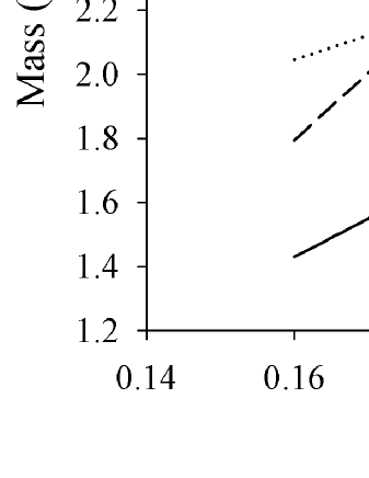
Figure 1: Masses of glueball states $0^{++}$ ($L=S=0$), $2^{++}$ ($L=0,S=2$), and $0^{-+}$ ($L=S=1$) as a function of the string tension $a$, for the model III with $\alpha_{S}=0.5$ and $\gamma=0.52$ GeV^-1.

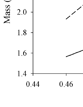
Figure 2: Masses of glueball states $0^{++}$ ($L=S=0$), $2^{++}$ ($L=0,S=2$), and $0^{-+}$ ($L=S=1$) as a function of the gluon size $\gamma$, for the model III with $\alpha_{S}=0.5$ and $a=0.2$ GeV².

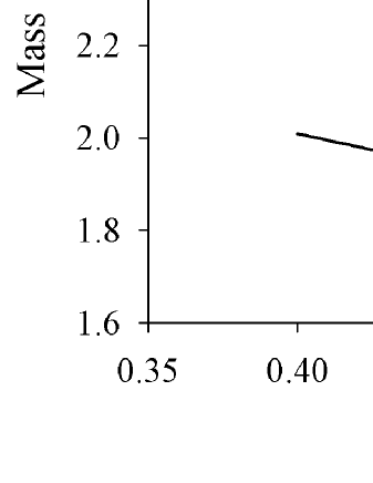
Figure 3: Masses of glueball states $0^{++}$ ($L=S=0$), $2^{++}$ ($L=0,S=2$), and $0^{-+}$ ($L=S=1$) as a function of the strong coupling constant $\alpha_{S}$, for the model III with $a=0.2$ GeV² and $\gamma=0.52$ GeV^-1.

In the models considered below, the gluon masses ($m_{K}$ and $m$) will be fixed by physical considerations. We are then left with 3 parameters: $\alpha_{s}$ (or $\lambda$) for $V_{\text{SR}}$, $\beta$ or $a$ for $V_{\text{conf}}$, and the gluon size $\gamma$ for which less constraints exist on its value. Fortunately, the mass of the lightest $2^{++}$ state is nearly independent of the parameters $\alpha_{s}$ and $\gamma$. For this state, the spin-orbit and diagonal tensor potentials vanish and the two remaining contributions have opposite signs. So, the confinement potential is the largely dominant contribution to this $2^{++}$ mass (see Figs. 1-3). We can fix the value of $\beta$ or $a$ with this state only, knowing that a lattice calculation morn99 and a quasiparticle model szcz03 favor a $2^{++}$ mass around 2.4 GeV, but that some experimental candidates are found around 2 GeV zou99 ; bugg00 . Some agreements between theoretical calculations and experimental data exist about mass ratios of some lightest glueball candidates (see Refs. morn99 ; zou99 ; bugg00 and Table 1): $M(0^{++})/M(2^{++})\sim 0.72-0.78$ and $M(0^{-+})/M(2^{++})\sim 1.10$. So, we will fix the parameters $\alpha_{s}$ and $\gamma$ in order to reproduce at best these mass ratios. Let us note that the mass ratios in lattice calculations can be more interesting quantities to consider than absolute masses, due to the existence of normalization problems morn99 .

III.2 Model I

The first model we consider is by two aspects close to the models of Refs. corn83 and hou03 : The short-range part is supplemented by a saturated confinement potential and the gluon is assumed to be characterized by an unique effective mass $m_{K}=m$, around the typical value of 700 MeV. In this paper, we choose the value of Ref. hou03 . Nevertheless, the model is semirelativistic and the short-range part is not treated perturbatively. The particular characteristics of model I are:

• $m_{K}=m=0.670$ GeV hou03 ;

• $V_{\text{conf}}$ with $W_{\beta}(r)$.

To find a mass of the lightest $2^{++}$ state around 2 GeV, it is necessary to take $\beta\approx 0.2$, which corresponds to $a\approx 0.08$ GeV², a quite unrealistic value. A mass around 2.4 GeV can be obtained with $\beta\approx 0.5$ corresponding to $a\approx 0.2$ GeV², a more realistic value. The parameters $\beta=0.5$, $\alpha_{S}=0.5$, and $\gamma=0.5$ GeV^-1 give the following lightest mass ratios: $M(0^{++})/M(2^{++})=0.93$ and $M(0^{-+})/M(2^{++})=0.73$. Let us note that if the spin-orbit contribution from confinement is not taken into account, the last ratio decreases to 0.61. A lower value for the mass ratio $M(0^{++})/M(2^{++})$ can be obtained by modifying the parameters $\alpha_{S}$ and $\gamma$, but in this case, the mass ratio $M(0^{-+})/M(2^{++})$ also decreases. It can even take negative values for realistic values of the parameters $\alpha_{S}$ and $\gamma$. This nonphysical behavior is due to the spin-orbit potential from $V_{\text{SR}}$ which becomes very attractive. It is worth noting that a variation of the gluon effective mass of 200 MeV around the value 670 MeV does not change noticeably the results. Thus, the model I is not able to describe neither the lightest $2^{++}$ mass state, nor the lightest mass ratios $M(0^{++})/M(2^{++})$ and $M(0^{-+})/M(2^{++})$.

If the channel mixing due the tensor operator is turned on, the situation gets worse. For instance, without channel mixing the lightest $2^{++}$ state ($L=0$, $S=2$) has a reasonable mass. With channel mixing, the $L=0$ component is coupled with $L=2$ and $L=4$ components for which the total spin-orbit contribution is very attractive. The mass of this state becomes then negative, even for realistic values of the parameters $\beta$, $\alpha_{S}$ and $\gamma$.

III.3 Model II

The model II is the same as model I but with the saturated confinement replaced by the linear confinement. The particular characteristics of model II are:

• $m_{K}=m=0.670$ GeV hou03 ;

• $V_{\text{conf}}$ with $W_{a}(r)$.

This model and the previous one give essentially the same results about the lightest mass ratios $M(0^{++})/M(2^{++})$ and $M(0^{-+})/M(2^{++})$. Moreover, masses around 2.4 GeV and 2 GeV are obtained for the lightest $2^{++}$ state with $a\approx 0.12$ GeV² and $a\approx 0.07$ GeV² respectively, quite unrealistic values of the meson string tension.

III.4 Model III

With the two previous models, the spin-orbit effect from the one gluon-exchange is too attractive and cannot be counteracted efficiently by the spin-orbit contribution coming from the confinement. The strength of this attractive potential can be reduced by decreasing the values of $\alpha_{S}$. But in this case, it is not possible to obtain reasonable mass ratios for the lightest $0^{++}$, $2^{++}$, and $0^{-+}$ states. Another possibility is to increase the values of the effective mass $m$. But, if we keep the link $m_{K}=m$, then too high masses are obtained for all glueballs, due to the contribution of the kinetic part of the Hamiltonian. Fortunately, it is physically relevant to choose $m_{K}\ll m$.

For a system of two identical particles with mass $m$, the coefficient $1/m^{2}$ appears naturally in the relativistic corrections of a static potential. A better approximation, proposed in Ref. luch91 and used for instance in Ref. godf85 , is to replace this coefficient by $1/E^{2}(\bm{p})$ where $E(\bm{p})=\sqrt{\bm{p}^{2}+m^{2}}$.

A similar procedure is also proposed within the auxiliary field formalism (also called einbein field formalism) morg99 , which can be considered as an approximate way to handle semirelativistic Hamiltonians sema04 . Within this approach, the effective QCD Hamiltonian for two identical particles (quark or gluon) depends on the current particle mass $m$ and on a state dependent constituent mass $\mu=\sqrt{\langle\bm{p}^{2}+m^{2}\rangle}$ sema04 . All corrections to the static potential are then expanded in powers of $1/\mu^{2}$.

We will adapt these prescriptions in the model III. In principle, the mass appearing in the leading corrections must be replaced by the operator $E(\bm{p})=\sqrt{\bm{p}^{2}+m^{2}}$ where $m$ is the mass appearing in the kinetic operator. This leads to a very complicated nonlocal potential which is very difficult to handle. So we will use an approximation.

Following the hypotheses of Ref. simo00 , we will assume that the gluons are massless and that the dominant effective QCD Hamiltonian $H_{gg}$ for a two-gluon glueball is written

$$H_{gg}=2\sqrt{\bm{p}^{2}}+a_{G}\,r.$$ (12)

The eigenvalues $M_{nL}$ and the constituent masses $\mu_{nL}$ corresponding to this Hamiltonian are in very good approximation given by the following relations simo89 ; sema04

$$M_{nL}=4\mu_{nL}\quad\text{with}\quad\mu_{nL}=\sqrt{a_{G}}\left(\frac{\epsilon_{nL}}{3}\right)^{3/4}.$$ (13)

$\epsilon_{nL}$ is an eigenvalue of the Hamiltonian $\bm{q}^{2}+|\bm{x}|$, in which $\bm{q}$ and $\bm{x}$ are dimensionless conjugate variables. These eigenvalues can be accurately computed with a Lagrange-mesh method for instance baye86 . Let us note that $\epsilon_{n0}$ is the $n$th zero of the Airy function. These constituents masses will then appear in the leading corrections to the dominant hamiltonian $H_{gg}$.

Finally, the particular characteristics of model III are:

• $m_{K}=0$ and $m=\mu_{nL}$ (13);

• $V_{\text{conf}}$ with $W_{a}(r)$.

Let us note that, with our hypotheses, the constituent mass depends on the principal quantum number $n$ of the glueball, on its orbital momentum $L$, but not on the quantum numbers $S$ and $J$.

As mentioned before, we fix the value of the string tension only with the mass of the lightest $2^{++}$ glueball. Equations (13) show that, in first approximation, the mass scale is simply given by $\sqrt{a_{G}}$. By computing a great number of spectra for various parameters, we have remarked that the values of the lightest mass ratios $M(0^{++})/M(2^{++})$ and $M(0^{-+})/M(2^{++})$ cannot be fixed independently. Provided an approximate linear dependence is kept between the two parameters $\alpha$ and $\gamma$, these mass ratios do not change significantly. Finally, we have chosen to present the glueball spectra for two sets of parameters.

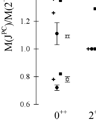
Figure 4: Glueball mass ratios normalized to the lightest $2^{++}$ state (see Table 1). Cross: Set of parameters B for model III; Black circle: Lattice results morn99 ; Black square: Quasiparticle model szcz03 ; White circle: Experiment zou99 ; White square: Experiment bugg00 . The experimental states with a question mark are seen but the uncertainty is not known.

With $a=0.16$ GeV², $\alpha_{S}=0.40$, and $\gamma=0.504$ GeV^-2 (set A), the mass of the lightest $2^{++}$ glueball is 2051 MeV, which is close to some experimental candidates. These values for $a$ and $\alpha_{S}$ are near those used in some recent baryon calculations naro02 . Moreover, the value of the string tension is close to a value found in a recent lattice study taka01 . With $a=0.21$ GeV², $\alpha_{S}=0.50$, and $\gamma=0.495$ GeV^-1 (set B), the mass of the lightest $2^{++}$ glueball is 2384 MeV, which is close to a result obtained with lattice calculations. All results are presented in table 1 and in Fig. 4 with some results from a lattice calculations morn99 and from a quasiparticle approach with no free parameters szcz03 , and with some possible experimental candidates zou99 ; bugg00 .

We can see that the mass ratios for the two sets of parameters are in rather good agreement with the theoretical mass ratios predicted by the lattice study morn99 . Moreover, the absolute masses for set B are within the theoretical error bars of the lattice masses. The largest discrepancy is for the first excited $0^{++}$ glueball, the state predicted by the lattice calculations with the largest error bar.

Our mass ratios are similar to those obtained in the quasiparticle model szcz03 , but are closer to the mass ratios of the lattice studies. It is worth mentioning that this quasiparticle approach contains no free parameters. Again, it favors a 2.4 GeV value for the mass of the lightest $2^{++}$ state, like the lattice model.

The lack of reliable identification of glueballs makes comparison with experimental data more hazardous. The set A results are in rather good agreement with data only for the lightest $0^{++}$, $2^{++}$, and $0^{-+}$ glueball candidates, the states used to fix the parameters. The general tendance of our model and of lattice calculations is to predict excited states with higher masses than those which seem to be observed.

Lattice calculations seem to rule out the presence of $1^{-+}$ and $1^{++}$ states below 4 GeV. This can be qualitatively understood in terms of interpolating operators of minimal dimension which can create glueball states, with the expectation that higher dimensional operators create higher mass states: the lowest states $0^{++}$, $2^{++}$, $0^{-+}$ and $2^{-+}$ are produced by dimension-4 operators, while $1^{++}$ and $1^{-+}$ are respectively produced by dimension-5 and dimension-6 operators morn99 . Nevertheless, our model predicts the existence of $1^{-+}$ and $1^{++}$ states around 3 GeV. In the model of Ref. corn83 , a $1^{-+}$ state is predicted below the $2^{++}$ state (no $1^{++}$ state is mentioned). Possible experimental candidates exist for low mass $1^{++}$ states zou99 , but as mentioned above, the identification is far from certain. The presence of the relatively low mass $1^{-+}$ and $1^{++}$ states in our model may be due to the use of massive valence gluons with three states of polarization (creation of a spin one glueball with two massless gluons, with only two states of polarization, is problematical). In our model III, the gluon is massless in the kinetic part, but a constituent non-zero mass unavoidably appears for the spin corrections simo00 . The presence of spin one states around 3 GeV in our model could indicate what are the limits of a potential approach.

If the spin-orbit contribution from confinement is not taken into account, the agreement between our masses and the lattice results become poorer. For the parameters of set A, the mass ratio for the lightest $0^{-+}$ glueball changes from 1.06 to 0.87, and the mass ratio for the first excited $0^{++}$ glueball changes from 1.26 to 0.83. This shows that the spin-orbit contribution from confinement is an important ingredient of the model.

The channel mixing due to the tensor force is difficult to implement within this model. As $\mu$ depends on the orbital momentum, the diagonal potential for each channel is characterized by a different value of $\mu$. The problem is to define this parameter for the mixing potentials. We have performed several test computations using a mean value of $\mu$ for all channels. This gave us strong indications that the coupling of channels has a small influence on the glueball masses, contrary to the two previous models. We estimate that the masses of the lightest glueballs could be modified by a quantity comprised between 50 and 100 MeV.

IV Conclusion

The masses of pure two-gluon glueballs have been studied with a semirelativistic potential model. The potential is the sum of a one-gluon exchange interaction and a linear confining potential, assumed to be of scalar type. The gluon is massless but the leading corrections of the dominant part of the Hamiltonian are expressed in terms of a state dependent constituent mass. The Hamiltonian depends only on 3 parameters: the strong coupling constant, the string tension, and the gluon size. This last parameter, less constrained than the two others by the QCD theory, removes all singularities in the leading corrections of the potential. These corrections are not treated as perturbations of the dominant part. All masses have been accurately computed with a Lagrange mesh method.

The masses predicted by our potential model are in agreement with experimental glueball candidates only for the lightest $0^{++}$, $2^{++}$, and $0^{-+}$ states zou99 ; bugg00 , but are in rather good agreement with spectra obtained by a lattice calculation morn99 and in reasonable agreement with spectra obtained by a quasiparticle model szcz03 . A notable difference is the presence in our model of spin one states around 3 GeV. This could indicate the limit of the validity for a potential approach.

We have tested other nonrelativistic and semirelativistic potential models in which a constant constituent gluon mass is used, and we have found that it is not possible to obtain good spectra for realistic values of the QCD parameters (see Sec. III.2 and III.3). The main problem arises from the strongly attractive spin-orbit potential for the one-gluon exchange. When its strength is not reduced by a large constituent gluon mass, it can lead to negative nonphysical glueball mass.

The constituent gluon mass is introduced in our model by an approximate procedure which relies on the existence of a pure linear confinement between the gluons simo89 ; sema04 . A more physical ansatz should be to define the constituent mass as a momentum dependent operator ($\sqrt{\bm{p}^{2}}$ for massless gluon) luch91 . It could then be possible to take into account correctly the channel coupling due to the tensor forces, and to use naturally a saturated confinement potential. It could also be interesting to compute three-gluon glueball masses within the same model. Such a work is in progress.

V Acknowledgments

F. Brau (FNRS Postdoctoral Researcher) and C. Semay (FNRS Research Associate) would like to thank the FNRS for financial support.

Appendix A Convolutions

Applied for some useful potentials, the formula (11) gives

$$\widetilde{\delta^{3}}(\bm{r}) = \frac{1}{8\pi\gamma^{3}}e^{-r/\gamma},$$ (14)

$$\widetilde{r} = r+\frac{4\gamma^{2}}{r}\left(1-e^{-r/\gamma}\right)-\gamma e^{-r/\gamma},$$ (15)

$$\widetilde{e^{-ar}} = \frac{4a\gamma^{2}}{(a^{2}\gamma^{2}-1)^{3}}\left(\frac{e^{-ar}}{r}-\frac{e^{-r/\gamma}}{r}\right)+\frac{e^{-ar}+a\gamma\,e^{-r/\gamma}}{(a^{2}\gamma^{2}-1)^{2}},$$ (16)

$$\widetilde{\frac{e^{-ar}}{r}} = \frac{1}{(a^{2}\gamma^{2}-1)^{2}}\left(\frac{e^{-ar}}{r}-\frac{e^{-r/\gamma}}{r}\right)+\frac{e^{-r/\gamma}}{2\gamma(a^{2}\gamma^{2}-1)}.$$ (17)

One can easily verify that $\lim_{\gamma\rightarrow 0}\widetilde{U(r)}=U(r)$ for each potential $U(r)$.

Appendix B Angular momentum operators

A system of two particles, with spin $s_{1}$ and $s_{2}$ respectively, with a total spin $S$ and a total orbital angular momentum $L$ coupled to a total angular momentum $J$, is noted here $|L,S\rangle=|s_{1},s_{2};L,S;J\rangle$. The mean value of the operators $\bm{S}^{2}$ and $\bm{L}\cdot\bm{S}$ are trivial to compute

$$\langle L^{\prime},S^{\prime}|\bm{S}^{2}|L,S\rangle = S(S+1)\,\delta_{L^{\prime},L}\,\delta_{S^{\prime},S},$$ (18)

$$\langle L^{\prime},S^{\prime}|\bm{L}\cdot\bm{S}|L,S\rangle = \frac{1}{2}\Big{[}J(J+1)-L(L+1)-S(S+1)\Big{]}\,\delta_{L,L^{\prime}}\,\delta_{S,S^{\prime}}.$$ (19)

The computation of the mean value of the operator $T$ is much more involved. Using formulas from Ref. vars88 , one can find ($\hat{n}=\sqrt{2n+1}$)

$$\langle L^{\prime},S^{\prime}|T|L,S\rangle = (-1)^{L+L^{\prime}+S^{\prime}+J}\,\hat{S}\hat{S}^{\prime}\hat{L}\hat{L}^{\prime}\left(\begin{array}[]{ccc}L&2&L^{\prime}\\ 0&0&0\end{array}\right)\left\{\begin{array}[]{ccc}S&L&J\\ L^{\prime}&S^{\prime}&2\end{array}\right\}$$ (34)

$$\times\Bigg{[}\phantom{+}(-1)^{S+1+s_{2}-3s_{1}}\,\hat{s}_{1}\sqrt{s_{1}(s_{1}+1)(2s_{1}-1)(2s_{1}+3)}\left\{\begin{array}[]{ccc}s_{1}&s_{2}&S\\ S^{\prime}&2&s_{1}\end{array}\right\}$$

$$\phantom{\times}\phantom{\Bigg{[}}+(-1)^{S+1+s_{1}-3s_{2}}\,\hat{s}_{2}\sqrt{s_{2}(s_{2}+1)(2s_{2}-1)(2s_{2}+3)}\left\{\begin{array}[]{ccc}s_{2}&s_{1}&S\\ S^{\prime}&2&s_{2}\end{array}\right\}$$

$$\phantom{\times}\phantom{\Bigg{[}}-2\sqrt{30}\,\hat{s}_{1}\hat{s}_{2}\sqrt{s_{1}(s_{1}+1)s_{2}(s_{2}+1)}\left\{\begin{array}[]{ccc}s_{1}&s_{2}&S\\ 1&1&2\\ s_{1}&s_{2}&S^{\prime}\end{array}\right\}\Bigg{]}.$$

Table 1: Glueball masses in MeV (mass ratios normalized to lightest $2^{++}$) [$L$ and $S$ quantum numbers only relevant for our model] obtained with model III for two sets of parameters (A: $a=0.16$ GeV², $\alpha_{S}=0.40$, and $\gamma=0.504$ GeV^-1; B: $a=0.21$ GeV², $\alpha_{S}=0.50$, and $\gamma=0.495$ GeV^-1). Some theoretical results from other models and some possible experimental candidates are also indicated. The lightest $0^{++}$, $2^{++}$, and $0^{-+}$ states are taken as inputs to fix the parameters.

$J^{PC}$	Model III			Lattice morn99	Quasiparticle szcz03	Experiment zou99	Experiment bugg00
	[$L$,$S$]	A	B
$0^{++}$	[0,0]	1604 (0.78)	1855 (0.78)	1730$\pm$50$\pm$80 (0.72)	1980 (0.82)		1507$\pm$5 (0.78)
	[2,2]	2592 (1.26)	2992 (1.26)	2670$\pm$180$\pm$130 (1.11)	3260 (1.35)		2105$\pm$15 (1.09)
	[0,0]	2814 (1.37)	3251 (1.36)
$2^{++}$	[0,2]	2051 (1.00)	2384 (1.00)	2400$\pm$25$\pm$120 (1.00)	2420 (1.00)	2020$\pm$50 (1.00)	1934$\pm$12 (1.00)
	[0,2]	2985 (1.46)	3447 (1.45)		3110 (1.29)	2240$\pm$40 (1.11)
	[2,0]	3131 (1.53)	3611 (1.51)			2370$\pm$50 (1.17)
	[2,2]	3230 (1.57)	3695 (1.55)
$0^{-+}$	[1,1]	2172 (1.06)	2492 (1.05)	2590$\pm$40$\pm$130 (1.08)	2220 (0.92)	2140$\pm$30 (1.06)	2190$\pm$50 (1.13)
	[1,1]	3228 (1.57)	3714 (1.56)	3640$\pm$60$\pm$180 (1.52)	3430 (1.42)
$1^{-+}$	[1,1]	2626 (1.28)	3011 (1.26)
	[1,1]	3349 (1.63)	3852 (1.62)
$2^{-+}$	[1,1]	2573 (1.25)	2984 (1.25)	3100$\pm$30$\pm$150 (1.29)	3090 (1.28)	2040$\pm$40 (1.01)
	[1,1]	3345 (1.63)	3862 (1.62)	3890$\pm$40$\pm$190 (1.62)	4130 (1.71)	2300$\pm$40 (1.14)
$1^{++}$	[2,2]	3098 (1.51)	3501 (1.47)			$\sim$ 1700 (0.84)
	[2,2]	3753 (1.83)	4294 (1.80)			2340$\pm$40 (1.16)
$3^{++}$	[2,2]	3132 (1.53)	3611 (1.51)	3690$\pm$40$\pm$180 (1.54)	3330 (1.38)	2000$\pm$40 (0.99)
	[2,2]	3762 (1.83)	4332 (1.82)		4290 (1.77)	2280$\pm$30 (1.13)
$4^{++}$	[2,2]	2897 (1.41)	3360 (1.41)		3990 (1.65)	2044$\pm$? (1.01)
	[2,2]	3633 (1.77)	4197 (1.76)		4280 (1.77)	2320$\pm$30 (1.15)

References

- (1) J. M. Cornwall and A. Soni, Phys. Lett. B 120, 431 (1983).
- (2) W. S. Hou and G. G. Wong, Phys. Rev. D 67, 034003 (2003).
- (3) F. Brau and C. Semay, Comment on “Glueball spectrum from a potential model”, submitted to Phys. Rev. D.
- (4) Yu. A. Simonov, Phys. Lett. 515, 137 (2001).
- (5) W. S. Hou and A. Soni, Phys. Rev. D 29, 101 (1984).
- (6) Yu. A. Simonov, in Proceedings of the XVII Autumn School Lisboa, Portugal, 24 September - 4 October 1999, edited by L. Ferreira, P. Nogueira, and J. I. Silva-Marco (World Scientific, Singapore, 2000), p. 60; hep-ph/9911237.
- (7) W. Lucha, F. F. Schöberl, and D. Gromes, Phys. Rep. 200, 127 (1991).
- (8) W. S. Hou, C. S. Luo, and G. G. Wong, Phys. Rev. D 64, 014028 (2001).
- (9) F. Brau and C. Semay, Phys. Rev. D 58, 034015 (1998).
- (10) F. Brau, C. Semay, and B. Silvestre-Brac, Phys. Rev. C 66, 055202 (2002).
- (11) B. Silvestre-Brac, F. Brau, and C. Semay, J. Phys. G: Nucl. Part. Phys. 29, 2685 (2003).
- (12) F. Brau, Thesis, Université de Mons-Hainaut, 2001 (unpublished).
- (13) C. Semay and B. Silvestre-Brac, Phys. Rev. D 46, 5177 (1992).
- (14) L. P. Fulcher, Phys. Rev. D 50, 447 (1994).
- (15) D. Baye and P.-H. Heenen, J. Phys. A 19, 2041 (1986); D. Baye, J. Phys. B 28, 4399 (1995).
- (16) C. Semay, D. Baye, M. Hesse, and B. Silvestre-Brac, Phys. Rev. E 64, 016703 (2001).
- (17) C. J. Morningstar and M. J. Peardon, Phys. Rev. D 60, 034509 (1999).
- (18) A. P. Szczepaniak and E. S. Swanson, Phys. Lett. B 577, 61 (2003).
- (19) B. S. Zou, Nucl. Phys. A655, 41 (1999).
- (20) D. V. Bugg, M. J. Peardon, and B. S. Zou, Phys. Lett. B 486, 49 (2000).
- (21) S. Godfrey and N. Isgur, Phys. Rev. D 32, 189 (1985).
- (22) V. L. Morgunov, A. V. Nefediev, and Yu. A. Simonov, Phys. Lett. B 459, 653 (1999).
- (23) C. Semay, B. Silvestre-Brac, and I. M. Narodetskii, Phys. Rev. D 69, 014003 (2004).
- (24) Yu. A. Simonov, Phys. Lett. B 226, 151 (1989).
- (25) I. M. Narodetskii and M. A. Trusov, Yad. Fiz. 65, 949 (2002); Phys. Atom. Nucl. 65, 917 (2002); Phys. Atom. Nucl. 66 (2003), in print, hep-ph/0307131
- (26) T. T. Takahashi, H. Matsufuru, Y. Nemoto, and H. Suganuma, Phys. Rev. Lett. 86, 18 (2001); Phys. Rev. D 65, 114509 (2002).
- (27) D. A. Varshalovich, A. N. Moskalev, and V. K. Khersonskii, Quantum Theory of Angular Momentum (World Scientific, Singapore, 1988).