Twistor-Inspired Construction of Electroweak Vector Boson Currents

Abstract

We present an extension of the twistor-motivated MHV vertices and accompanying rules presented by Cachazo, Svrček and Witten to the construction of vector-boson currents coupling to an arbitrary source. In particular, we give rules for constructing off-shell vector-boson currents with one fermion pair and $n$ gluons of arbitrary helicity. These currents may be employed directly in the computation of electroweak amplitudes. The rules yield expressions in agreement with previously-obtained results for $Z,W,\gamma^{*}\rightarrow{\overline{\kern-0.7ptq\kern-0.7pt}}q+n$ gluons (analytically up to $n=3$, beyond via the Berends–Giele recursion relations). We also confirm that the contribution to a seven-point amplitude containing the non-abelian triple vector-boson coupling obtained using the next-to-MHV currents matches the previous result in the literature.

I Introduction

Computations of amplitudes in gauge theories play an essential role in probing beyond the Standard Model of particle physics interactions. The short-distance experimental environment at hadron colliders forces us to consider numerous processes with QCD interactions. Electroweak gauge bosons have played, and will likely play, an important role as experimentally distinctive probes of new physics. Both QCD and mixed electroweak-QCD processes contribute important backgrounds to various new-physics signals. The computation of amplitudes for such processes is thus an important part of a physics program at modern-day colliders.

At tree-level, an elegant — and computationally-efficient — approach was found a decade and a half ago by Berends and Giele Recurrence . Other related approaches have also been employed OtherNumerical . In addition, various computer-driven approaches such as MADGRAPH Madgraph , are widely used.

These approaches are not the end of the story, however. For QCD and other massless gauge theories, Cachazo, Svrček and Witten (CSW) CSW have presented a powerful set of new computational rules for scattering amplitudes. These rules emerged from analyses inspired by Witten’s WittenTopologicalString proposal of a weak–weak coupling duality between ${\cal N}=4$ supersymmetric gauge theory and the topological open-string $B$ model with a twistor target space. This proposal generalizes Nair’s earlier description Nair of the simplest gauge-theory amplitudes. (Berkovits and Motl Berkovits ; BerkovitsMotl , Neitzke and Vafa Vafa , and Siegel Siegel have given alternative descriptions of such a possible topological dual to the ${\cal N}=4$ theory.) The CSW rules are of interest in their own right for tree-level computations. Their efficiency can be improved when recast in a recursive form MHVRecursive (dual in a sense to ‘connected’ twistor space prescriptions Gukov ). They also show great promise for simplifying loop calculations TwistorLoop . (A direct topological-string approach appears to be problematic because of the appearance of non-unitary states from conformal supergravity BerkovitsWitten .) Our purpose here is to extend the CSW construction to include building blocks for mixed QCD-electroweak amplitudes.

Witten’s weak–weak duality is a very promising step towards understanding why amplitudes in unbroken gauge theories are so much simpler than expected from the Feynman diagram expansion. The best-known example of simplicity in amplitudes is given by the Parke–Taylor amplitudes ParkeTaylor of massless gauge theories (including, of course, QCD). These are an infinite series of amplitudes, with two negative-helicity gluons and an arbitrary number of positive-helicity ones (or their parity conjugates). They are usually called ‘maximally helicity-violating’ (MHV) amplitudes. They play an important role in the CSW construction, as the vertices are a particular off-shell continuation of the MHV amplitudes. Although no-one has as yet given a direct derivation of the CSW diagrams from a Lagrangian there is little doubt they are correct, because they exhibit the correct kinematic poles and maintain Lorentz invariance, although it is not manifest CSW . The rules extend to any massless gauge theory Khoze , and lead to explicit results for next-to-MHV amplitudes CSW ; Khoze ; NMHVTree , and have undergone non-trivial checks using ‘googly’ amplitudes (the parity conjugates of the MHV amplitudes) in the context of string and field theory RSV1 ; OtherGoogly ; WittenParity . The CSW rules or their recursive reformulation can be implemented either analytically or numerically.

The twistor-motivated constructions to date have largely left unaddressed the question of how to compute processes which contain both colored and uncolored particles. Of particular importance to collider experiments are of course the computation of amplitudes with both QCD and electroweak particles. Dixon, Glover, and Khoze LanceHiggs took the first step in this direction, in showing how to compute amplitudes containing a Higgs boson coupled to QCD via a massive top-quark loop (in the infinite-mass limit). Our purpose here is to incorporate another important class of processes, those containing electroweak vector bosons.

We will do so by providing a CSW-like construction of vector currents, which may in principle be coupled to an arbitrary source. Typically, one is interested in processes where produced vector bosons decay into lepton pairs. For this purpose, one would couple the currents to lepton pairs. However, one can also couple them to more complicated electroweak objects, including, for example, non-abelian currents decaying in turn into combinations of Higgs bosons and multiple lepton pairs. These applications go beyond the CSW construction, and are a step in the direction of constructing an off-shell effective action $\Gamma[A]$.

We will focus on the case of coupling a process involving one quark pair and any number of gluons to one colorless off-shell vector boson. The constructions should generalize, however, to processes with multiple quark pairs, and presumably to those with any number of electroweak gauge bosons. Indeed, as we shall discuss, the generalization to symmetrized electroweak gauge bosons ($Z,\gamma^{*}$) is straightforward. It should also be possible to construct similar currents for colored vector bosons, but we will defer a discussion of these issues to future papers. The key idea in the construction is to introduce a new set of basic vertices coupling to the off-shell vector boson, analogous to the MHV vertices of CSW. These basic vertices have either one or no negative-helicity gluons. The rules for combining them into new currents with additional negative-helicity legs are then in fact the same as those of CSW.

While we will not provide a first-principles proof of our construction of the vector boson currents, we shall display considerable evidence that it is correct. It exhibits the correct factorization properties on kinematic poles. It agrees with previously-computed amplitudes. In particular, in Appendix C of ref. BGKVectorBoson vector boson currents for $Z,W,\gamma^{*}\rightarrow{\overline{\kern-0.7ptq\kern-0.7pt}}q+n$ gluons up to $n=3$ are given and we find complete agreement. We have also implemented a light-cone gauge version of the Berends-Giele recursion relations Recurrence ; LightConeRecursion and have compared our new construction numerically with currents computed thereby up to six gluons of any helicity and eight gluons with selected helicities.

This paper is organized as follows. In section II, we review color decompositions, especially for the case of vector boson exchange. In section III, we review helicity and MHV vertices. In section IV, we generalize MHV vertices to vertices for currents. The properties of the amplitudes, including various consistency checks are discussed in section V. Finally, in section VI, we give our conclusions and outlook.

II Review of Color Decompositions with Vector Bosons

It is convenient to write the full momentum-space amplitudes using color decompositions TreeColor ; TreeReview . For example, the tree-level $n$-gluon amplitude ${\cal A}_{n}$ has the color decomposition,

$${\cal A}_{n}(1,2,\ldots,n)=\sum_{\sigma\in S_{n}/Z_{n}}\,{\rm Tr}(T^{a_{\sigma(1)}}\cdots T^{a_{\sigma(n)}})\,A_{n}(\sigma(1),\ldots,\sigma(n)))\,,$$ (1)

where $S_{n}/Z_{n}$ is the group of non-cyclic permutations on $n$ symbols, and $j$ denotes the $j$-th gluon and its associated momentum. For now we are suppressing the helicity labels. We use the color normalization $\,{\rm Tr}(T^{a}T^{b})=\delta^{ab}$. Similar decompositions hold for cases involving quarks. In general, it is more convenient to calculate the partial amplitudes than the entire amplitude at once.

The cases in which we are interested here involve colorless vector bosons. Though it may seem surprising at first sight, single massive vector boson exchange is easily obtained from pure QCD amplitudes (which are directly calculable from CSW diagrams). For example, for ${e^{+}}{{e^{-}}}\rightarrow\gamma^{*}\rightarrow q{\overline{\kern-0.7ptq\kern-0.7pt}}+n$ gluons, where $\gamma^{*}$ represents an off-shell photon, the amplitude reduces to

$$\hbox{}\hskip-14.22636pt{\cal A}_{n}(1_{e^{+}},2_{{e^{-}}},3_{q},4,5,\ldots,(n-1),n_{\overline{\kern-0.7ptq\kern-0.7pt}}) = -2e^{2}Q^{q}g^{n-2}\sum_{\sigma\in S_{n-4}}(T^{a_{\sigma}(4)}T^{a_{\sigma}(5)}\cdots T^{a_{\sigma}(n-1)})_{i_{3}}^{\;{\bar{\imath}}_{n}}$$ (2)

$$\hskip 2.84544pt\hbox{}\times A_{n}(1_{e^{+}},2_{{e^{-}}},3_{q},\sigma(4),\sigma(5),\ldots,\sigma(n-1),n_{\overline{\kern-0.7ptq\kern-0.7pt}})\,,$$

where we use an all outgoing momentum convention. The particle labels $q,{\overline{\kern-0.7ptq\kern-0.7pt}},{{e^{-}}},{e^{+}}$ signify quarks, anti-quarks, electrons and positrons, while legs without labels signify gluons. The off-shell photon, is internal to the amplitude and exchanged between the lepton pair and the quark pair.

One may then convert the exchanged photon to an electroweak vector boson very simply by adjusting the coupling and modifying the photon kinematic pole to be the appropriate one for an unstable massive particle (see, for example, BGKVectorBoson ; DKS ). In particular, for $e^{+}e^{-}\rightarrow Z,\gamma^{*}\rightarrow{\overline{\kern-0.7ptq\kern-0.7pt}}q+ng$ one simply modifies the coefficient in eq. (2) to,

$$Q^{q}\rightarrow Q^{q}-v_{L,R}^{e}v_{L,R}^{q}\,{\cal P}_{Z}(s_{12})\,,$$ (3)

where $s_{12}=(k_{1}+k_{2})^{2}$,

$${\cal P}_{Z}(s_{12})={s_{12}\over s_{12}-M_{Z}^{2}+i\,\Gamma_{Z}\,M_{Z}}\,,$$ (4)

and $M_{Z}$ and $\Gamma_{Z}$ are the mass and width of the $Z$ boson. With the replacement (3), both $Z$ boson and photon exchange are accounted for in eq. (2). The left- and right-handed couplings of fermions to the $Z$ boson are

$$v_{L}^{e} = {-1+2\sin^{2}\theta_{W}\over\sin 2\theta_{W}}\,,\hskip 65.44142ptv_{R}^{e}={2\sin^{2}\theta_{W}\over\sin 2\theta_{W}}\,,$$

$$v_{L}^{q} = {\pm 1-2Q^{q}\sin^{2}\theta_{W}\over\sin 2\theta_{W}}\,,\hskip 54.06006ptv_{R}^{q}=-{2Q^{q}\sin^{2}\theta_{W}\over\sin 2\theta_{W}}\,,$$ (5)

where $\theta_{W}$ is the Weinberg angle. The two signs in $v_{L,R}^{q}$ correspond to up $(+)$ and down $(-)$ type quarks. The subscripts $L$ and $R$ refer to whether the particle to which the $Z$ couples is left- or right-handed. That is, $v_{R}^{q}$ is to be used for the configuration where the quark (leg 3) has plus helicity and the anti-quark (leg $n$) has minus helicity. Similarly, $v_{L}^{q}$ corresponds to the opposite configuration. For $W$ boson exchange, the propagator correction is

$${\cal P}_{W}(s_{12})={s_{12}\over s_{12}-M_{W}^{2}+i\,\Gamma_{W}\,M_{W}}\,,$$ (6)

$M_{W}$ and $\Gamma_{W}$ are the mass and width of the $W$ boson, and the corresponding couplings are,

$$v_{R}^{f_{1}\!f_{2}}=0\,,\hskip 56.9055ptv_{L}^{f_{1}\!f_{2}}={1\over\sqrt{2}\sin\theta_{W}}U_{f_{1}\!f_{2}}\,.\$$ (7)

In the last formula, for quarks $U_{f_{1}\!f_{2}}$ is the Cabibbo-Kobayashi-Maskawa mixing matrix and $f_{1}$ is an up type quark and $f_{2}$ a down type quark. For leptons it is the identity matrix with $f_{1}$ an up type lepton and $f_{2}$ a down type lepton.

More generally, one may convert gluons to photons, purely by group theoretic rearrangements. (As one example of this, see the fourth appendix of ref QQGGG .) However, in general, it is not possible to then convert the photonic amplitudes to ones involving electroweak vector bosons since vector bosons have non-abelian self interactions which photons do not. Although it is rather pleasing that the CSW formalism applies directly to single massive vector boson exchange, cases involving two or more vector bosons are much richer both from phenomenological and theoretical vantage points. A purpose of this paper is to construct an appropriate off-shell continuation so that the CSW methodology can be applied to such cases as well.

III Review of CSW Diagrams

The CSW construction CSW builds amplitudes out of vertices which are off-shell continuations of the Parke–Taylor amplitudes. These amplitudes, with two negative-helicity gluons and any number of positive-helicity ones, are the maximally helicity-violating (MHV) non-vanishing tree-level amplitudes in a gauge theory. In the spinor helicity SpinorHelicity ; XZC ; TreeReview notation, they are,

$$A_{n}(1^{+},\ldots,m_{1}^{-},(m_{1}\!+\!1)\vphantom{1}^{+},\ldots,m_{2}^{-},(m_{2}\!+\!1)\vphantom{1}^{+},\ldots,n^{+})=i{\left\langle m_{1}\,m_{2}\right\rangle^{4}\over\left\langle 1\,2\right\rangle\left\langle 2\,3\right\rangle\cdots\left\langle(n\!-\!1)\,n\right\rangle\left\langle n\,1\right\rangle},$$ (8)

where the two negative-helicity gluons are labeled $m_{1,2}$. In this equation, $\left\langle i\,j\right\rangle=\left\langle k_{i}\,k_{j}\right\rangle$. We follow the standard spinor normalizations $\left[i\,j\right]={\mathop{\rm sign}\nolimits}(k_{i}^{0}k_{j}^{0})\left\langle j\,i\right\rangle^{*}$ and $\left\langle i\,j\right\rangle\left[j\,i\right]=2k_{i}\cdot k_{j}$. With our conventions all particle momenta are taken to be outgoing.

The remaining MHV fermionic amplitudes needed for our discussion of vector boson currents are,

$$A(1_{q}^{+},2^{+},3^{+},\ldots,i^{-},\ldots,(n-2)^{+},(n-1)_{\overline{\kern-0.7ptq\kern-0.7pt}}^{-},n^{+})=i{\left\langle i\,1\right\rangle\left\langle i,\,\,n-1\right\rangle^{3}\over\left\langle 1\,2\right\rangle\left\langle 2\,3\right\rangle\left\langle 3\,4\right\rangle\cdots\left\langle n\,1\right\rangle}\,,$$ (9)

$$A(1_{q}^{+},2^{+},3^{+},\ldots,(n-2)^{+},(n-1)_{\overline{\kern-0.7ptq\kern-0.7pt}}^{-},n^{-})=i{\left\langle n\,1\right\rangle\left\langle n-1,\,\,n\right\rangle^{3}\over\left\langle 1\,2\right\rangle\left\langle 2\,3\right\rangle\left\langle 3\,4\right\rangle\cdots\left\langle n\,1\right\rangle}\,,$$ (10)

$$A(1_{{\overline{\kern-0.7ptq\kern-0.7pt}}^{\prime}}^{-},2_{q^{\prime}}^{+},3_{q}^{+},4^{+},\ldots,(n-1)^{+},n_{\overline{\kern-0.7ptq\kern-0.7pt}}^{-})=-i{\left\langle 1\,n\right\rangle^{2}\over\left\langle 1\,2\right\rangle\left\langle 3\,4\right\rangle\left\langle 4\,5\right\rangle\cdots\left\langle(n-1)\,n\right\rangle}\,.\hskip 28.45274pt$$ (11)

The last equation gives the color-ordered amplitude appearing in eq. (2) after relabeling $q^{\prime}\rightarrow{{e^{-}}}$ and ${\overline{\kern-0.7ptq\kern-0.7pt}}^{\prime}\rightarrow{e^{+}}$. These amplitudes may be obtained from the purely gluonic MHV ones using supersymmetry identities SWI .

In the CSW construction a particular off-shell continuation of these amplitudes is an MHV vertex. The original CSW prescription for the off-shell continuation of a momentum $k_{j}$ amounts to replacing

$$\left\langle j\,j^{\prime}\right\rangle\longrightarrow\left[\eta\,j\right]\left\langle j\,j^{\prime}\right\rangle\longrightarrow\left\langle\smash{\eta}{\vphantom{1}}^{+}\right|{{\raise 0.97221pt\hbox to5.52084pt{\hss/\hss}\hbox to0.0pt{\hss$k$}}_{j}}\left|\smash{j^{\prime}}{\vphantom{1}}^{+}\right\rangle,$$ (12)

where $\eta$ is an arbitrary light-like reference vector, in the Parke-Taylor formula. The extra factors introduced in this off-shell continuation cancel when sewing together vertices to obtain an on-shell amplitude. As shown by CSW CSW , on-shell amplitudes are in fact independent of the choice of $\eta$, implying that the sum over MHV diagrams is Lorentz invariant.

In this paper we use an alternative, but equivalent way of going off-shell NMHVTree ; MHVRecursive . We instead decompose an off-shell momentum $K$ into a sum of two massless momenta, where one is proportional to the auxiliary light-cone reference momentum $\eta$ (with $\eta^{2}=0$),

$$K=k^{\flat}+\zeta(K)\eta\,.$$ (13)

The constraint $(k^{\flat})^{2}=0$ yields

$$\zeta(K)={K^{2}\over 2\eta\cdot K}.$$ (14)

If $K$ goes on shell, $\zeta$ vanishes. Also, if two off-shell vectors sum to zero, $K_{1}+K_{2}=0$, then so do the corresponding $k^{\flat}$s. The prescription for continuing MHV amplitudes or vertices off shell is to replace,

$$\left\langle j\,j^{\prime}\right\rangle\rightarrow\left\langle\smash{j^{\flat}}\,j^{\prime}\right\rangle,$$ (15)

when $k_{j}$ is taken off shell. In the on-shell limit, $\zeta(K)$ vanishes and $k_{j}^{\flat}\rightarrow k_{j}$. Although equivalent to the original CSW prescription, it is a bit more convenient to implement. In particular, there are no extra factors associated with going off-shell and the MHV vertices carry the same dimensions as amplitudes.

The CSW construction replaces ordinary Feynman diagrams with diagrams built out of MHV vertices and ordinary propagators. Each vertex has exactly two lines carrying negative helicity (which may be on or off shell), and at least one line carrying positive helicity. The propagator takes the simple form $i/K^{2}$, because the physical state projector is effectively supplied by the vertices.

We will denote the projected $k^{{\flat}}$ momentum built out of $K=k_{1}+\cdots k_{j}$ by $K^{\flat}$, for example $\left\langle j\,k^{\flat}(K,\eta)\right\rangle=\left\langle j\,K^{\flat}\right\rangle$. For example, with this notation an all-gluon vertex would be,

$$V(1^{+},\ldots,m_{1}^{-},(m_{1}\!+\!1)\vphantom{1}^{+},\ldots,n,K\vphantom{1}^{-})\ =i\,{\left\langle\smash{m_{1}}\,\smash{K^{\flat}}\right\rangle^{4}\over\left\langle 1\,2\right\rangle\left\langle 2\,3\right\rangle\cdots\left\langle\smash{n}\,\smash{K^{\flat}}\right\rangle\left\langle\smash{K^{\flat}}\,\smash{1}\right\rangle}\,.$$ (16)

For the fermionic vertices, there is a subtlety. In the standard phase convention, the on-shell amplitudes have the following sort of expression,

$$A(1^{+},\ldots,f_{1}^{+}\ldots,m_{1}^{-},(m_{1}\!+\!1)\vphantom{1}^{+},\ldots,n,f_{2}\vphantom{1}^{-})\ =i\,{\left\langle m_{1}\,f_{2}\right\rangle^{3}\left\langle m_{1}\,f_{1}\right\rangle\over\left\langle 1\,2\right\rangle\left\langle 2\,3\right\rangle\cdots\left\langle n\,f_{2}\right\rangle\left\langle f_{2}\,1\right\rangle}\,.$$ (17)

In the CSW approach, the helicity projector in the propagator — /$k$ in the fermionic case — is supplied by the vertices. In the amplitude, each momentum is directed outwards. When we attempt to link two vertices, we would obtain $|k_{1}^{+}\rangle\langle k_{2}^{+}|$, for example, from the numerators. This is not the correct form, because $k_{1}=-k_{2}$. Up to an overall sign, what we want is $|k_{2}^{+}\rangle\langle k_{2}^{+}|=|(-k_{1})^{+}\rangle\langle k_{2}^{+}|$. That is, both vertices must have the same momentum argument in the spinor products. To correct this, we must flip the sign of either the positive- or negative-helicity fermion’s momentum in the arguments to the spinor products. We will choose to flip that of the negative-helicity fermion, so that the vertex reads,

$$V(1^{+},\ldots,f_{1}^{+},\ldots,m_{1}^{-},(m_{1}\!+\!1)\vphantom{1}^{+},\ldots,n,f_{2}\vphantom{1}^{-}) = -i\,{\left\langle m_{1}\,(-f_{2})\right\rangle^{3}\left\langle m_{1}\,f_{1}\right\rangle\over\left\langle 1\,2\right\rangle\left\langle 2\,3\right\rangle\cdots\left\langle n\,(-f_{2})\right\rangle\left\langle(-f_{2})\,1\right\rangle}\hskip 36.98866pt$$ (18)

$$= {\mathop{\rm sign}\nolimits}(k_{f_{2}}^{0})\,{\left\langle m_{1}\,f_{2}\right\rangle^{3}\left\langle m_{1}\,f_{1}\right\rangle\over\left\langle 1\,2\right\rangle\left\langle 2\,3\right\rangle\cdots\left\langle n\,f_{2}\right\rangle\left\langle f_{2}\,1\right\rangle}\,,$$

where as usual legs are continued off shell by replacing $k_{j}$ with $k_{j}^{\flat}$, and where $-f_{2}$ denotes $-k_{f_{2}}$. This issue can be ignored in the gluonic vertex because there the corresponding factor would involve ${\mathop{\rm sign}\nolimits}^{2}(k^{0})=1$.

The CSW rules using these vertices will yield fermionic amplitude with a different phase convention than the standard one TreeReview . To obtain the standard phase conventions, we must multiply the on-shell amplitude emerging from the CSW rules by a factor of $i{\mathop{\rm sign}\nolimits}(k^{0})$ for the negative-helicity fermion leg.

The CSW rules then instruct us to write down all tree diagrams with MHV vertices, subject to the constraints that each vertex has exactly two negative-helicity gluons and at least one positive-helicity gluon attached, and that each propagator connects legs of opposite helicity. For amplitudes with two negative-helicity gluons, the vertex with all legs taken on shell is then the amplitude. For each additional negative-helicity gluon, we must add a vertex and a propagator. The number of vertices is thus the number of negative-helicity gluons, less one.

Figure 1: The stripped diagrams for 3 minus helicity amplitudes with vector boson exchange between two fermion pairs. Legs 1 and 2 correspond to the leptons and the legs 3 and $n$ to the quarks. Lines with arrows represent quarks and those without arrows represent either vector bosons or gluons.

As a simple example we may use the CSW rules to construct next-to-MHV (NMHV) partial amplitudes needed for the process $e^{+}e^{-}\rightarrow\gamma^{*},Z,W\rightarrow q\bar{q}+ng$. The ‘stripped diagrams’ for this process are shown in fig. 1. By stripped diagrams, we mean CSW diagrams which have been stripped of all the positive helicity gluons. Dressing the diagrams with the positive helicity gluon legs between $q$ and ${\overline{\kern-0.7ptq\kern-0.7pt}}$ in the color ordering leads to

$$\hskip-11.38092ptA(1_{q^{\prime}}^{-},2_{{\overline{\kern-0.7ptq\kern-0.7pt}}^{\prime}}^{+},3_{q}^{+},4^{+},5^{+},\ldots,(n-1)^{-},n_{\overline{\kern-0.7ptq\kern-0.7pt}}^{-})$$

$$\hskip 48.36958pt=\sum_{j=4}^{n-1}V(1_{q^{\prime}}^{-},2_{{\overline{\kern-0.7ptq\kern-0.7pt}}^{\prime}}^{+},3_{q}^{+},4^{+},5^{+},\ldots,(j-1)^{+},(-K_{1\ldots(j-1)})_{\overline{\kern-0.7ptq\kern-0.7pt}}^{-})\,{i\over K_{1\ldots(j-1)}^{2}}$$

$$\hskip 76.82234pt\hbox{}\times V((-K_{j\ldots n})_{q}^{+},j^{+},\ldots,(n-2)^{+},(n-1)^{-},n_{\overline{\kern-0.7ptq\kern-0.7pt}}^{-})$$

$$\hskip 48.36958pt\hbox{}+\sum_{j=4}^{n-2}V(1_{q^{\prime}}^{-},2_{{\overline{\kern-0.7ptq\kern-0.7pt}}^{\prime}}^{+},3_{q}^{+},4^{+},5^{+},\ldots,(j-1)^{+},(-K_{n,1\ldots(j-1)})^{+},n_{\overline{\kern-0.7ptq\kern-0.7pt}}^{-})\,{i\over K_{n,1\ldots(j-1)}^{2}}$$

$$\hskip 76.82234pt\hbox{}\times V((-K_{j\ldots(n-1)})^{-},j^{+},\ldots,(n-2)^{+},(n-1)^{-})$$

$$\hskip 48.36958pt\hbox{}+V(1_{q^{\prime}}^{-},2_{{\overline{\kern-0.7ptq\kern-0.7pt}}^{\prime}}^{+},(-K_{1,2,n})_{q}^{+},n_{\overline{\kern-0.7ptq\kern-0.7pt}}^{-})\,{i\over K_{n,1,2}^{2}}\,$$ (19)

$$\hskip 76.82234pt\hbox{}\times V(3_{q}^{+},4^{+},\ldots,(n-2)^{+},(n-1)^{-},(-K_{3\ldots(n-1)})_{\overline{\kern-0.7ptq\kern-0.7pt}}^{-})$$

$$\hskip 48.36958pt\hbox{}+V(1_{q^{\prime}}^{-},2_{{\overline{\kern-0.7ptq\kern-0.7pt}}^{\prime}}^{+},(-K_{1,2})^{-})\,{i\over K_{1,2}^{2}}\,V(3_{q}^{+},4^{+},\ldots,(n-2)^{+},(n-1)^{-},n_{\overline{\kern-0.7ptq\kern-0.7pt}}^{-},(-K_{3,\ldots,n})^{+})\,,$$

where $K_{i\ldots j}=k_{i}+k_{i+1}+\cdots+k_{j}$. Renaming ${\overline{\kern-0.7ptq\kern-0.7pt}}^{\prime},q^{\prime}\rightarrow{e^{+}},{e^{-}}$ gives the partial amplitudes appearing in the vector boson exchange amplitudes (2). As discussed above, we must multiply by a factor of $i{\mathop{\rm sign}\nolimits}(k_{n}^{0})$ to obtain the standard phase conventions.

CSW diagrams can be used to obtain any tree-level massless gauge theory amplitude Khoze . As the number of negative helicity legs increases, the complexity of the diagrams increases rapidly. As discussed in ref. MHVRecursive , this growth may be tamed using the recursive rearrangement of diagrams in terms of non-MHV vertices.

In general, using these amplitudes we may obtain single vector boson exchange amplitudes by making modifications to the couplings, color sums and vector boson propagators of the type discussed in section II. However, if we wish to apply the formalism to the phenomenologically interesting cases of vector bosons decaying into Higgs bosons or multiple fermion pairs including the non-abelian vector boson self-coupling, an extension of the formalism is required. In the next section we describe such an extension.

IV MHV Vertices for Vector Boson Currents

In this section we generalize the CSW construction to allow couplings to arbitrary sources. We focus on the phenomenologically interesting case of vector boson currents, though our construction of currents is applicable more generally.

An important application of these currents is that they allow us to couple the electroweak theory to QCD, while taking full advantage of the CSW formalism on the QCD side. The currents satisfy a similar color decomposition as the photon exchange amplitude (2),

$$\hbox{}\hskip-14.22636pt{\cal J}_{\mu}(1_{q},2,3,\ldots,(n-1),n_{\overline{\kern-0.7ptq\kern-0.7pt}};P_{V}) = g_{V}\,g^{n}\sum_{\sigma\in S_{n-2}}(T^{a_{\sigma}(2)}T^{a_{\sigma}(3)}\cdots T^{a_{\sigma}(n-1)})_{i_{1}}^{\;{\bar{\imath}}_{n}}$$ (20)

$$\hskip 2.84544pt\hbox{}\times J_{\mu}(1_{q},\sigma(2),\sigma(3),\ldots,\sigma(n-1),n_{\overline{\kern-0.7ptq\kern-0.7pt}};P_{V})\,,$$

where $g_{V}$ is the appropriate coupling for a vector boson $V=\gamma^{*},Z,W$ and $P_{V}$ is the momentum carried by the vector boson. Hence we need consider only the partial currents $J_{\mu}$ in much the same way that we need only consider color-ordered partial amplitudes.

We start by defining two currents that will serve as new basic vertices for obtaining general vector boson currents:

1. A vector-boson current with $n$ gluon emissions, all of positive helicity

   $$\hbox{}\hskip-14.22636ptJ^{\mu}(1_{q}^{-},2^{+},\ldots,(n-1)^{+},n_{\overline{\kern-0.7ptq\kern-0.7pt}}^{+};P_{V}) = -{i\over\sqrt{2}}{\left\langle\smash{(-1)}{\vphantom{1}}^{-}\right|{\gamma^{\mu}{\raise 0.91666pt\hbox to7.80904pt{\hss/\hss}\hbox to0.0pt{\hss$P$}}_{V}}\left|\smash{(-1)}{\vphantom{1}}^{+}\right\rangle\over\left\langle(-1)\,2\right\rangle\left\langle 2\,3\right\rangle\ldots\left\langle(n-1)\,n\right\rangle}$$ (21)

   $$= c_{+}\,\varepsilon^{(+)\mu}(P_{V}^{\flat},\eta)+c_{-}\,\varepsilon^{(-)\mu}(P_{V}^{\flat},\eta)$$

   $$\hskip 14.22636pt\hbox{}+c_{L}\,\biggl{(}P_{V}^{\mu}-{P_{V}^{2}\over\eta\cdot P_{V}}\eta^{\mu}\biggl{)}\,,\hskip 85.35826pt$$

   where $P_{V}=-K_{1\ldots n}$ by momentum conservation, where ‘$-1$’ as a spinor argument denotes $-k_{1}$, and where

   $$c_{+} = -V^{\rm MHV}(1_{\overline{\kern-0.7ptq\kern-0.7pt}}^{-},\ldots,n_{q}^{+};P_{V}^{-})\,,$$

   $$c_{-} = V^{\rm MHV}(1_{\overline{\kern-0.7ptq\kern-0.7pt}}^{-},\ldots,n_{q}^{+};P_{V}^{-})\,{\left\langle 1\,\eta\right\rangle^{2}P_{V}^{2}\over\left\langle\smash{\eta}\,\smash{P_{V}^{\flat}}\right\rangle^{2}\left\langle\smash{1}\,\smash{P_{V}^{\flat}}\right\rangle^{2}}\,,$$ (22)

   $$c_{L} = V^{\rm MHV}(1_{\overline{\kern-0.7ptq\kern-0.7pt}}^{-},\ldots,n_{q}^{+};P_{V}^{-})\,{\sqrt{2}\left\langle 1\,\eta\right\rangle\over\left\langle\smash{\eta}\,\smash{P_{V}^{\flat}}\right\rangle\left\langle\smash{1}\,\smash{P_{V}^{\flat}}\right\rangle}\,.$$

   The vertex $V^{\rm MHV}$ is simply a CSW vertex for one photon, one quark pair, and $n-2$ gluons, obtained by fermionic phase adjustments from the amplitude in eq. (10).

   If the helicity assignments of the fermions are reversed we instead have

   $$\hbox{}\hskip-14.22636ptJ^{\mu}(1_{q}^{+},2^{+},\ldots,(n-1)^{+},n_{\overline{\kern-0.7ptq\kern-0.7pt}}^{-};P_{V})=-{i\over\sqrt{2}}{\left\langle\smash{(-n)}{\vphantom{1}}^{-}\right|{\gamma^{\mu}{\raise 0.91666pt\hbox to7.80904pt{\hss/\hss}\hbox to0.0pt{\hss$P$}}_{V}}\left|\smash{(-n)}{\vphantom{1}}^{+}\right\rangle\over\left\langle 1\,2\right\rangle\left\langle 2\,3\right\rangle\ldots\left\langle(n-1)\,(-n)\right\rangle}\,,$$ (23)

   as well as a similar decomposition in polarizations. As with the basic CSW vertices, when any colored leg $j$ is taken off shell, the $k_{j}$ argument to all spinor products or spinor strings must be replaced by $k_{j}^{\flat}$. (The vector momentum $P_{V}$ is already off shell, and should not be replaced by $P_{V}^{\flat}$ if the latter is not already present in the above formulæ.)

2. A purely bosonic basic current emitting a single vector state,

   $$J^{\mu}((-P_{V})^{-};P_{V})={i\over\sqrt{2}}{\left\langle\smash{\eta}{\vphantom{1}}^{+}\right|{\gamma^{\mu}}\left|\smash{P_{V}^{\flat}}{\vphantom{1}}^{+}\right\rangle\over\left[P_{V}^{\flat}\,\eta\right]}P_{V}^{2}=i\,\varepsilon^{(-)\mu}(P_{V}^{\flat},\eta)P_{V}^{2}\,.$$ (24)

The first of these is the vector-boson current for positive helicity gluons BGKVectorBoson . The second is just a negative helicity polarization vector with reference momentum taken to be the CSW reference momentum.

The polarizations in the above equations are defined using the spinor helicity method and are given by XZC

$$\varepsilon_{\mu}^{(+)}(k,r)={1\over\sqrt{2}}{\left\langle\smash{r}{\vphantom{1}}^{-}\right|{\gamma^{\mu}}\left|\smash{k}{\vphantom{1}}^{-}\right\rangle\over\left\langle r\,k\right\rangle}\,,\hskip 56.9055pt\varepsilon_{\mu}^{(-)}(k,r)={1\over\sqrt{2}}{\left\langle\smash{r}{\vphantom{1}}^{+}\right|{\gamma^{\mu}}\left|\smash{k}{\vphantom{1}}^{+}\right\rangle\over\left[k\,r\right]}\,,$$ (25)

where $r$ is a null reference momentum. When evaluating expressions involving these polarizations, useful identities are

$$\left\langle\smash{a}{\vphantom{1}}^{+}\right|{\gamma^{\mu}}\left|\smash{b}{\vphantom{1}}^{+}\right\rangle=\left\langle\smash{b}{\vphantom{1}}^{-}\right|{\gamma^{\mu}}\left|\smash{a}{\vphantom{1}}^{-}\right\rangle\,,$$ (26)

and the Fierz identity,

$$\left\langle\smash{a}{\vphantom{1}}^{-}\right|{\gamma^{\mu}}\left|\smash{b}{\vphantom{1}}^{-}\right\rangle\left\langle\smash{c}{\vphantom{1}}^{+}\right|{\gamma_{\mu}}\left|\smash{d}{\vphantom{1}}^{+}\right\rangle=2\left\langle a\,d\right\rangle\left[c\,b\right]\,.$$ (27)

We take the currents (21) and (24) to act as vertices, using the same CSW prescriptions (12) or (15) as used for defining vertices from MHV amplitudes. The denominator of the first current (21) contains only angle spinor products. That is, it depends only on on spinors $\lambda$ and not on conjugate spinors $\tilde{\lambda}$, and hence is holomorphic in the spinor variables. Accordingly, this current will have derivative-of-delta-function support in twistor space WittenTopologicalString . The denominator of the second current (24) contains a bracket spinor product. It is thus analogous to the non-NHV amplitude vertices defined in ref. MHVRecursive . To obtain general currents with an arbitrary number of negative helicity legs we follow the same CSW rules for amplitudes, except that now we have two new vertices.

Figure 2: The NMHV vector boson current in terms of diagrams where positive helicity gluon lines have been stripped.

To illustrate the construction of a current with more negative helicities, consider the NMHV vector boson current, $J_{\mu}(1_{q}^{+},2^{+},\ldots,(n-2)^{+},(n-1)^{-},n^{-}_{{\overline{\kern-0.7ptq\kern-0.7pt}}};P_{V})$ where the negative helicity legs are nearest neighbors in the color ordering. The CSW diagrams for this current may be organized using the four diagrams shown in fig. 2, where the positive helicity gluon legs have all been stripped away. Inserting back the positive helicity gluon legs, leads to the following expression for this NMHV vector boson current,

$$\hskip-28.45274ptJ_{\mu}(1_{q}^{+},2^{+},\ldots,(n-2)^{+},(n-1)^{-},n^{-}_{{\overline{\kern-0.7ptq\kern-0.7pt}}};P_{V})$$

$$\hskip 28.45274pt=\sum_{j=2}^{n-1}J_{\mu}(1_{q}^{+},2^{+},\ldots,(j-1)^{+},(K_{j\ldots n})^{-}_{{\overline{\kern-0.7ptq\kern-0.7pt}}};P_{V})\frac{i}{K_{j\ldots n}^{2}}$$

$$\hskip 56.9055pt\hbox{}\times V((-K_{j\ldots n})_{q}^{+},j^{+},\ldots,(n-2)^{+},(n-1)^{-},n^{-}_{{\overline{\kern-0.7ptq\kern-0.7pt}}})$$

$$\hskip 34.14322pt\hbox{}+\sum_{j=2}^{n-2}J_{\mu}(1_{q}^{+},2^{+},\ldots,(j-1)^{+},(K_{j\ldots(n-1)})^{+},n^{-}_{{\overline{\kern-0.7ptq\kern-0.7pt}}};P_{V})\frac{i}{K_{j\ldots(n-1)}^{2}}$$

$$\hskip 71.13188pt\times\hbox{}V((-K_{j\ldots(n-1)})^{-},j^{+},\ldots,(n-2)^{+},(n-1)^{-})$$

$$\hskip 34.14322pt\hbox{}+J_{\mu}((K_{1\ldots(n-1)})^{+}_{q},n^{-}_{{\overline{\kern-0.7ptq\kern-0.7pt}}};P_{V})\frac{i}{K_{1\ldots(n-1)}^{2}}$$ (28)

$$\hskip 71.13188pt\times V(1_{q}^{+},2^{+},\ldots,(n-2)^{+},(n-1)^{-},(-K_{1\ldots(n-1)})_{{\overline{\kern-0.7ptq\kern-0.7pt}}}^{-})$$

$$\hskip 34.14322pt\hbox{}+J_{\mu}((K_{1\ldots n})^{-};P_{V})\frac{i}{K_{1\ldots n}^{2}}V(1_{q}^{+},2^{+},\ldots,(n-2)^{+},(n-1)^{-},n_{{\overline{\kern-0.7ptq\kern-0.7pt}}}^{-},(-K_{1\ldots n})^{+})\,,$$

where the momentum of the vector boson is $P_{V}=-K_{1\ldots n}$. The explicit values of the current vertices are obtained from eqs. (23) and (24) by relabeling the arguments. Other NMHV helicity configurations are only a bit more complicated.

In ref. MHVRecursive , Bena and two of the authors introduced a recursive reformulation of the CSW rules, useful when increasing the number of negative helicity legs. It introduces a higher-degree composite vertex, $V_{n}$, carrying $c$ negative helicities defined in terms of two simpler off-shell vertices and a propagator via,

$$V_{n}(1^{+},\ldots,m_{1}^{-},(m_{1}\!+\!1)\vphantom{1}^{+},\ldots,m_{2}^{-},(m_{2}\!+\!1)\vphantom{1}^{+},\ldots,m_{c}^{-},(m_{c}\!+\!1)\vphantom{1}^{+},\ldots,n^{+})=$$

$$\hskip 19.91692pt{1\over(c-2)}\sum_{j_{1}=1}^{n}\mathop{{\sum}^{\prime}}_{j_{2}=j_{1}}^{j_{1}-3}{i\over K_{j_{1}\ldots j_{2}}^{2}}V_{j_{2}-j_{1}+2\mathop{\rm mod}\nolimits n}(j_{1},\ldots,j_{2},(-K_{j_{1}\ldots j_{2}})\vphantom{1}^{-})$$ (29)

$$\hskip 11.38109pt\hphantom{{1\over(c-2)}\sum_{j_{1}=1}^{n}\sum_{j_{2}=j_{1}+1}^{j_{1}-3}{i\over K_{j_{1}\ldots j_{2}}^{2}}}\hskip 17.07164pt\times V_{j_{1}-j_{2}\mathop{\rm mod}\nolimits n}(j_{2}+1,\ldots,j_{1}-1,(-K_{(j_{2}+1)\ldots(j_{1}-1)})\vphantom{1}^{+})\,,$$

where each term is included only if there is at least one negative-helicity gluon in the cyclic range $[j_{1},j_{2}]$ and at least two in the range $[j_{2}+1,j_{1}-1]$. The prime on the sum indicates the omission of any term with vanishing denominator. The subscript on $V$ indicates the number of colored legs. All indices are to be understood $\mathop{\rm mod}\nolimits n$, and all sums in a cyclic sense, for example,

$$\sum_{j=n-4}^{3}\equiv\sum_{j={(n-4)\cdots n,1\cdots 3}}\qquad{\rm\ and\ }\qquad\sum_{j=2}^{-2}\equiv\sum_{j=2}^{n-2}.$$ (30)

The sums here have been modified from those presented in ref. MHVRecursive to include two-point vertices, which however vanish for purely colored legs. The two vertices in each term are then simpler in the sense that each has lower degree, that is fewer negative-helicity legs (including the off-shell ones) than the parent vertex. This means that this equation provides a recurrence relation for evaluating any tree-level non-MHV vertex in massless gauge theory, and therefore for evaluating any tree-level current or amplitude. Note that the sum implicitly runs over different degrees for the two vertices on the right-hand side, because the number of negative-helicity external legs in $[j_{1},j_{2}]$ can vary.

Indeed, the same recurrence relation also applies to the vector-boson currents considered in the present paper, so long as we interpret one of the indices as being the free vector index, and we define its ‘helicity’ to be negative for bookkeeping purposes inside the sums. The vector index must be adjacent to both quark legs in the cyclic ordering. (Now there is a non-vanishing two-point current to consider, which was the motivation for modifying the limits of the sums. In accordance with eq. (24), the non-vector leg on this vertex also has two negative-helicity legs. Two-point vertices without a vector index are taken to vanish.)

Alternatively, we could write out separate terms corresponding to higher-degree vertices analogous to those shown in fig. 2. This would give us an expression that is a generalization of eq. (28). The first three terms will be double sums; the currents and vertices will be higher-degree objects; and there will be an overall combinatoric factor as in eq. (29).

Extending this construction to multi-vector currents is straightforward when they are commuting ($Z,\gamma^{*}$), because we can then symmetrize on the vector legs. In this case, the corresponding basic vertices include those in eqs. (21) and (24), as well as additional vertices constructed from eq. (21) by replacing the one-photon vertex $V^{\rm MHV}$ of eq. (22) with a multi-photon vertex, $V^{\rm MHV}(1_{\overline{\kern-0.7ptq\kern-0.7pt}}^{-},\ldots,n_{q}^{+};P_{V1}^{-},P_{V2}^{+},\ldots)$, where one photon is taken to have negative helicity, and the remainder, positive helicity. In eq. (29), each vector-current index should be counted as a negative helicity for book-keeping purposes.

V Properties of the Currents

The currents obtained using the vertices defined in the previous section and using CSW diagrams ought to satisfy a number of non-trivial properties, such as current conservation. In addition, because as colorless vector-boson currents they are gauge invariant (think of them as off-shell photon currents), we may suspect and that they will satisfy Berends-Giele recursion relations. They indeed do. Because the vector boson currents are gauge invariant they should also match the previously-computed vector-boson currents with up to three gluons, as given in appendix C of ref. BGKVectorBoson . By sewing together two currents with a vector boson propagator, we can obtain vector-boson exchange amplitudes. Moreover, since the vector-boson leg is fully off shell it may be coupled to electroweak Feynman diagrams, enhancing the applicability of CSW diagrams to include processes mixing QCD and electroweak theory.

The simplest requirement that any current should satisfy is conservation. With our construction, the conservation of currents with arbitrary gluon helicities follows directly from current conservation of the basic currents (21) and (24); their conservation is unaffected by the CSW off-shell continuations (12) or (15).

The current must also yield an amplitude when the off-shell leg is contracted with a photon polarization vector, and the on-shell limit is taken. For example, contract $\varepsilon^{(+)}_{\mu}(k_{n+1},r)$ into the NMHV current (28), where $r$ is an arbitrary null reference momentum and take the limit $P_{V}=-K_{1\ldots n}\rightarrow k_{n+1}$, with $k_{n+1}^{2}=0$. In this case, all but the last term in the current (28) give vanishing contributions because,

$$\varepsilon_{\mu}^{(+)}(k_{n+1},r)\,J^{\mu}(1^{+}_{q},2^{+},\ldots,(j-1)^{+},(-K_{1\ldots j-1})^{-}_{{\overline{\kern-0.7ptq\kern-0.7pt}}};P_{V})=0\,,$$ (31)

using eq. (23) and the Fierz identity (27). In the last term in eq. (28) we obtain

$$\varepsilon^{(+)}_{\mu}(k_{n+1},r)\,J^{\mu}((-P_{V})^{-};P_{V})\rightarrow-iK_{1\ldots n}^{2}\,,$$ (32)

using eqs. (24) and (27), which cancels the factor of $i/K_{1\ldots n}^{2}$ in the last term of eq. (28). The remaining factor is just the desired amplitude, so we have,

$$\varepsilon_{\mu}^{(+)}(k_{n+1},r)\,J^{\mu}(1_{q}^{+},2^{+},\ldots,(n-2)^{+},(n-1)^{-},n^{-}_{{\overline{\kern-0.7ptq\kern-0.7pt}}};P_{V})$$

$$\hskip 79.6678pt\rightarrow A(1_{q}^{+},2^{+},\ldots,(n-2)^{+},(n-1)^{-},n^{-}_{{\overline{\kern-0.7ptq\kern-0.7pt}}},(n+1)^{+})\,,$$ (33)

which is the required property.

Similarly, contracting $\varepsilon^{(-)}_{\mu}(k_{n+1},r)$ with the current (28) gives

$$\hskip-22.76228pt\varepsilon_{\mu}^{(-)}(k_{n+1},r)J^{\mu}(1_{q}^{+},2^{+},\ldots,(n-2)^{+},(n-1)^{-},n^{-}_{{\overline{\kern-0.7ptq\kern-0.7pt}}};P_{V})$$

$$\hskip 28.45274pt\rightarrow\sum_{j=2}^{n-1}V(1_{q}^{+},2^{+},\ldots,(j-1)^{+},(K_{j\ldots n})^{-}_{{\overline{\kern-0.7ptq\kern-0.7pt}}},(n+1)^{-})\frac{i}{K_{j\ldots n}^{2}}$$

$$\hskip 71.13188pt\hbox{}\times V((-K_{j\ldots n})_{q}^{+},j^{+},\ldots,(n-2)^{+},(n-1)^{-},n^{-}_{{\overline{\kern-0.7ptq\kern-0.7pt}}})$$

$$\hskip 34.14322pt\hbox{}+\sum_{j=2}^{n-2}V(1_{q}^{+},2^{+},\ldots,(j-1)^{+},(K_{j\ldots(n-1)})^{+},n^{-}_{{\overline{\kern-0.7ptq\kern-0.7pt}}},(n+1)^{-})\frac{i}{K_{j\ldots n-1}^{2}}$$

$$\hskip 71.13188pt\hbox{}\times V((-K_{j\ldots(n-1)})^{-},j^{+},\ldots,(n-2)^{+},(n-1)^{-})$$

$$\hskip 34.14322pt\hbox{}+V((-K_{n,(n+1)})^{+}_{q},n^{-}_{{\overline{\kern-0.7ptq\kern-0.7pt}}},(n+1)^{-})\frac{i}{K_{1\ldots(n-1)}^{2}}$$

$$\hskip 71.13188pt\hbox{}\times V(1_{q}^{+},2^{+},\ldots,(n-2)^{+},(n-1)^{-},(-K_{1\ldots(n-1)})_{{\overline{\kern-0.7ptq\kern-0.7pt}}}^{-})\,.$$ (34)

This may be recognized as the CSW expression for an NMHV amplitude, confirming that

$$\varepsilon_{\mu}^{(-)}(k_{n+1},r)J^{\mu}(1_{q}^{+},2^{+},\ldots,(n-2)^{+},(n-1)^{-},n^{-}_{{\overline{\kern-0.7ptq\kern-0.7pt}}};P_{V})$$

$$\hskip 170.71652pt\rightarrow A(1_{q}^{+},2^{+},\ldots,(n-2)^{+},(n-1)^{-},n^{-}_{{\overline{\kern-0.7ptq\kern-0.7pt}}},(n+1)^{-})\,.\hskip 28.45274pt$$ (35)

Following similar algebraic steps, it is then straightforward to demonstrate that for all possible helicity choices for gluons $2,\ldots(n-1)$, and independent of the number of MHV vertices in each diagram,

$$\varepsilon_{\mu}^{(\pm)}(k_{n+1},r)J^{\mu}(1_{q}^{+},2,\ldots,(n-2),(n-1),n^{-}_{{\overline{\kern-0.7ptq\kern-0.7pt}}};P_{V})$$

$$\hskip 170.71652pt=A(1_{q}^{+},2,\ldots,(n-2),(n-1),n^{-}_{{\overline{\kern-0.7ptq\kern-0.7pt}}},(n+1)^{\pm})\,.\hskip 28.45274pt$$ (36)

Another property that currents should satisfy is that a product of two currents contracted with a vector boson propagator should give amplitudes with colorless vector boson exchange. For example, from the MHV currents (21) and (23) we may obtain the MHV partial amplitudes needed for vector boson exchange between a lepton and quark pair, given in eq. (2),

$$\hskip-42.67912ptA(1_{{e^{+}}}^{-},2_{{e^{-}}}^{+},3_{q}^{+},4^{+},\ldots,(n-1)^{+},n_{\overline{\kern-0.7ptq\kern-0.7pt}}^{-})$$

$$\hskip 56.9055pt=J_{\mu}(1_{{e^{+}}}^{-},2_{{e^{-}}}^{+};-P_{1,2})\,{i\over P^{2}_{1,2}}\,J^{\mu}(3_{q}^{+},4^{+},\ldots,(n-1)^{+},n_{\overline{\kern-0.7ptq\kern-0.7pt}}^{-};P_{1,2})\,,$$ (37)

where $P_{1,2}=k_{1}+k_{2}$. This relation between the MHV amplitudes and currents continues to hold when the on-shell legs are taken off shell using the CSW prescriptions (12) or (15). Using eqs. (37) and (28) it is then straightforward to verify that amplitudes with larger numbers of negative-helicity gluons satisfy similar relations. For example,

$$J_{\mu}(1_{{\overline{\kern-0.7ptq\kern-0.7pt}}^{\prime}}^{-},2_{q^{\prime}}^{+};-P_{1,2}){i\over P^{2}_{1,2}}\,J^{\mu}(3_{q}^{+},4^{+},\ldots,(n-1)^{-},n_{\overline{\kern-0.7ptq\kern-0.7pt}}^{-};P_{1,2})\,,$$ (38)

reproduces the CSW expression for the NMHV single vector boson exchange amplitude (19), as required.

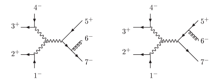
Figure 3: The two Feynman diagrams contributing the seven point amplitude with a triple vector boson self coupling. Wavy lines represent gauge bosons such as the $W$ or $Z$ and curly lines gluons.

A key property of the vector boson currents is that they may be coupled to off-shell electroweak gauge bosons. For example, consider the amplitude containing the non-abelian triple vector boson self coupling (i.e. the $ZW^{+}W^{-}$ coupling), $A_{7}^{{\rm NA}}(1^{-}_{{e^{-}}},2^{+}_{e^{+}},3^{+}_{\mu^{-}},4^{-}_{\mu^{+}},5_{q}^{+},6^{-},7_{\overline{\kern-0.7ptq\kern-0.7pt}}^{-})$, depicted in terms of Feynman diagrams in fig. 3. Up to relabelings and a parity reflection, it corresponds to the amplitude in eq. (2.23) of ref. DKS . As explained in that reference, the sum over these two diagrams is gauge invariant because its electroweak coupling constant differs from diagrams without a triple vector boson self-interaction and hence do not mix with them.

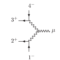
Figure 4: The Feynman diagram for the electroweak vector boson current with a non-abelian triple vector boson self interaction. We may couple this to the QCD vector boson current determined using CSW diagrams.

In our construction this amplitude factorizes into a product of two currents with the connecting propagator. One is the QCD vector boson current described by the NMHV current $J_{\mu}(5_{q}^{+},6^{-},7^{-}_{{\overline{\kern-0.7ptq\kern-0.7pt}}};P_{V})$ obtained by relabeling eq. (28). The electroweak current containing the non-abelian triple vector boson interaction may easily be evaluated by working out the Feynman diagrams shown in fig. 4 in Feynman-’t Hooft or any other gauge. We have verified that combining the two currents reproduces eq. (2.23) of ref. DKS (after accounting for a parity reflection and relabeling). Of course, this example is sufficiently simple so that MHV diagrams are unnecessary. However, with the CSW approach it is straightforward to incorporate larger numbers of quarks and gluons in the vector boson QCD current.

The complete process also includes contributions in which both vector bosons couple directly to the fermion line, given in eqs. (2.8) and (2.22) of ref. DKS . We have verified that a symmetrized double-vector current constructed as described in the previous section reproduces the results of ref. DKS after symmetrization over the two leptonic currents $(3,4)\leftrightarrow(6,5)$.

We have implemented a light-cone version of the Berends–Giele recurrence relations, for the purposes of confirming our extension of CSW diagrams to currents. These are obtained by reshuffling terms from the standard ones (similar to the spirit of ref. LightConeRecursion ). We have used these to check currents computed using the recursive reformulation of the CSW rules, as described in eq. (29). We performed this comparison numerically, for all helicities up to $n=8$ legs (in addition to the leg carrying the vector-boson index). We also checked selected helicities through $n=10$.

VI Conclusions and Outlook

The twistor-inspired computational approach presented by Cachazo, Svrček, and Witten is a novel way of computing tree amplitudes in massless gauge theories, including of course QCD. It relies on a basic set of vertices which are localized in a twistor-space sense. These vertices are particular off-shell continuations of the well-known Parke–Taylor amplitudes. The CSW approach does not address the computation of amplitudes containing both colored and non-colored particles. In the context of the Standard Model, it does not, for example address the question of computing mixed QCD-electroweak processes.

In this paper, we have taken a step in this direction. We have shown how to incorporate an additional vector leg coupling to an arbitrary source into the CSW approach. As we have discussed, multiple symmetrized vector legs ($Z,\gamma^{*}$) follow with a straightforward modification. The propagators and diagrammatic rules are essentially unchanged; it suffices to add new basic vertices with the additional vector leg(s). (Unlike the CSW construction, these vertices do include a two-point vertex.) In our explicit examples, we have focused on coupling one off-shell electroweak vector boson to a single quark pair and any number of gluons. The structure of the CSW construction implies that adding additional quark pairs should be straightforward. We expect that a similar approach can be used to construct multi-$W$s currents, and that ideas presented in this paper also generalize to currents for colored particles. These topics will be elaborated on elsewhere.

To date, no-one has given a complete first-principles proof of the CSW construction. Nonetheless, there is very strong evidence in its favor. As pointed out in the original paper CSW , a CSW computation automatically has the correct collinear and multiparticle-factorization limits. In addition, extensive numerical checks against Berends–Giele recurrence relations (which were derived from first principles) through relatively high multiplicity leave little room for doubt.

The factorization arguments also apply to the currents presented in this paper. We have implemented a light-cone version of the Berends–Giele recurrence relations BGKGluon , and have shown complete agreement between currents computed using them, and currents computed using a recursive MHVRecursive reformulation of the CSW rules. We performed these comparisons numerically, for up to ten legs (in addition to the leg carrying the vector-boson index). Photon amplitudes can be derived from the currents (by contracting with a polarization vector, and taking the on-shell limit), and we have shown that these expressions reproduce the corresponding amplitudes as obtained directly from the CSW rules, after adjusting the color factors to reflect the abelian nature of the photon.

The currents we have constructed can be used directly in the computation of processes producing electroweak vector bosons. We are optimistic that further phenomenologically useful extensions of the CSW approach will be possible.

References

- (1) F. A. Berends and W. T. Giele, Nucl. Phys. B306:759 (1988).
-
(2)
F. Caravaglios and M. Moretti,
Phys. Lett. B 358, 332 (1995)
[hep-ph/9507237];
P. Draggiotis, R. H. P. Kleiss and C. G. Papadopoulos, Phys. Lett. B 439, 157 (1998) [hep-ph/9807207];
F. Caravaglios, M. L. Mangano, M. Moretti and R. Pittau, Nucl. Phys. B539:215 (1999) [hep-ph/9807570]. - (3) T. Stelzer and W. F. Long, Comput. Phys. Commun. 81:357 (1994) [hep-ph/9401258].
- (4) F. Cachazo, P. Svrček and E. Witten, hep-th/0403047.
- (5) E. Witten, hep-th/0312171.
- (6) V. P. Nair, Phys. Lett. B214:215 (1988).
- (7) N. Berkovits, Phys. Rev. Lett. 93:011601 (2004) [hep-th/0402045].
- (8) N. Berkovits and L. Motl, JHEP 0404:056 (2004) [hep-th/0403187].
- (9) A. Neitzke and C. Vafa, hep-th/0402128.
- (10) W. Siegel, hep-th/0404255.
- (11) I. Bena, Z. Bern and D. A. Kosower, hep-th/0406133.
- (12) S. Gukov, L. Motl and A. Neitzke, hep-th/0404085.
-
(13)
F. Cachazo, P. Svrček and E. Witten,
hep-th/0406177;
A. Brandhuber, B. Spence and G. Travaglini, hep-th/0407214;
F. Cachazo, P. Svrček and E. Witten, hep-th/0409245;
I. Bena, Z. Bern, D. A. Kosower and R. Roiban, hep-th/0410054;
F. Cachazo, hep-th/0410077;
R. Britto, F. Cachazo and B. Feng, hep-th/0410179; hep-th/0411107; hep-th/0412103
J. Bedford, A. Brandhuber, B. Spence and G. Travaglini, hep-th/0410280; hep-th/0412108;
C. Quigley and M. Rozali, hep-th/0410278;
Z. Bern, V. Del Duca, L. J. Dixon and D. A. Kosower, hep-th/0410224;
S. J. Bidder, N. E. J. Bjerrum-Bohr, L. J. Dixon and D. C. Dunbar, hep-th/0410296;
S. J. Bidder, N. E. J. Bjerrum-Bohr, D. C. Dunbar and W. B. Perkins, hep-th/0412023. - (14) N. Berkovits and E. Witten, hep-th/0406051.
- (15) S. J. Parke and T. R. Taylor, Phys. Rev. Lett. 56:2459 (1986).
-
(16)
G. Georgiou and V. V. Khoze,
hep-th/0404072;
J. B. Wu and C. J. Zhu, JHEP 0409:063 (2004) [hep-th/0406146];
G. Georgiou, E. W. N. Glover and V. V. Khoze, JHEP 0407:048 (2004) [hep-th/0407027]. - (17) D. A. Kosower, hep-th/0406175.
-
(18)
R. Roiban, M. Spradlin and A. Volovich,
JHEP 0404:012 (2004) [hep-th/0402016];
R. Roiban and A. Volovich, hep-th/0402121. -
(19)
C. J. Zhu,
JHEP 0404:032 (2004)
[hep-th/0403115];
J. B. Wu and C. J. Zhu, JHEP 0407:032 (2004) [hep-th/0406085]. -
(20)
R. Roiban, M. Spradlin and A. Volovich,
Phys. Rev. D70:026009 (2004)
[hep-th/0403190];
M. Aganagic and C. Vafa, hep-th/0403192;
E. Witten, hep-th/0403199. - (21) L. J. Dixon, E. W. N. Glover and V. V. Khoze, hep-th/0411092.
- (22) F. A. Berends, W. T. Giele and H. Kuijf, Nucl. Phys. B321:39 (1989).
- (23) D. A. Kosower, Nucl. Phys. B335:23 (1990).
-
(24)
J. E. Paton and H. M. Chan,
Nucl. Phys. B10:516 (1969);
P. Cvitanovic, P. G. Lauwers and P. N. Scharbach, Nucl. Phys. B186:165 (1981);
F. A. Berends and W. Giele, Nucl. Phys. B294:700 (1987);
D. Kosower, B. H. Lee and V. P. Nair, Phys. Lett. B201:85 (1988);
M. L. Mangano, S. J. Parke and Z. Xu, Nucl. Phys. B298:653 (1988);
Z. Bern and D. A. Kosower, Nucl. Phys. B362:389 (1991);
V. Del Duca, L. J. Dixon and F. Maltoni, Nucl. Phys.B:571, 51 (2000) [hep-ph/9910563]. -
(25)
M. L. Mangano and S. J. Parke,
Phys. Rept. 200:301 (1991);
L. J. Dixon, in QCD & Beyond: Proceedings of TASI ’95, ed. D. E. Soper (World Scientific, 1996) [hep-ph/9601359]. - (26) L. J. Dixon, Z. Kunszt and A. Signer, Nucl. Phys. B531:3 (1998) [hep-ph/9803250].
- (27) Z. Bern, L. J. Dixon and D. A. Kosower, Nucl. Phys. B437:259 (1995) [hep-ph/9409393].
-
(28)
P. De Causmaecker, R. Gastmans, W. Troost and T. T. Wu,
Phys. Lett. B 105, 215 (1981).
F. A. Berends, R. Kleiss, P. De Causmaecker, R. Gastmans,
W. Troost and T. T. Wu,
Nucl. Phys. B206:61 (1982);
P. De Causmaecker, R. Gastmans, W. Troost and T. T. Wu, Nucl. Phys. B206:53 (1982);
J. F. Gunion and Z. Kunszt, Phys. Lett. B161:333 (1985). - (29) Z. Xu, D. H. Zhang and L. Chang, preprint TUTP-84/3-TSINGHUA, unpublished; Nucl. Phys. B 291, 392 (1987).
-
(30)
M. T. Grisaru, H. N. Pendleton and P. van Nieuwenhuizen,
Phys. Rev. D15:996 (1977);
M. T. Grisaru and H. N. Pendleton, Nucl. Phys. B124:81 (1977);
S. J. Parke and T. R. Taylor, Phys. Lett. B157:81 (1985) [Erratum-ibid. B174:465 (1986)];
Z. Kunszt, Nucl. Phys. B271:333 (1986);
Z. Kunszt, A. Signer and Z. Trocsanyi, Nucl. Phys. B411:397 (1994) [hep-ph/9305239]. - (31) F. A. Berends, W. T. Giele and H. Kuijf, Nucl. Phys. 333:120 (1990).