Connection between Second Class Currents and the $\Delta N\gamma$ Form Factors $G_{M}^{\ast}(q^{2})$ and $G_{E}^{\ast}(q^{2})$

Abstract

An interesting connection between the nucleon weak axial-vector second class current form factor $g_{T}(q^{2})$ present in the matrix element $\left\langle{p}\right|A_{\pi^{+}}^{\mu}\left|{n}\right\rangle$ and the $\Delta N\gamma$ form factors $G_{M}^{\ast}(q^{2})$ and $G_{E}^{\ast}(q^{2})$ is derived. Using a nonperturbative, relativistic sum rule approach in the infinite momentum frame, $G_{M}^{\ast}(q^{2})$ and $G_{E}^{\ast}(q^{2})$ are calculated in terms of $g_{T}(q^{2})$ and the well-known nucleon isovector Sachs form factor $G_{M}^{V}$ as input with no additional model parameters. Reasonable agreement with the data for $G_{M}^{\ast}(q^{2})$ may be achieved with a non-zero $g_{T}(q^{2})$ too large to be accommodated in the Standard Model. We surmise that it is plausible that second class current-associated pion cloud effects are playing a significant role in pion electroproduction processes and perhaps must be taken into account in those methodologies which utilize effective Lagrangians.

The study of the nucleon weak axial-vector second class current (SCC)weinberg form factor $g_{T}(q^{2})$ present in the matrix element $\left\langle{p}\right|A_{\pi^{+}}^{\mu}\left|{n}\right\rangle$ and the $\Delta N\gamma$ form factors $G_{M}^{\ast}(q^{2})$ and $G_{E}^{\ast}(q^{2})$ has engendered much experimental and theoretical research for several decadesholstein71 ; kubodera ; monsay ; jonesscadron ; ahrens88 ; stoler93 ; shiomi96 ; tminamisono1998 ; wilkinson2000nim ; kminamisono2000 ; gardner2001 ; abele2002 ; kuzminaug2004 . In a perfect world with unbroken $SU_{F}(N)$ flavor symmetry, one expects that $G_{E}^{\ast}(q^{2})=0$ and that $G_{M}^{\ast}(q^{2})$ would exhibit the same $q^{2}$ behavior as does the Sachs nucleon form factor $G_{M}$. Instead, one unexpectedly finds that, experimentally, $G_{M}^{\ast}$ decreases faster as a function of $Q^{2}\equiv-q^{2}$ than does $G_{M}$ and furthermore, that not only does the ratio $-G_{E}^{\ast}/G_{M}^{\ast}\neq 0$ but indeed, possesses a complicated behavior as a function of $Q^{2}$. In this Letter, we suggest that the inclusion of SCC effects normally neglected in most experimental and theoretical studies in general and in pion photoproduction and electroproduction processes in particular, may aid in our understanding of the basic underlying connecting physics principles responsible for such processes.

We begin by using a nonperturbative, relativistic sum rule approach in the infinite momentum frame where $G_{M}^{\ast}(q^{2})$ and $G_{E}^{\ast}(q^{2})$ are calculated in terms of $g_{T}(q^{2})$ and the well-known nucleon isovector Sachs form factor $G_{M}^{V}$ as input with no additional model parametersmiltnpasub2003 . With regard to shape and data, reasonable agreement for $G_{M}^{\ast}(q^{2})$ may be achieved with a non-zero $g_{T}(q^{2})$ probably too large to be accommodated in the Standard Model (SM). We surmise that it is plausible that SCC-associated pion cloud effects are playing a significant role in pion photoproduction and electroproduction processes and perhaps must be taken into account in those methodologies which utilize effective Lagrangians.

The most general form for the matrix element of the weak current between the proton and the neutron is given by

$$(2\pi)^{3}\sqrt{\frac{E_{p_{1}}E_{p_{2}}}{mm_{n}}}\left\langle P(p_{2})\right|A_{\pi^{+}}^{\mu}(0)\left|N(p_{1})\right\rangle$$ (1)

$$= \bar{u}_{P}(p_{2})\left[\{g_{A}({\tilde{q}}^{2})\gamma^{\mu}+ig_{T}({\tilde{q}}^{2})\sigma^{\mu\nu}{\tilde{q}}_{\nu}+ig_{P}({\tilde{q}}^{2}){\tilde{q}}^{\mu}\}\gamma_{5}\right]u_{N}(p_{1}).$$

The 4-momentum transfer ${\tilde{q}}^{2}=p_{1}-p_{2}$. $g_{A}$, $g_{T}$, and $g_{P}$ are the axial-vector, induced pseudotensor, and induced pseudoscalar form factors respectively. With respect to transformations under G-parity, $g_{A}$ and $g_{P}$ are represented by first-class currents (FCC) while $g_{T}$ is represented by SCC. In the SM, a non-zero $g_{T}$ can only arise due to quark mass and charge differences and thus the ratio $g_{T}/g_{A}$is thought to be very small or identically zero. In Ref.miltnpasub2003 —assuming no SCC effects—the $\Delta N\gamma$ transition form factors $G_{M}^{\ast}(q^{2})$ and $G_{E}^{\ast}(q^{2})$ were calculated in terms of well-known nucleon isovector Sachs form factor parametrized by $G_{M}^{V}({\tilde{q}}^{2})=\frac{1}{2}(\mu_{p}-\mu_{n})G_{\mbox{dipole}}({\tilde{q}}^{2})$, with $G_{\mbox{dipole}}({\tilde{q}}^{2})\equiv[1-{\tilde{q}}^{2}/0.71\ GeV^{2}/c^{2}]^{-2}$, where $\mu_{p}$ and $\mu_{n}$ are the proton and neutron magnetic moments respectively. On the other hand, if one now allows for SCC effects, one obtains:

$$G_{M}^{\ast}(q^{2}) = \left(3c_{2}(q^{2})G_{M}^{V}({\tilde{q}}^{2}_{+})+c_{1}(q^{2})c_{3}(q^{2})\sqrt{{\tilde{Q}}^{+}_{+}{\tilde{Q}}^{-}_{-}}G_{M}^{V}({\tilde{q}}^{2}_{-})\right)/\left((3+c_{1}(q^{2}))\sqrt{{\tilde{Q}}^{+}_{+}}\right),$$ (2)

$$G_{E}^{\ast}(q^{2}) = \left(c_{2}(q^{2})G_{M}^{V}({\tilde{q}}^{2}_{+})-c_{3}(q^{2})\sqrt{{\tilde{Q}}^{+}_{+}{\tilde{Q}}^{-}_{-}}G_{M}^{V}({\tilde{q}}^{2}_{-})\right)/\left((3+c_{1}(q^{2}))\sqrt{{\tilde{Q}}^{+}_{+}}\right),$$ (3)

$$c_{1}(q^{2}) = \frac{m^{*}(4m-m^{*})+m^{2}-q^{2}}{(m^{*2}+m^{2}-q^{2})},$$ (4)

$$c_{2}(q^{2}) = \frac{5\sqrt{3}}{3}\left[-\left(\frac{m^{*}m}{m^{*}+m}\right)\left(\frac{{\tilde{Q}}^{+}_{+}\sqrt{{\tilde{Q}}^{-}_{+}}}{(m^{*2}+m^{2}-q^{2})G_{M}^{V}({\tilde{q}}^{2}_{+})}\right)\left(\frac{g_{T}({\tilde{q}}^{2}_{+})}{g_{A}(0)\sqrt{4\pi\alpha}}\right)\right.$$

$$+ \left.\frac{2m^{*}m^{2}\sqrt{Q^{+}}}{(m^{*}+m)(m^{*2}+m^{2}-q^{2})}\right],$$

$$c_{3}(q^{2}) = \frac{m}{(m^{*}+m)\sqrt{{\tilde{Q}}^{-}_{+}}},$$ (6)

where $\alpha\equiv$ fine-structure constant, $q\equiv p^{\ast}-p$, $p^{\ast}=(p^{\ast 0},\vec{t})$ and $p=(p^{0},\vec{s})$ are the four-momenta of the $\Delta^{+}$ and nucleon respectively, $m^{\ast}=\Delta^{+}$ mass, $m=$ proton mass $\approx$ neutron mass $=m_{n}$, $\widetilde{q}=\widetilde{p}^{\ast}-\widetilde{p}$, $p_{1}=\widetilde{p}^{\ast}=(\widetilde{p}^{\ast 0},\vec{t})$ and $p_{2}=\widetilde{p}=(\widetilde{p}^{0},\vec{s})$, $Q^{\pm}\equiv(m^{\ast}\pm m)^{2}-q^{2}$,${\tilde{q}}^{2}_{\pm}=[(m^{\ast 2}+m^{2})q^{2}+(m^{\ast 2}-m^{2})(\pm\sqrt{Q^{+}Q^{-}}-(m^{\ast 2}-m^{2}))]/(2m^{\ast 2})$, ${\tilde{Q}}^{+}_{\pm}\equiv 4m^{2}-{\tilde{q}}^{2}_{\pm}$, and ${\tilde{Q}}^{-}_{\pm}\equiv-{\tilde{q}}^{2}_{\pm}$. Note that ${\tilde{q}}^{2}_{+}(q^{2}=0)=0$ and also that $g_{P}$ does not contribute to $G_{M}^{\ast}$ and $G_{E}^{\ast}$ in Eqs.(2) and (3). While very little is known about $g_{T}$, it is traditional to model $g_{T}$ as a dipole similar to $g_{A}$ and $G_{M}$: $g_{T}({\tilde{q}}^{2}_{+}))=g_{T}(0)[1-{\tilde{q}}^{2}_{+}/m_{T}^{2}]^{-2}$, where $m_{T}$ is a “pseudotensor mass” analogous to the axial-vector mass $m_{A}\approx 1.2\,GeV/c^{2}$. However, we note, that at present, no theoretical justification for a specific form of $g_{T}$ is known. Indeed, we find that an exponential form such as $g_{T}({\tilde{q}}^{2}_{+}))=g_{T}(0)[exp({\tilde{q}}^{2}_{+}/m_{T}^{2})]$ may also suffice. We also note that $G_{M}^{\ast}(q^{2})$ as defined above is related to another widely used phenomenological form factor $G_{M}^{\ast Ash}(q^{2})$ ash by $G_{M}^{\ast}(q^{2})=G_{M}^{\ast Ash}(q^{2})\sqrt{1-q^{2}/(m^{\ast}+m)^{2}}$ jonesscadron .

From Eqs. (2–6) and given a specific form for $g_{T}$, one may calculate $G_{M}^{\ast}$ and $G_{E}^{\ast}$. In Fig. 1, we present our results for $G_{M}^{\ast Ash}(Q^{2})$ normalized relative to $3\,G_{\mbox{dipole}}(Q^{2})$ along with experimental data. In Fig. 2, we present our results for $G_{E}^{\ast}(Q^{2})$ in terms of the ratio $R_{EM}\equiv-G_{E}^{\ast}/G_{M}^{\ast}$. As is evident, an adequate fit may be achieved by assuming a non-zero $g_{T}$. Interestingly, an exponential form for $g_{T}$ suffices as well as a dipole form when one considers $R_{EM}$ and its behavior in the region $0\leq Q^{2}\lesssim 1\;(GeV/c)^{2}$.

In addition to demonstrating the faster than dipole decrease in $G_{M}^{\ast}$ as a function of $Q^{2}$—in agreement with experiment—and the change in sign of $R_{EM}$ as $Q^{2}$ increases—as indicated by experiment—the curves in Fig. 1 and Fig. 2 suggest that the small (close to the real photon point) $Q^{2}$ behavior of both $G_{M}^{\ast}$ and $G_{E}^{\ast}$ may be much more complex than one may have perhaps anticipated and indeed may signal the presence of a SCC contribution to basic pion electroproduction processes. If this is indeed the case, a possible explanation could be pion cloud effects associated with the matrix element $\left\langle{p}\right|A_{\pi^{0}}^{\mu}\left|{p}\right\rangle\propto\left\langle{p}\right|A_{\pi^{+}}^{\mu}\left|{n}\right\rangle$ which may have to be explicitly included in dynamical approaches to pion photoproduction and electroproduction.

The author is grateful to Professor Paul Stoler for providing data used in this work and for very useful and provocative communications.

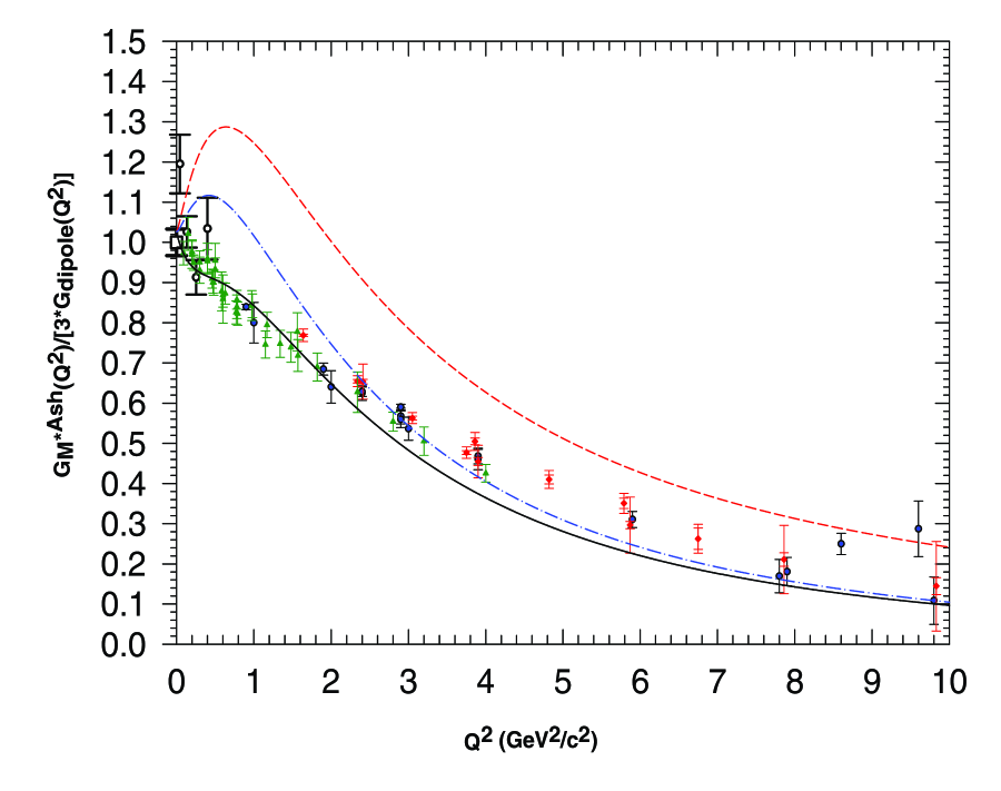
Figure 1: $G_{M}^{\ast Ash}(Q^{2})$ normalized to $3\,G_{\mbox{dipole}}(Q^{2})$. Theoretically calculated Dashed curve with $g_{T}=0$ as discussed in the text with $G_{M}^{\ast}(0)/3\,G_{\mbox{dipole}}(0)=1.03$; The Solid curve is a $g_{T}$ dipole fit to the JLAB $G_{M}^{\ast}$ data of Ref. kamalov1 where $g_{T}(0)/g_{A}(0)=1.169\;c^{2}/GeV$, $m_{T}=0.534\;GeV/c^{2}$ is obtained; The Dot-Dashed curve is a $g_{T}$ exponential fit to the JLAB $G_{M}^{\ast}$ data of Ref. kamalov1 where $g_{T}(0)/g_{A}(0)=0.663\;c^{2}/GeV$, $m_{T}=0.630\;GeV/c^{2}$ is obtained; Open Square data point is from Ref. ash ) where $G_{M}^{\ast}(0)=3.00\pm.01$; Diamond denoted data is from Ref. stuart ; Down-Triangle denoted data is from Ref. stein ; Square denoted data is from Ref. stoler93 ; Open-Circle denoted data is from Ref. mistretta ; Up-Triangle denoted data is from Ref. kamalov1 .

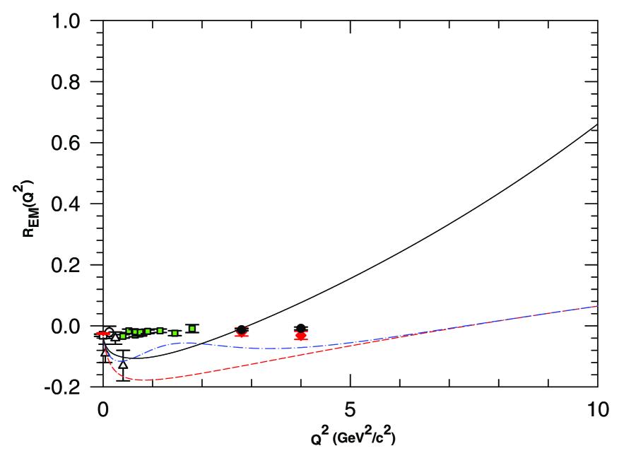
Figure 2: Electromagnetic ratio $R_{EM}(Q^{2})$. Theoretically calculated Dashed curve with $g_{T}=0$ as discussed in the text with $R_{EM}(0)=-0.038$; The Solid curve utilizes the results of the $g_{T}$ dipole fit to the JLAB $G_{M}^{\ast}$ data of Ref. kamalov1 where $g_{T}(0)/g_{A}(0)=1.169\;c^{2}/GeV$, $m_{T}=0.534\;GeV/c^{2}$ is obtained; The Dot-Dashed curve utilizes the results of the $g_{T}$ exponential fit to the JLAB $G_{M}^{\ast}$ data of Ref. kamalov1 where $g_{T}(0)/g_{A}(0)=0.663\;c^{2}/GeV$, $m_{T}=0.630\;GeV/c^{2}$ is obtained; Open Square data point is from Ref. Blanpied ; Diamond denoted data is from Ref. frolov ; Circle denoted data is from Ref. kamalov1 ; Square denoted data is from Ref. joo ; Down-Triangle data point is from Ref. beckprc61 ; Open-Circle data point is from Ref. mertz ; Up-Triangle denoted data is from Ref. mistretta .

References

(1) S. Weinberg, Phys. Rev. 112, 1375 (1958).
(2) B. Holstein, Phys. Rev. C4, 764 (1971).
(3) K. Kubodera, J. Delorme, and M. Rho, , Phys. Rev. Lett. 38, 321 (1977).
(4) E. H. Monsay, Phys. Rev. D16, 609 (1977).
(5) H. F. Jones and M. Scadron, Ann. Phys. 81, 1 (1973).
(6) L. A. Ahrens, et al., Phys. Lett. 202B, 284 (1988).
(7) P. Stoler, Phys. Rep. 226, 103 (1993).
(8) H. Shiomi, Nucl. Phys. A603, 281 (1996).
(9) T. Minamisono et al., Phys. Rev. Lett. 80, 4132 (1998).
(10) D. H. Wilkinson, Nucl. Instrum. Meth. A455,656 (2000).
(11) K. Minamisono et al., Nucl. Phys. A663, 951 (2000).
(12) S. Gardner and C. Zhang, Phys. Rev. Lett. 86, 5666 (2001).
(13) H. Abele, et al., Phys. Rev. Lett. 88, 211801 (2001).
(14) K. S. Kuzmin, V. V. Lyubushkin, V. A. Naumov, hep-ph/0408107 (2004).
(15) M. D. Slaughter, Nuc. Phys. A740, 383 (2004).
(16) W. W. Ash et al., Phys. Lett. 24B, 165 (1967).
(17) S. S. Kamalov et al., Phys. Rev. C64,
032201(R) (2001); S. S. Kamalov et al., Nuc. Phys. A684, 321c (2001).
(18) L. M. Stuart et al., Phys. Rev. D58, 032003 (1998).
(19) S. Stein et al., Phys. Rev. D12, 1884 (1975).
(20) C. Mistretta et al., Phys. Rev. 184, 1487 (1969).
(21) R. Beck et al., Phys. Rev. C61, 035204 (2000).
(22) G. Blanpied et al., Phys. Rev. C64, 025203 (2001).
(23) V. V. Frolov et al., Phys. Rev. Lett. 82, 45 (1999).
(24) K. Joo et al., Phys. Rev. Lett. 88, 122001-1 (2002).
(25) C. Mertz et al., Phys. Rev. Lett. 86, 2963 (2001).