TUHEP-TH-03142

Distinguishing technicolor models via $t\bar{t}$ productions at polarized photon colliders

Abstract

We study top quark pair productions at a polarized photon collider from an $e^{+}e^{-}$ linear collider (LC) in various improved technicolor model, namely, the one-family walking technicolor model, the top-color-assisted technicolor model, and the top-color-assisted multiscale technicolor model. Recent constraint on the top-pion mass from the precision data of $R_{b}$ is considered. It is shown that, considering only the statistical errors, a polarized photon collider from a 500 GeV LC with an integrated luminosity of 500 fb^-1 is sufficient for distinguishing the three improved technicolor models experimentally.

PACS number(s): 12.60.Nz, 13.40.-f, 14.65.Ha

Although the standard model (SM) has successfully passed the precision electroweak tests, its elecrtoweak symmetry breaking (EWSB) mechanism is still unclear. The Higgs boson has not been found, and the LEP2 bound on the Higgs boson mass is 114.4 GeV PDG . Furthermore, the SM Higgs sector suffers from the well-known problems of triviality and unnaturelness arising from the elementary Higgs field. There have been many new physics models of the EWSB mechanism proposed for avoiding the above problems. An attractive idea of completely avoiding triviality and unnatureness is to abandon the elementary Higgs field(s), such as various kinds of improved technicolor models AT ; TOPCTC ; TOPCMTC , top quark seesaw models seesaw , and certain little Higgs models littleHiggs . In a previous paper ZKYWL , we studied the tests of various improved technicolor models via top quark pair productions at high energy photon colliders. Since the pseudo Goldstone bosons (PGBs) coupling to the top quark in different improved technicolor models are quite different, we showed that different improved technicolor models can be distinguished experimentally through top quark pair productions at an unpolarized photon collider built from a $\sqrt{s}=1.5$ TeV $e^{+}e^{-}$ linear collider (LC) ZKYWL . In this paper, we study the same processes at polarized photon colliders, and take into account the recent bound on the top-pion mass from the precision data of $R_{b}$ YKWL . We shall see that, considering only statistical uncertainties, a polarized photon collider built from a $\sqrt{s}=500$ GeV LC with an integrated luminosity of 500 fb^-1 is sufficient for distinguishing the improved technicolor models.

It has been shown that the polarization of the initial laser beam and the electron beam will significantly affect the photon spectrum at the photon collider Ginzburg . Let $P_{c}$ be the polarization of the initial laser, $\lambda_{e}$ be the polarization of the electron in the first beam, and $\tilde{P}_{c}$ and $\tilde{\lambda}_{e}$ be the corresponding parameters in the second beam, respectively. It is shown in Ref.Ginzburg that the colliding photons will peak in a narrow region near the high energy end ($80\%$ of the electron energy) if $2\lambda_{e}P_{c}=-1$. This improves the monochromatization and enhances the effective energy of the colliding photons at the photon collider. We shall see that this effect leads to the possibility of distinguishing different iomproved technicolor models at a polarized photon collider built from a $\sqrt{s}=500$ GeV LC.

Let $E_{e},~{}\omega_{0},~{}\omega$, and $\sqrt{s}(\sqrt{\hat{s}})$ be the incident elecrton energy, the laser-photon energy, the backscattered photon energy, and the center-of-mass energies of $e^{+}e^{-}$($\gamma\gamma$), respectively. The photon luminosity $dL_{\gamma\gamma}$ is luminosity

$$dL_{\gamma\gamma}=2zdz\int^{x_{max}}_{z^{2}/x_{max}}\frac{dx}{x}F_{\gamma/e}(x)F_{\gamma/e}(z^{2}/x).$$ (1)

with $z=\sqrt{\hat{s}/s}$, and $x_{max}=\omega_{max}/E_{e}$,

$$F_{\gamma/e}(x) = \frac{1}{D(\xi)}\bigg{[}1-x+\frac{1}{1-x}-\frac{4x}{\xi(1-x)}+\frac{4x^{2}}{\xi^{2}(1-x)^{2}}$$

$$-2\lambda_{e}P_{c}\bigg{(}\frac{x}{1-x}-\frac{2x^{2}}{(1-x)^{2}\xi}\bigg{)}(2-x)\bigg{]},$$

and

$$D(\xi)=\bigg{(}1-\frac{4}{\xi}-\frac{8}{\xi^{2}}\bigg{)}\ln(1+\xi)+\frac{1}{2}+\frac{8}{\xi}-\frac{1}{1(1+\xi)^{2}},$$

where $\xi=4E_{e}\omega_{0}/m_{e}^{2}$. In order to avoid the creation of $e^{+}e^{-}$ pairs by the interaction of the incident and backscattered photons, $\xi$ should not be larger than 4.8 Ginzburg . As in Ref.ZKYWL , we take $\xi=4.8$, then $x_{max}\approx 0.83$ and $D(\xi)=1.8$. The formula for the counting rate of $\gamma\gamma\to X$ at a polarized photon collider has been given in Ref.Ginzburg . It is

$$d\dot{N}_{\gamma\gamma\to X} = dL_{\gamma\gamma}(d\sigma+\Lambda d\tau+\zeta_{2}\tilde{\zeta}_{2}d\tau^{a}+\zeta_{2}d\sigma_{20}$$ (2)

$$+\tilde{\zeta}_{2}d\sigma_{02}),$$

where $\zeta_{i}~{}(\tilde{\zeta}_{i}),~{}i=1,2,3$ are Stokes parameters Ginzburg ,

$$\zeta_{2}=\frac{C_{20}}{C_{00}},$$

$$C_{00}=\frac{1}{1-x}+1-x-4r(1-r)$$

$$\hskip 28.45274pt-2\lambda_{e}P_{c}r\xi(2r-1)(2-x)$$

$$C_{20}=2\lambda_{e}r\xi[1+(1-x)(2r-1)^{2}]$$

$$\hskip 28.45274pt-P_{c}(2r-1)(\frac{1}{1-x}+1-x),$$

$$x\equiv\frac{\omega}{E_{e}},~{}~{}~{}~{}~{}~{}r\equiv\frac{x}{\xi(1-x)},$$

$\sigma_{ij},~{}i,j=0,1,2,3~{}$ are cross sections defined in Ref.BGMS , $\Lambda=\langle\zeta_{3}\tilde{\zeta}_{3}-\zeta_{1}\tilde{\zeta}_{1}\rangle$ Ginzburg , and $d\sigma$, $d\tau^{a}$ are Ginzburg

$$d\sigma = \frac{1}{4}(|M_{++}|^{2}+|M_{--}|^{2}+|M_{+-}|^{2}$$

$$+|M_{-+}|^{2})d\Gamma,$$

$$d\tau^{a} = \frac{1}{4}(|M_{++}|^{2}+|M_{--}|^{2}-|M_{+-}|^{2}$$ (3)

$$-|M_{-+}|^{2})d\Gamma,$$

in which the subscripts $+$ and $-$ indicate that the photon helicity is $+1$ and $-1$, respectively, and

$$d\Gamma=\frac{(2\pi)^{4}}{4k\tilde{k}}\delta(k+\tilde{k}-\sum_{f}p_{f})\prod_{f}\frac{d^{3}p_{f}}{(2\pi)^{3}2\epsilon_{f}},$$

where $k,~{}\tilde{k}$ and $p_{f}$ are four momenta of the colliding photons and the $f$-th final state particle, respectively. After averaging over the azimuthal angles, $d\sigma_{20}$ and $d\sigma_{02}$ vanish, and $\Lambda d\tau^{a}$ is negligibly small. So Eq. (2) becomes

$$d\dot{N}_{\gamma\gamma\rightarrow X}=dL_{\gamma\gamma}(d\sigma+\zeta_{2}\tilde{\zeta}_{2}d\tau^{a}).$$ (4)

The corresponding cross section $\sigma(s)$ at an LC with center-of-mass energy $\sqrt{s}$ can be obtained by further integrating Eq. (4) over the parameter $z$ luminosity

$$\sigma(s)=\int^{x_{max}}_{2m_{t}/\sqrt{s}}\frac{d\dot{N}_{\gamma\gamma\to X}}{dz}dz.$$ (5)

For the detection of the final state $t\bar{t}$, we know that the dominant decay mode of the top quark is $t\to W^{+}b$. The $W$ boson will then decay into either two leptons $l^{+}\nu_{l}$ or two quarks $q\bar{q}^{\prime}$. We take the hadronic mode $q\bar{q}^{\prime}$ for detecting the final state signal. The branching ratio of $W\to q\bar{q}^{\prime}$ is $B(W\to q\bar{q}^{\prime})=68\%$ PDG . So the signal contains six jets including two b-quark jets. To separate the six jets, we follow Ref. JLC to impose a cut on the clustering of jets. Let ${\hat{y}}$ be the jet-invariant-masses normalized by the visible energy. The imposed cut is JLC

$${\hat{y}}>{\hat{y}}_{cut}=5\times 10^{-3}.$$ (6)

A possible background is $\gamma\gamma\to W^{+}W^{-}Z$ with $Z\to b\bar{b}$. We know that, at $\sqrt{s}=500$ GeV, the cross section $\sigma(\gamma\gamma\to W^{+}W^{-}Z)$ is about a factor of two smaller than $\sigma(\gamma\gamma\to t\bar{t})$ photoncollider , and the branching ratio of $Z\to b\bar{b}$ is $B(Z\to b\bar{b})=15\%$. So that this background is smaller than the signal by an order of magnitude.

Another possible background is $\gamma\gamma\to W^{+}W^{-}$ in which the hadronization of quarks forms six jets JLC . In $e^{+}e^{-}$ collision, the background cross section $\sigma(e^{+}e^{-}\to W^{+}W^{-})$ is much larger than the signal cross section $\sigma(e^{+}e^{-}\to t\bar{t})$ photoncollider . However, after taking the cut (6), the signal-to-background ratio can be made greater than 10 JLC . At the photon collider with $\sqrt{s}=500$ GeV, the signal cross section $\sigma(\gamma\gamma\to t\bar{t})$ is about the same as $\sigma(e^{+}e^{-}\to t\bar{t})$, while the background cross section $\sigma(\gamma\gamma\to W^{+}W^{-})$ is about a factor of 10 larger than $\sigma(e^{+}e^{-}\to W^{+}W^{-})$ photoncollider . Hence, at the photon collider, the signal-to-background ratio after imposing the cut (6) is about 1. So we have to tag at least one $b$-jet to suppress the background. We know that the $b$-tagging efficiency at LEP and at the Tevatron is around $(50\--60)\%$. We shall take $50\%$ for the $b$-tagging efficiency in the following study.

Our calculation shows that the cut (6) reduces the signal cross section $\sigma(\gamma\gamma\to t\bar{t})$ by a factor of $47\%$ in both the SM and the technicolor models for the parameter range under consideration. To be more realistic, we take into account the fact that the detector cannot detect jets in certain forward and backward zones along the beam line. As a conservative estimate, we take the polar angle (relative to the beam line) of the undetectable zones to be $\theta<20^{\circ}$ and $\theta>160^{\circ}$. So we require all the six jets to be in the detectable region $20^{\circ}<\theta<160^{\circ}$. Practically, $b$-tagging is effective only in the region $30^{\circ}<\theta<150^{\circ}$. So we further require the tagged $b$-jet and/or $\bar{b}$-jet to be in this effective region. There can be two possible cases:

(a) Both $b$ and $\bar{b}$ jets are in the $b$-tagging effective region $30^{\circ}<\theta<150^{\circ}$, while the other four jets are in the detectable region $20^{\circ}<\theta<160^{\circ}$. Our calculation shows that the probability of satisfying this requirement is $58.3\%$. In this case, it is possible to tag both the $b$ and the $\bar{b}$ jets. Now we only need to tag one of them without specifying whether it is $b$ or $\bar{b}$. For each one of them, the probability of not being tagged is $50\%$. So the probability of both of them not being tagged is $25\%$. Therefore our actual $b$-tagging efficiency in this case is $75\%$.

(b) One tagged $b$ (or $\bar{b}$) jet is in the $b$-tagging effective region $30^{\circ}<\theta<150^{\circ}$, and the untagged $\bar{b}$ (or $b$) jet is in the detectable but not $b$-tagging effective region $20^{\circ}<\theta<30^{\circ}$. The other four jets are in the detectable region $20^{\circ}<\theta<160^{\circ}$. Our calculation shows that the probability of satisfying this requirement is $10\%$. In this case the $b$-tagging efficiency is $50\%$.

Taking into account both of these two possible cases and the $W$ decay branchiong ratio $B(W\to q\bar{q}^{\prime})=68\%$, our final detection efficiency is

$$(68\%)^{2}\times 47\%\times(58.3\%\times 75\%+10\%\times 50\%)\approx 10\%.$$ (7)

In recent years, two of the $e^{+}e^{-}$ linear collider projects have been actively pushed. They are the DESY TeV Energy Superconducting Linear Accelerator (TESLA) with the designed luminosity of $3.4\times 10^{34}$ cm^-2sec^-1 TESLA-I corresponding to $\int_{yr}{\cal L}dt=340$ fb^-1, and the KEK Joint Linear Collider (JLC) with the designed luminosity of $(8\--9)\times 10^{33}$ cm^-2sec^-1 JLC corresponding to $\int_{yr}{\cal L}dt=(80\--90)$ fb^-1. As usual, we shall take an integrated luminosity of 500 fb^-1 and the $10\%$ detection efficiency to estimate the numbers of events ($N_{events}$) of $\gamma\gamma\to t\bar{t}$. In this paper, only statistical errors are taken into account.

In the following, we calculate the helicity amplitudes in Eq. (3) for $\gamma\gamma\to t\bar{t}$ in various improved technicolor models. As what we did in Ref.ZKYWL , for avoiding singularities arising from the very forward or very backward scatterings, we take the rapidity and transverse momentum cuts

$$|y|<2.5,~{}~{}~{}~{}~{}~{}~{}~{}p_{T}>20~{}{\rm GeV}$$ (8)

which will also increase the relative corrections.

As in Ref.ZKYWL , we study the PGB contributions to $\gamma\gamma\to t\bar{t}$ in three technicolor models, namely Model A: the one-family walking technicolor model by Appelquist and Terning AT , Model B: the top-color-assisted technicolor model by Hill TOPCTC , and Model C: the top-color-assited multiscale technicolor model by Lane TOPCMTC . The PGBs in these three models are quite different. This is the main reason why the three models can be distinguished. The formulas for the PGB-$t\bar{t}$ couplings in the three models and the production amplitudes are given in Ref.ZKYWL .

Model A:

In Model A, color-singlet PGBs are composed of technileptons, which do not couple to $t\bar{t}$. Thus there is no $s$-channel resonance contribution in this model. The relevant PGBs are the color-octet technipions containing the $SU(2)_{W}$-singlet $\Pi^{0}_{a}$ and the $SU(2)_{W}$-triplet $\Pi^{\alpha}_{a}$. Their masses are in the few hundred GeV range, and their decay constant is $f_{Q}\approx 140$ GeV AT . The coupling of these PGBs to $t(b)$-quark is AT

$$\displaystyle\frac{\sqrt{2}m_{t}}{f_{Q}}\big{(}i\bar{t}\gamma_{5}\frac{\lambda^{a}}{2}t\Pi^{0}_{a}+i\bar{t}\gamma_{5}\frac{\lambda^{a}}{2}t\Pi^{3}_{a}+\frac{1}{\sqrt{2}}\bar{t}(1-\gamma_{5})\frac{\lambda^{a}}{2}b\Pi^{+}_{a}$$

$$\hskip 28.45274pt+\frac{1}{\sqrt{2}}\bar{b}(1+\gamma_{5})\frac{\lambda^{a}}{2}t\Pi^{-}_{a}\big{)}.$$ (9)

Table 1: Technipion corrections to the $\gamma\gamma\to t\bar{t}$ cross section $\Delta\sigma$, the relative correction $\Delta\sigma/\sigma_{0}$, the total cross section $\sigma=\sigma_{0}+\Delta\sigma$, and $N_{events}$ for an integrated luminosity of 500 fb^-1 taking account of the $10\%$ detection efficiency at a 500 GeV $e^{+}e^{-}$ linear colliderfor with $2\lambda_{e}P_{c}=-1$ for various values of $m_{\Pi_{a}}$ in Model A (The SM cross section is $\sigma_{0}=196$ fb).

$m_{\Pi_{a}}$(GeV)	$\Delta\sigma$ (fb)	$\Delta\sigma/\sigma_{0}$ ($\%$)	$\sigma$ (fb)	$N_{events}$
250	-31	-15.8	165	8250
300	-26	-13.3	170	8500
350	-22	-11.2	174	8700
400	-19	-9.7	177	8850
500	-14	-7.1	182	9100

These color-octet PGBs contribute to $\gamma\gamma\to t\bar{t}$ only through radiative corrections which are small. We list, in TABLE I, the obtained $\Pi_{a}$ corrections to the $\gamma\gamma\to t\bar{t}$ cross section $\Delta\sigma$, the relative correction $\Delta\sigma/\sigma_{0}$ ($\sigma_{0}$ stands for the SM cross section), the total cross section $\sigma=\sigma_{0}+\Delta\sigma$, and $N_{events}$ for an integrated luminosity of 500 fb^-1 at a polarized photon collider from a 500 GeV LC with the polarization $2\lambda_{e}P_{c}=-1$ for $m_{\Pi_{a}}$ in the range $250~{}{\rm GeV}<m_{\Pi_{a}}<500~{}{\rm GeV}$ given in Ref. AT . We see that the corrections $\Delta\sigma$ are negative which are mainly from the interference between the PGB-amplitude and the SM-amplitude. The absolute square of the PGB-amplitude is not large in this model. We see from TABLE I that the total cross sections $\sigma$ are much larger than those given in Ref.ZKYWL due to the enhancement of the effective photon energy in the high energy region at the polarized photon collider. We see that $N_{events}$ for an integrated luminosity of 500 fb^-1 taking account of the $10\%$ detection efficiency are $(8\--9)\times 10^{3}$. The corresponding $95\%$ statistical uncertainties are about $2\%$. Comparing with the relative corrections $\Delta\sigma/\sigma_{0}\sim-(7\--16)\%$ listed in TABLE I, we see that the $\Pi_{a}$ correction effect can be clearly detected.

Model B:

Model B contains a technicolor sector and a top-color sector. The technicolor sector only contributes a small portion of the the top quark mass, say $m_{t}^{\prime}=\epsilon m_{t}$ ($\epsilon\ll 1$), while most of the top quark mass is contributed from the top-color sector, say $m_{t}-m_{t}^{\prime}=(1-\epsilon)m_{t}$. The $b\to s\gamma$ experiment requires $\epsilon<0.1$ Balaji . In this paper, we take a typical value $\epsilon=0.08$, i.e., $m_{t}^{\prime}=0.08m_{t}\approx 14$ GeV as an example to do the study.

In the technicolor sector, the coupling of the color-octet technipion to $t(b)$-quark is similar to Eq. (9) but with $m_{t}/f_{Q}$ replaced by $m_{t}^{\prime}/f_{\Pi}$ ZKYWL , i.e.,

$$\displaystyle\frac{\sqrt{2}m_{t}^{\prime}}{f_{\Pi}}\bigg{(}i\bar{t}\gamma_{5}\frac{\lambda^{a}}{2}t\Pi^{0}_{a}+i\bar{t}\gamma_{5}\frac{\lambda^{a}}{2}t\Pi^{3}_{a}+\frac{1}{\sqrt{2}}\bar{t}(1-\gamma_{5})\frac{\lambda^{a}}{2}b\Pi^{+}_{a}$$

$$\hskip 22.76228pt+\frac{1}{\sqrt{2}}\bar{b}(1+\gamma_{5})\frac{\lambda^{a}}{2}t\Pi^{-}_{a}\bigg{)}.$$ (10)

In addition to the color-octet technipions, there are also color-singlet technipions $\Pi^{0}$ and $\Pi^{3}$, composed of techniquarks, with the decay constant $F_{\Pi}\approx 120$ GeV, and masses in the few hundred GeV range. The coupling of these color-singlet PGBs to $t(b)$-quarks is ZKYWL

$$\displaystyle\frac{c_{t}m^{\prime}_{t}}{\sqrt{2}f_{\Pi}}\bigg{(}i\bar{t}\gamma_{5}t\Pi^{0}+i\bar{t}\gamma_{5}t\Pi^{3}+\frac{1}{\sqrt{2}}\bar{t}(1-\gamma_{5})b\Pi^{+}$$

$$\hskip 22.76228pt+\frac{1}{\sqrt{2}}\bar{b}(1+\gamma_{5})t\Pi^{-}\bigg{)},~{}~{}~{}~{}~{}~{}c_{t}=1/\sqrt{6}.$$ (11)

In the top-color sector, there are color-singlet top-pions $\Pi_{t}^{0}$ and $\Pi_{t}^{\pm}$ with the decay constant $F_{\Pi_{t}}\approx 50$ GeV. The coupling of top-pions to $t(b)$-quark is ZKYWL

$$\frac{m_{t}-m_{t}^{\prime}}{\sqrt{2}f_{\Pi_{t}}}\bigg{(}i\bar{t}\gamma_{5}t\Pi_{t}^{0}+\frac{1}{\sqrt{2}}\bar{t}(1-\gamma_{5})b\Pi_{t}^{+}$$

$$\hskip 22.76228pt+\frac{1}{\sqrt{2}}\bar{b}(1+\gamma_{5})t\Pi_{t}^{-}\bigg{)}.$$ (12)

Recently, it has been pointed out that the LEP precision data of $R_{b}$ gives important constraint on the top-pion mass YKWL . With $\epsilon=0.08$, the $2\sigma$ bound from $R_{b}$ on the top-pion mass in this model is roughly $300~{}{\rm GeV}\leq m_{\Pi_{t}}\leq 900$ GeV YKWL . The naturalness of the model favors lower values of $m_{\Pi_{t}}$. So we take $300~{}{\rm GeV}\leq m_{\Pi_{t}}\leq 500~{}{\rm GeV}$ in this study. In Ref.ZKYWL , $m_{\Pi_{t}}$ was taken to be in the range of $180\--300$ GeV according to the original paper, Ref.TOPCTC . Such a range is below the recent lower bound. We shall see that the updated heavier $\Pi_{t}$ will make the situation quite different at the polarized photon collider from the 500 GeV LC.

The color-singlet PGBs $\Pi^{0}$, $\Pi^{3}$ and $\Pi_{t}^{0}$ couple to the initial state photons through triangle fermion loops (techniquark loops and top quark loops), so they can contribute $s$-channel resonances in $\gamma\gamma\to t\bar{t}$. The triangle fermion loops are enhanced by the anomaly, so that the $s$-channel resonance contributions can be of the order of tree level contributions. These $s$-channel resonance contributions are dominant in Model B and Model C. If the PGB mass is greater than $2m_{t}$, it can decay into $t\bar{t}$. The decay rate is determined by the PGB-$t-\bar{t}$ coupling strengths given in Eqs. (11) and (12). Since $m_{t}-m_{t}^{\prime}/f_{\Pi_{t}}$ in Eq. (12) is large, the width of $\Pi_{t}^{0}$ will be large if its mass is greater than $2m_{t}$. In this case, the $s$-channel resonance effect from $\Pi^{0}_{t}$ is not so significant. On the other hand, $m_{t}^{\prime}/f_{\pi}$ in Eq. (11) is small, so that the resonance effects from $\Pi^{0}$ and $\Pi^{3}$ are significant even their masses are greater than $2m_{t}$. The width of $\Pi^{3}$ is very small which is hard to detect experimentally ZKYWL . So we concentrate on examining the $s$-channel resonance effect of $\Pi^{0}$, and simply take a typical mass of $m_{\Pi^{3}}=300$ GeV for $\Pi^{3}$.

Table 2: Technipion and top-pion corrections to the $\gamma\gamma\to t\bar{t}$ cross section $\Delta\sigma$, the relative correction $\Delta\sigma/\sigma_{0}$, the total cross section $\sigma=\sigma_{0}+\Delta\sigma$, and $N_{events}$ for an integrated luminosity of 500 fb^-1 taking account of the $10\%$ detection efficiency at a 500 GeV $e^{+}e^{-}$ linear colliderfor with $2\lambda_{e}P_{c}=-1$ for $m_{t}^{\prime}$=14 GeV, $m_{\Pi^{3}}=300$ GeV, and various values of $m_{\Pi_{t}^{0}}$ and $m_{\Pi^{0}}$ in Model B (The SM cross section is $\sigma_{0}=196$ fb).

$m_{\Pi_{t}}=300$GeV
$m_{\Pi^{0}}$	$\Delta\sigma$ (fb)	$\Delta\sigma/\sigma_{0}$ ($\%$)	$\sigma$ (fb)	$N_{events}$
300	-86.2	-44.0	110	5500
400	-47.2	-24.1	149	7450
500	-87.4	-44.6	109	5450
$m_{\Pi_{t}}=400$GeV
$m_{\Pi^{0}}$	$\Delta\sigma$ (fb)	$\Delta\sigma/\sigma_{0}$ ($\%$)	$\sigma$ (fb)	$N_{events}$
300	112	57.1	308	15400
400	158.3	80.8	354	17700
500	115	58.7	311	15550

The obtained $\Delta\sigma$, $~{}\Delta\sigma/\sigma_{0}$, $~{}\sigma$, and $N_{events}$ for an intefrated lumionosity of 500 fb^-1 taking account of the $10\%$ detection efficiency for $m_{\Pi_{t}^{0}}$=300 and 400 GeV, and $m_{\Pi^{0}}$=300,  400, and  500 GeV in this model are listed in TABLE II. We see that, in the case of $m_{\Pi_{t}^{0}}$=300 GeV, $\Delta\sigma$ is more negative than in Model A because there is $s$-channel $\Pi_{t}^{0}$ and $\Pi^{0}$ resonance contributions in addition to the radiative corrections, and the $s$-channel resonance contributions are mainly from the interferences between the PGB-amplitudes and the SM-amplitude. In the case of $m_{\Pi_{t}^{0}}$=400 GeV, $\Delta\sigma$ becomes positive. This is because that the absolute squares of the $\Pi_{t}$ and $\Pi^{0}$ resonance amplitudes are large in this case due to the enhancement of the photon spectral luminosity in the region around 400 GeV ($80\%$ 0f the $e^{+}e^{-}$ energy) in the case of $2\lambda_{e}P_{c}=-1$ at the polarized photon collider Ginzburg .

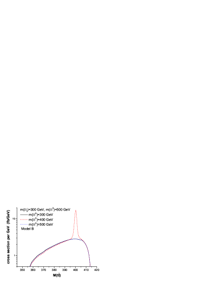
Figure 1: $t\bar{t}$ invariant mass distribution in Model B for $m_{\Pi_{t}}$=300 GeV and $m_{\Pi}$=300, 400, and 500 GeV.

To have an insight of the detailed situation, we plot the $t\bar{t}$ invariant mass distributions in Fig. 1 and Fig. 2 for the six sets of parameters in TABLE II. Fig. 1 shows the invariant mass distributions for $m_{\Pi_{t}}$=300 GeV, $m_{\Pi}$=300, 400, and 500 GeV. We see that all curves are enhanced in the region around 400 GeV which is just the effect of the photon spectral luminosity. In the $m_{\Pi^{0}}=400$ GeV distribution, we see a clear peak at 400 GeV. In the $m_{\Pi^{0}}=300$ and 500 GeV distributions no clear peaks can be seen. This is because that the probability of the center-of-mass energy of the two colliding photons being 300 or 500 GeV is very small as can be seen from the photon spectral luminosity Ginzburg . We cannot see the top-pion resonance since the width of top-pion is much larger. Fig. 2 shows the invariant mass distributions for $m_{\Pi_{t}}$=400 GeV. The behaviors are similar but the enhancement around 400 GeV is stronger due to the $s$-channel contribution of the $m_{\Pi_{t}}=400$ GeV top-pion.

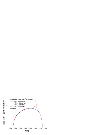
Figure 2: $t\bar{t}$ invariant mass distribution in Model B for $m_{\Pi_{t}}$=400 GeV and $m_{\Pi}$=300, 400, and 500 GeV.

In the case of $m_{\Pi_{t}}$=300 GeV, $N_{events}$ is $(5.4\--7.5)\times 10^{3}$ (cf. TABLE II). The $95\%$ C.L. statistical uncertainties are thus $(2\--3)\%$. Comparing with the relative corrections $\Delta\sigma/\sigma_{0}=(24\--45)\%$ in TABLE II, we see that these correction effects can be very clearly detected. For distinguishing Model B from Model A, we see that the relative difference between the total cross sections in Model A and Model B is $[\sigma(A)-\sigma(B)]/\sigma(A)=(15\--40)\%$, so that these two models can be very clearly distinguished.

In the case of $m_{\Pi_{t}}$=400 GeV, $N_{events}$ is $(1.5\--1.7)\times 10^{4}$. The corresponding $95\%$ C.L. statistical uncertainties are $(1.5\--1.6)\%$. Now the relative corrections are $\Delta\sigma/\sigma_{0}=(57\--81)\%$ in TABLE II, so that these correction effects can be very clearly detected. The relative difference between the total cross sections in Model A and Model B is now $[\sigma(A)-\sigma(B)]/\sigma(A)=-(71\--100)\%$, thus these two models can be very clearly distinguished.

Model C:

Model C is similar to Model B, but the decay constant of the color-singlet technipions is $f_{\Pi}=40$ GeV rather than $f_{\Pi}\approx 120$ GeV TOPCMTC . Moreover, the coupling constant $c_{t}$ in Eq. (11) and the $\Pi^{0}$-$\gamma$-$\gamma$ coupling are also different from those in Model B TOPCMTC ; ZKYWL . The smallness of $f_{\Pi}$ makes the coupling constants $m_{t}^{\prime}/f_{\Pi}$ in Eqs. (10) and (11) larger than those in Model B by a factor of 3. These changes enhance the the $s$-channel $\Pi^{0}$ resonance effect in Model C significantly. Furthermore, the $2\sigma$ $R_{b}$ bound on the top-pion mass in this model is roughly $250~{}{\rm GeV}\leq m_{\Pi_{t}}\leq 560~{}{\rm GeV}$ YKWL . To compare with Model B, we also take the range $300~{}{\rm GeV}\leq m_{\Pi_{t}}\leq 500~{}{\rm GeV}$ in this study.

Table 3: Technipion and top-pion corrections to the $\gamma\gamma\to t\bar{t}$ cross section $\Delta\sigma$, the relative correction $\Delta\sigma/\sigma_{0}$, the total cross section $\sigma=\sigma_{0}+\Delta\sigma$, and $N_{events}$ for an integrated luminosity of 500 fb^-1 taking account of the $10\%$ detection efficiency at a 500 GeV $e^{+}e^{-}$ linear colliderfor with $2\lambda_{e}P_{c}=-1$ for $m_{t}^{\prime}$=14 GeV and various values of $m_{\Pi_{t}}$ and $m_{\Pi^{0}}$ in Model C with $m_{\Pi^{3}}=300$ GeV (The SM cross section is $\sigma_{0}=196$ fb).

$m_{\Pi_{t}}=300$GeV
$m_{\Pi^{0}}$	$\Delta\sigma$ (fb)	$\Delta\sigma/\sigma_{0}$ ($\%$)	$\sigma$ (fb)	$N_{events}$
300	-22.1	-11.3	174	8700
400	469.2	239.4	665	33250
500	-92.3	-47.1	104	5200
$m_{\Pi_{t}}=400$GeV
$m_{\Pi^{0}}$	$\Delta\sigma$ (fb)	$\Delta\sigma/\sigma_{0}$ (fb)	$\sigma$ (fb)	$N_{events}$
300	79.1	40.4	275	13750
400	1647.3	840.5	1843	92150
500	125.7	64.1	322	16100

As in the case of Model B, we examine the cases of $m_{\Pi_{t}}=300$ and 400 GeV, and $m_{\Pi^{0}}=300$, 400, and 500 GeV, with a typical value of the $\Pi^{3}$ mass, $m_{\Pi^{3}}=$ 300 GeV. The obtained values of $\Delta\sigma$, $\Delta\sigma/\sigma_{0}$, and $\sigma$ are listed in TABLE III. We see that $\Delta\sigma$ is negative only in the case of $m_{\Pi_{t}}=m_{\Pi^{0}}=300$ GeV. In all other cases, $\Delta\sigma$ is positive because the absolute square of the $\Pi^{0}$ resonance amplitude is large due to the largeness of the coupling constant $m_{t}^{\prime}/f_{\Pi}$. This effect is very significant in the case of $m_{\Pi_{t}}=m_{\Pi^{0}}=400$ GeV.

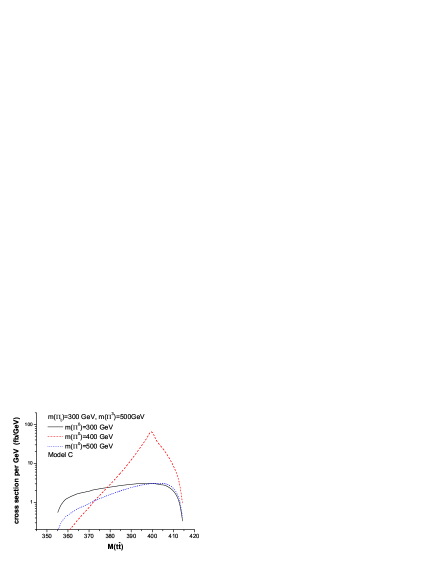
Figure 3: $t\bar{t}$ invariant mass distribution in Model C for $m_{\Pi_{t}}$=300 GeV and $m_{\Pi}$=300, 400, and 500 GeV.

In Figs. 3 and 4, we plot the $t\bar{t}$ invariant mass distributions in Model C for $m_{\Pi_{t}}=$ 300  and  400 GeV and $m_{\Pi^{0}}$= 300, 400, and 500 GeV. Again, we see the clear $\Pi^{0}$ resonance peak at 400 GeV, but the width of the resonance is much larger than that in Figs. 1 and 2 due to the largeness of the $\Pi^{0}\to{\rm gluons}$ and $\Pi^{0}\to t\bar{t}$ widths.

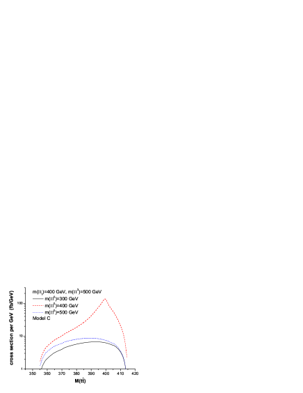
Figure 4: $t\bar{t}$ invariant mass distribution in Model C for $m_{\Pi_{t}}$=400 GeV and $m_{\Pi}$=300, 400, and 500 GeV.

In the case of $m_{\Pi_{t}}$=300 GeV, $N_{events}$ is $(5.2\--33)\times 10^{3}$. The corresponding $95\%$ C.L. statistical uncertainties are then $(1\--3)\%$. Compared with the large relative corrections $\Delta\sigma/\sigma_{0}$ listed in TABLE III, we see that the PGB effects in Model C can be clearly detected. Comparing the relative corrections $\Delta\sigma/\sigma_{0}$ listed in TABLE III and TABLE II, we see that the difference between Model C and Model B is significant for $m_{\Pi^{0}}$=300 and 400 GeV. For $m_{\Pi^{0}}$=500 GeV, the relative difference is $[\sigma(B)=\sigma(C)]/\sigma(B)=[109-104]/109=5\%$ which is also beyond the statistical uncertainties. Thus model C and Model B can be clearly distinguished from the production cross sections.

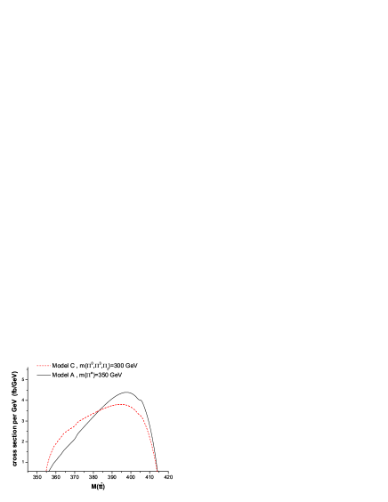
Figure 5: Comparison of the $t\bar{t}$ invariant mass distributions in Model C for $m_{\Pi_{t}}=m_{\Pi}=m_{\Pi_{a}}$=300 GeV and Model A for $m_{\Pi_{a}}=350$ GeV.

We see from TABLE III and TABLE I that, for most values of the PGB masses, Model C can be distinguished from Model A. The only case which needs to be studied more carefully is distinguishing the cases of Model C with $m_{\Pi_{t}}=m_{\Pi^{0}}$=300 GeV from Model A with $m_{\Pi_{a}}$=350$\--$400 GeV. From TABLE III and TABLE I, we see that the total cross sections for these two cases are almost the same, so that they cannot be distinguished by merely measuring the total cross sections. Since the numbers of events are around 8700$\--$8850, it is posiible to measure the $t\bar{t}$ invariant mass ($M_{t\bar{t}}$) distribution. In Fig. 5 we plot the $M_{t\bar{t}}$ distributions for the two cases.

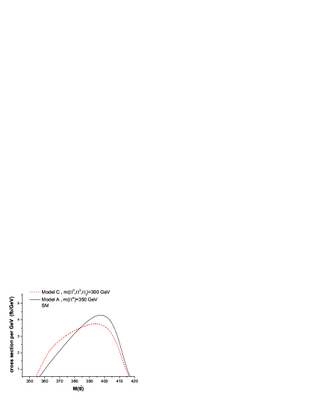
Figure 6: Comparison of the smeared $t\bar{t}$ invariant mass distributions in Model C for $m_{\Pi_{t}}=m_{\Pi}=m_{\Pi_{a}}$=300 GeV and Model A for $m_{\Pi_{a}}=350$ GeV according to the resolution ${\Delta E}/E=0.33/\sqrt{E}$.

To make it more realistic, we should furhter take into account the effect of energy resolution. According to Ref. TESLA-IV , the energy resolution is $\Delta E/E=0.33/\sqrt{E}$. We then smear the calculated $M_{t\bar{t}}$ by taking convolutions with this resolution. The obtained smeared $M_{t\bar{t}}$ distrobutions for the above two cases are shown in Fig. 6. We see that they are different, especially in the vicinities of 365 GeV and 400 GeV where the differences are of the level of $(10\--40)\%$. According to the energy resolution, the resolution for measuring the $M_{t\bar{t}}$ distribution around 400 GeV is $\Delta M_{t\bar{t}}=0.33\times\sqrt{400}~{}{\rm GeV}=6.6$ GeV. So that the above two cases in model A and Model C can be distinguished by separately measuring the numbers of events in the regions $355~{}{\rm GeV}\leq M_{t\bar{t}}\leq 375~{}{\rm GeV}$ and $390~{}{\rm GeV}\leq M_{t\bar{t}}\leq 410~{}{\rm GeV}$.

In the case of $m_{\Pi_{t}}$=400 GeV, we can see that Model C is very different from the SM, and all the three models can be distinguished.

In summary, we have studied the possibility of testing and distinguishing three improved technicolor models (Models A, B, and C) via $t\bar{t}$ productions at a polarized photon collider with $2\lambda_{e}P_{c}=-1$ from a 500 GeV $e^{+}e^{-}$ linear collider with an integrated luminosity of 500 fb^-1. The signal contains six jets from $t\to W^{+}b$ and $W\to q\bar{q}^{\prime}$. Backgronds can be suppressed by taking the cut (6) and tagging a $b$ quark jet. Considering the possible detection ability of the detector and the usual $b$-tagging efficiency, the detection efficiency is $10\%$. We see that, considering only the statistical error, the three improved technicolor models can all be well tested and can be distinguished from each other by measuring the $\gamma\gamma\to t\bar{t}$ production cross section and the $t\bar{t}$ invariant mass distribution.

Acknowledgement: We would like to thank C.-P. Yuan for discussions. This work is supported by the National Natural Science Foundation of China under the grant number 90103008.

References

- (1) S. Eidelman, al., (Particle Data Group), Phys. Lett. B 592, 1 (2004).
- (2) T. Appelquist and J. Terning, Phys. Lett. B 315, 139 (1993).
- (3) C.T. Hill, Phys. Lett. B 345, 483 (1995); K. Lane and E. Eichten, ibit. 352, 382 (1995); G. Buchalla, G. Burdan, C.T. Hill, and D. Kominis, Phys. Rev. D 53, 5185 (1996).
- (4) K. Lane, Phys. Lett. B 357, 624 (1995).
- (5) B. A. Dobrescu and C. T. Hill, Phys. Rev. Lett. 81, 2634 (1998); R. S. Chivukula, B. A. Dobrescu, H. Georgi, and C. T. Hill, Phys. Rev. D 59, 075003 (1999); H.-J. He, C. T. Hill, and T. Tait, Phys. Rev. D 65, 055006 (2002);
- (6) N. Arkani-Hammed, A.G. Cohen, and H. Georgi, Phys. Lett. B 513 (2001) 232; N. Arkani-Hammed, A.G. Chen, E. Katz, A.E. Nelson, T Gregoire, and J.G. Wacker, JHEP 0208 (2002) 021; J.G. Wacker, hep-ph/0208235; N. Arkani-Hammed, A.G. Cohen, E. Katz, and A.E. Nelson, JHEP 0207 (2002) 034; T. Gregoire and J.G. Wacker, hep-ph/0207164; I. Low, W. Skiba, and D. Smith, hep-ph/0207243.
- (7) H.-Y. Zhou, Y.-P. Kuang, C.-X. Yue, H. Wang, and G.-R. Lu, Phys. Rev. D 57, 4205 (1998).
- (8) C.-X. Yue, Y.-P. Kuang, X.-L. Wang, and W.B. Li, phys. Rev. D 62, 055005 (2000).
- (9) I.F.Ginzburg,G.L. Kotkin, S.L. Panfil, V.G. Serbo, and V.I. Telnov, Nucl. Instr. and Methods in Phys. Res. 219, 5 (1984); B. Badelek et al., Part VI of TESLA Technical Design Report, DESY 2001-011.
- (10) O.J.P. Ebóli et al., Phys. Rev. D 47, 1889 (1993); K. Cheung,, ibid. 47, 3750 (1993).
- (11) V.M. Budnev, I.F. Ginzburg, G.V. Meledin, and V.G. Serbo, Phys. Rep. 15 C, 181 (1975).
- (12) Particle Physics Experiments at JLC (JLC Technical Design Report), KEK Report 2001-11.
- (13) M. Baillargeon et al., in Collisions at TeV Energies: The Physics Potential, Part D, edited by P. Zerwas, DESY 96-123D (1995); see also Part VI of TESLA Technical Design Report, DESY 2001-011.
- (14) Part I of TESLA Technical Design Report, DESY 2001-011.
- (15) B. Balaji, Phys. Rev. D 53, 1699 (1996).
- (16) Part IV of TESLA Technical Design Report, DESY 2001-011.