UB-ECM-PF 04/37

The chiral structure of the Lamb shift and the definition of the proton radius
Antonio Pineda
Dept. d’Estructura i Constituents de la Matèria and IFAE, U. Barcelona
Diagonal 647, E-08028 Barcelona, Catalonia, Spain

The standard definition of the electromagnetic radius of a charged particle (in particular the proton) is ambiguous once electromagnetic corrections are considered. We argue that a natural definition can be given within an effective field theory framework in terms of a matching coefficient. The definition of the neutron radius is also discussed. We elaborate on the effective field theory relevant for the hydrogen and muonic hydrogen, specially for the latter. We compute the hadronic corrections to the lamb shift (for the polarizability effects only with logarithmic accuracy) within heavy baryon effective theory. We find that they diverge in the inverse of the pion mass in the chiral limit.

1 Introduction

The possibility to measure the muonic hydrogen ($\mu p$) Lamb shift at the 30 ppm level at the PSI [1] and, consequently, to obtain the proton radius with an improved accuracy of, at least, one order of magnitude better than current determinations, has triggered a lot of theoretical effort in order the theoretical errors to compete with the estimated experimental ones. We refer to [2, 3, 4] and references therein for a detailed explanation of the actual status of the art. On the other hand, it is also planed to study the muonic hydrogen properties at a future Neutrino Factory Complex [5].

Measuring the proton radius with such accuracy poses some theoretical questions on the definition of the proton radius. Actually, these problems already appear with the present claimed precision of around 1.5 % (see for instance [6]). The problem has to do with the fact that the proton radius is only defined at leading order in the electromagnetic coupling $\alpha$. Beyond this order, the usual definition through the use of form factors runs into problems because it becomes infrared divergent. This fact has already been discussed by Pachucki [7]. Here we address the problem using potential NRQED (pNRQED) [8, 9, 10], an effective field theory suited for the study of non-relativistic systems. We will closely follow Ref. [11], where the hyperfine splitting of the muonic hydrogen and the hydrogen ($ep$) was studied (we refer to this reference for further details, definitions and notation). Within this framework, and beyond leading order in $\alpha$, we will see that what one is really measuring is a matching coefficient of the effective theory, which is dependent on the scale (scheme) at which the matching has been performed.

On the other hand we will see that there is a series of hadronic contributions that can be computed using heavy baryon effective theory (HBET) [12]. In particular, the non-analytic (and model-independent) dependence on the light quark masses of the Lamb shift can be obtained. We will do so here for the Zemach and vacuum polarization piece of the hadronic correction. The polarizability corrections will only be considered with logarithmic accuracy. The full computation will be presented elsewhere.

2 Effective Field Theories

We will obtain pNRQED by passing through different intermediate effective field theories after integrating out different degrees of freedom. The path that we will take is the following:

$${\rm HBET}\rightarrow({\rm QED})\rightarrow{\rm NRQED}\rightarrow{\rm pNRQED},$$

much in the same way as we did in Ref. [11]. The fact that we are interested in the Lamb shift will force us to consider other operators which were not considered in that paper.

2.1 HBET

Our starting point is the SU(2) version of HBET coupled to leptons, where the delta is kept as an explicit degree of freedom. The degrees of freedom of this theory are the proton, neutron and delta, for which the non-relativistic approximation can be taken, and pions, leptons (muons and electrons) and photons, which will be taken relativistic. This theory has a cut-off $\mu<<m_{p}$, $\Lambda_{\chi}$ and much larger than any other scale in the problem. The Lagrangian can be split in several sectors. Most of them have already been extensively studied in the literature but some will be new. Moreover, the fact that some particles will only enter through loops, since only some specific final states are wanted, will simplify the problem. The Lagrangian can be written as an expansion in $e$ and $1/m_{p}$. and can be structured as follows

$${\cal L}_{HBET}={\cal L}_{\gamma}+{\cal L}_{l}+{\cal L}_{\pi}+{\cal L}_{l\pi}+{\cal L}_{(N,\Delta)}+{\cal L}_{(N,\Delta)l}+{\cal L}_{(N,\Delta)\pi}+{\cal L}_{(N,\Delta)l\pi},$$ (1)

representing the different sectors of the theory. In particular, the $\Delta$ stands for the spin 3/2 baryon multiplet (we also use $\Delta=m_{\Delta}-m_{p}$, the specific meaning in each case should be clear from the context).

Our aim is to obtain the Lamb shift with $O(m_{l_{i}}^{3}\alpha^{5}/m_{p}^{2}F(m_{l_{i}}/m_{\pi},m_{\pi}/\Delta)$ accuracy. In particular, we want to obtain the non-analytic behavior in the masses of the light quarks and in the $\Delta$. Actually, the full dependence on the ratio $m_{\pi}/\Delta$ can be obtained using chiral Lagrangians. In this paper we will mainly focus on a partial contribution to it: the so-called Zemach correction.

To obtain this accuracy, we need, in principle, Eq. (1) with $O(1/m_{p}^{2})$ accuracy. The different pieces of the Lagrangian can be found in Ref. [11]. There are a few differences due to the fact that we are now concerned with the Lamb shift correction. This implies that some terms in the nucleon Lagrangian, which were not considered in Ref. [11] have to be considered here. In particular, the term

$$\delta{\cal L}_{\gamma}=\left({d_{2,R}\over m_{p}^{2}}+{d_{2}^{(\tau)}\over m_{\tau}^{2}}\right)F_{\mu\nu}D^{2}F^{\mu\nu}\,,$$ (2)

where $d_{2,R}$ stands for the hadronic contribution. This term can be eliminated by field redefinitions (see for instance [13]) but we will keep it explicit since this contribution can be singled out by considering the lamb shift of a purely leptonic bound state.

For the nucleon there is a new term that has to be considered (actually in this one is where the proton radius is encoded):

$$\delta{\cal L}_{N}=N^{\dagger}_{p}\Biggl{\{}-e{c_{D}^{(p)}\over m_{p}^{2}}\left[{\bf\mbox{\boldmath$\nabla$}\cdot E}\right]\Biggr{\}}N_{p}\,.$$ (3)

Specially relevant in our case is $c_{3,R}^{pl_{i}}$ (see Eq. (14) in [11]). Nevertheless, the leading contribution in $\alpha$ (of $O(\alpha^{2})$) is suppressed by an extra factor $m_{l_{i}}/m_{p}$ (see Eq. (39)), i.e. $c_{3,R}^{pl_{i}}\sim\alpha^{2}m_{l_{i}}/m_{p}$, which goes beyond the aimed accuracy of our calculation and we can neglect it.

2.2 NRQED

Since we want to obtain corrections to the lamb shift, besides the operators considered in Ref [11] new operators have to be considered with $O(1/(m_{p}^{2}m_{\pi}))$ precision. This means that some operators of up to dimension 7 have to be included in the Lagrangian. They read

$$\delta{\cal L}_{N}=N^{\dagger}_{p}\Biggl{\{}c^{(p)}_{A_{1}}\,{e^{2}}\,{{\bf B}^{2}-{\bf E}^{2}\over 8m_{p}^{3}}-c^{(p)}_{A_{2}}\,{e^{2}}\,{{\bf E}^{2}\over 16m_{p}^{3}}\Biggr{\}}N_{p}\,.$$ (4)

$c_{A_{1}}^{(p)}$, $c_{A_{2}}^{(p)}$ correspond to the proton polarizabilites. The relations are the following:

$$c_{A_{1}}^{(p)}=4m_{p}^{3}{\beta_{M}^{(p)}\over\alpha}\,,\qquad c_{A_{2}}^{(p)}=-{8m_{p}^{3}\over\alpha}(\alpha_{E}^{(p)}+\beta_{M}^{(p)}).$$ (5)

We also note that the operators considered in Eqs. (2) and (3) also appear here. In the first case $d_{2,R}\rightarrow d_{2,NR}$. $d_{2,NR}$ is scale independent but pion effects should be included now. We will discuss in further detail these corrections in sec. 4. $c_{D}^{(p)}(\nu)$ is a matching-scale dependent quantity and has already been considered in HBET. The difference is the scale $\nu$ considered in each case, whereas in HBET $m_{\pi}\ll\nu\ll m_{p}$, we now have $m_{l_{i}}\alpha\ll\nu\ll m_{\pi}$. This means that in HBET, effects due to the pion scale were not included in $c_{D}^{(p)}(\nu)$ but now they are. A similar discussion applies to $c_{3,NR}^{pl_{i}}(\nu)$ (see Eq. (17) in Ref. [11]), which is also scale dependent.

2.3 pNRQED

After integrating out scales of $O(m_{l_{i}}\alpha)$ one ends up in a Schrödinger-like formulation of the bound-state problem. We refer to [8, 9, 10] for details. The pNRQED Lagrangian for the $ep$ (the non-equal mass case) can be found in Appendix B of [10] up to $O(m\alpha^{5})$. The pNRQED Lagrangian for the $\mu p$ is similar except for the fact that light fermion (electron) effects have to be taken into account. The explicit form of the Lagrangian has not been presented so far. We do so here. The explicit Lagrangian reads (up to $O(m\alpha^{5})$)

$$L_{pNRQED}=\int d^{3}{\bf x}d^{3}{\bf X}S^{\dagger}({\bf x},{\bf X},t)\Biggl{\{}i\partial_{0}-{{\bf p}^{2}\over\mu_{12}}+{{\bf p}^{4}\over 8m_{\mu}^{3}}+{{\bf p}^{4}\over 8m_{p}^{3}}-{{\bf P}^{2}\over 2M}$$ (6)

$$-V({\bf x},{\bf p},{\mbox{\boldmath$\sigma$}}_{1},{\mbox{\boldmath$\sigma$}}_{2})+e{\bf x}\cdot{\bf E}({\bf X},t)\Biggr{\}}S({\bf x},{\bf X},t)-\int d^{3}{\bf X}{1\over 4}F_{\mu\nu}F^{\mu\nu}\,,$$

where $M=m_{\mu}+m_{p}$, $\mu_{12}={m_{\mu}m_{p}\over m_{\mu}+m_{p}}$, ${\bf x}$ and ${\bf X}$, and ${\bf p}$ and ${\bf P}$ are the relative and center of mass coordinate and momentum respectively.

$V$ can be written as an expansion in $1/m_{\mu}$, $1/m_{p}$, $\alpha$, … We will assume $1/r\sim m_{e}$ (which is realistic for the case at hand) and concentrate in the $1/m_{\mu}$ expansion. We assume that $m_{\mu}<<m_{p}$.

$$V({\bf x},{\bf p},{\mbox{\boldmath$\sigma$}}_{1},{\mbox{\boldmath$\sigma$}}_{2})=V^{(0)}(r)+{V^{(1)}(r)\over m_{\mu}}+{V^{(2)}(r)\over m_{\mu}^{2}}+\,.\,.\,.$$ (7)

In order to reach the desired NNNLO accuracy in $\alpha_{s}$, $V^{(0)}$ has to be computed up to $O(\alpha^{4})$, $V^{(1)}$ up to $O(\alpha^{3})$, $V^{(2)}$ up to $O(\alpha^{2})$ and $V^{(3)}$ up to $O(\alpha)$. Nevertheless, there is not contribution to $V^{(3)}$ at tree level. We first write the potential up to order $1/m_{\mu}^{2}$ in momentum space.
Order $1/m^{0}$. We define ${\tilde{V}}^{(0)}$ (the Fourier transform of $V^{(0)}$):

$${\tilde{V}}^{(0)}\equiv-4\pi Z_{\mu}Z_{p}\alpha_{V}(k){1\over{\bf k}^{2}},$$ (8)

which in fact defines $\alpha_{V}$, which is gauge invariant. There is another very popular definition that enjoys all the nice properties we would like $\alpha$ to have (gauge invariance,scheme/scale independence…):

$$\alpha_{eff}(k)=\alpha{1\over 1+\Pi(-{\bf k}^{2})}\,,$$ (9)

where

$$\Pi(k^{2})=\alpha\Pi^{(1)}(k^{2})+\alpha^{2}\Pi^{(2)}(k^{2})+\alpha^{3}\Pi^{(3)}(k^{2})+...$$

is the electron vacuum polarization and $\Pi(0)=0$. $\alpha_{eff}$ corresponds to Dyson summation. If we express $\alpha_{V}(k)$ in terms of $\alpha_{eff}(k)$, we have

$$\alpha_{V}(k)=\alpha_{eff}(k)+\sum_{n,m=0\atop n+m=even>0}Z_{\mu}^{n}Z_{p}^{m}\alpha_{eff}^{(n,m)}(k)=\alpha_{eff}(k)+\delta\alpha(k)\,,\quad\quad\delta\alpha(k)=O(\alpha^{4}).$$ (10)

The sum is constrained to fulfill $n+m=even$ because of the Furry theorem. Each $\alpha_{eff}^{(n,m)}(k)$ is also gauge invariant. In order to achieve $O(m\alpha^{5})$ accuracy we need to know $\Pi^{(1)}$, $\Pi^{(2)}$, $\Pi^{(3)}$ (see [14]) and the leading, non-vanishing, contributions to $\alpha_{eff}^{(2,0)}(k)$, $\alpha_{eff}^{(0,2)}$ and $\alpha_{eff}^{(1,1)}$. A discussion on the latter (which still remain to be computed) can be found in Ref. [15].

As we have already mentioned, the matching is performed in a expansion in $1/m$, $\alpha$ and the energy. The leading-non-zero contribution to the potential from the expansion in the energy appears at $O(1/m^{0})$ and $O(\alpha^{2})$ and it will give rise to a contribution of $O(m\alpha^{5})$. It follows from the electron vacuum polarization correction to the potential shown in Fig. 1. In momentum space it reads

$$\delta{\tilde{V}}_{VP}=Z_{\mu}Z_{p}e^{2}{1\over{\bf k}^{2}}\pi(k^{2})\,,$$ (11)

where $\pi(k^{2})=\alpha\Pi^{(1)}(k^{2})$. We note that this correction depends on $k_{0}$. Since $k_{0}\sim m\alpha^{2}$ and ${\bf k}\sim m\alpha$ we can expand in ${k^{2}_{0}\over{\bf k}^{2}}$. The leading order is $k_{0}$ independent and produces the standard vacuum polarization correction that we have already taken into account in $\alpha_{eff}$:

$$Z_{\mu}Z_{p}e^{2}{1\over{\bf k}^{2}}\pi(-{\bf k}^{2})\,.$$ (12)

The next correction reads

$$\delta{\tilde{V}}_{E}=Z_{\mu}Z_{p}e^{2}{k^{2}_{0}\over{\bf k}^{2}}\pi^{\prime}(-{\bf k}^{2})\,,$$ (13)

and is new.

(50,30) i1,o1 i2,o2 fermion,width=thick,label=$E_{1},,\;{\bf p}$,label.side=lefti1,v1 fermion,width=thick,label=$E_{1}^{\prime},,\;{\bf p}^{\prime}$, label.side=leftv1,o1 fermion,width=thicki2,v2,o2 dashes,width=thinv1,v3,v2 l=$k_{0},,\;{\bf k}$,l.a=180,label.dist=.2w,decoration.shape=circle,d.f=empty,d.si=.2wv3

Figure 1: Leading correction to the Coulomb potential due to the electron vacuum polarization in the Coulomb gauge. ${\bf k}={\bf p}-{\bf p}^{\prime}$ and $k_{0}=E_{1}-E_{1}^{\prime}$.

The explicit expression of $\pi$ reads

$$\pi(k^{2})={\alpha\over\pi}k^{2}\int_{4}^{\infty}d(q^{2}){1\over q^{2}(m_{e}^{2}q^{2}-k^{2})}u(q^{2})\,,$$ (14)

where

$$u(q^{2})={1\over 3}\sqrt{1-{4\over q^{2}}}\left(1+{2\over q^{2}}\right)\,.$$

The $k_{0}$ dependence in the potential translates into terms with time derivatives in the pNRQED Lagrangian (or in other words an energy dependent potential). At the order we are working, one can get rid of these time derivatives by using the equations of motion. Note that we refer to the full equations of motion (including the potential), and not just the equations of motion of free particles, reflecting the fact that the matching has to be done off-shell. The procedure has been illustrated in the Appendix A of [10]. Effectively, this transforms $\delta{\tilde{V}}_{E}$ into the following expression

$$\delta{\tilde{V}}_{E}=-{Z_{\mu}Z_{p}e^{2}\over 4m_{\mu}m_{p}}{({\bf p}^{2}-{\bf p}^{\prime\,2})^{2}\over{\bf k}^{2}}{\alpha\over\pi}m_{e}^{2}\int_{4}^{\infty}d(q^{2}){1\over(m_{e}^{2}q^{2}+{\bf k}^{2})^{2}}u(q^{2})\,.$$ (15)

We see that it becomes a $O(1/m^{2})$ potential. Field redefinitions should produce an equivalent result. We note that if we want to go to higher orders than $O(m\alpha^{5})$, we should work with the former expression Eq. (13), or work in a more general way by using field redefinitions.

Order $1/m$. They will give rise to $O(m\alpha^{6})$ corrections so they will be neglected in the following.

Order $1/m^{2}$. At the order we are working they can be written as follows:

$${\tilde{V}}^{(b)}={\pi\alpha_{eff}(k)\over 2}\left[Z_{p}{c_{D}^{(\mu)}\over m_{\mu}^{2}}+Z_{\mu}{c_{D}^{(p)}\over m_{p}^{2}}\right]\,,$$ (16)

$${\tilde{V}}^{(c)}=-i2\pi\alpha_{eff}(k){({\bf p}\times{\bf k})\over{\bf k}^{2}}\cdot\left\{Z_{p}{c_{S}^{(\mu)}{\bf s}_{1}\over m_{\mu}^{2}}+Z_{\mu}{c_{S}^{(p)}{\bf s}_{2}\over m_{p}^{2}}\right\}\,,$$ (17)

$${\tilde{V}}^{(d)}=-Z_{\mu}Z_{p}16\pi\alpha\left({d_{2}^{(\mu)}\over m_{\mu}^{2}}+{d_{2}^{(\tau)}\over m_{\tau}^{2}}+{d_{2,NR}\over m_{p}^{2}}\right)\,,$$ (18)

$${\tilde{V}}^{(e)}=-Z_{\mu}Z_{p}{4\pi\alpha_{eff}(k)\over m_{\mu}m_{p}}\left({{\bf p}^{2}\over{\bf k}^{2}}-{({\bf p}\cdot{\bf k})^{2}\over{\bf k}^{4}}\right)\,,$$ (19)

$${\tilde{V}}^{(f)}=-{i4\pi\alpha_{eff}(k)\over m_{\mu}m_{p}}{({\bf p}\times{\bf k})\over{\bf k}^{2}}\cdot(Z_{p}c_{F}^{(\mu)}{\bf s}_{1}+Z_{\mu}c_{F}^{(p)}{\bf s}_{2})\,,$$ (20)

$${\tilde{V}}^{(g)}={4\pi\alpha_{eff}(k)c_{F}^{(1)}c_{F}^{(2)}\over m_{\mu}m_{p}}\left({\bf s}_{1}\cdot{\bf s}_{2}-{{\bf s}_{1}\cdot{\bf k}{\bf s}_{2}\cdot{\bf k}\over{\bf k}^{2}}\right)\,,$$ (21)

$${\tilde{V}}^{(h)}=-{1\over m_{p}^{2}}\left\{(c_{3,NR}^{pl_{i}}+3c_{4,NR}^{pl_{i}})-2c_{4,NR}^{pl_{i}}{\bf S}^{2}\right\}\,.$$ (22)

The classification of the diagrams follows the one of Fig. 1 of Ref. [10] generalized to the non-equal mass case and with the replacement $\alpha\rightarrow\alpha_{eff}$. This ensures that the expressions for the potentials are correct at one-loop (the one-loop vacuum polarization is included). Written in this way subleading terms in $\alpha$ are also included. It should be keep in mind that at some point the replacement of $\alpha$ by $\alpha_{eff}$ is not enough and new corrections have to be included in the potentials.

$$d_{2,NR}=d_{2,R}+{m_{p}^{2}\over 4}\Pi^{\prime}_{h,\pi}(0)={m_{p}^{2}\over 4}\Pi^{\prime}_{h}(0)\,,$$ (23)

where $\Pi^{\prime}_{h}(0)$ is the derivative of the hadronic vacuum polarization (we have defined $\Pi_{h}(-{\bf k}^{2})=-{\bf k}^{2}\Pi^{\prime}_{h}(0)+\,.\,.\,.$) and $\Pi^{\prime}_{h,\pi}(0)$ is the contribution due only to pions.

The one loop diagrams of fig. 2 of Ref. [10] are equal in our case up to a trivial mass rescaling:

$${\tilde{V}}^{(a)}_{1loop}={Z_{\mu}^{2}Z_{p}^{2}\alpha^{2}\over m_{\mu}m_{p}}\left(\log{{\bf k}^{2}\over\mu^{2}}-{8\over 3}\log 2+{5\over 3}\right)\,,$$ (24)

$${\tilde{V}}^{(b,c)}_{1loop}={4Z_{\mu}^{2}Z_{p}^{2}\alpha^{2}\over 3m_{\mu}m_{p}}\left(\log{{\bf k}^{2}\over\mu^{2}}+2\log 2-1\right)\,.$$ (25)

The procedure we have followed to obtain the potentials is different from the one used in Ref. [2]. For instance, in this last reference no mention to a correction to the type of Eq. (15) is made. To facilitate the comparison one should work in position space (it is also eventually useful to write the potential in a basis where the angular momentum structure of the potential is more visible). The non-trivial comparison can be reduced to the contribution due to $\delta{\tilde{V}}_{E}$ and the one-loop correction to ${\tilde{V}}^{(e)}$, which in our case reads

$$\left.\delta V_{E}+V^{(e)}\right|_{1\rm loop}=-{Z_{\mu}Z_{p}\alpha^{2}\over\pi}{m_{e}^{2}\over m_{\mu}m_{p}}\int_{4}^{\infty}d(q^{2}){u(q^{2})\over(m_{e}q)^{2}}\left\{{1\over 2}\left\{{\bf p}^{2},{e^{-m_{e}qr}\over r}\left(1+{m_{e}qr\over 2}\right)\right]\right\}$$

$$-{e^{-m_{e}qr}\over 2r^{3}}\left(1+m_{e}qr\right){\bf L}^{2}\left.+{(m_{e}q)^{2}\over 4r}e^{-m_{e}qr}\left(1+{m_{e}qr\over 2}\right)-2\pi\delta(\bf r)\right\}\,,$$ (26)

where ${\bf L}$ is the angular momentum. We have checked that this expression agrees with the corresponding expression in Ref. [2].

In this paper, our main focus are the hadronic corrections, in particular those proportional to the $\delta(\bf r)$ potential. They can be encoded in the matching coefficient of the spin-independent delta potential:

$$\delta V={D_{d}^{\rm had}\over m_{p}^{2}}\delta^{(3)}({\bf r})\,.$$ (27)

where

$$D_{d}^{\rm had}\equiv-c_{3,NR}^{pl_{i}}-16\pi\alpha Z_{l_{i}}Z_{p}d_{2,NR}+{\pi\alpha\over 2}Z_{l_{i}}c_{D}^{(p)}\,.$$ (28)

The spin-dependent term does not contribute to the average energy over polarizations. Therefore the hadronic contribution to the lamb shift reads

$$\delta E=\langle E(s)-E(p)\rangle={D_{d}^{\rm had}\over m_{p}^{2}}\delta_{l0}{1\over\pi}\left({\mu_{l_{i}p}\alpha\over n}\right)^{3}\,.$$ (29)

3 Definition of the proton radius

The usual definition of the electromagnetic radius of the proton is the following

$$r^{2}_{p}=6\left.{dG_{p,E}(q^{2})\over d\,q^{2}}\right|_{q^{2}=0}\,.$$ (30)

This definition runs into problem once electromagnetic corrections are included in the computation of $G_{p,E}$ because it becomes infrared divergent (this is so for a charged particle, for the neutron this definition is infrared safe). This problem has already been pointed out in Ref. [2]. Nevertheless, this is not a problem from the effective theory point of view, where the parameters of the theory (the matching coefficients) do depend in general on the scheme and scale on which the computation has been performed. Therefore, our definition of the proton radius is the following

$$c_{D}^{(p)}-1\equiv{4\over 3}r_{p}^{2}m_{p}^{2}\,,$$ (31)

which naturally relates to the one in Eq. (30), since

$$c_{D}=1+2F_{2}+8F_{1}^{\prime}=1+8m_{p}^{2}\left.{dG_{p,E}(q^{2})\over d\,q^{2}}\right|_{q^{2}=0}\,,$$ (32)

where we have already used that $F_{1}=1$ due to gauge invariance. Eq. (31) is the natural definition from the point of view of effective field theory (a matching coefficient). Another issue is the separation of ”hadronic” from electromagnetic corrections. We stress that the electromagnetic effects are included in the form factors above. We note that $r_{p}$ is now an scale dependent quantity and fulfils an expansion in $\alpha$:

$$r_{p}(\nu)=r_{p}^{(0)}+\alpha r_{p}^{(1)}(\nu)+\cdots\,.$$ (33)

We will define the pure hadronic definition of the radius (”hadronic proton electromagnetic radius”) to be the first term in this expansion, $r_{p}^{(0)}$. Note that this quantity is not an observable from the effective field theory point of view, since it will always appear (in the same combination) with another hadronic corrections in the observable. This definition for the ”hadronic” piece is different in general of the definition in [16].

We can also know what the running of each term of $r_{p}$ is. As we have already mentioned, the first term is scale independent but not the second (even if this running can be understood in terms of point-like particles).

$$\nu{d\over d\nu}r_{p}^{(0)}=0\,,\quad r_{p}^{(0)}\nu{d\over d\nu}r_{p}^{(1)}=-{1\over\pi}{1\over m_{p}^{2}}\,,\quad\cdots\,.$$ (34)

In summary, if we give a number for the proton radius we have to say in which scheme (for instance $\overline{\rm MS}$) and scale it has been obtained if a precision of around 1 % is claimed. In Ref. [7] a prescription has been taken to fix the ambiguity with $O(\alpha)$ precision (how to generalize this prescription to higher orders in $\alpha$ is left unsettled). There, the scale dependence at $O(\alpha)$ is regulated by the proton mass and the finite pieces fixed by performing the computation assuming the proton to be point-like at scales of order $m_{p}$. Nevertheless, this assumption is not justified since at these scales several resonances appear. We would also like to stress that our definition of the proton radius through a matching coefficient, $c_{D}^{(p)}$, makes easier to obtain the dependence of any observable in this quantity, in particular for the cross section $\sigma(e^{-}p\rightarrow e^{-}p)$.

What we have said is quite general for any nucleus. Indeed, the object which is really measured at very low momentum transfer (above or below threshold) between the nucleus and lepton is $D_{d}(\nu)=D_{d}^{\rm lep}+D_{d}^{\rm had}$. Therefore, one could think that it is more proper to give numbers for this object (for a given scale and scheme). Nevertheless, if we want to get some understanding on the structure of the nucleus it maybe convenient to distinguish the different hadronic and leptonic contributions of $D_{d}(\nu)$ as some of them can be singled out from different measurements. For instance the contribution due to $d_{2,NR}$, as well as the leptonic contributions, can be singled out since they can be computed explicitly and measured changing the nucleus by another lepton. Moreover, it also makes some sense to distinguish between $c_{3,NR}^{pl_{i}}$ and $c_{D}^{(p)}$ (at least at $O(\alpha^{2}m_{l_{i}})$), since the leading dependence on $c_{3,NR}^{pl_{i}}$ is proportional to the lepton mass and can be distinguished by changing the lepton. Beyond $\alpha^{2}$ or beyond $m_{l_{i}}$, this distinction is not that clear and can not be achieved in general. This has to do with the fact that we are not working in a minimal basis of operators in the effective Lagrangian. In other words, one can always perform a field redefinition to eliminate $c_{D}^{(p)}$, which gets absorbed in $c_{3,NR}$. Therefore, in the long term one should work with $D_{d}^{\rm had}$, which can be related with observable quantities (for the neutron case it can easily be related with the scattering lengths).

4 Matching HBET to NRQED

The hadronic corrections to the spin-independent delta potential are encoded in the corrections to $d_{2,NR}$, $c_{D}^{(p)}$ and $c_{3,NR}$.

We will only compute the hadronic corrections to $d_{2,NR}$ and $c_{3,NR}$ (due to energies of $O(m_{\pi},\Delta)$), since our aim is to obtain $c_{D}^{(p)}$ from experiment (for instance, from the muonic hydrogen lamb shift). If we were interested in $r_{p}^{(0)}$ one should also compute the hadronic $O(\alpha)$ corrections to $c_{D}^{(p)}$.

The leading correction to $d_{2,NR}$ is due to the one-loop pion correction to the vacuum polarization. The diagram that contributes at leading order is the same than in Fig. 1 changing the electron by a pion in the limit of transfer momentum going to zero. It reads

$$\Pi^{\prime}_{h,\pi}(0)={\alpha\over 30\pi}{1\over 4m_{\pi}^{2}}\,.$$ (38)

b

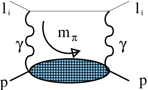
Figure 2: Symbolic representation of Eq. (39).

The contribution to $c_{3,NR}$ (see Fig. 2) can be written in a compact way in terms of the form factors of the forward virtual-photon Compton tensor (see [11] for details). It reads (this expression is only valid in 4 dimensions and in $D$-dimensions has to be properly generalized)

$$c_{3,NR}^{pl_{i}}=ig^{4}m_{p}m_{l_{i}}\int{d^{4}k\over(2\pi)^{4}}{1\over k^{4}}{1\over k^{4}-4m_{l_{i}}^{2}k_{0}^{2}}\left\{S_{1}(k_{0},k^{2})(-3k_{0}^{2}+{\bf k}^{2})-{\bf k}^{2}S_{2}(k_{0},k^{2})\right\}\,.$$ (39)

This result keeps the complete dependence on $m_{l_{i}}$. This contribution is usually organized in the following way

$$c_{3,NR}^{pl_{i}}=c_{3,R}^{p}+\delta c_{3,point-like}^{pl_{i}}+\delta c_{3,Zemach}^{pl_{i}}+\delta c_{3,pol.}^{pl_{i}}\,.$$ (40)

We remind that $c_{3,R}^{p}$ is $O(\alpha^{2}m_{l_{i}}/m_{p})$ and can be neglected. The second term corresponds to the diagram assuming the proton non-relativistic and point-like. With the precision needed it reads (in the $\overline{\rm MS}$ scheme)

$$\delta c_{3,point-like}^{pl_{i}}={m_{p}\over m_{l_{i}}}\left(\ln{m_{l_{i}}^{2}\over\nu^{2}}+{1\over 3}\right)\,.$$ (41)

b

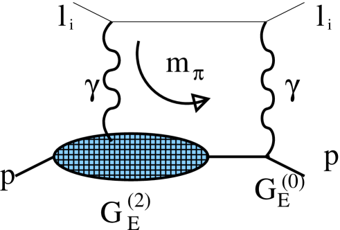
Figure 3: Symbolic representation (plus permutations) of the Zemach correction in Eq. (42).

The second term in Eq. (40) is the so-called Zemach correction, which is one of the main concerns of this paper. It is symbolically pictured in Fig. 3 and reads

$$\delta c_{3,Zemach}^{pl_{i}}=4(4\pi\alpha)^{2}m_{p}^{2}m_{l_{i}}\int{d^{D-1}k\over(2\pi)^{D-1}}{1\over{\bf k}^{6}}G_{E}^{(0)}G_{E}^{(2)}\,.$$ (42)

This term appears to be finite to the order of interest (it produces no logs) and it agrees with the result obtained by Pachucki [2] at leading order. Note, that this result holds for both ep and $\mu p$. In other words, the exact dependence on $m_{l_{i}}$ is kept. $G_{E}^{(0)}=1$. We take the expression for $G_{E}^{(2)}$ from [17]. The use of effective field theories and dimensional regularization is a strong simplification: we only need the non-analytic behavior of $G_{E}^{(2)}$ in $q^{2}$, the analytical behavior produces scaleless integrals, which are zero in dimensional regularization. This is a reflection of the factorization of the different scales. We do not need to introduce the point-like interactions to regulate the infrared divergences of the integrals at zero momentum. A similar thing happened [11] for the computation of the hyperfine splitting of the hydrogen, where, again, there was not not need to introduce the point-like interactions to regulate the infrared divergences of the integrals at zero momentum.

The result of the computation reads

$$\delta c_{3,Zemach}^{pl_{i}} = {2}(\pi\alpha)^{2}\left({m_{p}\over 4\pi F_{0}}\right)^{2}{m_{l_{i}}\over m_{\pi}}\left\{{3\over 4}g_{A}^{2}+{1\over 8}\right.$$

$$\left.+{2\over\pi}g_{\pi N\Delta}^{2}{m_{\pi}\over\Delta}\sum_{r=0}^{\infty}C_{r}\left({m_{\pi}\over\Delta}\right)^{2r}+g_{\pi N\Delta}^{2}\sum_{r=1}^{\infty}H_{r}\left({m_{\pi}\over\Delta}\right)^{2r}\right\}\,,$$

where

$$C_{r}={(-1)^{r}\Gamma(-3/2)\over\Gamma(r+1)\Gamma(-3/2-r)}\left\{B_{6+2r}-{2(r+2)\over 3+2r}B_{4+2r}\right\}\,,\qquad r\geq 0\,,$$ (44)

and the definition of $B_{n}$ and $H_{n}$ can be found in Appendix A. The term proportional to $B_{n}$ are due to scales of $O(\Delta)$, the contributions proportional to $H_{n}$ are due to scales of $O(m_{\pi})$. We see that the latter give contributions to the Lamb shift which are non-analytical in the quark mass.

We have then obtained the leading correction to the Zemach term in the chiral counting (supplemented with a large $N_{c}$ counting). This is a model independent result. Other contributions to the Zemach term are suppressed in the chiral counting.

b

Figure 4: Diagram contributing to the polarizability correction with $\ln m_{e}$ accuracy. The matching coefficients of the proton can be $c_{A_{1}}$ or $c_{A_{2}}$, or, in other words, the proton polarizabilities.

Finally, we consider the polarizability corrections. For those we would need the full expression for the virtual-photon Compton tensor at one-loop in HBET, which is lacking at present. This computation is relegated to a future publication. We will only consider here the limit $m_{l_{i}}\ll m_{\pi}$, which is relevant for the hydrogen atom, and only consider the logarithm ($\ln m_{e}$) enhanced terms. These can be obtained by computing the ultraviolet behavior of the diagram in Fig. 4. This contribution is proportional to $c_{A_{1}}$ and $c_{A_{2}}$. It can be written in term of the polarizabilites of the proton (see [18, 19])

$$\delta c_{3,pol}^{pl_{i}}=-\alpha m_{p}^{2}m_{l_{i}}\left[5\alpha_{E}^{(p)}-\beta_{M}^{(p)}\right]\ln({m_{l_{i}}})\,.$$ (45)

For the pure pion cloud, the polarizabilities were computed in Ref. [20]. The contribution due to the $\Delta$ can be found in Ref. [21]. The scale in the logarithm is compensated by the next scale of the problem, which can be $m_{\pi}$ or $\Delta$. For contributions which are only due to the $\Delta$ or pions, the scale is unambigous. In the case where pions and $\Delta$ are both present in the loop we will choose the pion mass (the difference being beyond the logarithmic accuracy). The result reads

$$\delta c_{3,pol}^{pl_{i}} = -{2\over 9}\alpha^{2}{m_{l_{i}}\over\Delta}b_{1,F}^{2}\ln{\Delta\over m_{l_{i}}}+{49\over 12}\pi\alpha^{2}g_{A}^{2}{m_{l}\over m_{\pi}}{m_{p}^{2}\over(4\pi F_{0})^{2}}\ln({m_{\pi}\over m_{l}})$$

$$+{8\over 27}\alpha^{2}g_{\pi N\Delta}^{2}{m_{l}\over\sqrt{\Delta^{2}-m_{\pi}^{2}}}{m_{p}^{2}\over(4\pi F_{0})^{2}}\left({45\Delta\over\sqrt{\Delta^{2}-m_{\pi}^{2}}}+{4\Delta^{2}-49m_{\pi}^{2}\over\Delta^{2}-m_{\pi}^{2}}\ln R\right)\ln({m_{\pi}\over m_{l}})\,,$$

where

$$R={\Delta\over m_{\pi}}+\sqrt{{\Delta^{2}\over m_{\pi}^{2}}-1}\,.$$ (47)

We would like to stress here that some of the corrections considered in Eq. (4) are missing in the dipole approximation [22], which is sometimes used in the literature. For instance, the first term in Eq. (4) (the pure Delta correction) would be missing in that approximation.

5 Phenomenological analysis

Our aim here is to see how much of the hadronic correction can be understood in terms of the physics of the $m_{\pi}$ and/or $\Delta$ scales.

There have been some previous estimates [2, 3, 23] of the Zemach correction using phenomenological model parameterizations of the proton form factors. They obtain quite similar numbers. For instance, using the dipole parameterization of the proton form factor,

$$G_{E}({\bf q}^{2})={1\over\left(1+\displaystyle{{\bf q}^{2}\over\Lambda^{2}}\right)^{2}}\,,$$ (48)

Pachucki [2] obtains 0.021 meV (slightly larger in [3] or if one takes into account relativistic effects) using $\Lambda=848.5$ MeV. Within chiral perturbation theory, the Zemach correction to the muonic hydrogen Lamb shift in the limit $\Delta\rightarrow\infty$ reads

$$\left.\delta E_{\mu p}^{\rm Zemach}(n=2)\right|_{\Delta\rightarrow\infty}=-0.01008\,{\rm meV}\,.$$ (49)

This is around 1/2 the standard predictions using the phenomenological parameterization of the form factors. The inclusion of the effects due to the $\Delta$ increase this number by around a factor of two and bring it surprisingly close to the phenomenological estimates.

$$\delta E_{\mu p}^{\rm Zemach}(n=2)=-0.01922\,{\rm meV}\,.$$ (50)

The corrections due to the Delta are large even if the series in $m_{\pi}/\Delta$ is convergent ($-0.01008-0.00561+\cdots$). It would be interesting to study whether something similar happens for the hyperfine splitting.

Obviously, for the hydrogen we also obtain similar numbers to the phenomenological estimates if the $\Delta$ is included

$$\delta E_{ep}^{\rm Zemach}(n=2)=-3.49652\,{\rm Hz}\,.$$ (51)

The pure pionic correction reads

$$\left.\delta E_{ep}^{\rm Zemach}(n=2)\right|_{\Delta\rightarrow\infty}=-1.83404\,{\rm Hz}\,.$$ (52)

The polarizability correction shown in sec. 4 is only reliable for the case of hydrogen. It is proportional to the electric and magnetic proton polarizabilities. Therefore, the question is how good HBET can reproduce the experimental number for the polarizabilities. Actually, if only the pure ”pionic” contribution is included a very good agreement is obtained. This agreement is deteriorated if corrections due to the $\Delta$ are included (specially for $\beta_{M}$). In any case, the correction we obtain for the Lamb shift correction reads

$$\left.\delta E_{ep}^{\rm pol.}\right|_{\Delta\rightarrow\infty}=-\frac{64.4841}{n^{3}}\,{\rm Hz}\,,$$ (53)

and including the $\Delta$

$$\delta E_{ep}^{\rm pol.}=-\frac{77.6037}{n^{3}}\,{\rm Hz}\,.$$ (54)

We see that they are reasonable close to each other and with the value obtained using the experimental number for the proton polarizabilites [19]. Slightly larger numbers are obtained using the experimental data of the deep inelastic structure functions [23] or models [24].

Finally, we would like to stress that in our determination there is no free parameter. The leading contribution is the one we have computed. This is due to the chiral enhancement. Our result diverges in the chiral and/or $1/N_{c}$ limit.

For the vacuum polarization, the contribution due to the pion loop is numerically small (even if leading from the power counting point of view). One obtains $\Pi_{h,\pi}^{\prime}\simeq 1.0\times\,10^{-3}\,{\rm GeV}^{-2}$. This should be compared with the experimental figure for the total hadronic contribution $\Pi_{h}^{\prime}\simeq 9.3\times\,10^{-3}\,{\rm GeV}^{-2}$ [25]. Actually, the main contribution comes from the $\rho$ even if it is suppressed in the power counting ($\sim 6.1\times\,10^{-3}\,{\rm GeV}^{-2}$). In any case we need $\Pi_{h}^{\prime}$ with $(\alpha/m_{p}^{2})$ precision for which we can take the experimental number for the vacuum polarization (matching coefficient $d_{2,NR}$) and the correction to the Lamb shift reads

$$\delta E_{ep}^{\rm vac.\;pol.}=-{3.39990\over n^{3}}\,{\rm kHz}\,,\qquad\delta E_{\mu p}^{\rm vac.\;pol.}=-{0.09039\over n^{3}}\,{\rm meV}\,,$$ (55)

which for the hydrogen case reduces to the result obtained in Ref. [26].

6 Conclusions

We have studied the lamb shift of hydrogen and muonic hydrogen within an effective field theory framework, connecting the physics at the hadronic scale (HBET) with the physics at the atomic scale (pNRQED). We have focused on the hadronic corrections and showed that a natural definition of the proton radius can be given as a matching coefficient of the effective theory.

The leading hadronic corrections to the Lamb shift are a prediction of HBET (unknown couterterms are subleading). We have exactly computed them for the Zemach and vacuum polarizability terms, and for the polarizability term with logarithmic accuracy. For the Hydrogen atom the computed correction is beyond the present experimental accuracy. Nevertheless, the result is perfectly relevant for the muonic hydrogen, for which it would be possible to get a model independent determination of the proton radius if the polarizability corrections were computed in HBET.

We have also done some partial checks of the (QED) hydrogen muonic computation. Nevertheless, it would be useful to perform a comprehensive numerical study for muonic hydrogen (since some pieces of the QED computation has only been performed by one group). Moreover, some further work remains to be done for the hadronic corrections: 1) to obtain the complete result for the polarizability correction to the muonic hydrogen Lamb shift and 2) to perform the same analysis for SU(3) (including kaons).

Acknowledgments
I would like to thank I. Scimemi and K. Pachucki for discussions. This work is supported by MCyT and Feder (Spain), FPA2001-3598, and by CIRIT (Catalonia), 2001SGR-00065.

Appendix Appendix A

$$B_{n} \equiv \int_{0}^{\infty}\,dt{t^{2-n}\over\sqrt{1-t^{2}}}\ln{\left[{1\over t}+\sqrt{{1\over t^{2}}-1}\right]}$$

$$= -\frac{{\sqrt{\pi}}\,{\Gamma}(\frac{3}{2}-\frac{n}{2})}{4\,{\Gamma}(2-\frac{n}{2})}\,\left({\rm HarmonicNumber}(\frac{1}{2}-\frac{n}{2})-{\rm HarmonicNumber}(1-\frac{n}{2})\right)$$

$$+2^{1-n}\,\pi\,{{\Gamma}(n-2)\over\Gamma^{2}(\frac{n}{2})}\,{{}_{3}F_{2}}(\frac{1}{2},\frac{n-2}{2},\frac{n-1}{2};\frac{n}{2},\frac{n}{2};1)$$

$$-\frac{2^{-2+n}\,\pi}{{{\Gamma}(2-\frac{n}{2})}^{2}}\,\Bigg{(}-3\,\left(n-2\right)\,{\Gamma}(1-n)+2\,{\Gamma}(-n)$$

$$\left.+\frac{{\Gamma}(3-n)}{\left(n-3\right)n}\,\left(-3+\left({n}-3\right)\,{n}\,\left(\pi\,\cot(n\,\pi)-\log(2)-{\psi}(\frac{3}{2}-\frac{n}{2})+{\psi}(n)\right)\right)\right)$$

$$-\frac{2}{n-3}\,\left.{\partial\over\partial x}\,{}_{2}F_{1}(1,\frac{-1+n}{2};\frac{5-n}{2}+x;-1)\right|_{x=0}\,,$$

where $\psi(n)=d\Gamma(n)/dn$ and $\Gamma(n)$ is the Euler $\Gamma$ function.

$$H_{n}\equiv{n!(2n-1)!!\Gamma[-3/2]\over 2(2n)!!\Gamma[1/2+n]}\,.$$ (57)

References

- [1] F. Kottmann et al., Hyperfine Interact. 138, 55 (2001).
- [2] K. Pachucki, Phys. Rev. A53, 2092 (1996).
- [3] K. Pachucki, Phys. Rev. A60, 3593 (1999).
- [4] A. Veitia and K. Pachucki, Phys. Rev. A69, 042501 (2004).
- [5] J. Äystö et al., Physics with low-energy muons at a neutrino factory complex, hep-ph/0109217.
- [6] S. G. Karshenboim, Can. J. Phys. 77, 241 (1999) [arXiv:hep-ph/9712347].
- [7] K. Pachucki, Phys. Rev. A52, 1079 (1995).
- [8] A. Pineda and J. Soto, Nucl. Phys. (Proc. Suppl.) 64, 428 (1998).
- [9] A. Pineda and J. Soto, Phys. Lett. B420, 391 (1998).
- [10] A. Pineda and J. Soto, Phys. Rev. D59, 016005 (1999).
- [11] A. Pineda, Phys. Rev. C67, 025201 (2003); hep-ph/0308193.
- [12] E. Jenkins and A.V. Manohar, Phys. Lett. B255, 558 (1991).
- [13] A. Pineda and A. Vairo, Phys. Rev. D 63, 054007 (2001) [Erratum-ibid. D 64, 039902 (2001)] [arXiv:hep-ph/0009145].
- [14] T. Kinoshita and W. B. Lindquist, Phys. Rev. D 27, 853 (1983).
- [15] E. Borie and G. A. Rinker, Rev. Mod. Phys. 54, 67 (1982).
- [16] J. Gasser, A. Rusetsky and I. Scimemi, Eur. Phys. J. C 32, 97 (2003) [arXiv:hep-ph/0305260].
- [17] V. Bernard, H.W. Fearing, T.R. Hemmert and U.-G. Meissner, Nucl. Phys. A635, 121 (1998); E-ibid., A642, 563 (1998).
- [18] J. L. Friar and G. L. Payne, Phys. Rev. C 56, 619 (1997) [arXiv:nucl-th/9704032].
- [19] I.B. Khriplovich and R.A. Sen’kov, Phys. Lett. A249, 474 (1998).
- [20] V. Bernard, N. Kaiser, J. Kambor and U. G. Meissner, Nucl. Phys. B 388, 315 (1992).
- [21] T. R. Hemmert, B. R. Holstein, G. Knochlein and D. Drechsel, Phys. Rev. D 62, 014013 (2000) [arXiv:nucl-th/9910036].
- [22] J. Bernabeu and T.E.O. Ericson, Z. Phys. A309, 213 (1983).
- [23] R.N. Faustov and A.P. Martynenko, Phys. Atom. Nucl. 63, 845 (2000), Yad. Fiz. 63, 915 (2000).
- [24] R. Rosenfelder, Phys. Lett. B 463, 317 (1999) [arXiv:hep-ph/9903352].
- [25] F. Jegerlehner, Nucl. Phys. Proc. Suppl. 51C, 131 (1996) [arXiv:hep-ph/9606484].
- [26] J. L. Friar, J. Martorell and D. W. L. Sprung, Phys. Rev. A 59, 4061 (1999) [arXiv:nucl-th/9812053].