Effective potential at finite temperature in a constant magnetic field I: Ring diagrams in a scalar theory

Abstract

We study symmetry restoration at finite temperature in the theory of a charged scalar field interacting with a constant, external magnetic field. We compute the finite temperature effective potential including the contribution from ring diagrams. We show that in the weak field case, the presence of the field produces a stronger first order phase transition and that the temperature for the onset of the transition is lower, as compared to the case without magnetic field.

I Introduction

Symmetry restoration in field theories at finite temperature has been a subject of interest for quite some time already, in particular when applied to the description of phase transitions in the early universe. An important example is the study of the nature of the electroweak phase transition (EWPT) in the standard model (SM) for temperatures of order 100 GeV reviewsEWPT . It is by now well known that the correct description of this phase transition requires accounting for non-perturbative phenomena casted in terms of the so called ring diagrams. Inclusion of this terms has the important effect of changing the nature of the phase transition from second to first order.

In recent years it has also become important to study the influence that magnetic fields could have had on cosmological phase transitions reviews . Though the nature and origin of these fields is unknown it is certainly true that the current limits on their strength during the EWPT cannot rule them out.

Possible consequences for the propagation of fermions during a first order EWPT in the presence of magnetic fields such as the generation of an axial asymmetry Ayala or a spin-up spin-down asymmetry Campanelli have been recently studied. On the other hand, it has been shown that magnetic fields are also able to generate a stronger first order EWPT as compared to the case when these fields are not present Giovannini ; Elmfors ; Giovannini2 . Nevertheless, these studies are either classical or resort to perturbation theory to lowest order. In contrast to these perturbative estimates, lattice calculations Kajantie seem to indicate that, for Higgs masses $m_{H}\geq 80$ GeV, the presence of a magnetic field does not suffice to make the transition to be of first order. In this context, the question emerges as to what is the effect of a magnetic field in the description of the phase transition when also including the contribution of non-perturbative effects such as the ring diagrams at finite temperature.

To our knowledge, only one attempt in this direction has been made. This is Ref. Skalozub2 where this question is addressed in the context of the generation of baryon number in the SM during the EWPT. Unfortunately, neither the details nor the limitations of the approximations involved are stated and thus the need for a closer look at this phenomenon.

Recall that field theoretical calculations involving external magnetic fields can be carried out by means of Schwinger’s proper time method Schwinger . The method incorporates to all orders the effects of the external field into the Green’s functions of the theory. To manage the expressions thus obtained, it is customary to resort to either the strong or the weak field limits. For theories involving particles with mass –as is the case of theories with spontaneous breaking of the symmetry– and at finite temperature, it is therefore mandatory to clearly state the hierarchy of the three energy scales involved when carrying out the approximations.

In this work, we study the problem of symmetry restoration at finite temperature in the presence of an external magnetic field. We compute the finite temperature effective potential, up to the contribution of ring diagrams, for a charged scalar field interacting with a uniform external magnetic field. We point out that the problem is not merely of academic interest since similar arguments apply to the case of the SM degrees of freedom. However, the complexity of expressions of an exact method makes it necessary to work first in a simpler, though relevant case, to have a better control over the approximations and results and latter on extend them to scenarios where more degrees of freedom are involved.

The work is organized as follows: In Sec. II we find the propagator for the charged scalar field in the presence of an external magnetic field. From the exact expression we compute the weak and strong field limits of this propagator. In Sec. III we work out the finite temperature effective potential up to the contribution of the ring diagrams, also in the weak and strong field limits. In Sec. IV we use the expressions for the effective potential to discuss symmetry restoration. We show that the presence of the external field makes the phase transition strongly first order in the weak field limit. We finally conclude in Sec. V. We reserve for the appendix the explicit calculation of integrals appearing throughout the work.

II Scalar propagator in a constant magnetic field

Using Schwinger’s proper-time method, it is possible to obtain the exact expression for the vacuum propagator for a charged scalar boson with charge $e$, in the presence of an external magnetic field, $D^{B}(x^{\prime},x^{\prime\prime})$, which is given by

$$D^{B}(x^{\prime},x^{\prime\prime})=\varphi(x^{\prime},x^{\prime\prime})\int\frac{d^{4}k}{(2\pi)^{4}}e^{-ik\cdot(x^{\prime}-x^{\prime\prime})}D^{B}(k),$$ (1)

where

$$iD^{B}(k)=\int_{0}^{\infty}\frac{ds}{\cos eBs}e^{is\left(k_{||}^{2}-k_{\perp}^{2}\frac{\tan eBs}{eBs}-m^{2}+i\epsilon\right)}.$$ (2)

Similarly, the expression for the scalar boson self-energy $\Pi^{B}(x^{\prime},x^{\prime\prime})$ is given by

$$\Pi^{B}(x^{\prime},x^{\prime\prime})=\varphi(x^{\prime},x^{\prime\prime})\int\frac{d^{4}k}{(2\pi)^{4}}e^{-ik\cdot(x^{\prime}-x^{\prime\prime})}\Pi^{B}(k).$$ (3)

In Eqs. (2) and (3) we use the definitions

$$(a\cdot b)_{||} = a^{0}b^{0}-a^{3}b^{3}$$

$$(a\cdot b)_{\perp} = a^{1}b^{1}+a^{2}b^{2}\,,$$ (4)

for any two four vectors $a^{\mu}$, $b^{\mu}$. The phase factor $\varphi$ in Eq. (1) is given by

$$\varphi(x^{\prime},x^{\prime\prime})=\exp\left[ie\int_{x^{\prime\prime}}^{x^{\prime}}dx_{\mu}A^{\mu}(x)\right]\,.$$ (5)

and does not depend on the integration path. Since from now on we will be concerned with expressions such the one-loop self-energy or the effective potential that do not have a momentum dependence, and are thus diagonal in coordinate space, the phase factor of Eq. (5) vanishes and it will be enough to work in the momentum representation.

Notice that taking the limit $eB\rightarrow 0$ in Eq. (2) and by means of the identity

$$\frac{1}{q^{2}+i\epsilon}=-i\int_{0}^{\infty}dse^{is(q^{2}+i\epsilon)}\,,$$ (6)

one obtains the free Feynman vacuum propagator for the scalar field given by

$$iD^{F}(k)=\frac{i}{k^{2}-m^{2}+i\epsilon}.$$ (7)

Figure 1: Integration contour in the complex $s$-plane to compute the integral representing the scalar propagator in the presence of a magnetic field.

Let us now proceed to work out Eq. (2) to find a working representation for the scalar propagator $iD^{B}(k)$. First we do the change of variable $eBs\rightarrow s$ to write Eq. (2) as

$$iD^{B}(k)=\frac{1}{eB}\int_{0}^{\infty}\frac{ds}{\cos s}e^{i\frac{s}{eB}\left(k_{||}^{2}-k_{\perp}^{2}\frac{\tan s}{s}-m^{2}+i\epsilon\right)}.$$ (8)

The integrand in Eq. (8) is analytical in the lower complex $s$-plane and the zeros of $\cos(s)$ are all located on the real $s$-axis. Furthermore, the $i\epsilon$ in the exponent ensures that for $|s|\rightarrow\infty$, the integrand dies out sufficiently rapidly. Therefore we can close the contour of integration on a path whose first leg is a horizontal line just below the real $s$-axis, continued along the quarter-circle at infinity in the right-lower quadrant and finally along the negative imaginary $s$-axis. This is depicted in Fig. 1. Using Cauchy’s theorem, the integral in Eq. (8) can be written as

$$iD^{B}(k)=\frac{-1}{eB}\int_{-i\infty}^{0}\frac{ds}{\cos s}e^{i\frac{s}{eB}\left(k_{||}^{2}-k_{\perp}^{2}\frac{\tan s}{s}-m^{2}+i\epsilon\right)}.$$ (9)

Since the integration in Eq. (9) is along the imaginary axis, we make the change of variable $s=-i\tau$ with $\tau$ real and thus Eq. (9) becomes

$$iD^{B}(k)=\frac{-i}{eB}\int_{0}^{\infty}\!\!\!\!\frac{d\tau}{\cos(-i\tau)}e^{\frac{\tau}{eB}\left(k_{||}^{2}-k_{\perp}^{2}\frac{\tan(-i\tau)}{(-i\tau)}-m^{2}+i\epsilon\right)}\!\!.$$ (10)

Notice that since $\tau\geq 0$, this last integral converges for Re$(k_{||}^{2}+i\epsilon)<0$, that is $k_{0}^{2}-k_{3}^{2}<0$ which means that we are considering momenta in Eucledian space. Though the result can later on be analytically continued to Minkowski space, we will continue considering $k^{\mu}$ in Euclidean space and for finite temperature calculations we will work in the imaginary-time formalism.

Next, we use that

$$\cos(-i\tau) = \frac{e^{\tau}+e^{-\tau}}{2}$$

$$i\tan(-i\tau) = \frac{e^{\tau}-e^{-\tau}}{e^{\tau}+e^{-\tau}}\,.$$ (11)

Introducing the variable $u=e^{-2\tau}$, we can write

$$\frac{1}{\cos(-i\tau)} = \frac{2u^{1/2}}{1+u}$$

$$i\tan(-i\tau) = 1-\frac{2u}{1+u}\,.$$ (12)

Using Eq. (12), we can write Eq. (10) as

$$iD^{B}(k) = \frac{-2i}{eB}\int_{0}^{\infty}d\tau e^{\frac{\tau}{eB}(k_{||}^{2}-m^{2}+i\epsilon)}e^{-\frac{k_{\perp}^{2}}{eB}}$$ (13)

$$\times u^{1/2}\frac{e^{\frac{2k_{\perp}^{2}}{eB}\left(\frac{u}{1+u}\right)}}{1+u}.$$

Equation (13) is now suited to introduce the generating function for the Laguerre polynomials Dolivo $L_{l}(x)$, given by

$$\frac{e^{-xz/(1-z)}}{1-z}=\sum_{l=0}^{\infty}L_{l}(x)z^{l}\,,$$ (14)

from which, interchanging the order of the summation and the integration, we can write

$$iD^{B}(k) = \frac{-2i}{eB}\sum_{l=0}^{\infty}(-1)^{l}L_{l}\left(\frac{2k_{\perp}^{2}}{eB}\right)e^{-\frac{k_{\perp}^{2}}{eB}}$$ (15)

$$\times \int_{0}^{\infty}d\tau u^{l+1/2}e^{\frac{\tau}{eB}(k_{||}^{2}-m^{2}+i\epsilon)}\,.$$

The integral over $\tau$ can now be explicitly evaluated with the result

$$\int_{0}^{\infty}\!\!\!\!d\tau e^{\frac{\tau}{eB}(k_{||}^{2}-(2l+1)eB-m^{2}+i\epsilon)}=$$

$$\frac{-eB}{k_{||}^{2}-(2l+1)eB-m^{2}+i\epsilon}\,,$$ (16)

from which the expression for the propagator finally becomes

$$iD^{B}(k)=2i\sum_{l=0}^{\infty}\frac{(-1)^{l}L_{l}\left(\frac{2k_{\perp}^{2}}{eB}\right)e^{-\frac{k_{\perp}^{2}}{eB}}}{k_{||}^{2}-(2l+1)eB-m^{2}+i\epsilon}\,.$$ (17)

II.1 Weak field limit

Let us now work out Eq. (17) in the limit where $eB$ is small compared to the momenta. For this purpose, we follow Ref. Tzuu and reorganize the series in Eq. (17) in powers of $(eB)$ to make evident the lowest contributing power of $(eB)$ which is the most important one in this limit.

$$iD^{B}(k) = 2i\frac{e^{-\frac{k_{\perp}^{2}}{eB}}}{(k_{||}^{2}-m^{2})}$$ (18)

$$\times \sum_{l=0}^{\infty}\frac{(-1)^{l}L_{l}\left(\frac{2k_{\perp}^{2}}{eB}\right)}{1-(2l+1)eB/(k_{||}^{2}-m^{2})}\,,$$

where in anticipation to working in the imaginary-time formulation of thermal field theory, we have omitted the $i\epsilon$ term. Notice that we can formally write

$$\frac{1}{1-(2l+1)eB/(k_{||}^{2}-m^{2})}=\sum_{j=0}^{\infty}\left(\frac{eB[2l+1]}{k_{||}^{2}-m^{2}}\right)^{j}\,,$$ (19)

from which the propagator can be written as

$$iD^{B}(k) \!\!\!=\!\!\! \frac{i}{(k_{||}^{2}-m^{2})}\sum_{j=0}^{\infty}\left(\frac{eB}{k_{||}^{2}-m^{2}}\right)^{j}$$ (20)

$$\left\{2e^{-\frac{k_{\perp}^{2}}{eB}}\sum_{l=0}^{\infty}(-1)^{l}L_{l}\left(\frac{2k_{\perp}^{2}}{eB}\right)(2l+1)^{j}\right\}\!\!.$$

Notice that Eq. (20) is valid for $eB\ll m^{2}$. The sum in the term between curly brackets in Eq. (20), namely

$$S_{j}\equiv\left\{2e^{-\frac{k_{\perp}^{2}}{eB}}\sum_{l=0}^{\infty}(-1)^{l}L_{l}\left(\frac{2k_{\perp}^{2}}{eB}\right)(2l+1)^{j}\right\}\,,$$ (21)

represents a special case of the identity

$$f(x) \equiv \frac{e^{-i\left(\frac{k_{\perp}^{2}}{eB}\right)\tan(x)}}{\cos(x)}$$ (22)

$$= 2e^{-\frac{k_{\perp}^{2}}{eB}}\sum_{l=0}^{\infty}(-1)^{l}L_{l}\left(\frac{2k_{\perp}^{2}}{eB}\right)e^{-i(2l+1)x}\,.$$

Therefore, we see that for a given $j$, $S_{j}$ is given by

$$S_{j}=\left.i^{j}\frac{d^{j}f}{dx^{j}}\right|_{x=0}\,.$$ (23)

It is now a simple exercise to write down the propagator as a series in powers of $eB$. Keeping only the lowest order terms, we get

$$iD^{B}(k)\!\!\!\!\!\! \stackrel{{\scriptstyle eB\rightarrow 0}}{{\longrightarrow}}\frac{i}{k_{||}^{2}-k_{\perp}^{2}-m^{2}}$$

$$\times\left\{1-\frac{(eB)^{2}}{(k_{||}^{2}-k_{\perp}^{2}-m^{2})^{2}}-\frac{2(eB)^{2}(k_{\perp}^{2})}{(k_{||}^{2}-k_{\perp}^{2}-m^{2})^{3}}\right\}.$$

II.2 Strong field limit

For the purpose of considering the limit where $eB$ is large, recall that Eq. (17) can be thought of as expressing the scalar propagator in terms of a superposition of contributions from the Landau levels, each of which corresponds to a discrete energy given by

$$E_{l}=\sqrt{k_{3}^{2}+(2l+1)eB+m^{2}}\,.$$ (25)

For $eB$ large compared to the momenta, the gap between successive energy levels, $\Delta E\simeq 2eB$ becomes large. When working at finite temperature, where the momentum becomes an energy scale of order $T$, thermal fluctuations will rarely produce occupation of excited energy levels and thus, for $eB\gg T$, it is a good approximation to consider only the contribution from the lowest Landau level and write

$$iD^{B}(k)\stackrel{{\scriptstyle eB\rightarrow\infty}}{{\longrightarrow}}2i\ \frac{e^{-\frac{k_{\perp}^{2}}{eB}}}{k_{||}^{2}-eB-m^{2}}\,.$$ (26)

In this approximation, transverse and longitudinal momenta decouple.

In what follows, we will work either with Eq. (LABEL:firsteB) or Eq. (26) when discussing the effective potential in the weak or strong field limits, respectively.

Figure 2: Feynman diagram representing the one-loop vacuum bubble contribution to the effective potential in the absence of the magnetic field.

III Effective potential

To include quantum corrections to the tree level potential, we recall that it is convenient to express these as a series in powers of the coupling constant $\lambda$. In what follows, we work in the imaginary-time formulation of thermal field theory. First, we consider that the integration over four momenta is carried out in Eucledian space with $k_{0}=ik_{4}$. This means that

$$\int\frac{d^{4}k}{(2\pi)^{4}} = i\int\frac{d^{4}k_{E}}{(2\pi)^{4}}\,.$$ (27)

Next, we recall that in the formalism, energies take discrete values, namely $k_{4}=w_{n}=2n\pi T$ with $n$ an integer as corresponds to a Matsubara frequency for bosons and thus

$$\int\frac{d^{4}k_{E}}{(2\pi)^{4}}\rightarrow T\sum_{n}\int\frac{d^{3}k}{(2\pi)^{3}}\,.$$ (28)

In this manner, the one-loop contribution to the effective, finite-temperature potential, whose Feynman dyagram is depicted in Fig. 2, is given by LeBellac

$$V^{(1)} = \frac{T}{2}\sum_{n}\int\frac{d^{3}k}{(2\pi)^{3}}\ln[\Delta^{B}(k)]^{-1}\,,$$ (29)

where

$$\Delta^{B}(k)=-D^{B}(k_{0}=i\omega_{n},{\mathbf{k}})\,.$$ (30)

Figure 3: Feynman diagram representing the ring diagrams contribution to the effective potential in the absence of the magnetic field.

It is well known, for the case of vanishing external magnetic field, that the next order correction to Eq. (29) comes from the so called ring diagrams Carrington depicted in Fig. 3. As we will show, this is also the case in the presence of an external magnetic field where the scalar propagator and self-energy used in the calculation include the effects of the magnetic field. The contribution to the effective potential arises from the mode with $n=0$ from the expression given by

$$V^{(\mbox{\tiny{ring}})} = -\frac{T}{2}\sum_{n}\int\frac{d^{3}k}{(2\pi)^{3}}\sum_{N=1}^{\infty}\frac{1}{N}\left(\Pi^{B}\Delta^{B}(k)\right)^{N}$$ (31)

$$= \frac{T}{2}\sum_{n}\int\frac{d^{3}k}{(2\pi)^{3}}\ln[1+\Pi^{B}\Delta^{B}(k)]\,,$$

where $\Pi^{B}$ has to be computed also self-consistently Carrington . Since for the discussion of symmetry restoration we will consider a theory of a charged scalar with a self-interaction of the form $(\phi^{\dagger}\phi)^{2}/4$ (see Sec. IV), the explicit expression for $\Pi^{B}$ is given by

$$\Pi^{B}=\lambda T\sum_{n}\int\frac{d^{3}k}{(2\pi)^{3}}\Delta^{B}(k;m^{2}\rightarrow m^{2}+\Pi_{1})$$ (32)

where

$$\Pi_{1} = \lambda T\sum_{n}\int\frac{d^{3}k}{(2\pi)^{3}}\frac{1}{\omega_{n}^{2}+{\mathbf{k}}^{2}+m^{2}}$$ (33)

$$= \frac{\lambda T^{2}}{12}+{\mathcal{O}}(m^{2})$$

is the one-loop self-energy.

We now proceed to compute the expressions in Eqs. (29), (31) and (32) in the weak and strong field limits.

III.1 Weak field limit

Let us first start with the expression for the self-energy. Using Eqs. (LABEL:firsteB) and Eq. (30) into Eq. (32), we have to explicitly evaluate

$$\Pi^{B}=\lambda T\sum_{n}\int\frac{d^{3}k}{(2\pi)^{3}}\frac{1}{\omega_{n}^{2}+{\mathbf{k}^{2}}+m^{2}+\Pi_{1}}\left\{1-\frac{(eB)^{2}}{(\omega_{n}^{2}+{\mathbf{k}^{2}}+m^{2}+\Pi_{1})^{2}}+\frac{2(eB)^{2}(k_{\perp}^{2})}{(\omega_{n}^{2}+{\mathbf{k}^{2}}+m^{2}+\Pi_{1})^{3}}\right\}.$$ (34)

Figure 4: Feynman diagram representing the effective potential, including the contribution from the ring diagrams, in the presence of the magnetic field. The double thin lines represent the scalar propagator and self-energy including the effects of the magnetic field.

We will work out Eq. (34) considering explicitly that the hierarchy of energy scales is

$$eB\ll m^{2}\ll T^{2}\,.$$ (35)

We work in the limit $m\ll T$, since this is the important case for the contribution from ring diagrams LeBellac . The first term in Eq. (34) corresponds to the finite temperature $B=0$ contribution. For the hierarchy of energy scales considered, the leading contribution at finite temperature is thus LeBellac

$$\Pi^{B=0} \equiv \lambda T\sum_{n}\int\frac{d^{3}k}{(2\pi)^{3}}\frac{1}{\omega_{n}^{2}+{\mathbf{k}^{2}}+m^{2}+\Pi_{1}}$$ (36)

$$= \frac{\lambda T^{2}}{12}\left\{1-3\left(\frac{\lambda}{12\pi^{2}}\right)^{1/2}\right\}+{\mathcal{O}}(m^{2})\,.$$

Notice that the non-perturbative nature of the resummation method is signaled by the non-analyticity of the expansion in the coupling $\lambda$ in Eq. (36). In order to keep track of the lowest order corrections in $\lambda$ and to emphasize the corrections that have to do with the magnetic field, hereafter we omit the second term in Eq. (36).

The second term in Eq. (34) involves the computation of the integral

$$I_{1} = T\int\frac{d^{3}k}{(2\pi)^{3}}\frac{1}{({\mathbf{k}}^{2}+m^{2}+\Pi_{1})^{3}}$$ (37)

$$+ T\sum_{n\neq 0}\int\frac{d^{3}k}{(2\pi)^{3}}\frac{1}{(\omega_{n}^{2}+{\mathbf{k}}^{2}+m^{2}+\Pi_{1})^{3}}\,,$$

where we have explicitly separated the contribution from the $n=0$ mode from the rest. The first term in Eq. (37) is simply

$$T\int\frac{d^{3}k}{(2\pi)^{3}}\frac{1}{({\mathbf{k}}^{2}+m^{2}+\Pi_{1})^{3}}=\frac{T}{32\pi(m^{2}+\Pi_{1})^{3/2}}\,.$$ (38)

For the second term, we use the findings of Ref. Bedingham which are suited for an expansion for $T^{2}>m^{2}+\Pi_{1}$ with the result

$$T\sum_{n\neq 0}\int\frac{d^{3}k}{(2\pi)^{3}}\frac{1}{(\omega_{n}^{2}+{\mathbf{k}}^{2}+m^{2}+\Pi_{1})^{3}}=\frac{1}{(4\pi)^{3/2}(2\pi)^{3}}\left(\frac{1}{T^{2}}\right)\sum_{j=0}^{\infty}\frac{(-1)^{j}}{j!}\zeta(2j+3)\Gamma(j+3/2)\left(\frac{\sqrt{m^{2}+\Pi_{1}}}{2\pi T}\right)^{2j}\,,$$ (39)

where $\zeta$ and $\Gamma$ are the Riemann-zeta function and Gamma function, respectively. For the hierarchy of energy scales considered, the leading contribution comes from the mode with $n=0$ and thus

$$I_{1}=\frac{T}{32\pi(m^{2}+\Pi_{1})^{3/2}}+{\mathcal{O}}(1/T^{2})\,.$$ (40)

The third term in Eq. (34) involves the computation of the integral

$$I_{2} = T\sum_{n}\int\frac{d^{3}k}{(2\pi)^{3}}\frac{k_{\perp}^{2}}{(\omega_{n}^{2}+{\mathbf{k}}^{2}+m^{2}+\Pi_{1})^{4}}$$ (41)

$$= T\sum_{n}\int\frac{d^{3}k}{(2\pi)^{3}}\frac{(2/3){\mathbf{k}}^{2}}{(\omega_{n}^{2}+{\mathbf{k}}^{2}+m^{2}+\Pi_{1})^{4}}\,.$$

It is easy to see that for the hierarchy of energy scales considered, the leading contribution also comes from the mode with $n=0$ and thus

$$I_{2}=\frac{1}{3}\left(\frac{T}{32\pi(m^{2}+\Pi_{1})^{3/2}}\right)+{\mathcal{O}}(1/T^{2})\,.$$ (42)

Collecting the results in Eqs. (33), (40) and (42) into Eq. (34), the final expression for the charged scalar self-energy in the weak field limit is given by

$$\Pi^{B}\stackrel{{\scriptstyle eB\rightarrow 0}}{{\longrightarrow}}\frac{\lambda T^{2}}{12}\left\{1-\frac{(eB)^{2}}{8\pi T(m^{2}+\Pi_{1})^{3/2}}\right\}\,.$$ (43)

Notice that the only infinity that appears, and that for the ease of the discussion we have ignored, corresponds to the usual mass renormalization at zero temperature.

We now turn to the computation of the effective potential, depicted in Fig. 4. To one-loop this is given by Eq. (29). Notice that to lowest order in the magnetic field, we can write

$$[\Delta^{B}(k)]^{-1}\simeq(\omega_{n}^{2}+{\mathbf{k}}^{2}+m^{2}+\Pi_{1})\Big{\{}1+\frac{(eB)^{2}}{(\omega_{n}^{2}+{\mathbf{k}}^{2}+m^{2}+\Pi_{1})^{2}}-\frac{2(eB)^{2}(k_{\perp}^{2})}{(\omega_{n}^{2}+{\mathbf{k}}^{2}+m^{2}+\Pi_{1})^{3}}\Big{\}}\,,$$ (44)

from where we can expand $\ln[\Delta^{B}(k)]^{-1}$ to lowest order

$$\ln[\Delta^{B}(k)]^{-1}\simeq\ln(\omega_{n}^{2}+{\mathbf{k}}^{2}+m^{2}+\Pi_{1})+(eB)^{2}\left\{\frac{1}{(\omega_{n}^{2}+{\mathbf{k}}^{2}+m^{2}+\Pi_{1})^{2}}-\frac{2(k_{\perp}^{2})}{(\omega_{n}^{2}+{\mathbf{k}}^{2}+m^{2}+\Pi_{1})^{3}}\right\}$$ (45)

Using Eq. (45), the term at hand becomes

$$V^{(1)}=\frac{T}{2}\sum_{n}\int\frac{d^{3}k}{(2\pi)^{3}}\ln[\Delta^{B}(k)]^{-1} \simeq \frac{T}{2}\sum_{n}\int\frac{d^{3}k}{(2\pi)^{3}}\left\{\ln(\omega_{n}^{2}+{\mathbf{k}}^{2}+m^{2}+\Pi_{1})\right.$$ (46)

$$+ (eB)^{2}\left.\left[\frac{1}{(\omega_{n}^{2}+{\mathbf{k}}^{2}+m^{2}+\Pi_{1})^{2}}-\frac{2(k_{\perp}^{2})}{(\omega_{n}^{2}+{\mathbf{k}}^{2}+m^{2}+\Pi_{1})^{3}}\right]\right\}\,.$$

The first term in Eq. (46) with $\Pi_{1}=0$ represents the lowest order contribution to the effective potential at finite temperature and zero external magnetic field, usually referred to as the ideal gas contribution LeBellac . In order to keep track of the lowest order corrections in $\lambda$, we set $\Pi_{1}=0$ in Eq. (46). Thus, for the hierarchy of energy scales considered here and dropping out the zero point energy, the ideal gas contribution is given by Dolan

$$\frac{T}{2}\sum_{n}\int\frac{d^{3}k}{(2\pi)^{3}}\ln(\omega_{n}^{2}+{\mathbf{k}}^{2}+m^{2})\simeq-\frac{\pi^{2}T^{4}}{90}+\frac{m^{2}T^{2}}{24}-\frac{m^{3}T}{12\pi}-\frac{m^{4}}{32\pi^{2}}\ln\left(\frac{m}{4\pi T}\right)+{\mathcal{O}}(m^{4})\,.$$ (47)

The second, $B$-dependent term in Eq. (46), could potentially ruin the nice physical picture where for weak magnetic fields, the corrections to the ideal gas contribution should be proportional to a power of the parameter $\lambda$. Fortunately it is easy to check, as we show in the appendix, that this is not the case as the term proportional to $(eB)^{2}$ in Eq. (46) vanishes identically. Therefore, to one-loop order, the effective potential in the weak field case is independent of $eB$ and is given by Eq. (47).

Last, we compute the contribution from the ring diagrams to the effective potential, namely, Eq. (31). Notice that for $B=0$, it is well known that the next order correction in $\lambda$ stems from the $n=0$ term in the sum over Matsubara frequencies and is given explicitly by Carrington ; LeBellac .

$$V^{(\mbox{\tiny{ring}})}_{B=0}\!\!=\!\!-\frac{T}{12\pi}\left[(m^{2}+\Pi_{1}^{B=0})^{3/2}-m^{3}\right]\!\!.$$ (48)

For $eB\neq 0$, since the structure of the integrals is similar to the case $eB=0$, the next order corrections also come from the $n=0$ term in the sum over Matsubara frequencies. To work out this case, we notice that we can explicitly write to lowest order in $(eB)^{2}$

$$\ln[1+\Pi^{B}\Delta^{B}(k)] \simeq \ln\left[1+\frac{\Pi_{1}}{\omega_{n}^{2}+{\mathbf{k}}^{2}+m^{2}+\Pi_{1}}\right]+\ln\left[1-\frac{\Pi_{1}(eB)^{2}/(8\pi T(m^{2}+\Pi_{1})^{3/2})}{\omega_{n}^{2}+{\mathbf{k}}^{2}+m^{2}+\Pi_{1}}\right]$$ (49)

$$+ \ln\left[1-\frac{\Pi_{1}(eB)^{2}}{\omega_{n}^{2}+{\mathbf{k}}^{2}+m^{2}+\Pi_{1}}\left(\frac{1}{(\omega_{n}^{2}+{\mathbf{k}}^{2}+m^{2}+\Pi_{1})^{2}}-\frac{2k_{\perp}^{2}}{(\omega_{n}^{2}+{\mathbf{k}}^{2}+m^{2}+\Pi_{1})^{3}}\right)\right]\,,$$

Thus, from Eq. (31), the contribution from the ring diagrams to the effective finite temperature potential in the presence of an external magnetic field to lowest order in $eB$ and leading order in $\lambda$ is given by

$$V^{(\mbox{\tiny{ring}})}\!\!=\!\!-\frac{T}{12\pi}\left[\left(m^{2}+\Pi_{1}\right)^{3/2}-m^{3}\right]-\frac{(eB)^{2}}{4\pi}\left(\frac{\Pi_{1}}{48}\right)\left(\frac{T}{(m^{2}+\Pi_{1})^{3/2}}\right)\,,$$ (50)

where we have discarded a $T$ and $m$-independent infinity. Notice that Eq. (50) reduces to Eq. (48) when $eB=0$. Also worth to note is the fact that at this order of approximation, the corrections introduced by the ring diagrams involve the combination $m^{2}+\Pi_{1}$, namely, the thermal mass squared of the boson. This dependence is important since when studying symmetry restoration, $m^{2}$ can vanish or even become negative. In the former case, the assumption that $eB\ll m^{2}+\Pi_{1}$, implied in the calculations in Sec. II.1 extended to include thermal effects, can be satisfied as long as $eB\ll\Pi_{1}$. In the latter, when the mass is corrected by thermal effects, there will be a window of temperatures for which the combination $m^{2}+\Pi_{1}$ is non-negative. This last point will be discussed further in section IV.

III.2 Strong field limit

Although in the case of the EWPT, the relevant situation corresponds to the weak field limit, for completeness of this work, we proceed to discuss the strong field limit.

As in the previous section, we start by computing the expression for the one-loop self-energy, this time considering the hierarchy of scales as

$$m^{2}\ll T^{2}\ll eB\,.$$ (51)

Using Eqs. (26) and (30) into Eq. (32), we have to explicitly evaluate

$$\Pi^{B}_{1}=\lambda\frac{T}{2}\sum_{n}\int\frac{d^{3}k}{(2\pi)^{3}}\frac{2e^{-\frac{k_{\perp}^{2}}{eB}}}{\omega_{n}^{2}+k_{3}^{2}+eB+m^{2}}\,.$$ (52)

We first perform the sum over Matsubara frequencies and the integration over the transverse momentum. Ignoring the zero-point energy, the result is LeBellac

$$T\sum_{n}\int\frac{d^{2}k_{\perp}}{(2\pi)^{2}}\frac{2e^{-\frac{k_{\perp}^{2}}{eB}}}{\omega_{n}^{2}+\omega_{0}^{2}}=\left(\frac{eB}{2\pi}\right)\frac{n(\omega_{0})}{\omega_{0}}\,,$$ (53)

where

$$n(x) = \frac{1}{e^{x/T}-1}$$

$$\omega_{0} = \sqrt{k_{3}^{2}+eB+m^{2}}$$ (54)

are the Bose-Einstein thermal distribution and energy in the lowest Landau level, respectively. Therefore, using Eq. (53), the self-energy becomes

$$\Pi^{B}_{1}=\left(\frac{\lambda eB}{4\pi^{2}}\right)\int_{-\infty}^{\infty}dk_{3}\frac{n(\sqrt{k_{3}^{2}+a_{0}^{2}})}{\sqrt{k_{3}^{2}+a_{0}^{2}}}\,,$$ (55)

where $a_{0}^{2}=eB+m^{2}$. To carry out the integration in Eq. (55), let us expand the distribution function in terms of a geometric series. Thus, after the exchange of the sum and the integral, we get

$$\Pi^{B}_{1} = 2\left(\frac{\lambda eB}{4\pi^{2}}\right)\sum_{l=1}^{\infty}\int_{0}^{\infty}dk_{3}\frac{e^{-l(\sqrt{k_{3}^{2}+a_{0}^{2}})/T}}{\sqrt{k_{3}^{2}+a_{0}^{2}}}$$ (56)

$$= \left(\frac{\lambda eB}{2\pi^{2}}\right)\sum_{l=1}^{\infty}K_{0}\left(\frac{la_{0}}{T}\right)\,,$$

where $K_{0}$ is the modified Bessel function of order $0$. For $a_{0}\gg T$ the largest contribution in Eq. (56) comes from the term with $l=1$. Thus, from the asymptotic expansion of $K_{0}(z)$ we obtain

$$\Pi^{B}_{1} \stackrel{{\scriptstyle eB\rightarrow\infty}}{{\longrightarrow}} \frac{\lambda eB}{(2\pi)^{3/2}}\left(\frac{T^{2}}{eB+m^{2}}\right)^{1/4}\!\!e^{-\sqrt{eB+m^{2}}/T}.$$ (57)

Notice that Eq. (57) means that the self energy in the strong $eB$ limit is exponentially small, which means that the contribution from the ring diagrams is negligible.

Next, we proceed to the computation of the effective potential to one-loop order, Eq. (29). Notice that for large $eB$, we can write Eq. (26) as

$$\Delta^{B}(k) \simeq \left(\frac{2}{eB}\right)\frac{1-\frac{k_{\perp}^{2}}{eB}}{(1+\frac{\omega_{n}^{2}+k_{3}^{2}+m^{2}}{eB})}$$ (58)

$$= \left(\frac{2}{eB}\right)\frac{1}{\left(1+\frac{k_{\perp}^{2}}{eB}\right)\left(1+\frac{\omega_{n}^{2}+k_{3}^{2}+m^{2}}{eB}\right)}$$

$$\simeq \frac{2}{(\omega_{n}^{2}+{\mathbf{k}}^{2}+m^{2}+eB)}\,.$$

Therefore, the integral at hand can be written as

$$\frac{T}{2}\sum_{n}\int\frac{d^{3}k}{(2\pi)^{3}}\ln[\Delta^{B}(k)]^{-1}=\frac{T}{2}\sum_{n}\int\frac{d^{3}k}{(2\pi)^{3}}\ln\left(\frac{\omega_{n}^{2}+\omega^{2}}{2}\right)\,,$$ (59)

where $\omega^{2}\equiv{\mathbf{k}}^{2}+m^{2}+eB$. Equation (59) represents the ideal gas contribution. In this case however, this contribution depends on $eB$ through $\omega$.

To evaluate the right-hand side of Eq. (59), we can take the derivative with respect to $\omega$, perform the sum and integrate again with respect to $\omega$ LeBellac . The result is

$$\frac{T}{2}\sum_{n} \!\!\!\!\!\!\int\frac{d^{3}k}{(2\pi)^{3}}\ln[\Delta^{B}(k)]^{-1}=$$

$$\frac{1}{2} \!\!\!\!\!\!\int\frac{d^{3}k}{(2\pi)^{3}}\left\{\omega+2T\ln(1-e^{\omega/T})+\alpha\right\}\,,$$ (60)

where $\alpha$ is a constant independent of $eB$ and $T$ and can thus be ignored. The term proportional to $\omega$ in Eq. (60) gives rise to a temperature independent, though $eB$-dependent infinity and corresponds to the zero-point energy, which has been already ignored to deduce Eq. (53) and we also ignore here. The procedure can be put in more elegant terms by defining a renormalized effective potential subtracting the value of this a $T=0$. Since this discussion is standard (see for example Ref. LeBellac ), we omit it here for the ease of the discussion and therefore take

$$\!\!\frac{T}{2}\sum_{n}\!\!\int\!\!\frac{d^{3}k}{(2\pi)^{3}}\ln[\Delta^{B}(k)]^{-1}=\!\!T\!\!\int\!\!\frac{d^{3}k}{(2\pi)^{3}}\ln(1-e^{\omega/T}).$$ (61)

For large $eB$, we can approximate the integral in the right-hand side of Eq. (61) by

$$-T\int\frac{d^{3}k}{(2\pi)^{3}}e^{-\omega/T} = -\left[\frac{T^{2}(eB+m^{2})}{2\pi^{2}}\right]$$ (62)

$$\times K_{2}\left(\frac{\sqrt{eB+m^{2}}}{T}\right)\!\!,$$

where $K_{2}$ is the modified Bessel function of order $2$. From the asymptotic expansion of $K_{2}$, we finally get

$$V^{(1)}\stackrel{{\scriptstyle eB\rightarrow\infty}}{{\longrightarrow}}-\left[\frac{T^{5}(eB+m^{2})^{3/2}}{(2\pi)^{3}}\right]^{1/2}e^{-\sqrt{eB+m^{2}}/T}.$$ (63)

We now proceed to discuss symmetry restoration at finite temperature. For the analysis, we restrict ourselves to the weak field limit which, as previously indicated, is the relevant scenario for the description of the EWPT.

IV Symmetry restoration

To address symmetry restoration, it is convenient to write down the explicit model for the theory. We will consider the Lagrangian

$${\mathcal{L}}=(D_{\mu}\phi)^{\dagger}D^{\mu}\phi+\mu^{2}\phi^{\dagger}\phi-\frac{\lambda}{4}(\phi^{\dagger}\phi)^{2}-\frac{1}{4}F_{\mu\nu}F^{\mu\nu}\,,$$ (64)

where

$$D_{\mu}\phi = \partial_{\mu}\phi-ieA_{\mu}\phi$$

$$F_{\mu\nu} = \partial_{\mu}A_{\nu}-\partial_{\nu}A_{\nu}\,,$$ (65)

and

$$\mu^{2},\ \lambda>0\,.$$ (66)

The Lagrangian in Eq. (64) represents the interaction of a charged scalar field with an electromagnetic field and is commonly known as the Abelian-Higgs model. We take $F_{\mu\nu}$ as the external electromagnetic field containing only the magnetic component. It is well known that for this model, with a local, spontaneously broken gauge symmetry, the gauge field $A_{\mu}$ acquires a finite mass and thus cannot represent the physical situation of a massless photon interacting with the charged scalar $\phi$. However, since the physically interesting situation to what the findings of this work will apply is the SM, with an $U(1)\times SU(2)$ broken gauge symmetry, where the Higgs mechanisms ensures that the photon remains massless, for the discussion we will ignore the mass generated for $A_{\mu}$ and will concentrate on the scalar sector.

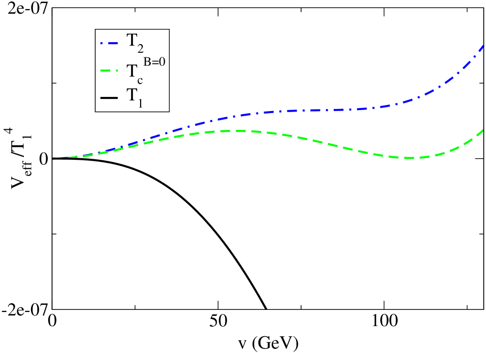
Figure 5: Finite temperature effective potential for the case $eB=0$ for three different temperatures. We use the values of the parameters $\mu=20$ GeV and $\lambda=0.0025$.

The complex fields $\phi$ and $\phi^{\dagger}$ can be equivalently expressed in terms of the two Hermitian fields $\sigma$ and $\chi$ by means of the definition

$$\phi(x) = \frac{1}{\sqrt{2}}[\sigma(x)+i\chi(x)]$$

$$\phi^{\dagger}(x) = \frac{1}{\sqrt{2}}[\sigma(x)-i\chi(x)]\,.$$ (67)

The Lagrangian in Eq. (64) is symmetric under the transformation $\phi\rightarrow-\phi$, however, the vacuum is not. Selecting the vacuum about which perturbative calculations can be performed, we shift the field by its classical value $v$ writing

$$\sigma\rightarrow v+\sigma\,.$$ (68)

After the shift, the mass of the fields $\sigma$ and $\chi$ become

$$m^{2}_{1}(v) = \frac{3}{4}\lambda v^{2}-\mu^{2}$$

$$m^{2}_{2}(v) = \frac{1}{4}\lambda v^{2}-\mu^{2}\,,$$ (69)

respectively. To lowest order (tree level) the potential is

$$V^{({\mbox{\tiny{tree}}})}=-\frac{1}{2}\mu^{2}v^{2}+\frac{1}{16}\lambda v^{4}\,.$$ (70)

To next order, we should include the zero-temperature part of the one-loop potential, given by

$$V^{(1)}_{\mbox{\tiny{vac}}}=\frac{1}{2}\int\frac{d^{3}k}{(2\pi)^{3}}\left(\sqrt{{\mathbf{k}}^{2}+m_{1}^{2}}+\sqrt{{\mathbf{k}}^{2}+m_{2}^{2}}\right)\,.$$ (71)

The integral in Eq. (71) is divergent and the theory must be renormalized. This can be achieved by introducing counter-terms in the Lagrangian of the form

$${\mathcal{L}}_{\mbox{\tiny{ct}}}=\frac{A}{2}v^{2}+\frac{B}{16}v^{4}+C\,,$$ (72)

where $C$ is a constant that can be used to cancel the $v$-independent part of the vacuum energy and $A$ and $B$ are determined by requiring that the infinities cancel. By this means, the effective potential up to one loop is Carrington

$$V_{\mbox{\tiny{vac}}}=-\frac{1}{2}\mu^{2}v^{2}+\frac{\lambda}{16}v^{4}+\frac{1}{32\pi^{2}}\sum_{i}m_{i}^{4}\ln(\frac{m_{i}}{2})\,,$$ (73)

where $m_{i}$, $i=1,2$ are given by Eqs. (69).

In the weak field limit, the finite-temperature effective potential, up to the contribution from the ring diagrams, is given by adding Eqs. (47) and (50) to Eq. (73), accounting for the contributions from the two fields $\sigma$ and $\chi$. Dropping the $v$-independent term, the result is

$$V(v)=-\frac{1}{2}\mu^{2}v^{2}+\frac{1}{16}\lambda v^{4}+\sum_{i}\left[\frac{m_{i}^{2}T^{2}}{24}-\frac{T}{12\pi}\left(m_{i}^{2}+\Pi_{1}\right)^{3/2}-\frac{(eB)^{2}}{4\pi}\left(\frac{\Pi_{1}}{48}\right)\left(\frac{T}{(m_{i}^{2}+\Pi_{1})^{3/2}}\right)+{\mathcal{O}}(m_{i}^{4})\right]$$ (74)

where $m_{i}$, $i=1,2$ are given by Eqs. (69) and $\Pi_{1}$ is given by Eq. (33). Notice that the terms proportional to $Tm_{i}^{3}$ and to $\ln(m_{i})$ have offset each other when adding up all the contributions. Also, in order for the terms involving the square root of the boson’s thermal mass to be real, the temperature must be such that

$$T>T_{1}\equiv\mu\sqrt{\frac{12}{\lambda}}\,,$$ (75)

which defines a lower bound for the temperature. Notice that the development of an imaginary part in the effective potential signals the onset of spinodal decomposition and the pase transition is quickly completed. This happens when the combination $m^{2}+\Pi_{1}$ becomes negative. For all values of $v$, this occurs for temperatures lower than $T_{1}$ defined in Eq. (75).

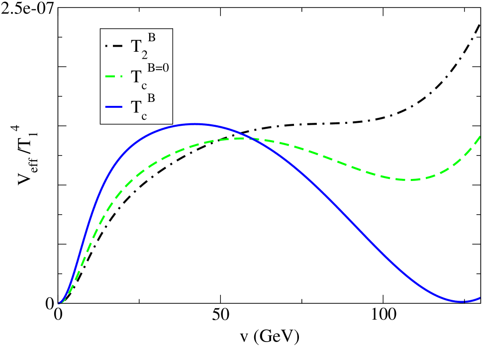
Figure 6: Finite temperature effective potential for the case $eB\neq 0$ for three different temperatures. We use the values of the parameters $\mu=20$ GeV, $\lambda=0.0025$ and $e=0.3$ and parametrize the magnetic field strength as $B=b(100)^{2}$ (GeV)², using $b=0.01$.

Figure 5 shows the finite temperature effective potential, discarding $v$-independent terms, for the case $B=0$ for three different temperatures, the above defined $T_{1}$, a temperature $T_{c}^{B=0}>T_{1}$ where the two minima coincide and a temperature $T_{2}>T_{c}^{B=0}$ where the second minimum of the potential disappears. For the calculation, we have used $\mu=20$ GeV and $\lambda=0.0025$.

Figure 6 shows the finite temperature effective potential, discarding $v$-independent terms, for the case $B\neq 0$ for the above defined temperature $T_{c}^{B=0}$ and two more values of the temperature: the curve with degenerate minima corresponds to a temperature $T_{c}^{B}<T_{c}^{B=0}$ and the curve where the second minimum has disappeared corresponds to a temperature $T_{2}^{B}>T_{c}^{B=0}$. For the calculation, we have used the same values of the parameters as for the case with $B=0$, taking $e=0.3$ and have parametrized the magnetic field strength as $B=b(100)^{2}$ (GeV)², using $b=0.01$.

Notice that the effect of the magnetic field is twofold: first it delays the starting of the phase transition down to a temperature $T_{c}^{B}<T_{c}^{B=0}$ and second, it makes the transition strongly first order. This second feature is best seen in Fig. 7 where we compare the effective potential obtained for $B=0$ and $B\neq 0$, discarding $v$-independent terms, for the two temperatures $T_{c}^{B=0}$ and $T_{c}^{B}$. For the latter temperature, the height of the barrier becomes larger signaling a stronger first order phase transition as compared to the case with $B=0$. The origin of this feature is that the corrections introduced by the magnetic field are inversely proportional to a power of the boson’s thermal mass and thus are larger for the value of $v$ when the mass parameters of Eqs. (69) vanish.

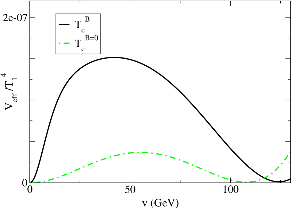
Figure 7: Comparison between the finite temperature effective potential for the cases with and without magnetic field evaluated at the temperatures where the minima of the potentials are degenerate. The height of the barrier between minima is higher in the case $eB\neq 0$, signaling a stronger first order phase transition. We use the values of the parameters $\mu=20$ GeV, $e=0.3$ and $\lambda=0.0025$ and parametrize the magnetic field strength as $B=b(100)^{2}$ (GeV)², using $b=0.01$.

V Conclusions

In this work we have studied the effects that the presence of a constant external magnetic field has on the effective potential for a charged scalar at finite temperature, up to the contribution from the ring diagrams. By studying symmetry restoration in the weak field limit we have found that the magnetic field is able to produce a stronger first order phase transition signaled by an increase in the height of the barrier between degenerate minima with respect to the case without magnetic field. The temperature for the onset of the phase transition is also lowered by the presence of the magnetic field as compared to the case without magnetic field.

The findings of this work show that there exists room in the parameter space of this theory where the effects of the magnetic field could be important. In particular, an extension of these ideas to the case of the SM degrees of freedom to describe the EWPT could be significant for the problem of the generation of baryon number. This is work under progress and will be reported as a sequel of the present one.

Appendix

We start first by evaluating the integrals

$$J_{1} = T\sum_{n}\int\frac{d^{3}k}{(2\pi)^{3}}\frac{1}{(\omega_{n}^{2}+{\mathbf{k}}^{2}+m^{2})^{2}}$$

$$J_{2} = \left(\frac{4}{3}\right)T\sum_{n}\int\frac{d^{3}k}{(2\pi)^{3}}\frac{\mathbf{k}^{2}}{(\omega_{n}^{2}+{\mathbf{k}}^{2}+m^{2})^{3}}\,,$$ (76)

appearing in the computation of the effective potential in the weak field limit, Eq. (46). To this end, notice that we can write

$$J_{1} = T\sum_{n}\int\frac{d^{3}k}{(2\pi)^{3}}f({\mathbf{k}}^{2})$$

$$J_{2} = -\left(\frac{1}{3}\right)T\sum_{n}\int\frac{d^{3}k}{(2\pi)^{3}}{\mathbf{k}}\cdot{\mathbf{\nabla}}_{k}f({\mathbf{k}}^{2})\,,$$ (77)

where

$$f({\mathbf{k}}^{2})=\frac{1}{(\omega_{n}^{2}+{\mathbf{k}}^{2}+m^{2})^{2}}\,.$$ (78)

Integrating by parts the second of Eqs. (77) we get

$$J_{2} = -\left(\frac{1}{3}\right)T\sum_{n}\int\frac{d^{3}k}{(2\pi)^{3}}{\mathbf{\nabla}}_{k}\cdot\left({\mathbf{k}}f({\mathbf{k}}^{2})\right)$$ (79)

$$+ \left(\frac{1}{3}\right)T\sum_{n}\int\frac{d^{3}k}{(2\pi)^{3}}f({\mathbf{k}}^{2}){\mathbf{\nabla}}_{k}\cdot{\mathbf{k}}\,.$$

The first of the terms in Eq. (79) can be converted into a surface integral and since $f({\mathbf{k}}^{2})$ decreases faster than ${\mathbf{k}}^{-2}$ at infinity, this surface term vanishes. Also, using that ${\mathbf{\nabla}}_{k}\cdot{\mathbf{k}}=3$, we finally get $J_{1}=J_{2}$.

References

- (1) For comprehensive reviews on the dynamics of the EWPT see for example A. Megevand, Int. J. Mod. Phys. D9, 733 (2000); N. Petropoulos, “Baryogenesis at the electroweak phase transition”, hep-ph/0304275.
- (2) K. Enqvist, Int. J. Mod. Phys. D7, 331 (1998); R. Maartens, “Cosmological magnetic fields”, International Conference on Gravitation and Cosmology, India, Jan. 2000, Pramana 55, 575 (2000); D. Grasso and H.R. Rubinstein, Phys. Rep. 348 163, (2001); M. Giovannini, Int. J. Mod. Phys. D13, 391-502 (2004).
- (3) A. Ayala, J. Besprosvany, G. Pallares and G. Piccinelli, Phys. Rev. D64, 123529 (2001); A. Ayala, G. Piccinelli and G. Pallares, Phys. Rev. D66, 103503 (2002), A. Ayala and J. Besprosvany, Nucl. Phys. B651, 211 (2004).
- (4) L. Campanelli, G.L. Fogli and L. Tedesco, Phys. Rev. D 70, 083502 (2004).
- (5) M. Giovannini and M. E. Shaposhnikov, Phys. Rev. D57, 2186 (1998).
- (6) P. Elmfors, K. Enqvist and K. Kainulainen, Phys. Lett. B 440, 269 (1998).
- (7) M. Giovannini, Phys. Rev. D61, 063004 (2000).
- (8) K. Kajantie, M. Laine, J. Peisa, K. Rummukainen and M. Shaposhnikov, Nucl. Phys. B 544, 357 (1999).
- (9) V. Skalozub and M. Bordag, Int. J. Mod. Phys. A 15, 349 (2000).
- (10) J. Schwinger, Phys. Rev. 82, 664 (1951).
- (11) J.C. D’Olivo, J.F. Nieves, S. Sahu, Phys. Rev. D 67, 025018 (2003).
- (12) T.-K. Chyi, C.-W. Hwang, W.F. Kao, G.L. Lin, K.-W. Ng and J.-J. Tseng, Phys. Rev. D 62, 105014, (2000).
- (13) M. Le Bellac Thermal Field Theory, Cambridge University Press (1996).
- (14) M.E. Carrington, Phys. Rev. D45, 2933 (1992).
- (15) D.J. Bedingham, “Dimensional regularization and Mellin summation in high temperature calculations”, hep-ph/0011012.
- (16) L. Dolan and R. Jackiw, Phys. Rev. D9, 3320 (1974).