PCCF RI 0417

${\rm ECT}^{*}$-04-22

$\boldsymbol{\Lambda_{b}}$ Decays into $\boldsymbol{\Lambda}$-Vector

Z.J. Ajaltouni¹, E. Conte², O. Leitner^3
1,2 Laboratoire de Physique Corpusculaire de Clermont-Ferrand

IN2P3/CNRS Université Blaise Pascal

F-63177 Aubière Cedex France

³ ${\rm{ECT}}^{*}$, Strada delle Tabarelle, 286, 38050 Villazzano (Trento), Italy

A complete study of the angular distributions of the processes, $\Lambda_{b}\to{\Lambda}V(1^{-})$, with $\Lambda\to p{\pi}^{-}$ and $V(J/{\Psi})\to{\ell}^{+}{\ell}^{-}$ or $V({\rho}^{0},\omega)\to{\pi}^{+}{\pi}^{-},$ is performed. Emphasis is put on the initial $\Lambda_{b}$ polarization produced in the proton-proton collisions. The polarization density-matrices as well as angular distributions are derived and help to construct T-odd observables which allow us to perform tests of both Time-Reversal and $CP$ violation.

PACS Numbers: 11.30.Er, 12.39.-x, 13.30.-a, 14.20.-c, 14.20.Mr
Keywords: Helicity, baryon decay, polarization

1 Introduction

With the advent of $B$-factories at the proton-proton colliders, huge statistics of beauty hadrons are expected to be produced. This will allow a thorough study of $CP$ violation processes with $B$ mesons. Moreover, some specific phenomena related to either $b$-quark physics or $CP$ violation can be performed to put limits on the validity of the Standard Model (SM). One of these processes concerns the validity of the Time Reversal (TR) symmetry. A promising method to look for TR violation is the three body $\Lambda_{b}$ decay [1, 2] as it was initiated with the hyperons long time ago by R. Gatto [3].

T-odd operator is derived from Time Reversal and it keeps the initial and final states unchanged. It is well known that the time reversing state of a decay like $\Lambda\to p{\pi}^{-}$ or $\beta$ nucleon decay cannot be realized in the physical world, thus we must be contented with the following transformations which are the main ingredients of TR operator:

$$\vec{r}\xrightarrow{T}\vec{r}\ ,\;\;\vec{p}\xrightarrow{T}-{\vec{p}}\ ,\;\;\vec{\ell}\xrightarrow{T}-{\vec{\ell}}\ ,\;\;\vec{s}\xrightarrow{T}-{\vec{s}}\ ,$$

where $\vec{\ell}$ and $\vec{s}$ are respectively the angular momentum and the spin of any particle with momentum $\vec{p}$. Consequently the helicity of the particle defined by $\lambda={\vec{s}}\cdot{\vec{p}}/p$ remains unchanged by TR transformations.

In the past, it was pointed out by many authors [4] the importance to look for T-odd effects in the hyperon decays like $\Lambda,\Sigma$ and $\Xi$, as being a consequence of both $CPT$ theorem and $CP$ violation in weak $|{\Delta}S|=1$ decays. As far as beauty hadrons ${\Lambda}_{b},{\Sigma}_{b}$ and ${\Xi}_{b}$ are concerned, because of their numerous decay channels and the strength of $CP$ violation in the $b$-quark sector, opportunities to find T-odd observables will increase and interesting tests of both the SM and models beyond the SM can be performed successfully. Due to the initial polarization of the $\Lambda_{b}$ baryon, T-odd observables can be constructed from the decay products such as $\vec{v_{1}}\cdot{(\vec{v_{2}}\times\vec{v_{3}})}$ where $\vec{v_{i}}$ is either the spin or the momentum of the particle $i$. These observables change sign under TR transformations and a non-vanishing mean value of their distribution could be a sign of TR violation.

This paper is devoted to a study and simulations of $\Lambda_{b}$ decays into $\Lambda{\ell}^{+}{\ell}^{-}$ and $\Lambda h^{+}h^{-}$. Final leptons, $\ell=e,\mu$, or final hadron, $h=\pi$, can originate from intermediate resonances which quantum numbers are those of a vector meson $1^{-}$ like $J/\psi,{\rho}^{0}$ and $\omega$. The reminder of this paper is organized as it follows. In section 2, we present an analysis of both the intermediate states and the final particles in some appropriate frames, the helicity frames. By stressing on the importance of the polarizations of the initial $\Lambda_{b}$ as well as the intermediate resonances, calculations based on the helicity formalism are performed and take into account the spin properties of the final decay products. Dynamical assumption is made through the factorization framework applied in baryon decays in section 3. The following section is devoted to results and discussions for angular distributions and polarization density matrices. Finally, in the last section, we draw some conclusions.

2 $\boldsymbol{\Lambda_{b}}$ decay analysis

In the collisions, $pp\rightarrow{\Lambda_{b}}+X$, the $\Lambda_{b}$ is produced with a transverse polarization in a similar way than the ordinary hyperons. Its longitudinal polarization is suppressed because of parity conservation in strong interactions. Let us define, ${\vec{N}}_{P}$, the vector normal to the production plane by:

$${\vec{N}}_{P}=\frac{\vec{p}_{1}\times\vec{p}_{b}}{|{\vec{p}_{1}\times\vec{p}_{b}}|}\ ,$$ (1)

where $\vec{p}_{1}$ and $\vec{p}_{b}$ are the vector-momenta of one incident proton beam and $\Lambda_{b}$, respectively. The mean value of the $\Lambda_{b}$ spin along ${\vec{N}}_{P}$ is the $\Lambda_{b}$ transverse polarization usually greater than $20\%$ [5].

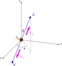
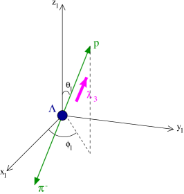
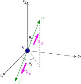
Figure 1: Left-handed: $\Lambda_{b}$ decay in its transversity frame. Right-handed: helicity frames for the $\Lambda$ and vector meson V decays, respectively.

Let $({\Lambda_{b}}xyz)$ be the rest frame (see Fig. 1) of the $\Lambda_{b}$ particle. The quantization axis $({\Lambda_{b}}z)$ is chosen to be parallel to ${\vec{N}}_{P}$. The other orthogonal axis $({\Lambda_{b}}x)$ and $({\Lambda_{b}}y)$ are chosen arbitrarily in the production plane. In our analysis, the $({\Lambda_{b}}x)$ axis is taken parallel to the momentum $\vec{p}_{1}$. The spin projection, $M_{i}$, of the $\Lambda_{b}$ along the transverse axis $({\Lambda_{b}}z)$ takes the values $\pm{1/2}$. The polarization density matrix, ${\rho}^{\Lambda_{b}}$, of the $\Lambda_{b}$ is a $(2\times 2)$ hermitian matrix. Its elements, ${\rho}_{ii}^{\Lambda_{b}}$, are real and $\sum_{i=1}^{2}{\rho}_{ii}^{\Lambda_{b}}=1$. The probability of having $\Lambda_{b}$ produced with $M_{i}=\pm{1/2}$ is given by ${\rho}_{11}^{\Lambda_{b}}$ and ${\rho}_{22}^{\Lambda_{b}}$, respectively. Finally, the initial $\Lambda_{b}$ polarization, ${\cal P}_{\Lambda_{b}}$, is given by $\langle\vec{S}_{\Lambda_{b}}\cdot\vec{N}_{P}\rangle={\cal P}_{\Lambda_{b}}={\rho}_{11}^{\Lambda_{b}}-{\rho}_{22}^{\Lambda_{b}}.$

The decay amplitude, $A_{0}{(M_{i})}$, for ${\Lambda_{b}}{(M_{i})}\to{\Lambda}{(\lambda_{1})}V{(\lambda_{2})}$ is obtained by applying the Wigner-Eckart theorem to the $S$-matrix element in the framework of the Jacob-Wick helicity formalism [6]:

$$A_{0}{(M_{i})}=\langle 1/2,M_{i}|S^{(0)}|p,\theta,\phi;\lambda_{1},\lambda_{2}\rangle=\mathcal{M}_{\Lambda_{b}}{(\lambda_{1},\lambda_{2})}D_{M_{i}M_{f}}^{{1/2}\star}{(\phi,\theta,0)}\ ,$$ (2)

where $\vec{p}=(p,\theta,\phi)$ is the vector-momentum of the hyperon $\Lambda$ in the $\Lambda_{b}$ frame (Fig. 1). $\lambda_{1}$ and $\lambda_{2}$ are the respective helicities of $\Lambda$ and $V$ with the possible values $\lambda_{1}=\pm{1/2}$ and $\lambda_{2}=-1,0,+1$. The momentum projection along the $({\Delta})$ axis (parallel to $\vec{p}$) is given by $M_{f}=\lambda_{1}-\lambda_{2}=\pm{1/2}$. The $M_{f}$ values constrain those of $\lambda_{1}$ and $\lambda_{2}$ since, among six combinations, only four are physical. If $M_{f}=+1/2$ then $(\lambda_{1},\lambda_{2})=(1/2,0)$ or $(-1/2,-1)$. If $M_{f}=-1/2$ then $(\lambda_{1},\lambda_{2})=(1/2,1)$ or $(-1/2,0)$. The hadronic matrix element, $\mathcal{M}_{\Lambda_{b}}{(\lambda_{1},\lambda_{2})}$, contains all the decay dynamics. Finally, the Wigner matrix element,

$$D_{M_{i}M_{f}}^{j}{(\phi,\theta,0)}=d_{M_{i}M_{f}}^{j}{(\theta)}{\exp{(-i{M_{i}}{\phi})}}\ ,$$ (3)

is expressed according to the Jackson convention [6].

In case of two intermediate resonances such as those described in the next section, the $\Lambda_{b}$-decay plane is defined by the momenta of the $\Lambda$ and leptons (or hadrons). This decay plane does not coincide with that one defined by the momenta of the $J/\Psi$, proton and pion.

2.1 Decay of the intermediate resonances

By performing appropriate rotations and Lorentz boosts, we can study the decay of each resonance in its own helicity frame (see Fig. 1) such that the quantization axis is parallel to the resonance momentum in the $\Lambda_{b}$ frame i.e. $\overrightarrow{O_{1}z_{1}}||\vec{p}_{\Lambda}$ and $\overrightarrow{O_{2}z_{2}}||\vec{p}_{V}=-\vec{p}_{\Lambda}$. For the decays ${\Lambda}{(\lambda_{1})}\to P{(\lambda_{3})}{\pi}^{-}{(\lambda_{4})}$ and $V{(\lambda_{2})}\to{\ell}^{-}{(\lambda_{5})}{\ell}^{+}{(\lambda_{6})}$ or $V{(\lambda_{2})}\to h^{-}{(\lambda_{5})}h^{+}{(\lambda_{6})},$ the respective helicities of the final particles are $(\lambda_{3},\lambda_{4})=(\pm{1/2},0)$ and $(\lambda_{5},\lambda_{6})=(\pm{1/2},\pm{1/2})$ in case of leptons or $(\lambda_{5},\lambda_{6})=(0,0)$ in case of $0^{-}$ mesons.

In the $\Lambda$ helicity frame, the projection of the total angular momentum, $m_{i}$, along the proton momentum, $\vec{p}_{P}$, is given by $m_{1}=\lambda_{3}-\lambda_{4}=\pm{1/2}$. In the vector meson helicity frame, this projection is equal to $m_{2}=\lambda_{5}-\lambda_{6}=-1,0,+1$ if leptons and $m_{2}=0$ if $\pi$. The decay amplitude, $A_{i}(\lambda_{i})$, of each resonance can be written similarly as in Eq. (2), requiring only that the kinematics of its decay products are fixed. We obtain,

$$A_{1}(\lambda_{1})=\langle\lambda_{1},m_{1}|S^{(1)}|p_{1},{\theta}_{1},{\phi}_{1};\lambda_{3},\lambda_{4}\rangle=\mathcal{M}_{\Lambda}{(\lambda_{3},\lambda_{4})}D^{{1/2}\star}_{\lambda_{1}m_{1}}{(\phi_{1},\theta_{1},0)}\ ,$$

$$A_{2}(\lambda_{2})=\langle\lambda_{2},m_{2}|S^{(2)}|p_{2},{\theta}_{2},{\phi}_{2};\lambda_{5},\lambda_{6}\rangle=\mathcal{M}_{V}{(\lambda_{5},\lambda_{6})}D^{1\star}_{\lambda_{2}m_{2}}{(\phi_{2},\theta_{2},0)}\ ,$$ (4)

where $\theta_{1}$ and $\phi_{1}$ are respectively the polar and azimuthal angles of the proton momentum in the $\Lambda$ rest frame while $\theta_{2}$ and $\phi_{2}$ are those of ${\ell}^{-}{(h^{-})}$ in the $V$ rest frame.

2.2 Analytical form of the decay probability

The general decay amplitude, ${\cal A}_{I}$, for the process, $\Lambda_{b}{(M_{i})}\to\Lambda{(\lambda_{1})}V{(\lambda_{2})}\Longrightarrow P{\pi}^{-}\;{\ell}^{+}{\ell}^{-}$, must include all the possible intermediate states so that a sum over the helicity states ${(\lambda_{1},\lambda_{2})}$ is performed:

$${\cal A}_{I}=\sum_{\lambda_{1},\lambda_{2}}{A_{0}{(M_{i})}A_{1}{(\lambda_{1})}A_{2}{(\lambda_{2})}}\ .$$ (5)

The decay probability, $d\sigma$, depending on the amplitude, ${\cal A}_{I}$, takes the form,

$$d\sigma\propto\sum_{M_{i},M^{\prime}_{i}}{\rho}_{M_{i}M^{\prime}_{i}}^{\Lambda_{b}}{\cal A}_{I}{\cal A}_{I}^{*}\ ,$$ (6)

where the polarization density matrix, ${\rho}_{M_{i}M^{\prime}_{i}}^{\Lambda_{b}}$, is used to take into account the unknown $\Lambda_{b}$ spin component, $M_{i}$. Since the helicities of the final particles are not measured, a summation over the helicity values $\lambda_{3},\lambda_{4},\lambda_{5}$ and $\lambda_{6}$ is performed as well. Finally, the decay probability, $d\sigma$, written in a such way that only the intermediate resonance helicities appear, reads as,

$$d\sigma\propto\sum_{\lambda_{1},\lambda_{2},{\lambda}^{\prime}_{1},{\lambda}^{\prime}_{2}}D_{\lambda_{1}-\lambda_{2},{\lambda}^{\prime}_{1}-{\lambda}^{\prime}_{2}}{(\theta,\phi,0)}{\rho}_{\lambda_{1}-\lambda_{2},{\lambda}^{\prime}_{1}-{\lambda}^{\prime}_{2}}^{\Lambda_{b}}{\mathcal{M}_{\Lambda_{b}}{(\lambda_{1},\lambda_{2})}}\\ \mathcal{M}_{\Lambda_{b}}^{*}{({\lambda}^{\prime}_{1},{\lambda}^{\prime}_{2})}F^{\Lambda}_{\lambda_{1}{\lambda}^{\prime}_{1}}{(\theta_{1},\phi_{1})}G^{V}_{\lambda_{2}{\lambda}^{\prime}_{2}}{(\theta_{2},\phi_{2})}\ ,$$ (7)

where $F^{\Lambda}_{\lambda_{1}{\lambda}^{\prime}_{1}}{(\theta_{1},\phi_{1})}$ and $G^{V}_{\lambda_{2}{\lambda}^{\prime}_{2}}{(\theta_{2},\phi_{2})}$ describing the decay dynamics of the intermediate resonances $\Lambda\to P{\pi}^{-}$ and $V\to{\ell}^{+}{\ell}^{-}$, respectively, are given in Appendix. Because of parity violation in weak hadronic decays, it is assumed that $\mathcal{M}_{\Lambda_{b}}{(\lambda_{1},\lambda_{2})}$ is not equal to $\mathcal{M}_{\Lambda_{b}}{(-\lambda_{1},-\lambda_{2})}$.

3 Factorization procedure

In tree approximation, the effective interaction, $\mathcal{H}^{eff}$, written as,

$$\mathcal{H}^{eff}=\frac{G_{F}}{\sqrt{2}}V_{qb}V^{\star}_{qs}\sum_{i=1}^{2}c_{i}(m_{b})O_{i}(m_{b})\ ,$$ (8)

gives the weak following amplitude factorized into,

$$\mathcal{M}_{\Lambda_{b}}(\Lambda_{b}\to\Lambda V)=\frac{G_{F}}{\sqrt{2}}V_{qb}V^{\star}_{qs}f_{V}E_{V}\Bigl{(}c_{1}+\frac{c_{2}}{N_{c}^{eff}}\Bigr{)}\langle\Lambda|\bar{s}\gamma_{\mu}(1-\gamma_{5})b|\Lambda_{b}\rangle\ .$$ (9)

The CKM matrix elements, $V_{qb}V^{\star}_{qs}$, read as $V_{ub}V^{\star}_{us}$ and $V_{cb}V^{\star}_{cs}$, in case of $\Lambda_{b}\to\Lambda\rho$ and $\Lambda_{b}\to\Lambda J/\Psi$, respectively. The Wilson Coefficients, $c_{i}$, are equal to $c_{1}=-0.3$ and $c_{2}=+1.15$. The hadronic matrix element, $\langle\Lambda|\bar{s}\gamma_{\mu}(1-\gamma_{5})b|\Lambda_{b}\rangle$, can be derived respecting Lorentz decomposition. Working in HQET, it is more convenient to use [7],

$$\langle\Lambda|\bar{s}\gamma_{\mu}(1-\gamma_{5})b|\Lambda_{b}\rangle=\bar{u}_{\Lambda}\Bigl{[}\bigl{\{}F_{1}(q^{2})+/\!\!\!vF_{2}(q^{2})\bigr{\}}\gamma_{\mu}(1-\gamma_{5})\Bigr{]}u_{\Lambda_{b}}\ ,$$ (10)

where the four-velocity of $\Lambda_{b}$ is $v=P_{\Lambda_{b}}/M_{\Lambda_{b}}$. The momentum transfer is denoted by $q=P_{\Lambda_{b}}-P_{\Lambda}$ and $F_{i}(q^{2})$ are the form factors involved in the transition $\Lambda_{b}\to\Lambda$. The final amplitude, $\mathcal{M}_{\Lambda_{b}}(\Lambda_{b}\to\Lambda V)$, depending on the helicity state, $(\lambda_{\Lambda},\lambda_{V})$, reads as,

$$\mathcal{M}_{\Lambda_{b}}(\Lambda_{b}\to\Lambda V)=\left\{\,\,\begin{array}[]{ll}{\displaystyle-\frac{P_{V}}{E_{V}}\Biggl{(}\frac{m_{\Lambda_{b}}+m_{\Lambda}}{E_{\Lambda}+m_{\Lambda}}F^{-}(q^{2})+2F_{2}(q^{2})\Biggl{)}}\,;&(\lambda_{\Lambda},\lambda_{V})=(\frac{1}{2},0)\ ,\\[11.38092pt] {\displaystyle\frac{1}{\sqrt{2}}\Biggl{(}\frac{P_{V}}{E_{\Lambda}+m_{\Lambda}}F^{-}(q^{2})+F^{+}(q^{2})\Biggl{)}}\,;&(\lambda_{\Lambda},\lambda_{V})=(-\frac{1}{2},-1)\ ,\\[11.38092pt] {\displaystyle\frac{1}{\sqrt{2}}\Biggl{(}\frac{P_{V}}{E_{\Lambda}+m_{\Lambda}}F^{-}(q^{2})-F^{+}(q^{2})\Biggl{)}}\,;&(\lambda_{\Lambda},\lambda_{V})=(\frac{1}{2},1)\ ,\\[11.38092pt] {\displaystyle\Biggl{(}F^{+}(q^{2})+\frac{P^{2}_{V}}{E_{V}(E_{V}+m_{\Lambda})}F^{-}(q^{2})\Biggl{)}}\,;&(\lambda_{\Lambda},\lambda_{V})=(-\frac{1}{2},0)\ .\\[11.38092pt] \end{array}\right.$$ (11)

The $q^{2}$ dependence of the transition form factors, $F_{i}(q^{2})$, or $(F^{\pm}(q^{2}))$, resulting from QCD sum rules and HQET [8] takes the form as it follows,

$$F_{i}(q^{2})=\frac{F(0)}{1-a\frac{q^{2}}{m^{2}_{\Lambda_{b}}}+b\frac{q^{4}}{m^{4}_{\Lambda_{b}}}}\ ,$$ (12)

where the following values $(0.462,-0.0182,-1.76\!\times\!10^{-4})$ and $(-0.077,-0.0685,1.46\!\times\!10^{-3})$ correspond to $(F(0),a,b)$ in case of $F_{1}(q^{2})$ and $F_{2}(q^{2})$, respectively. We refer to the PDG [9] for all the numerical values used in our analysis.

4 Results

Departing from the previous relations, physical observables like the helicity asymmetry parameter, $\alpha_{As}^{\Lambda_{b}}$, the polarization density matrices, $\rho^{V,\Lambda}$, and the branching ratios, $\mathcal{BR}({\Lambda}_{b}\to{\Lambda}{\rho}^{0})$ and $\mathcal{BR}({\Lambda}_{b}\to{\Lambda}J/\Psi)$, can be evaluated.

Owing to the spin $1/2$ of the $\Lambda_{b}$, the angular momentum projection along the helicity axis (which direction is given by the $\Lambda$ vector-momentum) has only two values, $M_{i}=\pm 1/2$, with respective weights generally different. The helicity asymmetry parameter, $\alpha_{As}^{\Lambda_{b}}$, defined in Eq. (14), takes the following values:

$${\alpha}^{\Lambda_{b}}_{AS}=98.8\% \;\;{\rm for}\;\;\Lambda_{b}\to\Lambda\rho^{0}\ ,$$

$${\alpha}^{\Lambda_{b}}_{AS}=77.7\% \;\;{\rm for}\;\;\Lambda_{b}\to\Lambda J/\Psi\ .$$

From these results, the angular momentum projection, $M_{i}=1/2$, appears to be largely dominant in the analyzed decays.

The $\Lambda$-polarization, $\mathcal{P}_{\Lambda}=\rho_{ii}^{\Lambda}-\rho_{jj}^{\Lambda}$, with $\rho_{ii}^{\Lambda}$ defined in Eq. (17), can be computed in both decay cases. After normalization of $\mathcal{P}_{\Lambda}$, we obtain the values, $\mathcal{P}_{\Lambda}=+31\%$, and $\mathcal{P}_{\Lambda}=-9\%$, for $\Lambda_{b}\to\Lambda{\rho}^{0}$ and $\Lambda_{b}\to\Lambda J/{\psi}$, respectively. The other important parameter concerning the spin state of the intermediate resonances is the density matrix element, $\rho^{V}_{ij}$, defined in Eq. (20). Let us focus on the matrix element, $\rho^{V}_{00}$, which is related to the longitudinal polarization of the vector meson V. After calculation, $65.5\%$ and $55.5\%$ are the results for the density matrix element, $\rho^{V}_{00},$ in case of $\Lambda_{b}\to\Lambda{\rho}^{0}$ and $\Lambda_{b}\to\Lambda J/{\psi}$, respectively. It is important to notice that these parameters, ${\alpha}^{\Lambda_{b}}_{AS}$ and $\rho^{V}_{ij},$ (as well as $\rho^{\Lambda}_{ij}$) govern entirely the angular distributions, $W_{i}(\theta_{i},\phi_{i})$, of the final particles in each resonance frame.

In Fig. 2, are shown the polar angular distributions (which do not depend on $\Lambda_{b}$ initial polarization) for proton and $l(h)$ coming respectively from $\Lambda$ and V decays. In the same figure, the transverse momentum distributions, $P_{\perp}^{P}$ and $P_{\perp}^{\pi}$ ($\Lambda$ daughters) given in the $\Lambda_{b}$ rest frame, are plotted. These distributions look to be discriminant in the investigation of $\Lambda_{b}$ decay observables.

Finally, the last step is the computation of the branching ratios, $\mathcal{BR}(\Lambda_{b}\to\Lambda{\rho}^{0})$ and $\mathcal{BR}(\Lambda_{b}\to\Lambda J/{\psi})$, which requires the calculation of their corresponding widths. The standard expression of a decay width, $\Gamma(\Lambda_{b}\to\Lambda V)$, is given by,

$$\Gamma(\Lambda_{b}\to\Lambda V)=\frac{E_{\Lambda}+M_{\Lambda}}{M_{\Lambda_{b}}}\frac{P_{V}}{16\pi^{2}}\int_{\Omega}|A_{0}(M_{i})|^{2}d\Omega\ ,$$

where $E_{\Lambda}$ and $P_{V}$ are respectively the energy and momentum of the $\Lambda$ baryon and vector meson in the $\Lambda_{b}$ rest frame. $\Omega$ corresponds to the decay solid angle. Performing all the calculations and keeping the number of color, $N_{c}^{eff}$, to vary between the values 2 and 3 as it is suggested by the factorization hypothesis, we obtain the following branching ratio results:

$$\mathcal{BR}(\Lambda_{b}\to\Lambda\rho^{0})= (34.0\ ,11.4\ ,3.1)\times 10^{-8}\ ,$$

$$\mathcal{BR}(\Lambda_{b}\to\Lambda J/\psi)= (12.5\ ,4.4\ ,1.2)\times 10^{-4}\ ,$$

respectively for $N_{c}^{eff}=2,2.5$ and $3$. These interesting results suggest that the effective number of color might be taken greater than $2.5$ in the framework of the factorization hypothesis in case of $\Lambda_{b}$ decay. It is worth comparing the theoretical branching ratio, $\mathcal{BR}^{th}(\Lambda_{b}\to\Lambda J/\psi)$, with the experimental one [9], $\mathcal{BR}^{exp}(\Lambda_{b}\to\Lambda J/\psi)=(4.7\pm 2.1\pm 1.9)\times 10^{-4}$.

5 Conclusion

Calculations of the angular distributions as well as branching ratios of the process $\Lambda_{b}\to\Lambda V$ with $\Lambda\to P{\pi}^{-}$ and $V\to{\ell}^{+}{\ell}^{-}$ or $V\to h^{+}h^{-}$ have been performed by using the helicity formalism and stressing on the correlations which arise among the final decay products. In all these calculations, particular role of the $\Lambda_{b}$ polarization has been put into evidence. The initial polarization, ${\cal P}_{\Lambda_{b}}$, appears explicitly in the polar angle distribution of the $\Lambda$ hyperon in the $\Lambda_{b}$ rest-frame. Similarly, the azimuthal angle distributions of both proton and ${\ell}^{-}$ in the $\Lambda$ and $V$ frames, respectively, depend directly on the $\Lambda_{b}$ polarization. Furthermore, a first computation of the asymmetry parameter, ${\alpha}_{As}$, in $\Lambda_{b}$ decays into $\Lambda V(1^{-})$ has been performed as well as the longitudinal polarization of the vector meson, ${\rho}_{00}^{V}$, which is shown to be dominant $(\geq 56\%)$.

On the other hand, it is well known that the violation of $CP$ symmetry via the CKM mechanism is one of the corner-stone of the Standard Model of particle physics. Looking for TR violation effects in baryon decays provides us a new field of research: firstly as a complementary test of $CP$ violation by assuming the correctness of the $CPT$ theorem and, secondly, as a possibility to search for processes beyond the Standard Model. In particular, triple product correlations, which are $T$-odd under time reversal, can be extensively investigated in $\Lambda_{b}$ decays. However, this latter aim requires both experimental and theoretical improvements in order to increase our knowledge of $b$-physics.

Acknowledgments

The authors are indebted to their colleagues of the LHCB Clermont-Ferrand team for internal discussions regarding this promising research subject of Time Reversal.

Appendix

Appendix A Angular distributions

A.1 $\boldsymbol{\Lambda_{b}\to\Lambda V}$ decay

Writing the hadronic matrix element, $\mathcal{M}_{\Lambda_{b}}(\lambda_{1},\lambda_{2})$, into two parameters according to the final helicity value such as,

$${|\mathcal{M}_{\Lambda_{b}}(\pm 1/2)|}^{2}=\ {|\mathcal{M}_{\Lambda_{b}}(\pm 1/2,0)|}^{2}+{|\mathcal{M}_{\Lambda_{b}}(\mp 1/2,\mp 1)|}^{2}\ ,$$ (13)

and by introducing the helicity asymmetry parameter, ${\alpha}_{As}^{\Lambda_{b}}$, defined by,

$$\alpha_{AS}^{\Lambda_{b}}=\frac{{|\mathcal{M}_{\Lambda_{b}}{(+1/2)}|}^{2}-{|\mathcal{M}_{\Lambda_{b}}{(-1/2)}|}^{2}}{{|\mathcal{M}_{\Lambda_{b}}{(+1/2)}|}^{2}+{|\mathcal{M}_{\Lambda_{b}}{(-1/2)}|}^{2}}\ ,$$ (14)

the final angular distribution, $W{(\theta,\phi)}$, deduced from Eq. (7) and expressed as

$$W{(\theta,\phi)}\propto 1+{\alpha_{AS}^{\Lambda_{b}}}{\cal P}_{\Lambda_{b}}{\cos\theta}+2{\alpha_{AS}^{\Lambda_{b}}}\Re e\Big{[}{\rho}_{ij}^{\Lambda_{b}}{\exp{(-i\phi)}}\Big{]}\sin{\theta}\ ,$$ (15)

puts into evidence the parity violation.

A.2 $\boldsymbol{\Lambda\to P{\pi}^{-}}$ decay

From Eq. (7), integrating over the angles $\theta,\phi,\theta_{2}$ and $\phi_{2}$ and summing over vector helicity states, the general formula for proton angular distributions, $W_{1}{(\theta_{1},\phi_{1})}$, in the $\Lambda$ frame reads as,

$$W_{1}{(\theta_{1},\phi_{1})}\propto\\ \frac{1}{2}\Biggl{\{}({\rho}_{ii}^{\Lambda}+{\rho}_{jj}^{\Lambda})+({\rho}_{ii}^{\Lambda}-{\rho}_{jj}^{\Lambda})\alpha_{AS}^{\Lambda}\cos\theta_{1}-\frac{\pi}{2}{\cal P}_{\Lambda_{b}}\alpha_{AS}^{\Lambda}\Re e\Big{[}{\rho}_{ij}^{\Lambda}\exp{(i\phi_{1})}\Big{]}\sin{\theta_{1}}\Biggr{\}}\ ,$$ (16)

where the PDM elements, ${\rho}_{ij}^{\Lambda}$, of the baryon $\Lambda$ are (to a normalization factor):

$${\rho}^{\Lambda}_{ii} ={\int_{\theta_{2},\phi_{2}}}G^{V}_{00}{(\theta_{2},\phi_{2})}\ {|\mathcal{M}_{\Lambda_{b}}{(\pm 1/2,0)}|}^{2}+{\int_{\theta_{2},\phi_{2}}}G^{V}_{\pm 1\pm 1}{(\theta_{2},\phi_{2})}{|\mathcal{M}_{\Lambda_{b}}{(\pm 1/2,\pm 1)}|}^{2}\ ,$$

$${\rho}^{\Lambda}_{ij} ={\int_{\theta_{2},\phi_{2}}}{G^{V}_{00}}{(\theta_{2},\phi_{2})}\mathcal{M}_{\Lambda_{b}}{(-1/2,0)}\mathcal{M}_{\Lambda_{b}}^{*}{(1/2,0)}\ .$$ (17)

The hermitian matrix, $G^{V}_{\lambda_{2}{\lambda}^{\prime}_{2}}{(\theta_{2},\phi_{2})}$, describing the process, $V\to{\ell}^{+}{\ell}^{-}$ or $V\to h^{+}h^{-}$, has the following form:

$$G^{V}_{\lambda_{2}{\lambda}^{\prime}_{2}}{(\theta_{2},\phi_{2})}=\sum_{\lambda_{5},\lambda_{6}}{|\mathcal{M}_{V}(\lambda_{5},\lambda_{6})|}^{2}d^{1}_{\lambda_{2}m_{2}}{(\theta_{2})}d^{1}_{{\lambda}^{\prime}_{2}m_{2}}{(\theta_{2})}\exp{i(\lambda_{2}-{\lambda}^{\prime}_{2})\phi_{2}}\ ,$$ (18)

with $m_{2}=\lambda_{5}-\lambda_{6}$. In case of lepton pair in the final state, because of parity conservation, two hadronic matrix elements, $\mathcal{M}_{V}(\frac{1}{2},\pm\frac{1}{2})$, are necessary whereas only one, $\mathcal{M}_{V}(0,0)$, is required in case of pseudo-scalar mesons.

A.3 $\boldsymbol{V\to{\ell}^{+}{\ell}^{-}(h^{+}h^{-})}$

Vector meson, V, decaying into a lepton pair or a hadronic one is described by the $(3\times 3)$ hermitian matrix $G^{V}_{\lambda_{i}{\lambda}^{\prime}_{i}}{(\theta_{i},\phi_{i})}$. The angular distributions, $W_{2}{(\theta_{2},\phi_{2})}$, in the $V$ rest-frame, are obtained by integrating Eq. (7) over the angles $\theta,\phi,\theta_{1},\phi_{1}$ and summing over the two $\Lambda$ helicity states:

$$W_{2}{(\theta_{2},\phi_{2})}\propto({\rho}_{ii}^{V}+{\rho}_{jj}^{V})(G^{V}_{00}(\theta_{2},\phi_{2})+G^{V}_{\pm 1\pm 1}(\theta_{2},\phi_{2}))\\ -\frac{\pi}{4}{\cal P}_{\Lambda_{b}}\Re e\Big{[}{\rho}_{ij}^{V}\exp{(i\phi_{2})}\Big{]}\sin{2\theta_{2}}\ ,$$ (19)

where the PDM elements, ${\rho}_{ij}^{V}$, of the meson $V$ are (to a normalization factor):

$${\rho}^{V}_{ii} ={\int_{\theta_{1},\phi_{1}}}F^{\Lambda}_{\lambda_{1}{\lambda}^{\prime}_{1}}{(\theta_{1},\phi_{1})}\Biggl{[}\delta_{\lambda_{2}\lambda_{2}^{\prime}}{|\mathcal{M}_{\Lambda_{b}}{(\pm 1/2,0)}|}^{2}+\delta_{\lambda_{2}\pm\lambda_{2}^{\prime}}{|\mathcal{M}_{\Lambda_{b}}{(\pm 1/2,\pm 1)}|}^{2}\Biggr{]}\ ,$$

$${\rho}^{V}_{ij} ={\int_{\theta_{1},\phi_{1}}}F^{\Lambda}_{\lambda_{1}{\lambda}^{\prime}_{1}}{(\theta_{1},\phi_{1})}\Biggl{[}\Bigl{\{}\mathcal{M}_{\Lambda_{b}}{(1/2,0)}\mathcal{M}_{\Lambda_{b}}^{*}{(1/2,1)}+h.c.\Bigr{\}}$$

$$\hskip 125.19194pt-\Bigl{\{}\mathcal{M}_{\Lambda_{b}}{(-1/2,0)}\mathcal{M}_{\Lambda_{b}}^{*}{(-1/2,-1)}+h.c.\Bigr{\}}\Biggr{]}\mathcal{M}_{V\to hh(ll)}\ ,$$ (20)

where, $\mathcal{M}_{V\to hh(ll)}$, takes the following form according to the given decay:

$$\mathcal{M}_{V\to hh(ll)}= |\mathcal{M}_{V}(0,0)|^{2}\ ,\;\;{\rm for}\;\;V\to h^{+}h^{-}\ ,$$

$$\mathcal{M}_{V\to hh(ll)}= |\mathcal{M}_{V}(1/2,-1/2)|^{2}-2|\mathcal{M}_{V}(+1/2,+1/2)|^{2}\ ,\;\;{\rm for}\;\;V\to l^{+}l^{-}\ .$$

The function, $F^{\Lambda}_{\lambda_{1}{\lambda}^{\prime}_{1}}{(\theta_{1},\phi_{1})}$, containing the decay dynamical part of $\Lambda\to P\pi$ has the form,

$$F^{\Lambda}_{\lambda_{1}{\lambda}^{\prime}_{1}}{(\theta_{1},\phi_{1})}=\exp{i(\lambda_{1}-{\lambda}^{\prime}_{1})\phi_{1}}\\ \Big{(}{|\mathcal{M}_{\Lambda}(+1/2,0)|}^{2}d^{1/2}_{\lambda_{1}{1/2}}{(\theta_{1})}d^{1/2}_{{\lambda}^{\prime}_{1}{1/2}}{(\theta_{1})}+{|\mathcal{M}_{\Lambda}(-1/2,0)|}^{2}d^{1/2}_{\lambda_{1}{-1/2}}{(\theta_{1})}d^{1/2}_{{\lambda}^{\prime}_{1}{-1/2}}{(\theta_{1})}\Big{)}\ ,$$ (21)

where two hadronic matrix elements, $\mathcal{M}_{\Lambda}(\pm 1/2,0)$, are necessary to fully describe the intermediate resonance.

Figure 2: First two columns: polar angular distributions in the intermediate resonance rest-frames for the following values of $\mathcal{P}_{\Lambda}$ and ${\rho}_{00}^{V}$ parameters: $(31\%,65.5\%)$ in the case of $\Lambda_{b}\to\Lambda{\rho}^{0}$ (upper histograms: $\cos{\theta}_{P}$ (left side) and $\cos{\theta}_{{\pi}^{-}}$ (right side)), and $(-9\%,55.5\%)$ in the case of $\Lambda_{b}\to\Lambda J/{\psi}$ (lower histograms: $\cos{\theta}_{P}$ (left side) and $\cos{\theta}_{{\mu}^{-}}$ (right side)).
Third column: proton and pion ($\Lambda$ daughters) transverse momentum, $P_{\perp}$, in the $\Lambda_{b}$ rest-frame, in the case of $\Lambda{\rho}^{0}$ channel (dashed line) and $\Lambda J/{\psi}$ channel (full line), respectively. Upper histogram for proton $P_{\perp}$-spectra and lower histogram for pion $P_{\perp}$-spectra.

References

- [1] W. Bensalem, A. Datta and D. London, Phys. Lett. B 538, 309 (2002) [arXiv:hep-ph/0205009].
- [2] C. H. Chen, C. Q. Geng and J. N. Ng, Nucl. Phys. Proc. Suppl. 115, 263 (2003) [arXiv:hep-ph/0210067].
- [3] R. Gatto, Nucl. Phys. 5, 183 (1958).
- [4] G. Valencia, arXiv:hep-ph/9411441.
- [5] E. Leader, “Spin in Particle Physics,” Cambridge University Press (2001).
- [6] J. Jackson, “Resonance Decays,” High Energy Physics, 1965, Les Houches lectures, edited by C. DeWitt and M. Jacob (Gordon and Breach, New York, 1966.
- [7] T. Mannel, W. Roberts and Z. Ryzak, Nucl. Phys. B 355, 38 (1991).
- [8] C. S. Huang and H. G. Yan, Phys. Rev. D 59, 114022 (1999) [Erratum-ibid. D 61, 039901 (2000)] [arXiv:hep-ph/9811303].
- [9] S. Eidelman et al. [Particle Data Group Collaboration], Phys. Lett. B 592 (2004) 1.