Relativistically invariant analysis of polarization effects in exclusive deuteron electrodisintegration process

Abstract

A general formalism for the calculation of the differential cross section and polarization observables, for the process of deuteron electrodisintegration, is developed in the framework of relativistic impulse approximation. A detailed analysis of the general structure of the differential cross section and polarization observables for the $e^{-}+d\rightarrow e^{-}+n+p$ reaction is derived, using the formalism of the structure functions. The obtained expressions have a general nature and they hold in the one–photon–exchange mechanism, assuming P–invariance of the hadron electromagnetic interaction. The model of relativistic impulse approximation is introduced and the final state interaction is taken into account by means of the unitarization of the helicity amplitudes. A detailed description of the unitarization procedure is also presented.

Using different parametrizations of the deuteron wave functions, the following polarization observables are calculated in the kinematical region of quasi–elastic deuteron electrodisintegration: the asymmetry for the scattering of longitudinally polarized electrons on a polarized deuteron target, the proton and neutron polarizations (for longitudinally polarized electron beam or vector–polarized deuteron target). The sensitivity to the neutron electric form factor is also thorougly investigated.

The predictions of the model are compared with the results of recent polarization measurements and a good agreement with the existing experimental data has been obtained.

This paper is dedicated to the memory of Professor Michail P. REKALO

Chapter 1 Introduction

The deuteron, a unique two–nucleon bound system, is one of the fundamental objects in nuclear physics. It has been studied for decades theoretically as well as experimentally. The processes of elastic

$$\ell+d\rightarrow\ell+d,~{}\ell=e,~{}\mu,~{}\nu$$

and inelastic

$$\ell+d\rightarrow\ell+n+p,$$

$$\nu_{\mu}+d\rightarrow\mu^{-}+p+p,$$

$$\bar{\nu}_{e}+d\rightarrow e^{+}+n+n$$

lepton–deuteron scattering are the simplest nuclear processes where the weak and electromagnetic characteristics of the two–body nuclear system appear. The fundamental properties of the deuteron, with zero isotopic spin and unit spin, lead to the unique possibility of selecting specific reaction mechanisms and to study interesting polarization phenomena [1, 2, 3].

Today a large interest in the deuteron studies arises from the possibility to access the kinematical region of large momentum transfer squared, $Q^{2}=-k^{2}$ (from the incident lepton to the hadron system), i.e., very short internucleon distances. In the space-like region, that we consider here, $Q^{2}>0$.

Measurements of even very small cross sections and of different polarization observables can be actually realized at high-duty cycle electron accelerators, due to the recent developments of polarized electron sources, polarized targets ($p$, $d$ and ${}^{3}He$) and polarimeters for nucleons and deuterons (for a recent review, see, for instance, [4]).

When addressing, more specifically, the electromagnetic properties of the deuteron, the main question concerns the description of the three elastic deuteron form factors in terms of the calculated deuteron wave function and of the electromagnetic isoscalar nucleon form factors.

At low momentum transfer the deuteron can be understood as a system of two nucleons interacting via the known nucleon–nucleon interaction. The predictions agree quite well with the data within the impulse approximation (IA) when accounting for the one–body current only. At higher momentum transfers, the two–body contributions are known to be important (meson–exchange currents). If the quark degrees of freedom do need to be taken explicitly into account is still under investigation.

From the experimental point of view the determination of the three elastic electromagnetic deuteron form factors (FF): charge $G_{C}$, quadrupole $G_{Q}$, and magnetic $G_{M}$, requires the measurement of the differential cross section and of one polarization observable. Two structure functions $A(Q^{2})$, and $B(Q^{2})$ are related to the forward and backward differential cross section respectively. Together with the measurement of the tensor polarization of the deuteron, $t_{20}$, in the elastic scattering of unpolarized electron by unpolarized deuteron target, they allow the full determination of the deuteron FFs.

Recent experiments at the Jefferson Laboratory, JLab, (USA), measured the forward cross section of elastic $ed$–scattering up to $Q^{2}\simeq$ 6 GeV², with a luminosity of $4.7\cdot 10^{38}$ cm^-2 s^-1 [5]. The highest $Q^{2}$ data point corresponds to a cross section of $\simeq 10^{-41}$ cm²/sr. The tensor polarization could be measured up to $Q^{2}\simeq$ 1.9 GeV² [6]. The limitation is due to the fact that such polarization measurement necessitates a double scattering and the efficiency of a tensor polarimeter, based on the charge exchange $d(p,pp)n$ reaction, is of the order of $10^{-3}$ [7].

This method, for disentangling the deuteron FFs, has been known and applied since the 60’s [8] and holds in frame of the one-photon exchange mechanism. Going to large values of momentum transfer, it has been pointed out [9] that, at some point, the two-photon exchange mechanism may become important. The necessity of verifying the presence and the importance of this mechanism from the data itself has been recently discussed [10]. In particular, such mechanism would induce vector polarization of the scattered deuteron, even in the scattering of unpolarized particles. A non-vanishing vector polarization of the recoil deuteron could be measured using a deuteron polarimeter based on elastic $dp$-scattering [11].

The existing data definitely show that the two-nucleon structure of the deuteron holds in the measured range of momentum transfer. It has been shown that the simple picture of a deuteron as a bound two nucleon system is compatible with the existing data, using definite prescriptions for the nucleon FFs [12]. However, a systematic difference appears between the last JLab data [6] and previous MIT data [13], in the overlapping range, which makes the determination of the zero of $G_{C}$ less precise. Data from Novosibirsk, using a polarized deuteron target [14], seem to favor the last JLab data.

Indeed, fundamental elements for the description of the deuteron structure are the nucleon electric $G_{EN}~{}$$(Q^{2})$ and magnetic $G_{MN}~{}$$(Q^{2})$ FFs, ($N=n$, $p$). The deuteron has been studied not only to check our understanding of the two–nucleon system, but also to get information on the neutron FFs. As a pure neutron target is not available, much of our knowledge of the neutron charge FF $G_{En}~{}$$(Q^{2})$ came, in the past, from precision studies of the deuteron structure function (SF) $A(Q^{2})$ [15, 16]. Only very recently, experiments involving both polarized electrons and polarized target (recoil–nuclei) have allowed us to get access to $G_{En}~{}$$(Q^{2})$ via other polarization observables. At large $Q^{2}$, however, $G_{En}~{}$$(Q^{2})$ is still unknown, a fact that represents a serious handicap for the quantitative understanding of the deuteron charge FF. Data on $G_{En}~{}$$(Q^{2})$ are also very important for our understanding of the electromagnetic structure of the nucleon and are essential for the interpretation of electromagnetic multipoles of nuclei.

Experiments using polarized electrons and polarized target nuclei or recoil polarimetry lead to higher precision, because one has direct access to the interference terms involving the product $G_{En}~{}$$(Q^{2})$ $G_{Mn}~{}$$(Q^{2})$ [17, 18, 19]. In the measurement of the neutron FFs, the lack of a free neutron target is a major difficulty, which is only partially overcome due to the progress in the construction of ${}^{2}H$ and ${}^{3}He$-targets.

Two kinds of polarization experiments for the $e^{-}+d\to e^{-}+n+p$ reaction are especially interesting for this aim: the scattering of longitudinally polarized electrons by a vector polarized deuteron target, $\vec{d}(\vec{e},e^{\prime}n)p$, with detection of the scattered electron and neutron (or proton) [20, 21, 22, 23], and the scattering of longitudinally polarized electrons by an unpolarized deuteron target, with measurement of the neutron polarization, $d(\vec{e},e^{\prime}\vec{n})p$ [24, 25, 26, 27, 28]. Such experiments have been performed or are planned at NIKHEF (Amsterdam), ELSA (Bonn), MAMI (Mainz), MIT (Bates) and JLab, at momentum transfer squared up to $2$ GeV².

Let us only mention the possibility to extract nucleon FFs in experiments with polarized ${}^{3}He$ target. Such experiments have been performed in Mainz [29] where the ratio of the $x$- and $z$-components of the ${}^{3}{He}$ polarization has been measured. However, the structure of ${}^{3}He$, being a 3-nucleon system, is more complicated in comparison with deuteron.

Concerning the proton FFs, very precise data [30, 31] obtained with the recoil proton polarization method [17], show a large deviation from the dipole-like behavior generally assumed. These data require a revision of the models of nucleon and deuteron structure and show that polarization phenomena represent a unique tool in order to reach high precision measurements at large momentum transfer.

In the case of polarized nuclear targets, such as $\vec{d}$ or $\vec{{}^{3}He}$, the extraction of the electric and magnetic FFs or their ratios from polarization observables, requires the careful study of various nuclear effects, as well as the final state nucleon-nucleon interaction (FSI).

In particular, in the case of deuteron electrodisintegration in quasi-elastic kinematics, a correct and effective extraction of $G_{En}~{}$needs an adequate theoretical interpretation of the reaction mechanism in $e^{-}+d\to e^{-}+n+p$. First of all, the main symmetry properties of electromagnetic hadron interaction have to be taken into account, such as the conservation of the hadronic electromagnetic current (for the subprocess $\gamma^{*}+d\to n+p$, where $\gamma^{*}$ is a virtual photon), i.e., the gauge invariance of the electromagnetic interaction and the relativistic invariance.

The problem of relativistic corrections to the standard nonrelativistic approach has been widely discussed in the literature. For deuteron electrodisintegration, it has been shown that relativistic effects appear at rather low energies and lead to a substantial modification of the observables [32, 33, 34, 35, 36]. Nucleons produced in $\gamma^{*}d\rightarrow np$ are relativistic at relatively small $E_{np}$. Indeed, the proton momentum at the pion production threshold, $E_{np}=140$ MeV, in the center of mass system (CMS), is $p$=370 MeV/c; that is, $p/m\approx 0.4$, where $m$ is the nucleon mass.

Relativistic effects cannot be included as corrections, in the region of relative large $Q^{2}$, and a fully relativistic approach is required. The description of FSI has also to be properly taken into account. In order to decrease the model dependence of FSI, one should avoid approaches based on the nonrelativistic concept of NN-potentials. Instead of NN-potentials, a model independent description of FSI in $\gamma^{*}+d\to n+p$ can be derived from the phases of NN-scattering, which are available from the phase-shift analysis of the huge amount of data about the NN-interaction. The relativistically invariant impulse approximation (RIA) [37], with subsequent unitarization of the corresponding multipole amplitudes [38], seems the most appropriate model for the description of $e^{-}+d\to e^{-}+n+p$.

The description of the deuteron structure can be done in terms of wave functions. Note, in this respect, that only the kinematical region for $e^{-}+d\to e^{-}+n+p$, which corresponds to quasi-elastic $e^{-}+n^{*}\to e^{-}+n$ scattering ($n^{*}$ is a virtual neutron), is especially sensitive to neutron FFs. This region corresponds to the emission of the neutron along the three-momentum of the virtual photon, when $Q^{2}\simeq W^{2}-M^{2}$, where $M$ is the deuteron mass and $W$ is the invariant mass of the produced $np$-system. In such conditions the virtuality of the neutron is small, therefore the argument of the deuteron wave function (in impulse representation) is also small. In conditions of evidently nonrelativistic momentum, the standard S- and D-components of the deuteron wave function (DWF), derived from the existing NN-potentials, can be safely used. Therefore, the four components of the relativistic DWF can be related with good accuracy to the nonrelativistic S- and D-components $u(p)$ and $w(p)$ [39].

The considered kinematical regime in $\gamma^{*}+d\to n+p$, which is the most convenient for the determination of $G_{En}~{}$, corresponds to nonperturbative QCD at any value of $Q^{2}$, so that all the prescriptions of pQCD such as helicity conservation, quark counting rules, formalism of reduced deuteron FFs or reduced nuclear matrix elements cannot be applied here [40]. Moreover, all existing experimental data, including polarization effects, concerning different processes with deuteron target: $e^{-}+d\to e^{-}+d$ [6], $\gamma+d\to d+\pi^{0}$ [41], and $\gamma+d\to n+p$ [42] do not confirm the pQCD predictions at JLab energies.

The isoscalar nature of the deuteron allows to get a simple expression for the P-even asymmetry in the scattering of longitudinally polarized electrons by unpolarized deuterons which does not depend on the details of the deuteron structure, in the framework of the Standard Model [43, 44, 45]. The generalization of this result has been recently done in the case of inelastic electroproduction of pion on nucleon [46]. Such consideration is very important for the interpretation of running experiments concerning the study of strange quark components in the nucleon.

On the other hand, the vector nature of the deuteron (spin $S=1$) leads to the complex spin structure of the deuteron electromagnetic and weak currents. For spin-one particles, P-odd and T-even electromagnetic FFs are in principle possible, although their determination requires a large number of polarization measurements.

In this paper, we develop a general formalism, based on relativistic impulse approximation, firstly derived in Refs. [47, 48, 49]. We calculate, in particular, three types of observables in the kinematical region of quasi-elastic deuteron electrodisintegration: the asymmetry for the scattering of longitudinally polarized electrons, the proton and the neutron polarization (for longitudinally polarized electrons and vector polarized deuteron target) and compare the predictions with the results of recent polarization measurements.

Chapter 2 General formalism

The general structure of the differential cross section for the $e^{-}+d\rightarrow e^{-}+n+p$ reaction can be determined in the framework of the one-photon-exchange mechanism. The formalism in this section is based on the most general symmetry properties of the hadron electromagnetic interaction, such as gauge invariance (the conservation of the hadronic and leptonic electromagnetic currents) and P-invariance (invariance with respect to space reflections) and does not depend on the deuteron structure and on details of the reaction mechanism for $\gamma^{*}+d\to n+p$. In the one–photon–exchange approximation, the matrix element of the deuteron electrodisintegration reaction

$$e^{-}(k_{1})+d(P)\rightarrow e^{-}(k_{2})+p(p_{1})+n(p_{2}),$$ (2.1)

(the 4-momenta of the corresponding particles are indicated in the brackets) can be written as

$$M_{fi}=\displaystyle\frac{e^{2}}{k^{2}}j_{\mu}J_{\mu},~{}j_{\mu}=\bar{u}(k_{2})\gamma_{\mu}u(k_{1}),$$ (2.2)

where $k_{1}(k_{2})$ is the 4-momentum of the initial (final) electron, $k=k_{1}-k_{2},$ $J_{\mu}$ is the electromagnetic current describing the transition $\gamma^{*}+d\rightarrow n+p$.

The electromagnetic structure of nuclei, as probed by elastic and inelastic electron scattering, can be characterized by a set of response functions or SFs [2, 3]. Each of these SFs is determined by different combinations of the longitudinal and transverse components of the electromagnetic current $J_{\mu}$, thus providing different pieces of information about the nuclear structure or possible mechanisms of the reaction under consideration. Those ones which are determined by the real parts of the bilinear combinations of the reaction amplitudes are nonzero in IA, other ones which originate from the imaginary part of SFs, vanish if FSI are absent.

The formalism of SFs is especially convenient for the investigation of polarization phenomena in the reaction (2.1). As a starting point, let us write the general structure for the cross section of the reaction (2.1), when the scattered electron and one of the nucleons are detected in coincidence, and the electron beam is longitudinally polarized [50]:

$$\displaystyle\frac{d^{3}\sigma}{dE^{\prime}d\Omega_{e}d\Omega_{N}} = {\cal N}\biggl{[}H_{xx}+H_{yy}+\varepsilon\cos(2\phi)(H_{xx}-H_{yy})+\varepsilon\sin(2\phi)(H_{xy}+H_{yx})$$ (2.3)

$$-2\varepsilon\displaystyle\frac{k^{2}}{k_{0}^{2}}H_{zz}-\displaystyle\frac{\sqrt{-k^{2}}}{k_{0}}\sqrt{2\varepsilon(1+\varepsilon)}\cos\phi(H_{xz}+H_{zx})$$

$$-\displaystyle\frac{\sqrt{-k^{2}}}{k_{0}}\sqrt{2\varepsilon(1+\varepsilon)}\sin\phi(H_{yz}+H_{zy})\mp i\lambda\sqrt{(1-\varepsilon^{2})}(H_{xy}-H_{yx})$$

$$\mp i\lambda\displaystyle\frac{\sqrt{-k^{2}}}{k_{0}}\sqrt{2\varepsilon(1-\varepsilon)}\cos\phi(H_{yz}-H_{zy})$$

$$\pm i\lambda\displaystyle\frac{\sqrt{-k^{2}}}{k_{0}}\sqrt{2\varepsilon(1-\varepsilon)}\sin\phi(H_{xz}-H_{zx})\biggr{]},$$

$${\cal N}=\displaystyle\frac{\alpha^{2}}{64\pi^{3}}\displaystyle\frac{E^{\prime}}{E}\displaystyle\frac{p}{MW}\displaystyle\frac{1}{1-\varepsilon}\displaystyle\frac{1}{(-k^{2})},~{}{\vec{|}k|}=\sqrt{(W^{2}+M^{2}-k^{2})^{2}-4M^{2}W^{2}}/2W,$$

$$~{}\varepsilon^{-1}=1-2\displaystyle\frac{{\vec{k}^{2}_{Lab}}}{k^{2}}\tan^{2}(\displaystyle\frac{\vartheta_{e}}{2}),\ \ H_{\mu\nu}=J_{\mu}J_{\nu}^{*}.$$

The $z$ axis is directed along the virtual-photon momentum ${\vec{k}}$, the momentum of the detected nucleon ${\vec{p}}$ lies in the $xz$ plane (reaction plane); $E(E^{\prime})$ is the energy of the initial (scattered) electron in the deuteron rest frame (laboratory system), $d\Omega_{e}$ is the solid angle of the scattered electron in the laboratory (Lab) system, $d\Omega_{N}(p)$ is the solid angle (value of the three-momentum) of the detected nucleon in $np$–pair CMS, $\phi$ is the azimuthal angle between the electron scattering plane and the reaction plane, $k_{0}=(W^{2}+k^{2}-M^{2})/2W$ is the virtual-photon energy in the $np$–pair CMS, $W$ is the invariant mass of the final nucleons $W^{2}=M^{2}+k^{2}+2M(E-E^{\prime})$, $\lambda$ is the degree of the electron longitudinal polarization, $\varepsilon$ is the degree of the linear polarization of the virtual photon. The upper (bottom) sign corresponds to electron (positron) scattering. This expression holds for zero electron mass. The electron mass will be neglected hereafter wherever possible.

If we single out the nucleon Dirac spinors, we can write the following expression for the electromagnetic current $J_{\mu}$ which determines the hadronic tensor $H_{\mu\nu}$

$$J_{\mu}=\bar{u}_{\alpha}(p_{1})T^{\mu}_{\alpha\beta}(p_{1},p_{2};k,P)O_{\beta\beta^{\prime}}\tilde{\bar{u}}_{\beta^{\prime}}(p_{2}),$$ (2.4)

where $O=i\tau_{2}C,$ $\tau_{2}$ is the isospin matrix, $C$ is the Dirac matrix of charge conjugation. The matrix $T^{\mu}(p_{1},p_{2};k,P)$ must be P-invariant and satisfy the gauge invariance condition, $k_{\mu}T^{\mu}=0$. The generalized Pauli principle requires $T^{\mu}(p_{1},p_{2};k,P)O=-$$[T^{\mu}(p_{2},p_{1};k,P)O]^{T},$ where the upper index $T$ indicates the transpose operation. Under these conditions, the matrix $T^{\mu}$ can be represented as

$$T^{\mu}=\sum_{i=1}^{18}H_{i}(s,t,u)I^{\mu}_{i},$$ (2.5)

where $H_{i}$ are the invariant amplitudes depending on the invariant variables $s=(p_{1}+p_{2})^{2},$ $t=(k-p_{1})^{2},$ $u=(k-p_{2})^{2}.$ The invariant forms $I^{\mu}_{i}(i=1-18)$ can be chosen as [49]

$$I^{\mu}_{1} =\displaystyle\frac{1}{2m^{2}}({\cal K}_{\mu}U\cdot k-U_{\mu}k\cdot{\cal K}),~{}I^{\mu}_{2}=\displaystyle\frac{1}{2m^{2}}(U_{\mu}{\cal Q}\cdot k-{\cal Q}_{\mu}k\cdot U),~{}$$ (2.6)

$$I^{\mu}_{3} =\displaystyle\frac{1}{2m^{2}}(U_{\mu}k^{2}-k_{\mu}k\cdot U),~{}I^{\mu}_{4}=\displaystyle\frac{U\cdot{\cal K}}{4m^{4}}[{\cal K}_{\mu}(k^{2}-4{\cal Q}\cdot k)-{\cal K}\cdot k(k_{\mu}-4{\cal Q}_{\mu})],~{}$$

$$I^{\mu}_{5} =\displaystyle\frac{U\cdot{\cal K}}{4m^{4}}(k_{\mu}{\cal Q}\cdot k-{\cal Q}_{\mu}k^{2}),~{}I^{\mu}_{6}=\displaystyle\frac{\hat{U}}{4m^{3}}[{\cal K}_{\mu}(k^{2}-4{\cal Q}\cdot k)-{\cal K}\cdot k(k_{\mu}-4{\cal Q}_{\mu})],$$

$$I^{\mu}_{7} =\displaystyle\frac{\hat{U}}{4m^{3}}(k_{\mu}{\cal Q}\cdot k-{\cal Q}_{\mu}k^{2}),~{}I^{\mu}_{8}=\displaystyle\frac{1}{2m}(U_{\mu}\hat{k}-\gamma_{\mu}k\cdot U),$$

$$I^{\mu}_{9} =\displaystyle\frac{U\cdot k}{2m^{3}}(\gamma_{\mu}k^{2}-k_{\mu}\hat{k}),~{}I^{\mu}_{10}=\displaystyle\frac{U\cdot{\cal K}}{m^{3}}(\gamma_{\mu}k^{2}-k_{\mu}\hat{k}),$$

$$I^{\mu}_{11} =\displaystyle\frac{1}{2m^{3}}[\hat{k}({\cal Q}_{\mu}U\cdot k+2{\cal K}_{\mu}U\cdot{\cal K})-\gamma_{\mu}({\cal Q}\cdot kU\cdot k+2{\cal K}\cdot kU\cdot{\cal K})],$$

$$I^{\mu}_{12} =\displaystyle\frac{1}{2m^{3}}[\hat{k}({\cal K}_{\mu}U\cdot k+2{\cal Q}_{\mu}U\cdot{\cal K})-\gamma_{\mu}({\cal K}\cdot kU\cdot k+2{\cal Q}\cdot kU\cdot{\cal K})],$$

$$I^{\mu}_{13} =\displaystyle\frac{U\cdot k}{4m^{2}}(\hat{k}\gamma_{\mu}-\gamma_{\mu}\hat{k}),~{}I^{\mu}_{14}=\displaystyle\frac{U\cdot{\cal K}}{2m^{2}}(\hat{k}\gamma_{\mu}-\gamma_{\mu}\hat{k}),$$

$$I^{\mu}_{15} =\displaystyle\frac{1}{2m^{2}}[(\hat{k}\hat{U}-\hat{U}\hat{k}){\cal K}_{\mu}-(\gamma_{\mu}\hat{U}-\hat{U}\gamma_{\mu}){\cal K}\cdot k],$$

$$I^{\mu}_{16} =\displaystyle\frac{1}{2m^{2}}[(\hat{k}\hat{U}-\hat{U}\hat{k}){\cal Q}_{\mu}-(\gamma_{\mu}\hat{U}-\hat{U}\gamma_{\mu}){\cal Q}\cdot k],$$

$$I^{\mu}_{17} =\displaystyle\frac{1}{2m^{2}}[(\hat{k}\hat{U}-\hat{U}\hat{k})k_{\mu}-(\gamma_{\mu}\hat{U}-\hat{U}\gamma_{\mu})k^{2}],~{}I^{\mu}_{18}=-\displaystyle\frac{i}{2m}\varepsilon_{\mu\alpha\beta\gamma}U_{\alpha}k_{\beta}\gamma_{\gamma}\gamma_{5},$$

where ${\cal K}=(p_{1}-p_{2})/2,$ ${\cal Q}=(p_{1}+p_{2})/2$, $U_{\mu}$ is the deuteron polarization four-vector, $P\cdot U=0.$ Assuming the conservation of the leptonic $j_{\mu}$ and hadronic $J_{\mu}$ electromagnetic currents the matrix element can be written as

$$M_{fi}=ee_{\mu}J_{\mu}=e{\vec{l}}\cdot{\vec{J}},~{}e_{\mu}=\displaystyle\frac{e}{k^{2}}j_{\mu},~{}{\vec{l}}=\displaystyle\frac{{\vec{e}}\cdot{\vec{k}}}{k_{0}^{2}}{\vec{k}}-{\vec{e}}.$$ (2.7)

In the final nucleon CMS we get $M_{fi}=e\varphi_{1}^{\dagger}F\varphi_{2}^{c},$ where $\varphi_{1}^{\dagger}$ and $\varphi_{2}^{c}=\sigma_{2}\tilde{\varphi}_{2}^{\dagger}$ are the proton and neutron spinors, respectively. The amplitude $F$ can be chosen as

$$F= i\varepsilon_{\alpha\beta\gamma}l_{\alpha}U_{\beta}k_{\gamma}F_{1}+i\varepsilon_{\alpha\beta\gamma}l_{\alpha}U_{\beta}p_{\gamma}F_{2}+i{\vec{l}}\cdot{\vec{k}}\varepsilon_{\alpha\beta\gamma}U_{\alpha}k_{\beta}p_{\gamma}F_{3}+i{\vec{l}}\cdot{\vec{p}}\varepsilon_{\alpha\beta\gamma}U_{\alpha}k_{\beta}p_{\gamma}F_{4}$$ (2.8)

$$+{\vec{U}}\cdot{\vec{k}}{\vec{\sigma}}\cdot{\vec{l}}F_{5}+{\vec{U}}\cdot{\vec{p}}{\vec{\sigma}}\cdot{\vec{l}}F_{6}+{\vec{l}}\cdot{\vec{k}}{\vec{\sigma}}\cdot{\vec{U}}F_{7}+{\vec{l}}\cdot{\vec{p}}{\vec{\sigma}}\cdot{\vec{U}}F_{8}+{\vec{l}}\cdot{\vec{U}}{\vec{\sigma}}\cdot{\vec{k}}F_{9}$$

$$+{\vec{l}}\cdot{\vec{U}}{\vec{\sigma}}\cdot{\vec{p}}F_{10}+{\vec{l}}\cdot{\vec{k}}{\vec{U}}\cdot{\vec{k}}{\vec{\sigma}}\cdot{\vec{k}}F_{11}+{\vec{l}}\cdot{\vec{k}}{\vec{U}}\cdot{\vec{p}}{\vec{\sigma}}\cdot{\vec{k}}F_{12}+{\vec{l}}\cdot{\vec{p}}{\vec{U}}\cdot{\vec{k}}{\vec{\sigma}}\cdot{\vec{k}}F_{13}$$

$$+{\vec{l}}\cdot{\vec{p}}{\vec{U}}\cdot{\vec{p}}{\vec{\sigma}}\cdot{\vec{k}}F_{14}+{\vec{l}}\cdot{\vec{k}}{\vec{U}}\cdot{\vec{k}}{\vec{\sigma}}\cdot{\vec{p}}F_{15}+{\vec{l}}\cdot{\vec{k}}{\vec{U}}\cdot{\vec{p}}{\vec{\sigma}}\cdot{\vec{p}}F_{16}+{\vec{l}}\cdot{\vec{p}}{\vec{U}}\cdot{\vec{k}}{\vec{\sigma}}\cdot{\vec{p}}F_{17}$$

$$+{\vec{l}}\cdot{\vec{p}}{\vec{U}}\cdot{\vec{p}}{\vec{\sigma}}\cdot{\vec{p}}F_{18},$$

where $F_{i}\ (i=1-18)$ are the scalar amplitudes which completely determine the reaction dynamics. The formulae connecting the invariant $(H_{i})$ and scalar $(F_{i})$ amplitudes are given in Appendix 1. The above structures arise naturally in the transition from four- to the two–component spinors. As it is seen from Eq. (2.3), the cross section and the polarization characteristics of the process under consideration are determined only by the space components of the hadronic tensor $H_{\mu\nu}.$ Let us consider a polarized deuteron target. Then, the deuteron spin–density matrix can be written in the form [51]

$$U_{\mu}U_{\nu}^{*}=-\displaystyle\frac{1}{3}\left(g_{\mu\nu}-\displaystyle\frac{P_{\mu}P_{\nu}}{M^{2}}\right)+\displaystyle\frac{i}{2M}\varepsilon_{\mu\nu\alpha\beta}s_{\alpha}P_{\beta}+S_{\mu\nu},$$ (2.9)

where $s_{\alpha}$ is the 4-vector of the deuteron vector polarization, $s^{2}=-1,$ $s\cdot P=0;$ $S_{\mu\nu}$ is the deuteron quadrupole polarization tensor,$S_{\mu\nu}=S_{\nu\mu},$ $P_{\mu}S_{\mu\nu}=0,$ $S_{\mu\mu}=0;$ the four-vector $s_{\alpha}$ is related to the unit vector ${\vec{\xi}}$ of the deuteron vector polarization in its rest system: $s_{0}=-{\vec{k}}{\vec{\xi}}/M,\$${\vec{s}}={\vec{\xi}}+{\vec{k}}({\vec{k}}{\vec{\xi}})/M(M+\omega),\omega$ is the deuteron energy in the $\gamma^{*}d\rightarrow np$ CMS. The hadronic tensor $H_{ij}\ (i,j=1,2,3)$ depends linearly on the target polarization and it can be represented as follows

$$H_{ij}=H_{ij}(0)+H_{ij}(\xi)+H_{ij}(S),$$ (2.10)

where the term $H_{ij}(0)$ corresponds to the case of the unpolarized deuteron target, and the term $H_{ij}(\xi)(H_{ij}(S))$ corresponds to the case of vector (tensor-)-polarized target. Let us introduce, for convenience and simplifying of following calculations of polarization observables, the orthonormal system of basic unit ${\vec{m}},{\vec{n}}$ and $\hat{\vec{k}}$ vectors which are built from the momenta of the particles participating in the reaction under consideration

$$\hat{\vec{k}}=\displaystyle\frac{{\vec{k}}}{|{\vec{k}}|},\vec{n}=\displaystyle\frac{{\vec{k}}\times{\vec{p}}}{|{\vec{k}}\times{\vec{p}}|},{\vec{m}}={\vec{n}}\times\hat{\vec{k}}.$$

The unit vectors ${\vec{m}}$ and $\hat{\vec{k}}$ define the $\gamma^{*}+d\rightarrow n+p$ reaction $xz-$plane ($z$ axis is directed along 3-momentum of the virtual photon ${\vec{k}}$, and $x$ axis is directed along the unit vector ${\vec{m}}$), and the unit vector ${\vec{n}}$ is perpendicular to the reaction plane. The general structure of the part of the hadronic tensor which corresponds to the unpolarized deuteron target has following form

$$H_{ij}(0)=\alpha_{1}\hat{k}_{i}\hat{k}_{j}+\alpha_{2}n_{i}n_{j}+\alpha_{3}m_{i}m_{j}+\alpha_{4}(\hat{k}_{i}m_{j}+\hat{k}_{j}m_{i})+i\alpha_{5}(\hat{k}_{i}m_{j}-\hat{k}_{j}m_{i}).$$ (2.11)

The real structure functions $\alpha_{i}$ depend on three invariant variables $s,t$ and $k^{2}.$ Let us emphasize that the structure function $\alpha_{5}$ is determined by the strong interaction effects of the final–state nucleons and vanishes for the pole diagrams contribution in all kinematic range (independently on the particular parametrization of the $\gamma^{*}NN$– and $dnp$– vertices). This is true for the nonrelativistic approach and for the relativistic one as well, in describing the $\gamma^{*}+d\rightarrow n+p$ reaction. The scattering of polarized electrons by unpolarized deuteron target allows to determine the $\alpha_{5}$ contribution. Then the corresponding asymmetry is determined only by the strong interaction effects. More exactly, it is determined by the effects arising from nonpole contributions of various nature (meson exchange currents can also induce nonzero asymmetry). The dibaryon resonances, if any, lead also to nonzero asymmetry.

In the chosen coordinate system, the different hadron tensor components, entering in the expression of the cross section (2.3), are related to the functions $\alpha_{i}(i=1-5)$ by:

$$H_{xx}\pm H_{yy}=\alpha_{3}\pm\alpha_{2},~{}H_{zz}=\alpha_{1},~{}H_{xz}+H_{zx}=2\alpha_{4},$$

$$H_{xz}-H_{zx}=-2i\alpha_{5},~{}H_{xy}\pm H_{yx}=0,~{}H_{yz}\pm H_{zy}=0.$$

The tensor describing the deuteron vector polarization has the following general structure:

$$H_{ij}(\xi) = {\vec{\xi}}{\vec{n}}(\beta_{1}\hat{k}_{i}\hat{k}_{j}+\beta_{2}m_{i}m_{j}+\beta_{3}n_{i}n_{j}+\beta_{4}\{\hat{k},m\}_{ij}+i\beta_{5}[\hat{k},m]_{ij})$$

$$+{\vec{\xi}}\hat{\vec{k}}(\beta_{6}\{\hat{k},n\}_{ij}+\beta_{7}\{m,n\}_{ij}+i\beta_{8}[\hat{k},n]_{ij}+i\beta_{9}[m,n]_{ij})$$

$$+{\vec{\xi}}{\vec{m}}(\beta_{10}\{\hat{k},n\}_{ij}+\beta_{11}\{m,n\}_{ij}+i\beta_{12}[\hat{k},n]_{ij}+i\beta_{13}[m,n]_{ij}),$$

where $\{a,b\}_{ij}=a_{i}b_{j}+a_{j}b_{i},~{}[a,b]_{ij}=a_{i}b_{j}-a_{j}b_{i}.$

Therefore, the dependence of the polarization observables on the deuteron vector polarization is determined by 13 structure functions. On the basis of Eq. (2) one can make the following conclusions:

1. If the deuteron is vector-polarized and the vector of polarization is perpendicular to the $\gamma^{*}+d\rightarrow n+p$ reaction plane, then the dependence of the differential cross section of the $e^{-}d\rightarrow e^{-}np$ reaction on the $\varepsilon$ and $\phi$ variables is the same as in the case of the unpolarized target, and the non vanishing components of the $H_{ij}(\xi)$ tensor are:

   $$H_{xx}(\xi)\pm H_{yy}(\xi),~{}H_{zz}(\xi),~{}H_{xz}(\xi)\pm H_{zx}(\xi).$$

2. If the deuteron target is polarized in the $\gamma^{*}+d\rightarrow n+p$ reaction plane (along the direction of the vector ${\vec{k}}$ or ${\vec{m}}$), then the dependence of the differential cross section of the $e^{-}d\rightarrow e^{-}np$ reaction on the $\varepsilon$ and $\phi$ variables is:

   • for deuteron disintegration by unpolarized electron:

     $$\varepsilon\sin(2\phi),~{}\sqrt{2\varepsilon(1+\varepsilon)}\sin\phi,$$

   • for deuteron disintegration by longitudinally–polarized electron:

     $$\pm i\lambda\sqrt{1-\varepsilon^{2}},~{}\mp i\lambda\sqrt{2\varepsilon(1-\varepsilon)}\cos\phi.$$

The $H_{ij}(S)$ tensor, which depends on the deuteron tensor polarization, has the following general structure:

$$H_{ij}(S)=S_{ab}\hat{k}_{a}\hat{k}_{b}(\gamma_{1}\hat{k}_{i}\hat{k}_{j}+\gamma_{2}m_{i}m_{j}+\gamma_{3}n_{i}n_{j}+\gamma_{4}\{\hat{k},m\}_{ij}+i\gamma_{5}[\hat{k},m]_{ij})$$

$$\vspace*{.5truecm}+S_{ab}m_{a}m_{b}(\gamma_{6}\hat{k}_{i}\hat{k}_{j}+\gamma_{7}m_{i}m_{j}+\gamma_{8}n_{i}n_{j}+\gamma_{9}\{\hat{k},m\}_{ij}+i\gamma_{10}[\hat{k},m]_{ij})$$

$$\vspace*{.5truecm}+S_{ab}\{\hat{k},m\}_{ab}(\gamma_{11}\hat{k}_{i}\hat{k}_{j}+\gamma_{12}m_{i}m_{j}+\gamma_{13}n_{i}n_{j}+\gamma_{14}\{\hat{k},m\}_{ij}+i\gamma_{15}[\hat{k},m]_{ij})$$

$$\vspace*{.5truecm}+S_{ab}\{\hat{k},n\}_{ab}(\gamma_{16}\{\hat{k},n\}_{ij}+\gamma_{17}\{m,n\}_{ij}+i\gamma_{18}[\hat{k},n]_{ij}+i\gamma_{19}[m,n]_{ij})+\$$

$$\vspace*{.5truecm}+S_{ab}\{m,n\}_{ab}(\gamma_{20}\{\hat{k},n\}_{ij}+\gamma_{21}\{m,n\}_{ij}+i\gamma_{22}[\hat{k},n]_{ij}+i\gamma_{23}[m,n]_{ij}).$$ (2.13)

In this case, the dependence of the polarization observables on the deuteron tensor polarization is determined by 23 structure functions. From Eq. (2.13) one can conclude that:

1. If the deuteron is tensor polarized so that only the $S_{zz},~{}S_{yy}$ and $(S_{yz}+S_{zy})$ components are nonzero, then the dependence of the differential cross section of the $e^{-}d\rightarrow e^{-}np$ reaction on the parameter $\varepsilon$ and on the angle $\phi$ must be the same as in the case of the unpolarized target (more exactly, with similar $\varepsilon-$ and $\phi-$ dependent terms).

2. If the deuteron is polarized so that only the $(S_{xy}+S_{yx})$ and $(S_{yz}+S_{zy})$ components are nonzero, then the typical terms follow $\sin\phi$ and $\sin(2\phi)$ dependencies - for deuteron disintegration by unpolarized electron, and terms which do not depend on $\varepsilon$, $\phi$ and $\cos\phi$ - for deuteron disintegration by longitudinally–polarized electrons.

In polarization experiments it is possible to prepare the deuteron target with polarization along (opposite) its momentum (the target deuteron with definite helicity). The corresponding asymmetry is usually defined as:

$$A=\displaystyle\frac{d\sigma(\lambda_{d}=+1)-d\sigma(\lambda_{d}=-1)}{d\sigma(\lambda_{d}=+1)+d\sigma(\lambda_{d}=-1)},$$

where $d\sigma(\lambda_{d})$ is the differential cross section of the $e^{-}d\rightarrow e^{-}np$ reaction when the deuteron has helicity $\lambda_{d}$ (in the $np-$pair CMS). From an experimental point of view, the measurement of an asymmetry is more convenient than a cross section, as most of systematic errors and other multiplicative factors cancel in the ratio.

The general form of the hadron tensor $H_{ij}(\lambda_{d})$, which determines the differential cross section of the process under consideration, can be written as

$$H_{ij}(\lambda_{d}=\pm 1) = \delta_{1}\hat{k}_{i}\hat{k}_{j}+\delta_{2}m_{i}m_{j}+\delta_{3}n_{i}n_{j}+\delta_{4}\{\hat{k},m\}_{ij}+i\delta_{5}[\hat{k},m]_{ij}$$ (2.14)

$$\pm\delta_{6}\{\hat{k},n\}_{ij}\pm i\delta_{7}[\hat{k},n]_{ij}\pm\delta_{8}\{m,n\}_{ij}\pm i\delta_{9}[m,n]_{ij}.$$

The amplitude is real in the Born approximation. So, assuming the T-invariance of the hadron electromagnetic interactions, we can do the following statements, according to the deuteron polarizations:

1. The deuteron is unpolarized: since the hadronic tensor $H_{ij}(0)$ has to be symmetric, the asymmetry in the scattering of longitudinally-polarized electrons vanishes.

2. The deuteron is vector-polarized: since the hadronic tensor $H_{ij}(\xi)$ has to be antisymmetric, then the deuteron vector polarization can manifest itself in the scattering of longitudinally-polarized electrons.

   The transverse polarization of the target (lying in the $\gamma^{*}d\rightarrow np$ reaction plane) leads to a correlation of the following type $\mp i\lambda\sqrt{2\varepsilon(1-\varepsilon)}\cos\phi.$ The longitudinal polarization of the target, which is perpendicular to this plane, leads to two correlations: $\mp i\lambda\sqrt{1-\varepsilon^{2}}$ and $\pm i\lambda\sqrt{2\varepsilon(1-\varepsilon)}\sin\phi.$

3. The deuteron is tensor-polarized: the hadronic tensor $H_{ij}(S)$ is symmetric. In the scattering of longitudinally polarized electrons the contribution proportional to $\lambda S_{ab},$ vanishes. If the target is polarized so that only the $(S_{xy}+S_{yx})$ or $(S_{yz}+S_{zy})$ components are nonzero, then in the differential cross section only the following two terms are present: $\varepsilon\sin(2\phi)$ and $\sqrt{2\varepsilon(1+\varepsilon)}\sin\phi$. For all other target polarizations the following structures are present: a term which does not depend on $\varepsilon$ and $\phi$, $2\varepsilon$, $\varepsilon\cos(2\phi),$ $\sqrt{2\varepsilon(1+\varepsilon)}\cos\phi$.

In the analysis of polarization phenomena, it is convenient to use the following form for the amplitude $F$ of the process $\gamma^{*}+d\to n+p$:

$$F = {\vec{l}}\cdot{\vec{m}}{\vec{U}}\cdot\hat{\vec{k}}(f_{1}{\vec{\sigma}}\cdot\hat{\vec{k}}+f_{2}{\vec{\sigma}}\cdot{\vec{m}})+{\vec{l}}\cdot{\vec{m}}{\vec{U}}\cdot{\vec{m}}(f_{3}{\vec{\sigma}}\cdot\hat{\vec{k}}+f_{4}{\vec{\sigma}}\cdot{\vec{m}})$$ (2.15)

$$+{\vec{l}}\cdot{\vec{m}}{\vec{U}}\cdot{\vec{n}}(if_{5}+f_{6}{\vec{\sigma}}\cdot{\vec{n}})+{\vec{l}}\cdot{\vec{n}}{\vec{U}}\cdot\hat{\vec{k}}(if_{7}+f_{8}{\vec{\sigma}}\cdot{\vec{n}})$$

$$+{\vec{l}}\cdot{\vec{n}}{\vec{U}}\cdot{\vec{m}}(if_{9}+f_{10}{\vec{\sigma}}\cdot{\vec{n}})+{\vec{l}}\cdot{\vec{n}}{\vec{U}}\cdot{\vec{n}}(f_{11}{\vec{\sigma}}\cdot\hat{\vec{k}}+f_{12}{\vec{\sigma}}\cdot{\vec{m}})$$

$$+{\vec{l}}\cdot\hat{\vec{k}}{\vec{U}}\cdot\hat{\vec{k}}(f_{13}{\vec{\sigma}}\cdot\hat{\vec{k}}+f_{14}{\vec{\sigma}}\cdot{\vec{m}})+{\vec{l}}\cdot\hat{\vec{k}}{\vec{U}}\cdot{\vec{m}}(f_{15}{\vec{\sigma}}\cdot\hat{\vec{k}}+f_{16}{\vec{\sigma}}\cdot{\vec{m}})$$

$$+{\vec{l}}\cdot\hat{\vec{k}}{\vec{U}}\cdot{\vec{n}}(if_{17}+f_{18}{\vec{\sigma}}\cdot{\vec{n}}).$$

If the polarization of the nucleons in the final state is not measured, then all the observables are determined by bilinear combinations of the amplitudes $f_{i}$, that we can order in four groups: $(f_{1},~{}f_{3},~{}f_{11},~{}f_{13},~{}f_{15})$, $(f_{5},~{}f_{7},~{}f_{9},~{}f_{17}),$ $(f_{2},~{}f_{4},~{}f_{12},~{}f_{14},~{}f_{16}),$ $(f_{6},~{}f_{8},~{}f_{10},~{}f_{18})$. The amplitudes $f_{i}$ (2.15) and $F_{j}$ (2.8) are related by a linear transformation of the form

$$f_{i}=M_{ij}F_{j},$$ (2.16)

where the nonzero elements of the $M_{ij}$ matrix are given in Appendix 2. Using the explicit form for the amplitude of the reaction under consideration, Eq. (2.15), it is easy to obtain the expression for the hadronic tensor $H_{ij}$ in terms of the scalar amplitudes $f_{i}~{}(i=1-18)$. Appendix 3 contains the formulae for the structure functions $\alpha_{i},\beta_{i},\gamma_{i},\delta_{i}$ in terms of the scalar amplitudes, which describe the polarization properties of the $e^{-}d\rightarrow e^{-}np$ reaction.

Let us stress again that the results listed above have a general nature and are not related to a particular reaction mechanism. They are valid for the one–photon–exchange mechanism assuming P-invariance of the hadron electromagnetic interaction. Their general nature is due to the fact that derivation of these results requires only the hadron electromagnetic current conservation and the fact that the photon has spin one.

The problems related to the deuteron structure such as the calculation of the meson–exchange current contribution, the determination of the $D-$ wave admixture in the deuteron ground state, the presence of the $\Delta\Delta-$ component and the six-quark configuration in the deuteron etc. will be shortly discussed below and they do not affect general results of this chapter.

Chapter 3 Relativistic Impulse Approximation

As already mentioned, a realistic model of the high-energy deuteron electrodisintegration reaction should be relativistic, due to the fast rising of the emitted-nucleon three-momentum, $p_{N}$, with increasing $Q^{2}$, which can be written in the Lab system as:

$$\frac{p_{N}}{m}=2\sqrt{\tau(1+\tau)},~{}\tau=\displaystyle\frac{Q^{2}}{4m^{2}},$$

in quasi-elastic kinematics (see Fig. 3.1). Therefore, the Feynman diagram technique, where all particles are treated relativistically (the nucleons are described by the four-components Dirac spinors, and the deuteron by the polarization 4-vector $U_{\mu}$), is a very good tool for all calculations in IA.

Figure 3.1: $Q^{2}$-dependence of the nucleon momentum in $d(e,e^{\prime}p)n$, in quasi-elastic kinematics (Lab system).

The diagrams illustrated in Fig. 3.2 determine the amplitude of the reaction (2.1) in RIA. Comparing with a nonrelativistic approach, the diagrams (a) and (b) represent the relativized description of the one–nucleon–exchange mechanism (which are equally important in both approaches). The deuteron–exchange diagram, Fig. 3.2(c), as well as the contact diagram, Fig. 3.2(d), insure the electromagnetic current conservation in $\gamma^{*}+d\rightarrow n+p$. The contact diagram can be related to the contribution of the meson–exchange currents. Of course, this diagram is not comprehensive of all variety of these currents, but for its structure and origin it falls into this class. The deuteron diagram can be also related to the $np$-interaction in definite states, with the quantum numbers of the deuteron. The one-nucleon-exchange diagrams give the largest contribution in the quasi-elastic region, due to the small deuteron binding energy compared to the hadron masses. Therefore, the pole singularities lie near the physical region.

The deuteron structure (which, in the nonrelativistic approach, corresponds to DWF) is described here by the relativistic form factors of the $dnp-$ vertex with one virtual nucleon [39]. In order to calculate the dependence of these form factors on the nucleon virtuality we use their relations to both relativistic DWF Buck and Gross [39] and the nonrelativistic DWF for various $NN$ potentials.

Figure 3.2: The Feynman diagrams describing RIA for the process $e^{-}+d\to e^{-}+n+p$.

The RIA amplitude for the $\gamma^{*}+d\rightarrow n+p$ reaction can be unambiguously calculated for any values of the kinematical variables $Q^{2},s$ and $t$.

In the case of the nonrelativistic description of the deuteron electrodisintegration the situation is somewhat different. The standard nuclear approach to the investigation of the electron scattering by deuterons and other nuclei requires the knowledge of the operator of the electron–nucleon interaction. This operator cannot contain the antinucleon contribution which is inevitably present in the covariant description of the $eN$– scattering. The method based on the Foldy-Wouthoysen transformation is usually applied. It allows to obtain this operator as an expansion over the powers of $\sqrt{Q^{2}}/m$. Let us note, in this connection, that this series seems to converge very badly [52]. Naturally, this method is not valid at $Q^{2}\geq m^{2}$, but such values of momentum transfer are currently accessible. Therefore, a relativistic description of the $e^{-}+d\rightarrow e^{-}+n+p$ reaction is more appropriate. Moreover, it allows to include directly the gauge invariance of the hadron electromagnetic interaction.

In the relativistic description one has to face two aspects: the kinematical and the dynamical ones. The kinematical one, as applied to the $e^{-}+d\rightarrow e^{-}+n+p$ reaction, proceeds from the most general properties such as relativistic invariance, conservation of the hadron electromagnetic current as well as symmetry properties of the hadron electromagnetic interaction relative to $P-,C-$ and $T-$ transformations. The knowledge of the deuteron structure is not required in this case. This does not mean that the deuteron is described in an approximative way. On the contrary, such method leads to an adequate description of the polarization effects in the $e^{-}+d\rightarrow e^{-}+n+p$ process [45], independently on the model for the deuteron structure.

Concerning the dynamical description of the $e^{-}+d\rightarrow e^{-}+n+p$ process, only the RIA amplitude can be consistently calculated in the framework of the relativistic approach. The electromagnetic current $J_{\mu}$, corresponding to the diagrams of Fig. 3.2, can be written as the sum of five contributions

$$J_{\mu}=J_{\mu}^{(p)}+J_{\mu}^{(n)}+J_{\mu}^{(d)}+J_{\mu}^{(c)}+J_{\mu}^{(g)},$$

$$J_{\mu}^{(p)} = \bar{u}(p_{1})\left[F_{1}^{p}(k^{2})\gamma_{\mu}-\frac{1}{2m}F_{2}^{p}(k^{2})\sigma_{\mu\nu}k_{\nu}\right]\frac{\hat{p}+m}{p^{2}-m^{2}}\left\{\hat{U}A(p^{2},M^{2})+\right.$$

$$\left.\frac{1}{2}U\cdot(p-p_{2})B(p^{2},M^{2})+\frac{m-\hat{p}}{2m}\left[\hat{U}a(p^{2},M^{2})+U\cdot p_{2}b(p^{2},M^{2})\right]\right\}u^{c}(p_{2}),$$

$$J_{\mu}^{(n)} = \bar{u}(p_{1})\left\{\hat{U}A(n^{2},M^{2})-\frac{1}{2}U\cdot(n-p_{1})B(n^{2},M^{2})+[\hat{U}a(n^{2},M^{2})\right.$$

$$\left.-U\cdot p_{1}b(n^{2},M^{2})]\frac{m+\hat{n}}{2m}\right\}\frac{\hat{n}+m}{n^{2}-m^{2}}\biggl{[}F_{1}^{n}(k^{2})\gamma_{\mu}-\frac{1}{2m}F_{2}^{n}(k^{2})\sigma_{\mu\nu}k_{\nu}\biggr{]}u^{c}(p_{2}),$$

$$J_{\mu}^{(d)} = (s-M^{2})^{-1}\bar{u}(p_{1})\biggl{[}\gamma_{\nu}A(s)+\frac{1}{2}(p_{1}-p_{2})_{\nu}B(s)\biggr{]}u^{c}(p_{2})$$

$$\biggl{\{}F_{1}^{d}(k^{2})U_{\nu}(p_{1}+p_{2}+P)_{\mu}+\frac{F_{2}^{d}(k^{2})}{2M^{2}}[(s-M^{2})U_{\mu}k_{\nu}-U\cdot kk_{\nu}(p_{1}+p_{2}+P)_{\mu}]$$

$$+F_{3}^{d}(k^{2})[U_{\mu}k_{\nu}-g_{\mu\nu}U\cdot Q]\biggr{\}},$$

$$J_{\mu}^{(c)} = -\bar{u}(p_{1})\biggl{\{}\frac{1}{2}U_{\mu}[F_{1}^{p}(k^{2})B(p^{2})-F_{1}^{n}(k^{2})B(n^{2})]-\frac{1}{2m}F_{1}^{p}(k^{2})\gamma_{\mu}[\hat{U}a(p^{2})+$$ (3.1)

$$+U\cdot p_{2}b(p^{2})]+\frac{1}{2m}F_{1}^{n}(k^{2})[\hat{U}a(n^{2})-U\cdot p_{1}b(n^{2})]\gamma_{\mu}\biggr{\}}u^{c}(p_{2}),$$

where $p=P-p_{2},$ $n=P-p_{1},$ $F_{1,2}^{p,n}$ are the Dirac and Pauli form factors of the proton and neutron; $A$, $B$, $a$ and $b$ are the form factors of the $dnp-$ vertex with one virtual nucleon [39]; $F_{i}^{d}(i=1,2,3)$ are the deuteron electromagnetic form factors and $J_{\mu}^{(g)}$ is the contribution (proportional to $k_{\mu}$) which insures the conservation of the hadron electromagnetic current $J_{\mu}$. The four-momenta are indicated in Fig. 3.2.

Let us note that the contribution of the RIA diagrams (Fig. 3.2) is not gauge invariant if the form factors of the $dnp$ and $\gamma^{*}NN$ vertices are not correlated. Calculating the corresponding divergence $k\cdot J$ one obtains

$$k\cdot J=\bar{u}(p_{1})\left\{\left[\hat{U}(F_{1}^{d}(k^{2})A(s)-F_{1}^{p}(k^{2})A(p^{2},M^{2})-F_{1}^{n}(k^{2})A(n^{2},M^{2})\right]\right.+$$

$$\left.+\frac{1}{2}U\cdot(p_{1}-p_{2})\left[F_{1}^{d}(k^{2})B(s)-F_{1}^{p}(k^{2})B(p^{2},M^{2})-F_{1}^{n}(k^{2})B(n^{2},M^{2})\right]\right\}u^{c}(p_{2}).$$

To ensure the conservation of the electromagnetic current in the reaction $\gamma^{*}+d\rightarrow n+p$ in RIA, we, therefore, replace the current given by (3.1) with the current $J^{{}^{\prime}}_{\mu}$ [53]:

$$J_{\mu}\ \rightarrow\ J^{{}^{\prime}}_{\mu}=J_{\mu}-k_{\mu}(k\cdot J)/k^{2}.$$

Obviously, the modified current $J^{{}^{\prime}}_{\mu}$ satisfies the continuity equation $k_{\alpha}J^{{}^{\prime}}_{\alpha}=0$ (the pole at the photon point $k^{2}=0$ does not play any role, because the second term is longitudinal and does not contribute to the amplitude of the process involving real photons, i.e., in the limit $k^{2}\to 0.$)

The nucleon electromagnetic structure enters in the $\gamma^{*}+d\rightarrow n+p$ reaction amplitude by means of the vertices $\gamma_{\mu}$ and $\sigma_{\mu\nu}k_{\nu}$, i.e., through the Dirac and Pauli form factors $F_{1}$ and $F_{2}$. Other parametrizations of the $\gamma^{*}NN$ vertex are also possible. They are completely equivalent for both real nucleons, but lead to different expressions in the case of one virtual nucleon.

The effects of the nucleon virtuality in the $\gamma^{*}NN$ vertex are, generally speaking, not distinguishable from the dependence on the nucleon virtuality of the $dnp$–vertex FFs. In this connection it is necessary to note that different parametrizations of the $\gamma^{*}NN^{*}-$ vertex can affect the spin structure of the $\gamma^{*}+d\rightarrow n+p$ reaction amplitude. Thus, the investigation of polarization effects in $e^{-}+d\rightarrow e^{-}+n+p$ is sensitive to the parametrization of the nucleon electromagnetic current.

In principle, it is necessary to account also for the ambiguity of the parametrization of the deuteron electromagnetic current in the case when one of the deuterons is virtual (Fig. 3.2c). Of course, this question is especially important near the reaction threshold where the deuteron–exchange diagram contribution is large, but the deuteron virtuality is very small. For the calculation of the observables it is necessary to know the $dnp$-vertex FFs, which can be expressed in terms of the usual nonrelativistic DWFs $u$ (S-wave) and $w$ (D-wave). P-wave DWFs $v_{t}$ (triplet) and $v_{s}$(singlet) can also arise due to the fact that the virtual nucleon is out of mass shell. Buck and Gross determined [39] the set of the relativistic DWFs in terms of a parameter $\lambda$ which defines the off–mass–shell $\pi NN-$vertex

$$g_{\pi}\bar{u}(p_{2})\biggl{[}\lambda+\frac{1}{2m}(1-\lambda)(\hat{p}_{2}-\hat{p}_{1})\biggr{]}\gamma_{5}u(p_{1}),$$ (3.2)

where $g_{\pi}$ is the coupling constant of the pseudoscalar $\pi NN$ interaction ($g_{\pi}^{2}/4\pi=14.48$).

For the electromagnetic FFs of the proton (charge $G_{Ep}$ and magnetic $G_{Mp}$) and the neutron magnetic form factor, $G_{Mn}$, the following scaling law and the dipole parametrization are usually assumed [54]

$$G_{Ep}(k^{2})=G_{Mp}(k^{2})/\mu_{p}=G_{Mn}(k^{2})/\mu_{n}=(1-k^{2}/0.71GeV^{2})^{-2},$$

with the following relations with the Pauli and Dirac nucleon (N) FFs:

$$G_{EN}=F_{1N}-\tau F_{2N},~{}G_{MN}=F_{1N}+F_{2N},~{}\mu_{p}=2.793,~{}\mu_{n}=-1.913.$$

However, recent data [30, 31] suggest a large deviation from the dipole behavior for $G_{Ep}~{}$, and consequently, the world data on $G_{Mp}~{}$have been reevaluated and a new parametrization is available [55]. We will discuss below the effects of the new parametrizations.

The neutron charge form factor is less known at present. Experiments, based on the polarization method, have been recently performed and extend the $Q^{2}$ range to $\simeq$ 2 GeV² [28, 23, 27]. The usual parametrizations for $G_{En}~{}$, are $G_{En}=-\mu_{n}\tau G_{Ep}/(1+5.6\tau)$, [15], or $G_{En}~{}$=0. For the deuteron electromagnetic form factors, necessary for the calculation of the deuteron-exchange diagram, we take the parametrizations I and II [56], which are a phenomenological global fits of the world data.

Before going into detailed predictions of the model for the $e^{-}+d\rightarrow e^{-}+n+p$ process, let us summarize the basic features of the suggested RIA approach:

• We take into account the complete set of diagrams that describes the $e^{-}+d\rightarrow e^{-}+n+p$ process in the Born approximation.

  Besides the pole diagrams, (which, together with the diagram of the deuteron structure in the $t$- and $u$-channels, constitute the content of the Born approximation of the model [49]) we take into account also the contact or ”catastrophic” diagram. We pointed out above, that the presence of this diagram follows from the requirement of the gauge invariance.

• In Ref. [49] the $dnp$-vertex in the $s$-channel (Fig. 3.2c) (the deuteron pole contribution) was not described by the FFs, but by the constants which are related to the values of the form factors on–mass-shell of the virtual deuteron. As a result, the model [49] predicts very large contribution of the deuteron pole diagram (approximately two order of magnitude larger than found by [57] in the region of the quasi-elastic peak). Taking FFs which depend on the intermediate deuteron virtuality, i.e., on the variable $s$, one can get a reasonable suppression of the $s$–channel contribution, in agreement with Ref. [57].

• Several parametrizations of DWFs have been compared: relativistic [39], Reid [58], Paris DWF [59] and charge-dependent Bonn DWF [60] which reproduces well the known low–energy properties of the deuteron.

• We take into account relativistic effects such as the $P-$wave contribution in DWF [39], which can play a role, due to the fact that the intermediate nucleons are off–mass–shell.

3.1 Unitarization procedure for $\gamma^{*}d\rightarrow np$

The scalar amplitudes $f_{i},$ which correspond to the RIA matrix element, are real functions. T-odd polarization observables, such as the asymmetry in the scattering of longitudinally polarized electrons by an unpolarized deuteron target, $d(\vec{e},e^{\prime}p)n$; the asymmetries in $\vec{d}(e,e^{\prime}p)n$ which are due to the vector polarization of a deuteron target, and the polarization of the proton (neutron) in $d(e,e^{\prime}\vec{p})n$ or $d(e,e^{\prime}\vec{n})p$ are induced by the imaginary parts in the $\gamma^{*}d\rightarrow np$ amplitudes. Therefore, in RIA all T-odd polarization observables vanish.

However, additional mechanisms can be sources of complex amplitudes (Fig. 3.3). For example, the excitation of large–width dibaryon resonances in the $s-$ channel of $\gamma^{*}d\rightarrow np$ reaction with various values of mass, spin, isospin, and space parity [61].

Above the pion production threshold, the mechanism of $\Delta-$ isobar excitation of one of the nucleons, with subsequent emission of a pion absorbed by the other nucleon (Fig. 3.3b) can bring a sizeable complex contribution, due, on one side, to the $\Delta$–isobar propagator and, on the other hand, to the process where a nucleon and a $\Delta$–isobar can be created as free particles in the intermediate states (Fig. 3.3b).

Moreover, a universal and natural mechanism can produce complex amplitudes in $\gamma^{*}d\rightarrow np$ from threshold: the $np\rightarrow np$ scattering, which is also included in nonrelativistic models of deuteron electrodisintegration in terms of FSI effects. In relativistic physics, this process is required by the fulfilment of the unitarity condition (Fig. 3.3c).

Figure 3.3: Diagrams leading to complex amplitudes in $\gamma^{*}+d\to np$ reaction: (a) dibaryon resonance excitation, (b) excitation of a $\Delta$-isobar in an intermediate state, and (c) unitarity condition.

In the energy range $2m\leq W\leq(2m+m_{\pi})$, the Fermi–Watson theorem, which holds at the lowest order in the electromagnetic coupling constant, follows from the unitarity condition [62]. According to this theorem, the phase of any multipole amplitude of the process $\gamma^{*}d\rightarrow np$ coincides with the corresponding NN phase shift. We recall that a multipole amplitude describes the transition $\gamma^{*}d\rightarrow np$ for a specific value of the total angular momentum $J$ when a virtual photon of particular multipolarity (an electric photon with transverse or longitudinal polarization or a magnetic one with transverse polarization only) is absorbed. In this case, the outgoing $np$ pairs are in a state with specific values of the orbital angular momentum $L$ and total spin $S$. We have

$$f_{[A]}(k^{2},W)=|f_{[A]}(k^{2},W)|exp(i\delta_{[A]}(W)),$$ (3.3)

where $f_{[A]}(k^{2},W)$ is an RIA multipole amplitude for the process $\gamma^{*}d\rightarrow np$ leading to the production of the np system in the state with quantum numbers $[A]=J$, $L$, and $S$ , while $\delta_{[A]}(W)$ is the NN phase shift in the state with quantum numbers $[A]$. This expression is strictly valid in the energy range $2m\leq W\leq(2m+m_{\pi})$ at any value of $k^{2}$ in the region of space-like momentum transfers. Since the $\gamma^{*}d\rightarrow np$ amplitudes are real in any version of IA (and so are all multipole amplitudes), they obviously do not satisfy the unitarity condition at nonzero NN phase shifts. This is true in both relativistic and nonrelativistic impulse approximations.

Including meson–exchange currents, isobar configurations in the deuteron, and quark degrees of freedom does not solve this problem. Of course, the unitarity condition for the $\gamma^{*}d\rightarrow np$ amplitude is violated in IA for any parametrization of the deuteron and nucleon electromagnetic FFs. A similar violation occurs for any form of the deuteron wave function. Furthermore, by allowing various off-mass–shell effects associated with the $\gamma^{*}N^{*}N$ or $\gamma^{*}d^{*}d$ vertices [$N^{*}$ ($d^{*}$) is a virtual nucleon (virtual deuteron) in an intermediate state], it is also impossible to solve the unitarity problem for $\gamma^{*}d\rightarrow np$.

The unitarity condition is a serious constraint for any reliable model aiming to the description of the process $\gamma^{*}d\rightarrow np$. Its violation has far–reaching consequences for analysis of polarization effects - and above all, for the analysis of the T-odd polarization features mentioned above.

Of course, we do not consider here either actual violation of the T invariance of fundamental interactions, in which case elementary particles would have nonzero electric dipole moments, or CP-violation in the decays of neutral kaons. We discuss T-odd polarization correlations of the type ${\vec{s}\cdot(\vec{k}_{1}\times\vec{k}_{2})}$ (${\vec{s}}$ is the pseudovector of the spin of one of the interacting particles, and ${\vec{k}_{1}}$ and ${\vec{k}_{2}}$ are their three-momenta). Such correlations are largely due to the strong interaction of the produced nucleons. The multipole amplitudes for $ed\rightarrow enp$ get nonzero imaginary parts due to the effects of these interactions. All these imaginary parts determine T-odd effects in $ed\rightarrow enp$. These effects occur not only for the vector polarization of one of the particles (in the initial or final states) but also for the tensor polarization of the target; the complex correlations of particle polarizations in the initial and final states may also be T-odd. Therefore, we can say that several polarization observables for $e^{-}+d\rightarrow e^{-}+n+p$ have a T-odd character. Then the question arises of the correspondence between FSI effects and unitarity condition and one must specify the procedure for taking into account FSI effects.

In framework of the nonrelativistic approach, the FSI effects in the reaction $ed\rightarrow enp$ are evaluated by solving the Schrodinger equation (more precisely, the set of equations) in the continuous spectrum. The resulting wave functions are then used to calculate the $\gamma^{*}d\rightarrow np$ multipole amplitudes following an appropriate choice of the reaction mechanisms and of the operator for electron–nucleon interaction. This procedure may induce a problem of electromagnetic–current conservation for the reaction $\gamma^{*}d\rightarrow np$. Various methods can be used to ensure the fulfilment of the unitarity condition (a procedure called ”unitarization”) for the amplitude of the process $\gamma^{*}d\rightarrow np$. In our opinion, the most consistent way is the one based on dispersion relations (in the late 1950s and in the early 1960s, this approach was very popular in the theory of low–energy strong and electromagnetic processes).

The analyticity of multipole amplitudes allows one to obtain integral relations between the real and imaginary parts of the amplitudes. In a number of cases (for processes like $\gamma^{*}N\rightarrow N\pi$ and $\gamma^{*}d\rightarrow np$), the two–body unitarity condition allows to derive a set of simultaneous linear integral equations (of the Omnes–Muskhelishvili type). The existing well–developed methods for solving such sets of equations give answers in the form of definite integrals of the $\pi N$ phase shifts (for $\gamma^{*}+N\rightarrow N+\pi$) or NN phase shifts (for $\gamma^{*}d\rightarrow np$). In this analysis one has to introduce some approximations, the most questionable of which is that only the two–body unitarity condition is used over the entire energy range from the reaction threshold up to infinite energies. It should be emphasized, however, that presently, the dispersion–relation approach can include complex systems of quarks and gluons and not only pions and nucleons. The earlier proofs of the dispersion relations worked very efficiently at that time, but they do not take into account these properties of hadrons. In view of this, we restrict ourselves to a simplified unitarization procedure consisting in multiplying the amplitudes of the process $\gamma^{*}d\rightarrow np$ by the standard phase factor [38]; that is,

$$f_{[A]}^{(0)}(k^{2},W)\longrightarrow f_{[A]}^{(0)}(k^{2},W)exp(i\delta_{[A]}(W)),$$ (3.4)

where $f_{[A]}^{(0)}(k^{2},W)$ is an IA multipole amplitude for the process $\gamma^{*}d\rightarrow np$. In this connection, it should be noted that although isospin is not conserved in the reaction $\gamma^{*}d\rightarrow np$ (electromagnetic interaction), the isospin is conserved in elastic $n+p\rightarrow n+p$ scattering. Due to the generalized Pauli principle, the isospin $I$ of a nucleon pair with definite values of $L$ and $S$ is constrained by the relation $(-1)^{L+S+I}=-1$. This means that each amplitude $f_{[A]}^{(0)}(k^{2},W)$ determines the value of the isospin for the final $np$-system.

The substitution given by Eq.(3.4) is performed only for those multipole amplitudes that describe the production of the $np$-system with nonzero phase shift $\delta_{[A]}(W)$. This means that, at each energy $W$, there is a maximum value of the orbital angular momentum $L$ for the $np$-system and therefore a maximum value for the total angular momentum $J=J_{m}(W)$ that limits the number of those multipole amplitudes which undergo unitarization. A similar restriction on $L$ is imposed by the finite (and small) range of NN interaction. In spite of this, it is necessary to deal with a rather large number of multipole amplitudes. It can be shown that, at each $J$ value with $J\geq 1$, eighteen independent amplitudes are present ( their number coincides with the number of the scalar or invariant amplitudes of $\gamma^{*}d\rightarrow np$). At $J=0\ (J=1)$, there are 3 (14) independent transitions, so that it is necessary to modify $18(J-1)+14+3=18J-1$ independent multipole amplitudes for $J\leq J_{m}.$ For $J_{m}\geq 6,$ their number exceeds one hundred.

Of course, the substitution given by Eq. (3.4) leads to a unitary $\gamma^{*}d\rightarrow np$ amplitude (in some $W$ range). Evidently, this is not a general solution to the unitarity condition even in the range $2m\leq W\leq(2m+m_{\pi})$ (below the pion–production threshold). From Eq. (3.4), it follows that the unitarity condition determines only the phases of multipole amplitudes, but does not affect their moduli. Only the dispersion–relation approach, which makes use of additional information about the analytic properties of the amplitudes, allows to determine the moduli of the multipole amplitudes as well.

We will replace Eq. (3.4) by a simple ansatz

$$|f_{[A]}(k^{2},W)|=\pm f_{[A]}^{(B)}(k^{2},W).$$ (3.5)

This is a very strong assumption. In this connection, we can mention that another unitarization approach based on IA, which consists in identifying the real part of a multipole amplitude with its Born part:

$$Ref_{[A]}(k^{2},W)=f_{[A]}^{(B)}(k^{2},W).$$ (3.6)

In this case, the unitary amplitude is restored with the help of the relation

$$Imf_{[A]}(k^{2},W)=\tan\delta_{[A]}f_{[A]}^{(B)}(k^{2},W).$$ (3.7)

Keeping in mind this ambiguity, we will perform unitarization of the $\gamma^{*}d\rightarrow np$ amplitude by means of a substitution in Eq. (3.4), because the relation (3.7) becomes meaningless near the $W$ values where the relevant phase shifts approach to $\pi/2$.

The proposed procedure for obtaining unitary multipole amplitudes has the following important features:

1. The unitary amplitude is determined only by physical observables that characterize the $NN$–interaction - specifically, by the phase shifts $\delta_{[A]}(W)$. This makes the economy of nonrelativistic potentials and of the Schrodinger equation at an intermediate stage requiring a lot of complicated calculations. It is worth noting that the potential of the $NN$ interaction is reconstructed on the basis of a large sample of data on elastic and inelastic $NN$ processes. It is not a quantity directly measurable, whereas the $NN$ phase shifts are more directly related to the observables of $NN$ scattering.

2. The gauge invariance of the $\gamma^{*}d\rightarrow np$ amplitude in the impulse approximation is not affected by the proposed unitarization scheme. Of course, the amplitude corresponding to the standard impulse–approximation diagrams in Fig. 3.1 does not satisfy the electromagnetic–current conservation in the general case of arbitrary nucleon and deuteron electromagnetic FFs. For the RIA amplitude, we can calculate explicitly the divergence of the current, $k\cdot J^{(B)}$, where $k$ is the photon four-momentum, and $J^{(B)}$is the electromagnetic current for the process $\gamma^{*}d\rightarrow np$ considered in RIA. After that, the conserved current can be constructed with the procedure indicated above.

3. Including additional contributions to the $\gamma^{*}d\rightarrow np$ amplitude such as meson–exchange currents, isobar and quark configurations in the deuteron (as well as other mechanisms in $\gamma^{*}d\rightarrow np$) is not a problem for the chosen unitarization scheme, because this changes only the Born part of the amplitude. The whole model (RIA together with meson–exchange currents, isobar and quark configurations) is object of unitarization.

4. The unitarized $\gamma^{*}d\rightarrow np$ amplitude, according to the procedure (3.4), satisfies the requirement of the T-invariance of hadron electromagnetic interaction in the entire kinematical region with respect to $k^{2}$ and W. This is automatically ensured by the procedure itself. Indeed, we note that, at the level of multipole amplitudes, the T-invariance requires that the difference between the phases of the amplitudes, corresponding to the absorption in $\gamma^{*}d\rightarrow np$ of electric and magnetic virtual photons is equal to $0$ or $\pi$ [63]. The fulfilment of this condition is especially important for the analysis of polarization effects in deuteron electrodisintegration - for example, the asymmetry of unpolarized electrons inclusively scattered by a vector-polarized target, ${\vec{d}}(e,e^{\prime})np.$ According to the Christ-Lee theorem [63], this asymmetry vanishes for all $k^{2}$ and $W$ (within the one–photon–exchange mechanism). This means that it is necessary to add self–consistently other contributions to the $\gamma^{*}d\rightarrow np$ amplitude.

The proposed unitarization procedure was carried out in the relativistic approach, without limitation in $k^{2}$. We also used a relativistic description of the nucleon electromagnetic current in terms of the Dirac ($F_{1}$) and Pauli ($F_{2}$) form factors. The $np$ phase shifts were taken from Ref. [64].

3.2 Unitarization of helicity amplitudes

Since the spin structure of the matrix element is quite complicated, it is convenient to perform the unitarization procedure with the help of the helicity amplitudes (HA) formalism. As it was shown above, the reaction $\gamma^{*}d\rightarrow np$ is described by eighteen amplitudes.

Let us introduce the set of the helicity amplitudes $f_{\lambda\lambda^{\prime}}(k^{2},W,\vartheta)$ (where $\lambda$ and $\lambda^{\prime}$ are the helicities of the initial ($\gamma^{*}+d$) and final ($n+p$) states) and consider the amplitudes $f_{\lambda\lambda^{\prime}}=<\lambda_{p},\lambda_{n}|T|\lambda_{\gamma},\lambda_{d}>$ (where $\lambda_{\gamma}$, $\lambda_{d},\lambda_{p}$ and $\lambda_{n}$ are the helicities of the virtual photon, deuteron, proton and neutron, respectively, with $\lambda=\lambda_{\gamma}-\lambda_{d}$ and $\lambda^{\prime}=\lambda_{p}-\lambda_{n}$). We choose the following convention:

$$h_{1} = <++|T|++>,~{}h_{2}=<--|T|++>,~{}h_{3}=<++|T|+0>,$$

$$h_{4} = <--|T|+0>,~{}h_{5}=<++|T|+->,~{}h_{6}=<--|T|+->,$$

$$h_{7} = <+-|T|++>,~{}h_{8}=<-+|T|++>,~{}h_{9}=<+-|T|+0>,$$

$$h_{10} = <-+|T|+0>,~{}h_{11}=<+-|T|+->,~{}h_{12}=<-+|T|+->,~{}$$

$$h_{13} = <++|T|0+>,~{}h_{14}=<++|T|00>,~{}h_{15}=<++|T|0->,$$

$$h_{16} = <-+|T|0+>,~{}h_{17}=<-+|T|00>,~{}h_{18}=<-+|T|0->,$$ (3.8)

where, for the $np$–system, the sign $\pm$ denotes the nucleon helicities $\pm 1/2,$ and for the $\gamma d-$ system the signs $\pm,0$ denotes the helicities $\pm 1,0$ of the photon and of deuteron, respectively. As it is shown above, the matrix element of the process (2.1) can be described in terms of the scalar amplitudes. The formulas relating the two sets of independent amplitudes $f_{i}$ and $h_{i}$ are given in Appendix 4.

The formalism of helicity amplitudes is very convenient for the analysis of the polarization effects in the deuteron electrodisintegration. In particular, it is possible to perform an expansion over the multipole amplitudes, which describe the transition in $\gamma^{*}d\rightarrow np$ for the states with definite values of the total angular momentum $J$ and particle helicity

$$<\lambda_{p},\lambda_{n}|T|\lambda_{\gamma},\lambda_{d}>=\frac{1}{\sqrt{4\pi}}\sum_{J}(2J+1)d^{J}_{\lambda^{\prime}\lambda}(\vartheta)<J\lambda^{\prime};\lambda_{p},\lambda_{n}|T|J\lambda;\lambda_{\gamma},\lambda_{d}>,$$ (3.9)

where $d^{J}_{\lambda^{\prime}\lambda}(\vartheta)$ are the standard Wigner $d$–functions [65].

To apply this formalism to FSI effects in the $\gamma^{*}d\rightarrow np$ reaction, let us note that the NN–scattering phase shifts correspond to the states of $np$-system with definite values of $L$ and $S$, but not to definite nucleon helicity states at given value of the total angular momentum of the $np$–system. Therefore, it is necessary to express the multipole amplitudes, Eq. (3.8), in the $LS$–representation, namely:

$$|J\lambda;\lambda_{p},\lambda_{n}> = \sum_{S,M_{s}}\biggl{(}\frac{1}{2}\lambda_{p}\frac{1}{2}-\lambda_{n}|SM_{s}\biggr{)}|J\lambda;SM_{s}>,$$

$$|J\lambda;SM_{s}> = \sum_{LM}(SM_{s}LM|J\lambda)|J\lambda;LS>.$$ (3.10)

which can be written as:

$$|J0;\pm\pm> = \frac{1}{\sqrt{2}}\biggl{(}\pm|L=J,0>+\sqrt{\frac{J}{2J-1}}|L=J-1,1>$$

$$-\sqrt{\frac{J+1}{2J+3}}|L=J+1,1>\biggr{)},$$

$$|J\pm 1;\pm\mp> = \frac{1}{\sqrt{2}}\biggl{(}\mp|L=J,1>+\sqrt{\frac{J+1}{2J-1}}|L=J-1,1>$$

$$+\sqrt{\frac{J}{2J+3}}|L=J+1,1>\biggr{)},$$

$$|00;\pm\pm> = \frac{1}{\sqrt{2}}\biggl{(}\pm|L=0,0>-\frac{1}{\sqrt{3}}|L=1,1>\biggl{)},$$ (3.11)

where we used the notation $|J\lambda;(LS)>\equiv|LS>$.

We will restrict ourselves to the description of the elastic $np$–scattering, which is correct for deuteron electrodisintegration below the pion production threshold. Above threshold this approximation can be justified by the fact that even at large $Q^{2}(\geq 1$ GeV²), when relativistic effects are essential, the energy of the $np-$system is $E_{np}\approx 500$ MeV, in the quasi-elastic kinematics. At such energies the cross section of inelastic $np$–scattering are small and the phase shifts are real. As a result, we use the following formulas for the multipole amplitudes of the $\gamma^{*}d\rightarrow np$ reaction:

$$<J\lambda^{\prime},LS|T|\lambda_{\gamma},\lambda_{d}> = F^{J}e^{i\delta^{J}_{LS}},~{}J\leq J_{m},$$

$$<J\lambda^{\prime},LS|T|\lambda_{\gamma},\lambda_{d}> = F^{J},J>J_{m},$$ (3.12)

where $F^{J}=<J\lambda^{\prime},LS|T_{B}|J\lambda,\lambda_{\gamma},\lambda_{d}>$ is the corresponding RIA multipole amplitude, or, in other words, the Born approximation $T_{B}$. In order to simplify formally the FSI procedure described above, it is convenient to introduce a set of twenty-four amplitudes, $H_{i}$, which are related to the eighteen $h_{i}$ amplitudes (3.8) by:

$$H_{1}=h_{1}, ~{}H_{2}=h_{2},~{}H_{3}=h_{7},~{}H_{4}=h_{8},~{}H_{5}=h_{3},~{}H_{6}=h_{4},~{}H_{7}=h_{9},$$

$$H_{8}=h_{10}, ~{}H_{9}=h_{5},~{}H_{10}=h_{6},~{}H_{11}=h_{11},~{}H_{12}=h_{12},~{}H_{13}=h_{13},$$

$$~{}H_{14}=h_{15}, ~{}H_{15}=h_{18},~{}H_{16}=h_{16},~{}H_{17}=h_{14},~{}H_{18}=h_{14},~{}H_{19}=h_{17},$$

$$~{}H_{20}=h_{17}, ~{}H_{21}=h_{15},H_{22}=h_{13},~{}H_{23}=h_{16},~{}H_{24}=h_{18}.$$

For the corresponding multipole amplitudes, $V_{i}^{(J)}$, one can write

$$V_{i}^{(J)}=\frac{1}{2}\int_{-1}^{1}dxH_{i}(k^{2},W,x)d^{J}_{\lambda\lambda^{\prime}}(x),$$ (3.13)

where $x=\cos\vartheta$, and $\vartheta$ is the angle of the proton emission relative to the virtual–photon momentum ${\vec{k}}$ in CMS of the $\gamma^{*}d\rightarrow np$ reaction. In terms of these multipole amplitudes, the amplitudes of the transition process $\gamma^{*}d\rightarrow np$ to a state of the $np-$system with definite values of $JLS$: $|J\lambda^{\prime};L,S>$ have the form

$$<J\lambda^{\prime};J,0|T|i> =\frac{1}{\sqrt{2}}(V_{i+1}^{(J)}-V_{i+2}^{(J)}),$$

$$<J\lambda^{\prime};J,1|T|i> =\frac{1}{\sqrt{2}}(V_{i+4}^{(J)}-V_{i+3}^{(J)}),$$

$$<J\lambda^{\prime};J-1,1|T|i> =\frac{1}{\sqrt{2}}\frac{\sqrt{2J-1}}{2J+1}\left[\sqrt{J}(V_{i+1}^{(J)}+V_{i+2}^{(J)})\right.$$

$$\left.+\sqrt{J+1}(V_{i+3}^{(J)}+V_{i+4}^{(J)})\right],$$

$$<J\lambda^{\prime};J+1,1|T|i> =\frac{1}{\sqrt{2}}\frac{\sqrt{2J+3}}{2J+1}\left[\sqrt{J}(V_{i+3}^{(J)}+V_{i+4}^{(J)})\right.$$

$$\left.-\sqrt{J+1}(V_{i+1}^{(J)}+V_{i+2}^{(J)})\right],$$

where we use the following notation for the initial states $|i>=|\lambda_{\gamma}\lambda_{d}>$:

$$|i=0>=|++>,~{}|i=4>=|+0>,~{}|i=8>=|+->,$$

$$|i=12>=|0+>,~{}|i=16>=|00>,~{}|i=20>=|0->.$$

For $J=0$, Eqs. (3.2) do not apply, so it is necessary to consider this case separately. We redefine the phases $\delta_{L,S}^{J}$ as:

$$\delta_{J}\equiv\delta^{J}_{J,0},~{}\bar{\delta}_{J}\equiv\delta^{J}_{J,1},~{}\alpha_{J}\equiv\delta^{J}_{J-1,1},~{}\beta_{J}\equiv\delta^{J}_{J+1,1}.$$

For the numerical calculations, we took the phases from the energy–dependent phase–shift analysis of the $NN-$scattering [64], in the energy range $10-800$ MeV, for $J\leq 6$:

$$\delta_{0}=\delta(^{1}S_{0,1}), ~{}\delta_{1}=\delta(^{1}P_{1,0}),~{}\delta_{2}=\delta(^{1}D_{2,1}),~{}\delta_{3}=\delta(^{1}F_{3,0}),~{}\delta_{4}=\delta(^{1}G_{4,1}),~{}$$ (3.15)

$$\delta_{5}=\delta(^{1}H_{5,0}), ~{}\delta_{6}=\delta(^{1}I_{6,1}),~{}$$

$$\bar{\delta}_{1}=\delta(^{3}P_{1,1}), ~{}\bar{\delta}_{2}=\delta(^{3}D_{2,0}),~{}\bar{\delta}_{3}=\delta(^{3}F_{3,0}),~{}\bar{\delta}_{4}=\delta(^{3}G_{4,0}),~{}\bar{\delta}_{5}=\delta(^{3}H_{5,1}),$$

$$\alpha_{1}=\delta(^{3}S_{1,0}), ~{}\alpha_{2}=\delta(^{3}P_{2,1}),~{}\alpha_{3}=\delta(^{3}D_{3,0}),~{}~{}\alpha_{4}=\delta(^{3}F_{4,1}),$$

$$\alpha_{5}=\delta(^{3}G_{5,0}), ~{}\alpha_{6}=\delta(^{3}H_{6,1}),$$

$$\beta_{0}=\delta(^{3}P_{0,1}), ~{}\beta_{1}=\delta(^{3}D_{1,0}),~{}\beta_{2}=\delta(^{3}F_{2,1}),~{}\beta_{3}=\delta(^{3}G_{3,0}),~{}$$

$$\beta_{4}=\delta(^{3}H_{4,1}), ~{}\beta_{5}=\delta(^{3}I_{5,0}),$$

where we used the spectroscopic notation ${}^{2S+1}L_{J,T}$ for the states of the $NN$-system with total isospin $T$. The quantum numbers are not independent, but, due to the isotopic invariance and the generalized Pauli principle, they are related by $(-1)^{L+S+T}=-1$. Finally, the FSI effects in the deuteron electrodisintegration are described in terms of twenty-four phases, at each energy of the $np$–system. The mixing effects will be discussed later.

These phases are inserted in the RIA multipole amplitudes, Eq. (3.2), in the following way:

$$<J\lambda^{\prime};J,0|T|i>_{U} =<J\lambda^{\prime};J,0|T|i>exp(i\delta_{J}),$$

$$<J\lambda^{\prime};J,1|T|i>_{U} =<J\lambda^{\prime};J,1|T|i>exp(i\bar{\delta}_{J}),$$

$$<J\lambda^{\prime};J-1,1|T|i>_{U} =<J\lambda^{\prime};J-1,1|T|i>exp(i\alpha_{J})$$

$$<J\lambda^{\prime};J+1,1|T|i>_{U} =<J\lambda^{\prime};J+1,1|T|i>exp(i\beta_{J}).$$

Let us note once more, that in order to calculate the unitarized amplitudes it is necessary to use the RIA results for $V_{i}^{(J)}.$ In this approach the $NN-$ interaction affects the multipole amplitudes up to $J=6$. The phases of the $S-$ and $P-$ scatterings, at energies up to 10 MeV, are approximated by the effective–radius approximation formula

$$p^{2L+1}\cot\delta_{L}(p)=-\frac{1}{a_{L}}+\frac{1}{2}r^{2}_{L}p^{2},$$

where $p$ is the nucleon momentum. The scattering length $a_{L}$ and effective radius $r_{L}$, describing the $NN-$ scattering in the states ${}^{3}S_{1,0}$, ${}^{1}S_{0,1}$, ${}^{3}P_{0,1}$, ${}^{3}P_{1,1}$, ${}^{3}P_{2,1}$ and ${}^{1}P_{1,0},$ are taken from the data compilation [54].

3.3 Mixing effects

Let us briefly discuss the mixing effects in the $NN-$ scattering. The point is that in the general case of the triplet transitions, the orbital angular momentum is not conserved, since the transitions $L=J\pm 1\rightarrow L^{\prime}=J\mp 1$ are allowed. The possibility of nondiagonal transitions is taken into account by introducing, at given $J$, the 2$\times$2 scattering matrix $S^{J}_{L^{\prime}L}$. Unitary matrices of this type are determined, in the general case, by three real parameters. For $S^{J}_{L^{\prime}L}$ we use the Stapp representation [66] which was also used for the phase-shift analysis of the $NN$–scattering [64]:

$$S^{J}_{L^{\prime}L}=\left(\begin{array}[]{cc}a&0\\ ~{}0&b\end{array}\right)\left(\begin{array}[]{cc}\cos 2\varepsilon^{(J)}&i\sin 2\varepsilon^{(J)}\\ ~{}i\sin 2\varepsilon^{(J)}&\cos 2\varepsilon^{(J)}\end{array}\right)\left(\begin{array}[]{cc}a&0\\ ~{}0&b\end{array}\right),$$ (3.16)

where $a=exp(i^{3}\delta^{J}_{J+1}),b=exp(i^{3}\delta^{J}_{J-1}),$ and $\varepsilon^{(J)}$is the mixing parameter of the states with total angular momentum $J$. In this case, the unitarity condition for the multipole amplitudes gets more involved and it differs from the standard Fermi–Watson form (even below the pion production threshold).

In order to discuss the consequences of the unitarity for the $\gamma^{*}d\rightarrow np$ reaction amplitudes taking into account the mixing, let us introduce the following states:

$$|1>=|NN;J+1,1>,~{}|2>=|NN;J-1,1>,~{}|3>=|\gamma d;\lambda_{\gamma},\lambda_{d}>.$$

Then the elements of the scattering matrix $S_{ij}$ for the transitions between these states must satisfy the unitarity condition $SS^{+}=S^{+}S=1$ (neglecting the contributions of other channels). Taking into account that the $S$-matrix is symmetrical due to the $T$-invariance and accounting for the electromagnetic interaction in the lowest order on the coupling constant $e$, we can obtain, in the lowest order of the perturbation theory, a system of two equations using the unitarity condition:

$$f_{1}^{(J)}+\cos 2\varepsilon^{(J)}e^{2i\delta_{+}^{J}}f_{1}^{(J)*}+i\sin 2\varepsilon^{(J)}e^{i(\delta_{+}^{J}+\delta_{-}^{J})]}f_{2}^{(J)*}=0,$$

$$f_{2}^{(J)}+\cos 2\varepsilon^{(J)}e^{(2i\delta_{-}^{J}}f_{2}^{(J)*}+i\sin 2\varepsilon^{(J)}e^{[i(\delta_{+}^{J}+\delta_{-}^{J})]}f_{1}^{(J)*}=0,$$

where

$$\delta_{+}^{J}\equiv^{3}\delta^{J}_{J+1},~{}\delta_{-}^{J}\equiv^{3}\delta^{J}_{J-1},~{}$$

$$f_{1}^{(J)}=<NN;L=J+1,S=1|S|\gamma d;\lambda_{\gamma},\lambda_{d}>,$$

$$f_{2}^{(J)}=<NN;L=J-1,S=1|S|\gamma d;\lambda_{\gamma},\lambda_{d}>.$$

If the mixing is neglected, then the solutions of these equations satisfy the Fermi–Watson theorem, that is:

$$f_{1}^{(J)}=iG_{1}exp(i\delta^{J}_{+}),~{}f_{2}^{(J)}=iG_{2}exp(i\delta^{J}_{-}),~{}$$

where, in turn, $G_{1}$ and $G_{2}$ are real functions of energy that are not constrained by the unitarity condition and are not correlated. In presence of the mixing the amplitudes $f_{1}^{(J)}$ and $f_{2}^{(J)}$ cannot be independent.

Chapter 4 Polarization phenomena

4.1 Scattering of longitudinally-polarized electron beam

In exclusive deuteron electrodisintegration, all polarization effects induced by the vector polarization of a particle in the initial or the final state are T-odd and are determined by the imaginary parts of bilinear combinations of the amplitudes.

We consider here the asymmetry in the scattering of longitudinally polarized electrons by an unpolarized deuteron target, $\Sigma_{e}$. As we already discussed in Chapter 3, only the mechanisms that generate complex amplitudes for the process $\gamma^{*}d\rightarrow np$, such as nucleon FSI or the excitation of dibaryon resonances, can lead to T-odd effects. Therefore, a non-zero value of $\Sigma_{e}$ is the signature of the mechanisms beyond the one-photon exchange and/or IA.

The asymmetry $\Sigma_{e}$ is determined by the so-called fifth SF $\alpha_{5}$ [37, 67], see Eq. (2.11), and has been object of several theoretical studies. In Ref. [67] it was found, in the framework of a nonrelativistic approach, that the asymmetry $\Sigma_{e}$ is sensitive to the form factor $G_{En}$. Later on other polarization observables were shown to be more appropriate for the determination of this form factor (see discussion in section 4.2). A systematic study of the properties of the asymmetry $\Sigma_{e}$ in the framework of the unitarized RIA has been done in Ref. [68].

In the one-photon-exchange approximation, the cross section for the $d({\vec{e}},e^{\prime}p)n$ reaction (with unpolarized target) can be written in terms of five independent contributions:

$$\displaystyle\frac{d^{3}\sigma}{dE^{\prime}d\Omega_{e}d\Omega_{N}}={\cal N} \left[\sigma_{T}+\varepsilon\sigma_{L}+\varepsilon\cos(2\phi)\sigma_{P}+\right.$$ (4.1)

$$\left.+\sqrt{2\varepsilon(1+\varepsilon)}\cos\phi\sigma_{I}+\lambda\sqrt{2\varepsilon(1-\varepsilon)}\sin\phi\sigma^{{}^{\prime}}_{I}\right],$$

which are related to the hadronic-tensor components, Eq. (2.3), by:

$$\sigma_{T}=H_{xx}+H_{yy},~{}\sigma_{P}=H_{xx}-H_{yy},~{}\sigma_{L}=-2\displaystyle\frac{k^{2}}{k_{0}^{2}}H_{zz},$$

$$\sigma_{I}=-\displaystyle\frac{\sqrt{-k^{2}}}{k_{0}}(H_{xz}+H_{zx}),~{}\sigma_{I}^{{}^{\prime}}=i\displaystyle\frac{\sqrt{-k^{2}}}{k_{0}}(H_{xz}-H_{zx}).$$

The asymmetry $\Sigma_{e}(\phi)$ is defined as:

$$\Sigma_{e}(\phi) =\displaystyle\frac{d\sigma(\lambda=+1)-d\sigma(\lambda=-1)}{d\sigma(\lambda=+1)+d\sigma(\lambda=-1)}=$$ (4.2)

$$=\displaystyle\frac{\sin\phi\sqrt{2\varepsilon(1-\varepsilon)}\sigma^{\prime}_{I}}{\sigma_{T}+\varepsilon\sigma_{L}+\varepsilon\cos(2\phi)\sigma_{P}+\sqrt{2\varepsilon(1+\varepsilon)}\cos\phi\sigma_{I}}.$$

Due to the $\phi$-dependence, this asymmetry has to be measured in noncoplanar geometry (out-of-plane kinematics). For $\phi=-90^{\circ}$ one finds:

$$A_{LT}^{{}^{\prime}}=\Sigma_{e}(-90^{\circ})=-\displaystyle\frac{\sqrt{2\varepsilon(1-\varepsilon)}\sigma^{\prime}_{I}}{\sigma_{T}+\varepsilon(\sigma_{L}-\sigma_{P})}.$$ (4.3)

Another asymmetry, the so-called left-right asymmetry, is defined as:

$$A_{LT}=\displaystyle\frac{d\sigma(\phi=0^{0})-d\sigma(\phi=180^{0})}{d\sigma(\phi=0^{0})+d\sigma(\phi=180^{0})}=\displaystyle\frac{\sqrt{2\varepsilon(1+\varepsilon)}\sigma_{I}}{\sigma_{T}+\varepsilon(\sigma_{L}+\sigma_{P})}.$$ (4.4)

Note that in Ref. [69] another notation is used:

$$f_{T}=c\sigma_{T},\ \ f_{L}=-\displaystyle\frac{c}{2}\displaystyle\frac{W^{2}}{M^{2}}\displaystyle\frac{{\vec{k}}^{2}}{k^{2}}\sigma_{L},~{}f_{TT}=-c\sigma_{P},$$ (4.5)

$$f_{LT}=\sqrt{2}c\frac{W}{M}\displaystyle\frac{|{\vec{k}}|}{\sqrt{-k^{2}}}\sigma_{I},\ \ f_{LT}^{{}^{\prime}}=\sqrt{2}c\displaystyle\frac{W}{M}\displaystyle\frac{|{\vec{k}}|}{\sqrt{-k^{2}}}\sigma_{I}^{{}^{\prime}},~{}c=\displaystyle\frac{3\alpha}{16\pi}\displaystyle\frac{p}{MW}.$$

The subscripts $L$ and $T$ refer to longitudinally and transverse components of the electromagnetic current, respectively, and the double subscripts indicate interference terms.

The structure function $\alpha_{5}$ is determined by the interference of the reaction amplitudes that characterize the absorption of virtual photons with nonzero longitudinal and transverse polarizations. One finds that $\alpha_{5}\sim\sin\vartheta$ for any mechanism of the reaction $\gamma^{*}d\rightarrow np$. The structure function $\alpha_{5}$ vanishes at proton emission angles $\vartheta=0^{0}$ and $180^{0}$ due to the conservation of the total helicity of the interacting particles in the process $\gamma^{*}d\rightarrow np$. The structure function $\alpha_{5}$ is nonzero only if the complex amplitudes of the reaction $\gamma^{*}d\rightarrow np$ have nonzero relative phases. This is a very specific observable, which has no corresponding quantity in the deuteron photodisintegration $\gamma d\rightarrow np$.

The study of $\Sigma_{e}$ was firstly suggested (about 30 years ago) for the process $e+N\rightarrow e^{\prime}+N+\pi$ [70]. Afterwards it has been discussed in the processes of the type $A({\vec{e}},e^{\prime}h)X$ where $A$ is a target nucleus and $h$ is the detected hadron [71, 72], but it has only recently been measured [73, 74, 75, 76].

In this section we calculate $\Sigma_{e}$ in the kinematical conditions of recent experiments. The kinematical conditions of the performed experiments on measuring the fifth SF are reported in the Table 4.1.

$E$ [GeV]	$E^{\prime}$ [GeV]	$\vartheta_{e}$ [deg]	$Q^{2}$ [GeV${}^{2}]$	$\varepsilon$	Ref.
0.560	0.4897	40.0	0.128	0.784	[73, 74, 75]
0.800	0.645	31.0	0.147	0.848	[76]

Table 4.1: Kinematical conditions of the experiments on measurement of the asymmetry $\Sigma_{e}$: $E$ and $E^{\prime}$ are the energies of the initial and final electron, $\vartheta_{e}$ is the electron scattering angle, $Q^{2}=-k^{2}$ is the four-momentum transfer squared, $\varepsilon$ is the linear-polarization degree of the virtual photon.

The first measurement of the fifth SF in a coincidence electron scattering experiment with out-of-plane detection of the outgoing nucleon, has been performed at Bates for the reactions ${}^{12}C({\vec{e}},e^{\prime}p)$, $d({\vec{e}},e^{\prime}p)$ in the quasielastic kinematics [73], but the results for the deuteron target were not published in this paper. The conclusion of the paper is that, in the quasielastic kinematics, the fifth SF is an excellent tool for the study and separation of knockout and rescattering amplitudes of the investigated reactions. Other cases, where the fifth SF may be used to isolate interfering amplitudes, are the separation of resonant from competing channels in the study of nucleon resonances. The first measurement of the beam-helicity asymmetry in a $p({\vec{e}},e^{\prime}p)\pi^{0}$ reaction has been performed at MAMI (Mainz) [74]. The importance of this new observable is proved by the fact that the results of the experiment are in disagreement with three up-to-date model calculations. This shows the large sensitivity of this observable to the details of the models.

In Ref. [75] the measurements of the $d({\vec{e}},e^{\prime}p)n$ out-of-plane electron helicity asymmetry $\Sigma_{e}$, the helicity-independent cross section, and the derived imaginary part of the longitudinal-transverse interference response (i.e., the fifth SF) were presented. The measurements were done in quasielastic kinematics over a range of recoil momentum $p_{m}$ between $0$ and 180 MeV/c. In a more complete paper [76] the authors present detailed description of the experiment and the analysis of the data. Finally, some future prospects for additional measurements are discussed.

Measurements of the $d({\vec{e}},e^{\prime}p)n$ reaction were performed at the MIT-Bates [21]. Using their notation, the longitudinal-transverse, $f_{LT}$ and $f^{{}^{\prime}}_{LT}$, and the transverse-transverse, $f_{TT}$, interference SFs at a missing momentum of 210 MeV/c were simultaneously extracted in the ”dip” region between quasi-elastic ridge and the $\Delta-$ resonance.

The results of our calculations of the asymmetries $A_{LT}$ and $A_{LT}^{{}^{\prime}}$ for the kinematics conditions of the experiment [21] are shown in Fig. 4.1 and 4.2, respectively. The predicted asymmetry $A_{LT}$ is strongly underestimated in our model in contrast with the Arenhovel’s prediction [21] (their calculations show very little sensitivity to the two-body currents for the asymmetry $A_{LT}$). So, the reason of this dscrepancy is not clear. The importance of FSI is not large in the region where $p_{m}\leq 280MeV/c$. Beyond this region the role of FSI is appreciably increased. The sensitivity of the asymmetry $A_{LT}$ to the choice of DWFs is not strong in all investigated region of the missing momentum. The behaviour of the asymmetry $A_{LT}$ as a function of $p_{m}$ is similar to the Arenhovel’s one and strongly differs from the behaviour predicted by the relativistic model of the Hummel and Tjon [77] and the $\sigma_{ccl}$ prescription of the de Forest [78]. The predicted value for the asymmetry $A_{LT}^{{}^{\prime}}$ is not contradicted to the experimental data. The sensitivity of this asymmetry to the choice of DWFs appears only in the region where $p_{m}\geq 280MeV/c.$ The qualitative behaviour of this asymmetry as a function of $p_{m}$, predicted in our model, is similar to the Arenhovel’s prediction.

Figure 4.1: The asymmetry $A_{LT}$ as a function of a missing momentum $p_{m}$. The asymmetry is calculated for various DWFs: the Paris (solid line), thr Reid soft-core (dotted line), charge-dependent Bonn (dash-dotted line). The dashed line shows the calculation without FSI effects (for the Paris DWF). The Galster parametrization was used for $G_{En}.$ The data are taken from Ref. [21].

The asymmetry $A_{LT}^{{}^{\prime}}$ calculated for the kinematics of the experiment [76] is presented in Fig. 4.3. This experiment was performed at less missing momentum ($p_{m}\leq 180MeV/c$). The kinematics of this experiment were chosen to be in kinematic regime where the subnuclear degrees of freedom are not expected to contribute significantly. The predicted asymmetry agree relatively well with the data. The sign, the magnitude, and the general trend of the calculation are in agreement with the data. There is no sensitivity of the asymmetry to the choice of the DWF model at such low values of $p_{m}$. The behaviour of the asymmetry as a function of momentum $p_{m}$ calculated by the Arenhovel is similar to one calculated by us (the Arenhovel’s asymmetry somewhat larger in magnitude at $p_{m}\geq 150MeV/c$). As it was pointed out in Ref. [76], the overall out-of-plane angular acceptance has a significant effect on the measured values and one has to take carefully into account the experimental conditions for a meaningful comparison. The data reported in Fig. 4.3 are the unfolded data (for the details see Ref. [76]). It has been shown that relativistic contributions to the nonrelativistic approach are quite large even at this low momentum transfer [76], and that they are of the same order as the difference in potentials.

Figure 4.2: The asymmetry $A_{LT}^{{}^{\prime}}$ as a function of $p_{m}$. The same notations as in Fig. 4.1.

The data [21] agree with the full calculations (improved by including retardation diagrams) [79]. The calculations of Ref. [77], which do not contain two-body contributions, fail to describe the data. The conclusion of the paper [21] is that the data clearly reveal strong effects of relativity and FSI, as well as of two-body currents arising from the meson-exchange currents and isobar configurations. The two-body currents and relativity are extremely important to the understanding of the deuteron, and thus, more rigorous relativistic calculations including all ingredients discussed in this paper are needed. The authors noted the substantial cancellations between the effects of the two-body currents and FSI.

As a first step towards implementing a systematic program of measurements of the response functions for nucleon resonances and few-body nuclei, measurements were made of the fifth SF for the ${}^{12}C({\vec{e}},e^{\prime}p)$ and $d({\vec{e}},e^{\prime}p)n$ reactions by using a specially designed experimental apparatus [76].

Out-of-plane measurements with higher statistical precision have been planned in the near future, especially in the region of higher missing momentum ($\geq$ 250 MeV/c) and as a function of the energy transfer up to the $\Delta$-resonance region [80]. These data will clarify the role of the relativity and two-body currents and provide a detailed understanding of the isobar configurations and possible knowledge of the $\Delta-N$ interactions.

Figure 4.3: The asymmetry $A_{LT}^{{}^{\prime}}$ as a function of a missing momentum $p_{m}$. The asymmetry was calculated for various DWFs: the Paris (solid line), charge-dependent Bonn (dash-dotted line). The dashed line shows the calculation without FSI effects (for the Paris DWF). The Galster parametrization was used for $G_{En}.$ The data are the experimental results that have been approximately unfolded to account for acceptance averaging, corresponding to the Table XVII from Ref. [76].

4.2 Scattering of longitudinally-polarized electrons on a vector-polarized deuteron target

The differential cross section of the reaction ${\vec{d}}({\vec{e}},e^{\prime}p)n$, where the electron beam is longitudinally–polarized and the deuteron target is vector–polarized, can be written as follows

$$\frac{d^{3}\sigma}{dE^{\prime}d\Omega_{e}d\Omega_{N}}=\sigma_{0}\left[1+\lambda\Sigma_{e}+(A^{d}_{x}+\lambda A^{ed}_{x})\xi_{x}+(A^{d}_{y}+\lambda A^{ed}_{y})\xi_{y}+(A^{d}_{z}+\lambda A^{ed}_{z})\xi_{z}\right],$$ (4.6)

where $\sigma_{0}$ is the unpolarized differential cross section, $\lambda$ is the polarization of the electrons, $\Sigma_{e}$ is the beam analyzing power (the asymmetry induced by the electron-beam polarization), $A^{d}_{i}(i=x,y,z)$ are the analyzing powers due to the vector polarization of the deuteron target, and $A^{ed}_{i}(i=x,y,z)$ are the spin–correlation parameters. The direction of the deuteron polarization vector is defined by the angles $\vartheta^{*},\phi^{*}$ in the frame where the $z$ axis is along the direction of the three-momentum transfer $\mathbf{k}$ and the $y$ axis is defined by the vector product of the detected nucleon and virtual photon momenta (along the unit vector ${\vec{n}}$). The target analyzing powers and spin- correlation parameters depend on the orientation of the target polarization vector. $\Sigma_{e}$ and $A^{d}_{i}$ are T–odd observables and they are completely determined by the reaction mechanisms beyond RIA, for example, by the FSI effects. On the contrary, $A^{ed}_{i}$ are T-even observables and they do not vanish in the absence of the FSI effects.

The expressions of the $A_{i}^{d}$ and $A_{i}^{ed}$ asymmetries can be explicitly written as functions of the azimuthal angle $\phi$, of the virtual-photon linear polarization $\varepsilon$, and of contributions of the longitudinal $(L)$ and transverse $(T)$ components of the hadronic current of the $\gamma^{*}d\rightarrow np$ reaction:

$$A_{x}^{d}\sigma_{0} = N\sin\phi[\sqrt{2\varepsilon(1+\varepsilon)}A_{x}^{(LT)}+\varepsilon\cos\phi A_{x}^{(TT)}],$$

$$A_{z}^{d}\sigma_{0} = N\sin\phi[\sqrt{2\varepsilon(1+\varepsilon)}A_{z}^{(LT)}+\varepsilon cos\phi A_{z}^{(TT)}],$$

$$A_{y}^{d}\sigma_{0} = N[A_{y}^{(TT)}+\varepsilon A_{y}^{(LL)}+\sqrt{2\varepsilon(1+\varepsilon)}\cos\phi A_{y}^{(LT)}+\varepsilon\cos(2\phi)\bar{A}_{y}^{(TT)}],$$

$$A_{x}^{ed}\sigma_{0} = N[\sqrt{1-\varepsilon^{2}}B_{x}^{(TT)}+\sqrt{2\varepsilon(1-\varepsilon)}\cos\phi B_{x}^{(LT)}],$$ (4.7)

$$A_{z}^{ed}\sigma_{0} = N[\sqrt{1-\varepsilon^{2}}B_{z}^{(TT)}+\sqrt{2\varepsilon(1-\varepsilon)}\cos\phi B_{z}^{(LT)}],$$

$$A_{y}^{ed}\sigma_{0} = N\sqrt{2\varepsilon(1-\varepsilon)}\sin\phi B_{y}^{(LT)},$$

where the individual contributions to the considered asymmetries in terms of SFs $\beta_{i}$, introduced in Eq. (2.12), are given by

$$A_{x}^{(TT)} = 4\beta_{11},\ A_{y}^{(TT)}=\beta_{2}+\beta_{3},\ \bar{A}_{y}^{(TT)}=\beta_{2}-\beta_{3},\ A_{z}^{(TT)}=4\beta_{7},$$

$$A_{x}^{(LT)} = -2\displaystyle\frac{\sqrt{Q^{2}}}{k_{0}}\beta_{10},\ A_{y}^{(LT)}=-2\displaystyle\frac{\sqrt{Q^{2}}}{k_{0}}\beta_{4},\ A_{z}^{(LT)}=-2\displaystyle\frac{\sqrt{Q^{2}}}{k_{0}}\beta_{6},$$ (4.8)

$$A_{y}^{(LL)} = 2\displaystyle\frac{Q^{2}}{k^{2}_{0}}\beta_{1},\ B_{x}^{(TT)}=2\beta_{13},\ B_{z}^{(TT)}=2\beta_{9},$$

$$B_{x}^{(LT)} = -2\displaystyle\frac{\sqrt{Q^{2}}}{k_{0}}\beta_{12},B_{y}^{(LT)}=2\displaystyle\frac{\sqrt{Q^{2}}}{k_{0}}\beta_{5},B_{z}^{(LT)}=-2\displaystyle\frac{\sqrt{Q^{2}}}{k_{0}}\beta_{8}.$$

Of course, the expressions for SFs $\beta_{i}$ in terms of the reaction amplitudes $f_{i}$ (2.15) are general ones (see Appendix 3) and they do not depend on any details of the reaction mechanism. The determination of all these SFs constitutes the complete $\gamma^{*}+d\rightarrow n+p$ experiment.

At this stage, the general model-independent analysis of the polarization observables in the reactions ${\vec{d}}(e,e^{\prime}p)n$ and ${\vec{d}}({\vec{e}},e^{\prime}p)n$ is completed. To proceed further in the calculation of the observables, one needs a model for the reaction mechanism and for the deuteron structure.

The asymmetry $A_{y}^{d}$ has been studied in Ref. [81] using RIA with unitarized multipole amplitudes. Since SFs, which define the asymmetries for the ${\vec{d}}(e,e^{\prime}p)n$ reaction, are determined by the imaginary parts of the bilinear combinations of the reaction amplitudes these asymmetries are zero in IA. The calculations of the asymmetry $A_{y}^{d}$ were performed in the coplanar kinematics at $\phi=0^{0}$ and $180^{0}$. The values of $Q^{2}=\$0.2 and 1.5 GeV ² correspond to the nonrelativistic and relativistic regions beyond the quasielastic scattering. The conclusion is that the investigation of the T-odd asymmetries in the vector-polarized deuteron electrodisintegration can give important information about the reaction mechanisms, especially about the importance of the interference of various contributions to the total reaction amplitude.

4.2.1 Predictions and results for the reaction $\vec{d}(\vec{e},e^{\prime}p)n$

The reaction $\vec{d}(\vec{e},e^{\prime}p)n$ in the NIKHEF experiment

The sideways asymmetry $A_{x}^{ed}$ has been measured at the NIKHEF accelerator [20], in the following kinematics : $E=720MeV$, $\vartheta_{e}=40^{\circ}$ and $E^{\prime}=610$ MeV, $Q^{2}$= 0.206 GeV². In Fig. 4.4 the data are shown as function of the missing momentum. As already pointed out, this observable is especially sensitive to the form factor $G_{En}~{}$. The different calculations correspond to the Paris DWF. The calculation corresponding to the Galster parametrization [15] with $p=5.6$ (solid line) best reproduces the data. The agreement of the calculation with the experimental data is excellent, particularly in the quasi-elastic region. The calculations for the Galster parametrization with $p=10$ is represented as dash-dotted line, for $G_{En}~{}$= 0 is represented as the dashed line and for $F_{1n}=0$ - as the dotted line. The sensitivity of the asymmetry to the choice of the DWF model is small. The influence of the FSI effects is also insignificant. So, the measurement of this asymmetry in the quasi-elastic region can give a reliable value of the form factor $G_{En}.$

Figure 4.4: Data [20] and theoretical predictions for the sideways asymmetry, $A_{x}^{ed},$ versus the missing momentum $p_{m}$ for the ${\vec{d}}({\vec{e}},e^{\prime}n)p$ reaction. The asymmetry was calculated for the Paris DWF and different parametrizations of the form factor $G_{En}$: the Galster (p=5.6) - solid line, the Galster (p=10) - dash-dotted line, 0 - dashed line, and $G_{En}=-\tau G_{Mn}$ (or $F_{1n}=0)$ - dotted line.

The reaction $\vec{d}(\vec{e},e^{\prime}p)n$ in the JLab-E93-026 experiment

We calculated the asymmetries for the electron kinematics shown in Table 4.2, which correspond to the kinematical conditions of the experiment E93-026 at JLab [23] . Note that $\epsilon\simeq 1$ for the quasi-elastic regime.

$Q^{2}$ [GeV2]	$E$ [GeV]	$E^{\prime}$ [GeV]	$\vartheta_{e}$ [deg]	$\varepsilon$
0.5	2.332	2.063	18.55	0.942
1.0	3.481	2.948	17.96	0.940
1.5	4.232	3.376	19.26	0.923

Table 4.2: Kinematical parameters for the JLab experiment [23].

We report in Figs. 4.5 and 4.6 the results for $A_{x}$ and $A_{z}$ asymmetries, for coplanar kinematics, as a function of $\vartheta$ variable ($\vartheta$ is the angle between the virtual photon and emitted nucleon momenta in CMS of the $np$–system) in the full angular range, in order to give a global view of the sensitivity of these observables to different ingredients of the calculation. The range $\vartheta\leq 180^{\circ}$ corresponds to $\phi=0$, and the range $\vartheta\geq 180^{\circ}$ corresponds to $\phi=180$.

From top to bottom the effects of FSI, of different choices of form factor $G_{En}~{}$, DWF and $G_{Ep}~{}$form factor are shown. The results for different values of $Q^{2}$ ($Q^{2}$ = 0.5, 1, and 1.5 GeV²) are drawn from the left to the right.

The solid line, in all graphs, corresponds to the Paris DWF [59], to the Galster parametrization for the form factor $G_{En}~{}$(with $p=5.6$)[15], and to the standard dipole parametrization for the form factor $G_{Ep}~{}$. It includes FSI effects.

Both asymmetries show a strong $\vartheta$-dependence, for all considered values of momentum transfer squared. Switching off FSI (dashed line, top series of figures) modifies essentially the results at large $Q^{2}$, in an angular range outside the quasi-elastic region where the cross section is smaller. The same effect, although less apparent, applies to DWF choice, as one can see from the the corresponding set of figures where the results for the Paris (solid line), the Reid soft-core (dashed line), the Bonn (dotted line), and the Buck-Gross (dashed-dotted line) DWFs are represented. Two parametrizations of $G_{Ep}~{}$form factor give similar results in the whole kinematical region (bottom series of figures): the dipole-like (solid line) and the recent parametrization [55] (dashed line) slightly differ at the highest values of $Q^{2}$.

In Figs. 4.7 and 4.8 we restrict the angular domain to the quasi-elastic region. The main sensitivity to the form factor $G_{En}~{}$appears in this angular range, as shown by the calculations corresponding to the Galster parametrization scaled by 0.5 (dashed line) and 1.5 (dotted line). The calculation for $G_{En}~{}$=0 is represented as dash-dotted line.

Figure 4.5: $\vartheta$-dependence of $A_{x}$-asymmetry for $Q^{2}$ =0.5, 1, and 1.5 GeV² are drawn: from left to right and from top to bottom: - with FSI effects (solid line) and without ones (dashed line); - for different parametrizations of $G_{En}$: the Galster parametrization (solid line), the same one scaled by a factor 0.5 (dashed line), the same one scaled by a factor 1.5 (dotted line), $G_{En}~{}$=0 (dash-dotted line); - for different DWFs: the Paris (solid line), the Reid soft-core (dashed line), the Bonn (dotted line), the Buck-Gross (dashed-dotted line); -for the dipole-like formula (solid line) and for the parametrization given in Ref. [55] (dashed line) of the $G_{Ep}~{}$form factor.

Figure 4.6: $\vartheta$-dependence of the $A_{z}$-asymmetry. The same notations as in Fig. 4.5.

Figure 4.7: $\vartheta$-dependence of the $A_{x}$-asymmetry in the quasi-elastic kinematics region. The same notations as in Fig. 4.5.

Figure 4.8: $\vartheta$-dependence of the $A_{z}$-asymmetry in the quasi-elastic kinematics region. The same notations as in Fig. 4.5.

Therefore, the reaction $\vec{d}(\vec{e},e^{\prime}p)n$, in the quasi-elastic regime, is a good source of information on the form factor $G_{En}~{}$. A better determination of the form factor $G_{En}~{}$might be through the ratio $A_{x}/A_{z}$, which does not depend on the electron helicity.

A similar procedure, firstly suggested in Ref. [17], has been recently realized for the processes $\vec{e}+p\to e+\vec{p}$ [30, 31], $d(\vec{e},e^{\prime}\vec{n}p)$ [25, 26], where the ratio of the $x$- and $z$-components of the nucleon polarization has been measured, and for the $\vec{{}^{3}{He}}(\vec{e},e^{\prime}n)pp$ process as well (for the ratio of the $x$– and $z$– components of the $\vec{{}^{3}{He}}$ polarization [29]).

The above mentioned ratios (in the impulse approximation) for polarized $d$ and ${}^{3}He$ targets, is essentially determined by the ratio of the electric and magnetic form factors $G_{En}/G_{Mn}$. From the experimental point of view this measurement is very convenient as many systematic errors essentially cancel and the analysis is simplified.

It is evident that in the case of polarized nuclear targets, such as $\vec{d}$ or $\vec{{}^{3}He}$, the ratios of target asymmetries (or neutron polarizations) contain various nuclear effects, as well as other corrections (FSI, etc).

In the case of a deuteron target the situation is more complicated due, on one side, to the Fermi motion of the bound nucleons, and from another side, to the Wigner rotation of the nucleonic spin. The final $np-$interaction plays also a role. All these aspects of the deuteron physics should be carefully taken into account for the extraction of the form factor $G_{En}$ from the respective polarization observables in the $e^{-}+d\to e^{-}+n+p$ reaction.

The ratio of the asymmetries can be written as follows [82]:

$$R_{xz}=\displaystyle\frac{A_{x}}{A_{z}}=\displaystyle\frac{\sqrt{1+\epsilon}A_{x}^{(0)}+\sqrt{2\epsilon}A_{x}^{(1)}\cos\phi}{\sqrt{1+\epsilon}A_{z}^{(0)}+\sqrt{2\epsilon}A_{z}^{(1)}\cos\phi},$$ (4.9)

where $A_{x}^{(0)}=2\beta_{13}$, $A_{z}^{(0)}=2\beta_{9}$, $A_{x}^{(1)}=-2(\sqrt{Q^{2}}/{k_{0}})\beta_{12}$, $A_{z}^{(1)}=-2(\sqrt{Q^{2}}/{k_{0}})\beta_{8}$. The specific dependence of the ratio $R_{xz}$ on $\epsilon$ and $\phi$ is a model independent result, which is based on the following properties of the hadron electromagnetic interaction:

• the validity of the one-photon-exchange mechanism for $e^{-}+d\to e^{-}+n+p$;

• the conservation of the electromagnetic current for $\gamma^{*}+d\to n+p$ (the gauge invariance);

• the P-invariance of hadron electrodynamics;

• the validity of QED for the description of the $\gamma ee$-vertex.

Note that $A_{x}^{(0)}$ and $A_{z}^{(0)}$ are determined by quadratic combinations of the transversal components of the electromagnetic current for $\gamma^{*}+d\to n+p$ reaction, whereas $A_{x}^{(1)}$ and $A_{z}^{(1)}$ are driven by the interference of the longitudinal and the transversal components of this current. Moreover, $A_{x}^{(0)}$ and $A_{z}^{(1)}$ vanish at $\vartheta=0^{\circ}$ and $180^{\circ}$, due to the helicity conservation for collinear kinematics in $\gamma^{*}+d\to n+p$ reaction. These statements are also model independent.

However, considering the one-nucleon contributions of the electromagnetic current for the $\gamma^{*}+d\to n+p$ reaction, one can expect that its longitudinal component is determined by the $G_{En}$ form factor and the transversal one by the $G_{Mn}$ form factor, at least in the Breit system. Therefore, the contributions $A_{x,z}^{(1)}$, in Eq. (4.9), should contain terms proportional to the product $G_{En}G_{Mn}$.

The presence of two contributions in both asymmetries, $A_{x}$ and $A_{z}$, results from the specific character of the deuteron dynamics for $\gamma^{*}+d\to n+p$ reaction and their relative role is determined by the corresponding model.

In Fig. 4.9 the results for the ratio $R_{xz}$ are shown at $Q^{2}$ = 0.5, 1, and 1.5 GeV², for different parametrizations of the $G_{En}~{}$form factor, with the previous notations. The sensitivity of this ratio is quite large in the considered $Q^{2}$ and $\vartheta$ range. Again, at larger $Q^{2}$ the effects of FSI and DWF choice are negligible in the quasi-elastic kinematics, making simpler and less model dependent the extraction of the $G_{En}$ form factor from the experimental data on the ratio $R_{xz}$ .

Figure 4.9: $\vartheta$-dependence of the ratio $R_{xz}=A_{x}/A_{z}$ for different parametrizations of the neutron electric form factor. The same notations as in Fig. 4.5.

The relative role of the two possible contributions to the asymmetries $A_{x}$ and $A_{z}$ is shown in Fig. 4.10. For the region where $\vartheta\neq 180^{\circ}$ these contributions are comparable for the asymmetry $A_{x}$, being negative in the region where $\vartheta<180^{\circ}$. For the asymmetry $A_{z}$, the transversal contribution $A_{z}^{(0)}$ , related to $G_{Mn}^{2}$, is essentially larger in comparison with the asymmetry $A_{z}^{(1)}$.

Figure 4.10: $\vartheta$-dependence of the partial structure functions $A_{x}^{(0)}$ (dashed line), $A_{x}^{(1)}$ (solid thick line), $A_{z}^{(0)}$ (dash-dotted line), and $A_{z}^{(1)}$ (dotted line) for $Q^{2}$= 0.5, 1, and 1.5 GeV².

This method for the determination of the $G_{En}$ form factor, at relatively large $Q^{2}$, from the ratio $R_{xz}=A_{x}/A_{z}$ of the T-even asymmetries in $\vec{d}(\vec{e},e^{\prime}p)n$, measured in the kinematical conditions of quasi-elastic $en$- scattering, seems promising and may be comparable in accuracy with the measurements of the $G_{Ep}$ form factor through the recoil polarization method.

4.3 Proton polarization

The polarization properties of the proton, produced in the $d(e,e^{\prime}{\vec{p}})n$ and $d({\vec{e}},e^{\prime}{\vec{p}})n$ reactions, are determined by the ${\vec{P}}_{ij}$ tensor (see Eqs. (2.7) and (2.8)):

$${\vec{P}}_{ij}=Tr~{}F_{i}F_{j}^{+}{\vec{\sigma}},~{}F=l_{i}F_{i},\ \ i,j=x,y,z.$$ (4.10)

The proton polarization vector ${\vec{P}}$ (multiplied by the unpolarized differential cross section $d^{3}\sigma/dE^{\prime}d\Omega_{e}d\Omega_{p}$) is expressed by a formula similar to Eq. (2.13), replacing the components of the hadron tensor $H_{ij}$ by the corresponding ${\vec{P}}_{ij}$ tensor components. The tensor ${\vec{P}}_{ij}$ can be represented in the following general form:

$${\vec{P}}_{ij}=\hat{\vec{k}}P_{ij}^{(k)}+{\vec{m}}P_{ij}^{(m)}+{\vec{n}}P_{ij}^{(n)}.$$

Assuming the P-invariance of the hadron electromagnetic interaction, we can explicitate the tensor structure of the quantities $P_{ij}^{(a)},$ $a=k,~{}m,~{}n$, in terms of SFs $P_{i}$, $i=1-13$, which depend on three independent kinematical variables: $k^{2}$, $W$, and $t$.

$$P_{ij}^{(k)} = P_{1}\{\hat{k},n\}_{ij}+P_{2}\{m,n\}_{ij}+iP_{3}[\hat{k},n]_{ij}+iP_{4}[m,n]_{ij},$$

$$P_{ij}^{(m)} = P_{5}\{\hat{k},n\}_{ij}+P_{6}\{m,n\}_{ij}+iP_{7}[\hat{k},n]_{ij}+iP_{8}[m,n]_{ij},$$

$$P_{ij}^{(n)} = P_{9}\hat{k}_{i}\hat{k}_{j}+P_{10}m_{i}m_{j}+P_{11}n_{i}n_{j}+P_{12}\{\hat{k},m\}_{ij}+iP_{13}[\hat{k},m]_{ij}.$$ (4.11)

The expressions for SFs $P_{i}$, in terms of the scalar amplitudes, are given in Appendix 5. We can see that the symmetric parts of the tensors in Eq. (4.11) (which correspond to eight SFs $P_{i},i=1,2,5,6,9,10,11,12$) determine the components of the polarization vector of the protons produced in collisions of unpolarized electrons with an unpolarized target, for the reaction $d(e,e^{\prime}{\vec{p}})n$. The antisymmetric parts of the tensors in Eq. (4.11) (that is, five SFs $P_{i},~{}i=3,4,7,8,13$) determine the components of the polarization vector of the protons produced in collisions of longitudinally polarized electrons with an unpolarized target, $d({\vec{e}},e^{\prime}{\vec{p}})n.$

It can also be shown that eight SFs $P_{1}$ , $P_{2}$ , $P_{5}$ , $P_{6}$ , $P_{9}-P_{12}$ (in the symmetric parts of the corresponding tensors) determine the T-odd contributions to the proton polarization $\mathbf{P}$ (for the scattering of unpolarized electrons), whereas the five SFs $P_{3}$ , $P_{4}$ , $P_{7}$, $P_{8}$, $P_{13}$ (in the antisymmetric parts of the corresponding tensors) determine the T-even contributions to the proton polarization $\mathbf{P}$ (for the scattering of longitudinally polarized electrons).

These five T-even SFs are nonzero even when the $\gamma^{*}+d\rightarrow n+p$ amplitudes are real functions, which is true in framework of IA. In the scattering of the longitudinally polarized electrons, they determine the proton polarization induced by the absorption of circularly polarized virtual photons (by unpolarized deuterons) in the $\gamma^{*}+d\rightarrow n+p$ reaction: the polarization is transferred from the electron to the produced proton by the virtual photon. The eight T-odd SFs, defined above, are nonzero only for complex $\gamma^{*}+d\rightarrow n+p$ amplitudes (with different relative phases).

Due to the tensor structure of the quantities $\mathbf{P}_{ij}$, in the scattering of unpolarized electrons by unpolarized deuterons, the polarization component of the protons which is orthogonal to the $\gamma^{*}+d\rightarrow n+p$ reaction plane is characterized by the same $\varepsilon$ and $\phi$ dependences as in the unpolarized case. The polarization vector of the protons polarized in the $\gamma^{*}+d\rightarrow n+p$ reaction plane (components $P_{x}$ and $P_{z}$) is characterized by two dependences: $\varepsilon\sin(2\phi)$ and $\sqrt{2\varepsilon(1+\varepsilon)}\sin\phi$.

To prove these statements, we explicitly single out the dependence of the proton polarization on the kinematic variables $\phi$ and $\varepsilon$. In the general case, the vector of the proton polarization can be represented as the sum of two terms: $\mathbf{P}^{(0)}$ and $\mathbf{P}^{(\lambda)}$, where the polarization $\mathbf{P}^{(0)}$ corresponds to the unpolarized electron beam (induced polarization) and the polarization $\mathbf{P}^{(\lambda)}$ corresponds to the longitudinally polarized electron beam (polarization transfer). So, the components of the proton polarization vector $\mathbf{P}$ in the reactions $d(e,e^{\prime}{\vec{p}})n$, $d({\vec{e}},e^{\prime}{\vec{p}})n$ are given by

$$\mathbf{P} = \mathbf{P}^{(0)}+\lambda\mathbf{P}^{(\lambda)},$$

$$P_{x}^{(0)}\sigma_{0} = {\cal N}\sin\phi[\sqrt{2\varepsilon(1+\varepsilon)}P_{x}^{(LT)}+\varepsilon\cos\phi P_{x}^{(TT)}],$$

$$P_{z}^{(0)}\sigma_{0} = {\cal N}\sin\phi[\sqrt{2\varepsilon(1+\varepsilon)}P_{z}^{(LT)}+\varepsilon\cos\phi P_{z}^{(TT)}],$$

$$P_{y}^{(0)}\sigma_{0} = {\cal N}[P_{y}^{(TT)}+\varepsilon P_{y}^{(LL)}+\sqrt{2\varepsilon(1+\varepsilon)}\cos\phi P_{y}^{(LT)}+\varepsilon\cos(2\phi)\bar{P}_{y}^{(TT)}],$$

$$P_{x}^{(\lambda)}\sigma_{0} = {\cal N}[\sqrt{1-\varepsilon^{2}}R_{x}^{(TT)}+\sqrt{2\varepsilon(1-\varepsilon)}\cos\phi R_{x}^{(LT)}],$$

$$P_{z}^{(\lambda)}\sigma_{0} = {\cal N}[\sqrt{1-\varepsilon^{2}}R_{z}^{(TT)}+\sqrt{2\varepsilon(1-\varepsilon)}\cos\phi R_{z}^{(LT)}],$$

$$P_{y}^{(\lambda)}\sigma_{0} = {\cal N}\sqrt{2\varepsilon(1-\varepsilon)}\sin\phi R_{y}^{(LT)},$$

where the individual contributions to the polarization vector in terms of SFs $P_{i}$ are :

$$P_{x}^{(TT)} = 4P_{6},\ P_{y}^{(TT)}=P_{10}+P_{11},~{}\bar{P}_{y}^{(TT)}=P_{10}-P_{11},~{}P_{z}^{(TT)}=4P_{2},$$

$$P_{x}^{(LT)} = -2\frac{\sqrt{Q^{2}}}{k_{0}}P_{5},~{}P_{y}^{(LT)}=-2\frac{\sqrt{Q^{2}}}{k_{0}}P_{12},~{}P_{z}^{(LT)}=-2\frac{\sqrt{Q^{2}}}{k_{0}}P_{1},$$

$$P_{y}^{(LL)} = 2\frac{Q^{2}}{k^{2}_{0}}P_{9},~{}R_{x}^{(TT)}=2P_{8},\ R_{z}^{(TT)}=2P_{4},~{}R_{x}^{(LT)}=-2\frac{\sqrt{Q^{2}}}{k_{0}}P_{7},$$

$$R_{y}^{(LT)} = 2\frac{\sqrt{Q^{2}}}{k_{0}}P_{13},~{}R_{z}^{(LT)}=-2\frac{\sqrt{Q^{2}}}{k_{0}}P_{3}.$$

The expressions for SFs $P_{i}$ in terms of the reaction amplitudes are general and do not depend on the details of the reaction mechanism. As explicitly shown in the Appendix 5, each of the thirteen SFs $P_{i}(W,k^{2},t),i=1-13,$ carries independent information about the scalar amplitudes. Therefore, measurement of all these SFs is in principle necessary to perform the complete $\gamma^{*}+d\rightarrow n+p$ experiment.

The polarization transfer to the proton in the reactions $H({\vec{e}},e^{\prime}{\vec{p}})$ and $d({\vec{e}},e^{\prime}{\vec{p}})n$, with a beam of longitudinally polarized electrons, was measured in three experiments in quasi-free kinematics [83, 84, 85]. These experiments have been done in conditions of in–plane kinematics, where the electron scattering plane coincides with the reaction plane. Moreover, the induced proton polarization was also measured at MIT. The kinematical conditions of these experiments are presented in Table 4.3.

$Q^{2}$ $[GeV^{2}]$	$E$ [GeV]	$E^{\prime}$ [GeV]	$\vartheta_{e}$ [deg]	Ref.
0.31	0.855	0.700	43	[83]
0.38	0.580	0.395	82.7	[84]
0.50	0.580	0.395	113	[84]
0.38	0.579	0.379	82.7	[85]

Table 4.3: Kinematics of the $d(e,e^{\prime}{\vec{p}})n$, $d({\vec{e}},e^{\prime}{\vec{p}})n$ experiments

Previous calculations [4] showed that some polarization observables, in the quasi-free kinematic region, are insensitive to specific nuclear mechanisms such as FSI, meson exchange currents, and isobar configurations. Therefore, this kinematical region is very well adapted to a reliable determination of the form factor $G_{En}~{}$. Since the same experimental setup can be used for the proton and deuteron targets, it is possible to compare the measurements on free and bound proton in two reactions: $d(e,e^{\prime}{\vec{p}})n$, $p({\vec{e}},e^{\prime}{\vec{p}})$ and $d({\vec{e}},e^{\prime}{\vec{p}})n$.

On the contrary, the induced polarization (which is helicity independent, unlike other polarization components) is very sensitive to the reaction mechanism. For elastic electron-proton scattering the induced polarization vanishes in the one-photon-exchange approximation. A value different from zero would sign the presence of an interference contribution with the two-photon-exchange mechanism.

The main findings from these experiments can be summarized as follows.

The data indicate that the description of quasi-elastic deuteron electrodisintegration reaction in terms of purely elastic electron-nucleon amplitudes is consistent with the spin transfer observables as well as with the cross section.

On the contrary, the predictions of the induced polarization are not consistent with the data.

The experiments have demonstrated that the proton transfer polarization can be precisely determined at intermediate energies and that this method is very powerful for determining $G_{En}~{}$and $G_{Ep}~{}$form factors at large $Q^{2}$ values.

According to the Madison convention, the reference system, where the proton-polarization components are defined, is related to the outgoing particle. The $z^{{}^{\prime}}$ axis is now directed along the three-momentum of the emitted proton, while the $y^{{}^{\prime}}$ axis is normal (as before) to the $\gamma^{*}+d\rightarrow n+p$ reaction plane. Let us define the proton polarization components in this coordinate frame: $P_{\ell}$ (longitudinal), $P_{t}$ (transverse), and $P_{n}$ (normal). These components are then related to the components $P_{x},\ P_{y},$ and $P_{z}$ by:

$$P_{n}=P_{y},~{}P_{\ell}=\cos\vartheta P_{z}+\sin\vartheta P_{x},~{}P_{t}=\cos\vartheta P_{x}-\sin\vartheta P_{z}.$$ (4.12)

The predictions of our model for the proton polarization components are presented in Fig. 4.11 for the kinematical conditions of the experiment at MIT [85]. Protons were detected at two angles corresponding to neutron recoil momenta $p_{m}$ of 0 and 100 MeV/c. The calculations of the polarization transfer components $P_{l}$ and $P_{t}$ describe the data well, but calculations of the induced polarization $P_{n}$ at $p_{m}=100$ MeV/c underestimated the experimental result. We can see that contribution of FSI (for the $P_{l}$ and $P_{t}$ components) is noticeable only at $p_{m}\geq$ 100 MeV/c (which corresponds to $\vartheta\geq 20^{0}$). Our calculations show that the longitudinal and transverse components are insensitive to the choice of the $NN$-potential.

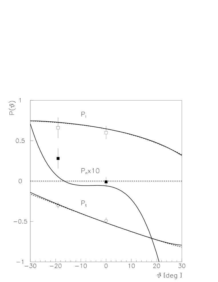
Figure 4.11: $\vartheta$-dependence of the recoil proton polarization components $P_{\ell}$ (open squares), $P_{n}$ (solid squares) and $P_{t}$ (open circles) in the quasi–elastic region of the $d({\vec{e}},e^{\prime}{\vec{p}})n$ reaction from Ref. [85]. The corresponding predictions, for the Paris DWF are shown (solid lines). The dashed lines correspond to the calculations without FSI effects.The results for the normal component have been magnified by a factor ten.

The data in Ref. [85] have been compared with a nonrelativistic calculation which includes FSI, meson-exchange currents, and isobar configurations, as well as leading order relativistic corrections from H. Arenhovel. The prediction from the present model is very close to the one reported in the paper [85].

The calculated $P_{t}$-component ($P_{x}$ according to the notation of the paper [83]), for the kinematical conditions of the experiment [83], is shown in Fig. 4.12. In this experiment the recoil-neutron momentum $p_{m}$ $\leq$ 100 MeV/c. Therefore, the polarization component is insensitive to the choice of the DWF model. The influence of the FSI effects on this observables is also small.

Figure 4.12: $\vartheta$-dependence of the proton polarization $P_{t}$ calculated for various DWFs. Predictions for the Paris wave function (solid line), the charge-dependent Bonn wave function (dashed line) are almost overlapping. Data and kinematical conditions are from Ref. [83]

We calculated the discussed polarization observables for the kinematical conditions of the experiment [84]. The recoil momentum of the neutron was restricted in this experiment to the range $0-60$ MeV/c. So, we averaged the predicted values over this momentum range. Due to the low value of the missing momentum the predicted observables are insensitive to the choice of DWF model and to the inclusion of FSI contribution. The predicted polarization components are presented in the Table 4.4. We see that the data are consistent with our theoretical calculations.

A discussion concerning the experimental evidence of the validity of IA in the quasi-elastic region is given in Ref. [86]. Disentangling medium modification of nucleon properties from additional reaction mechanisms remains a central problem in intermediate energy nuclear physics [86], for which polarization measurements can bring unique information.

$Q^{2}$ [GeV2]	$P_{l}$	$P_{t}$	$P_{n}$
0.38	0.60$\pm$ 0.07	-0.48$\pm$ 0.02	0.001$\pm$ 0.005	Experiment
0.38	0.63	-0.51	-0.008	Theory
0.50	0.77$\pm$ 0.04	-0.41$\pm$ 0.02	0.005$\pm$ 0.005	Experiment
0.50	0.85	-0.43	-0.002	Theory

Table 4.4: The recoil proton polarization observables from the experiment [84] and from the present calculation averaged over the neutron missing-momentum range $p_{m}$=0-60 MeV/c. The calculation corresponds to the Paris DWF.

4.4 Neutron polarization in case of unpolarized deuteron target

The polarization of the neutron, emitted in the reaction $\vec{e}+d\to e+\vec{n}+p$, is determined by the ${\vec{N}}_{ij}$ tensor:

$${\vec{N}}_{ij}=-TrF_{i}{\vec{\sigma}}F_{j}^{+},\ \ i,j=x,y,z.$$ (4.13)

As in the case of the proton polarization, the tensor ${\vec{N}}_{ij}$ can be represented in the following general form:

$${\vec{N}}_{ij}=\hat{\vec{k}}N_{ij}^{(k)}+{\vec{m}}N_{ij}^{(m)}+{\vec{n}}N_{ij}^{(n)}$$

and we can express the tensor structure of the contributions $N_{ij}^{(k)},$ $N_{ij}^{(m)},$ and $N_{ij}^{(n)}$ in terms of SFs $N_{i}$, (which are determined by Eq. (4.11) after substituting $P_{i}\rightarrow N_{i}$). The neutron polarization is also driven by thirteen real SFs $N_{i}$ depending on three kinematical variables: $k^{2}$, $W$, and $t.$ The formulae for SFs $N_{i}$ in terms of the scalar amplitudes are given in Appendix 6.

The measurement of the $G_{En}~{}$form factor by means of the recoil–neutron polarization method in quasi-elastic $d(\vec{e},e^{\prime}\vec{n})p$ has been recently performed at JLab [27] for $Q^{2}$ up to $\simeq$ 1.5 GeV². The kinematics of the experiment is given in Table 4.5 and the calculations are presented in Figs. 4.13 and 4.14.

$Q^{2}$ [GeV2]	$E$ [GeV]	$E^{\prime}$ [GeV]	$\theta_{e}$ [deg]	$\varepsilon$
0.45	0.884	0.646	52.7	0.644
1.15	2.33	1.750	30.8	0.836
1.47	3.40	2.584	23.6	0.887

Table 4.5: Kinematical parameters for the JLab experiment [27].

Figure 4.13: $\vartheta$-dependence of the neutron transversal polarization in $d(\vec{e},e^{\prime}\vec{n})p$ at the kinematics in Tab. 4.5. The angle $\vartheta=180^{\circ}$ corresponds to quasi-elastic kinematics, i.e. the neutron and the virtual photon move in the same direction. Notations as in Fig. 4.5.

Figure 4.14: $\vartheta$-dependence of the neutron transversal polarization, in $d(\vec{e},e^{\prime}\vec{n})p$, for quasi-elastic kinematics, corresponding to Ref. [27]. Notations as in Fig. 4.5.

4.5 Neutron polarization in case of vector-polarized deuteron target

The polarization state of the neutron, produced in the ${\vec{d}}(e,e^{\prime}{\vec{n}})p$ reaction (deuteron in this case is vector-polarized), is determined by the ${\vec{N}}_{ij}(\vec{\xi})$ tensor:

$${\vec{N}}_{ij}({\vec{\xi}})=-TrF_{i}{\vec{\sigma}}F_{j}^{+},\ \ i,j=x,y,z.$$ (4.14)

The tensor ${\vec{N}}_{ij}(\vec{\xi})$ can be represented in the following general form, as it was previously done for the case of the neutron polarization:

$${\vec{N}}_{ij}(\vec{\xi})={\vec{\xi}}{\vec{m}}{\vec{N}}_{ij}^{(m)}+{\vec{\xi}}{\vec{n}}{\vec{N}}_{ij}^{(n)}+{\vec{\xi}}{\vec{\hat{k}}}{\vec{N}}_{ij}^{(k)}.$$

The tensors ${\vec{N}}_{ij}^{(l)},$ $l=m,n,k$ can be expanded over a complete set of orthonormal vectors. For these tensors we have following general structure:

$${\vec{N}}_{ij}^{(m)} = N_{ij}^{(mk)}{\vec{\hat{k}}}+N_{ij}^{(mm)}{\vec{m}}+N_{ij}^{(mn)}{\vec{n}},$$

$${\vec{N}}_{ij}^{(k)} = N_{ij}^{(kk)}{\vec{\hat{k}}}+N_{ij}^{(km)}{\vec{m}}+N_{ij}^{(kn)}{\vec{n}},$$

$${\vec{N}}_{ij}^{(n)} = N_{ij}^{(nk)}{\vec{\hat{k}}}+N_{ij}^{(nm)}{\vec{m}}+N_{ij}^{(nn)}{\vec{n}}.$$

The tensors $N_{ij}^{(lr)},$ $l,r=m,n,k$ can be decomposed, in turn, in the way that was used in the analysis of previous observables. In terms of SFs, we may write these tensors as follows

$$N_{ij}^{(mk)}= D_{1}\hat{k}_{i}\hat{k}_{j}+D_{2}m_{i}m_{j}+D_{3}n_{i}n_{j}+D_{4}\{\hat{k},m\}_{ij}+iD_{5}[\hat{k},m]_{ij},$$

$$N_{ij}^{(mm)}= D_{6}\hat{k}_{i}\hat{k}_{j}+D_{7}m_{i}m_{j}+D_{8}n_{i}n_{j}+D_{9}\{\hat{k},m\}_{ij}+iD_{10}[\hat{k},m]_{ij},$$

$$N_{ij}^{(mn)}= D_{11}\{\hat{k},n\}_{ij}+D_{12}\{m,n\}_{ij}+iD_{13}[\hat{k},n]_{ij}+iD_{14}[m,n]_{ij},$$

$$N_{ij}^{(kk)}= D_{15}\hat{k}_{i}\hat{k}_{j}+D_{16}m_{i}m_{j}+D_{17}n_{i}n_{j}+D_{18}\{\hat{k},m\}_{ij}+iD_{19}[\hat{k},m]_{ij},$$

$$N_{ij}^{(km)}= D_{20}\hat{k}_{i}\hat{k}_{j}+D_{21}m_{i}m_{j}+D_{22}n_{i}n_{j}+D_{23}\{\hat{k},m\}_{ij}+iD_{24}[\hat{k},m]_{ij},$$

$$N_{ij}^{(kn)}= D_{25}\{\hat{k},n\}_{ij}+D_{26}\{m,n\}_{ij}+iD_{27}[\hat{k},n]_{ij}+iD_{28}[m,n]_{ij},$$

$$N_{ij}^{(nk)}= D_{29}\{\hat{k},n\}_{ij}+D_{30}\{m,n\}_{ij}+iD_{31}[\hat{k},n]_{ij}+iD_{32}[m,n]_{ij},$$

$$N_{ij}^{(nm)}= D_{33}\{\hat{k},n\}_{ij}+D_{34}\{m,n\}_{ij}+iD_{35}[\hat{k},n]_{ij}+iD_{36}[m,n]_{ij},$$

$$N_{ij}^{(nn)}= D_{37}\hat{k}_{i}\hat{k}_{j}+D_{38}m_{i}m_{j}+D_{39}n_{i}n_{j}+D_{40}\{\hat{k},m\}_{ij}+iD_{41}[\hat{k},m]_{ij}.$$

Thus, the dependence of the neutron polarization on the vector polarization of the deuteron is determined by forty-one SFs $D_{i}$, $i=1-41$. The formulae for SFs $D_{i}$ in terms of the reaction scalar amplitudes are given in Appendix 7.

The components of the neutron polarization vector, $\vec{P}(n)$, can be written as

$$P_{i}(n)=P_{ij}\xi_{j}.$$ (4.16)

The polarization components have a definite general structure, if we single out the explicit dependences on the azimuthal angle $\phi,$ virtual-photon linear polarization $\varepsilon,$ and contributions of the longitudinal $(L)$ and transverse $(T)$ components of the electromagnetic current of the $\gamma^{*}d\rightarrow np$ reaction. As a result, we can obtain:

For the $P_{x}$-component:

$$P_{xx}\sigma_{0} = {\cal N}[P_{xx}^{(TT)}+\varepsilon P_{xx}^{(LL)}+\sqrt{2\varepsilon(1+\varepsilon)}cos\phi P_{xx}^{(LT)}+\varepsilon cos(2\phi)\bar{P}_{xx}^{(TT)}],$$

$$P_{xy}\sigma_{0} = {\cal N}sin\phi[\sqrt{2\varepsilon(1+\varepsilon)}P_{xy}^{(LT)}+\varepsilon cos\phi P_{xy}^{(TT)}],$$

$$P_{xz}\sigma_{0} = {\cal N}[P_{xz}^{(TT)}+\varepsilon P_{xz}^{(LL)}+\sqrt{2\varepsilon(1+\varepsilon)}cos\phi P_{xz}^{(LT)}+\varepsilon cos(2\phi)\bar{P}_{xz}^{(TT)}],$$

where

$$P_{xx}^{(TT)} = D_{7}+D_{8},~{}P_{xx}^{(LL)}=2\displaystyle\frac{Q^{2}}{k^{2}_{0}}D_{6},~{}\bar{P}_{xx}^{(TT)}=D_{7}-D_{8},\ \ P_{xx}^{(LT)}=-2\displaystyle\frac{\sqrt{Q^{2}}}{k_{0}}D_{9},$$

$$P_{xy}^{(TT)} = 4D_{34},~{}P_{xy}^{(LT)}=-2\displaystyle\frac{\sqrt{Q^{2}}}{k_{0}}D_{33},~{}P_{xz}^{(TT)}=D_{21}+D_{22},~{}\bar{P}_{xz}^{(TT)}=D_{21}-D_{22},$$

$$P_{xz}^{(LL)} = 2\displaystyle\frac{Q^{2}}{k^{2}_{0}}D_{20},~{}P_{xz}^{(LT)}=-2\displaystyle\frac{\sqrt{Q^{2}}}{k_{0}}D_{23},$$

For the $P_{y}$-component:

$$P_{yx}\sigma_{0} = {\cal N}sin\phi[\sqrt{2\varepsilon(1+\varepsilon)}P_{yx}^{(LT)}+\varepsilon cos\phi P_{yx}^{(TT)}],$$

$$P_{yy}\sigma_{0} = {\cal N}[P_{yy}^{(TT)}+\varepsilon P_{yy}^{(LL)}+\sqrt{2\varepsilon(1+\varepsilon)}cos\phi P_{yy}^{(LT)}+\varepsilon cos(2\phi)\bar{P}_{yy}^{(TT)}],$$

$$P_{yz}\sigma_{0} = {\cal N}sin\phi[\sqrt{2\varepsilon(1+\varepsilon)}P_{yz}^{(LT)}+\varepsilon cos\phi P_{yz}^{(TT)}],$$

where

$$P_{yx}^{(TT)} = 4D_{12},~{}P_{yx}^{(LT)}=-2\displaystyle\frac{\sqrt{Q^{2}}}{k_{0}}D_{11},~{}P_{yy}^{(TT)}=D_{38}+D_{39},~{}\bar{P}_{yy}^{(TT)}=D_{38}-D_{39},$$

$$P_{yy}^{(LL)} = 2\displaystyle\frac{Q^{2}}{k^{2}_{0}}D_{37},~{}P_{yy}^{(LT)}=-2\displaystyle\frac{\sqrt{Q^{2}}}{k_{0}}D_{40},$$

$$P_{yz}^{(TT)} = 4D_{26},~{}P_{yz}^{(LT)}=-2\displaystyle\frac{\sqrt{Q^{2}}}{k_{0}}D_{25},$$

For the $P_{z}$-component:

$$P_{zx}\sigma_{0} = {\cal N}[P_{zx}^{(TT)}+\varepsilon P_{zx}^{(LL)}+\sqrt{2\varepsilon(1+\varepsilon)}cos\phi P_{zx}^{(LT)}+\varepsilon cos(2\phi)\bar{P}_{zx}^{(TT)}],$$

$$P_{zy}\sigma_{0} = {\cal N}sin\phi[\sqrt{2\varepsilon(1+\varepsilon)}P_{zy}^{(LT)}+\varepsilon cos\phi P_{zy}^{(TT)}],$$

$$P_{zz}\sigma_{0} = {\cal N}[P_{zz}^{(TT)}+\varepsilon P_{zz}^{(LL)}+\sqrt{2\varepsilon(1+\varepsilon)}cos\phi P_{zz}^{(LT)}+\varepsilon cos(2\phi)\bar{P}_{zz}^{(TT)}],$$

where

$$P_{zx}^{(TT)} = D_{2}+D_{3},~{}P_{zx}^{(LL)}=2\displaystyle\frac{Q^{2}}{k^{2}_{0}}D_{1},~{}\bar{P}_{zx}^{(TT)}=D_{2}-D_{3},~{}P_{zx}^{(LT)}=-2\displaystyle\frac{\sqrt{Q^{2}}}{k_{0}}D_{4},$$

$$P_{zy}^{(TT)} = 4D_{30},~{}P_{zy}^{(LT)}=-2\displaystyle\frac{\sqrt{Q^{2}}}{k_{0}}D_{29},~{}P_{zz}^{(TT)}=D_{16}+D_{17},~{}\bar{P}_{zz}^{(TT)}=D_{16}-D_{17},$$

$$P_{zz}^{(LL)} = 2\displaystyle\frac{Q^{2}}{k^{2}_{0}}D_{15},~{}P_{zz}^{(LT)}=-2\displaystyle\frac{\sqrt{Q^{2}}}{k_{0}}D_{18}.$$

As it was shown earlier, the components of the neutron polarization, containing the terms with the longitudinal contribution of the electromagnetic current, are the most sensitive to the form factor $G_{En}$. For coplanar experimental conditions ($\phi=0^{0}$ or $180^{0}$) the following components are nonzero: $P_{xx}$, $P_{xz}$, $P_{yy}$, $P_{zx}$, and $P_{zz}$.

4.6 Proton polarization in case of vector–polarized deuteron target

A new method for determination of the neutron electric form factor has been suggested in Ref. [87]. This method requires no longitudinally polarized electron beam and is based on measurement of the polarization of the nucleons (protons or neutrons) produced in the disintegration of the vector polarized deuteron. The sensitivity of the spin transfer coefficients to the form factor $G_{En},$ as well as to various parameterizations of the deuteron wave functions has been analyzed for the case of the reaction ${\vec{d}}(e,e^{\prime}{\vec{p}})n.$ The analysis was carried out in the framework of RIA. It was shown that in the region of the quasi–elastic peak some spin transfer coefficients are large and sensitive to the form factor $G_{En}$ and practically do not depend on the choice of the deuteron wave function. Later, the outgoing nucleon polarization in the case of polarized beam and target (the vector and tensor deuteron polarizations were considered) has been investigated in Ref. [88]. In the numerical applications, they have studied all the nonvanishing components of proton and neutron polarization in the coplanar kinematics and in the quasi–elastic region. The calculations were made in the standard theory with emphasis on the effect of nucleonic and pionic relativistic corrections. It was shown, in particular, that the longitudinal component of neutron polarization with vector polarized deuterons is as sensitive to the parametrization of the form factor $G_{En}$ as the sideways beam polarization transfer.

In this chapter we present the formulae describing the polarization state of the proton, produced in the ${\vec{d}}(e,e^{\prime}{\vec{p}})n$ reaction (where the deuteron is vector–polarized). The polarization of the proton is determined by the ${\vec{P}}_{ij}({\vec{\xi}})$ tensor:

$${\vec{P}}_{ij}({\vec{\xi}})=Tr{\vec{\sigma}}F_{i}F_{j}^{+}.$$ (4.17)

The tensor ${\vec{P}}_{ij}({\vec{\xi}})$ can be represented in the following general form

$${\vec{P}}_{ij}({\vec{\xi}})={\vec{\xi}}\cdot{\vec{m}}{\vec{P}}_{ij}^{(m)}+{\vec{\xi}}\cdot{\vec{n}}{\vec{P}}_{ij}^{(n)}+{\vec{\xi}}\cdot\hat{\vec{k}}{\vec{P}}_{ij}^{(k)}.$$ (4.18)

The tensors ${\vec{P}}_{ij}^{(l)},l=m,n,k$ can be expanded over the complete set of the orthonormal vectors. As a result, we have following general structures for these tensors

$${\vec{P}}_{ij}^{(m)}=\bar{P}_{ij}^{(mk)}{\hat{\vec{k}}}+\bar{P}_{ij}^{(mm)}{\vec{m}}+\bar{P}_{ij}^{(mn)}{\vec{n}},$$

$${\vec{P}}_{ij}^{(k)}=\bar{P}_{ij}^{(kk)}{\hat{\vec{k}}}+\bar{P}_{ij}^{(km)}{\vec{m}}+\bar{P}_{ij}^{(kn)}{\vec{n}},$$ (4.19)

$${\vec{P}}_{ij}^{(n)}=\bar{P}_{ij}^{(nk)}{\hat{\vec{k}}}+\bar{P}_{ij}^{(nm)}{\vec{m}}+\bar{P}_{ij}^{(nn)}{\vec{n}}.$$

The tensors $\bar{P}_{ij}^{(lr)},l,r=m,n,k$ can be decomposed, in turn, in the way that was used in previous chapter. Then these tensors have the same form as the tensors $N_{ij}^{(lr)}$ (see formula (4.14)), describing the neutron polarization, where SFs $D_{i}$ are replaced by SFs $B_{i}$. Thus, the dependence of the proton polarization on the vector polarization of the deuteron is determined by forty-one SFs $B_{i},i=1-41.$ The formulae for SFs $B_{i}$ in terms of the reaction scalar amplitudes are given in Appendix 8.

The components of the proton polarization vector, $\vec{P}(p)$, can be written as

$$P_{i}(p)=\bar{P}_{ij}\xi_{j}.$$ (4.20)

The polarization components have definite general structure, if we single out the explicit dependences on the azimuthal angle $\phi,$ virtual–photon linear polarization $\varepsilon,$ and contributions of the longitudinal (L) and transverse (T) components of the electromagnetic current of the $\gamma^{*}d\rightarrow np$ reaction. The expressions for the $\bar{P}_{ij}$ quantities can be obtained from the formulae for the $P_{ij}$ quantities by following substitution $D_{i}\rightarrow B_{i}.$ Let us note that the components of the proton polarization, containing the terms with the longitudinal contribution of the electromagnetic current, will be the most sensitive to the form factor $G_{En}.$ For coplanar experimental conditions ($\phi=0^{0}$ or $\phi=180^{0}$) the following components are nonzero: $\bar{P}_{xx},$ $\bar{P}_{xz},$ $\bar{P}_{yy},$ $\bar{P}_{zx},$ and $\bar{P}_{zz}.$

4.7 Disintegration of tensor–polarized deuteron target by unpolarized electron beam

The differential cross section of the tensor–polarized deuteron disintegration by the unpolarized electron beam (in the coincidence experimental setup) has the following general structure (where the $z$ axis is directed along the virtual–photon momentum ${\vec{k}}$, and the $xz$ plane coincides with the $({\vec{k}},{\vec{p}})$ plane):

$$\frac{d^{3}\sigma}{dE^{\prime}d\Omega_{e}d\Omega_{p}} = N\left\{\sigma_{T}+A_{xz}^{T}Q_{xz}+A_{xx}^{T}(Q_{xx}-Q_{yy})+A_{zz}^{T}Q_{zz}+\right.$$

$$\varepsilon\left[\sigma_{L}+A_{xz}^{L}Q_{xz}+A_{xx}^{L}(Q_{xx}-Q_{yy})+A_{zz}^{L}Q_{zz}\right]+$$

$$\sqrt{2\varepsilon(1+\varepsilon)}\cos\phi\left[\sigma_{I}+A_{xz}^{I}Q_{xz}+A_{xx}^{I}(Q_{xx}-Q_{yy})+A_{zz}^{I}Q_{zz}\right]+$$

$$\sqrt{2\varepsilon(1+\varepsilon)}\sin\phi(A_{xy}^{I}Q_{xy}+A_{yz}^{I}Q_{yz})+$$

$$\varepsilon\sin 2\phi(A_{xy}^{P}Q_{xy}+A_{yz}^{P}Q_{yz})+$$

$$\left.\varepsilon\cos 2\phi\left[\sigma_{P}+A_{xz}^{P}Q_{xz}+A_{xx}^{P}(Q_{xx}-Q_{yy})+A_{zz}^{P}Q_{zz}\right]\right\},$$

where the quantities $Q_{ij},\ (i,j=x,y,z)$ are the components of the quadrupole–polarization tensor of the deuteron in its rest system (the coordinate system is specified similarly to the case of the np–pair CMS). These components satisfy to the following conditions: $Q_{ij}=Q_{ji},\$ $Q_{ii}=0.$

The general characteristic property of all these tensor asymmetries is that they vanish in the region of the quasi–elastic scattering. This can be explained as follows. All the asymmetries are determined by the convolution $X_{\mu\nu}Q_{\mu\nu},$ where the tensor $X_{\mu\nu}$ is built with the four-momenta describing the $d\rightarrow np$ transition. Due to the condition $P_{\mu}Q_{\mu\nu}=0,$ the most general form of this tensor is

$$X_{\mu\nu}=a_{1}g_{\mu\nu}+ia_{2}[\gamma_{\mu},\gamma_{\nu}]+a_{3}\gamma_{\mu}p_{\nu}+a_{4}\gamma_{\nu}p_{\mu}+a_{5}p_{\mu}p_{\nu},$$

where $p_{\mu}$ is the four-momentum of the neutron–spectator. However, if we take into account that $Q_{\mu\nu}g_{\mu\nu}=0,\ Q_{\mu\nu}=Q_{\nu\mu},$ then the convolution $X_{\mu\nu}Q_{\mu\nu}$ is determined by $a_{3}$, $a_{4}$, and $a_{5}$. From the condition $P_{\mu}Q_{\mu\nu}=0$, it follows that the time components of the $Q_{\mu\nu}$ tensor are zero in the laboratory system. After all, the convolution $X_{\mu\nu}Q_{\mu\nu}$ turns out proportional to the nucleon–spectator three-momentum which is zero in the peak of the quasi–elastic scattering.

Thus, in the general case the exclusive cross section of the electrodisintegration of the tensor–polarized deuteron is determined by 16 independent asymmetries $A_{ij}^{m}(W,k^{2},\vartheta),$ where $i,j=x,y,z;m=T,P,L,I.$ The asymmetries $A_{ij}^{m}$ can be related to 18 independent scalar amplitudes $f_{i},(i=1-18)$ describing the $\gamma^{*}+d\rightarrow n+p$ reaction. These relations are:

$$A_{xz}^{T} = 4\frac{\omega}{M}Re(f_{1}f_{3}^{*}+f_{2}f_{4}^{*}+f_{7}f_{9}^{*}+f_{8}f_{10}^{*}),$$

$$A_{xx}^{T} = |f_{3}|^{2}+|f_{4}|^{2}+|f_{9}|^{2}+|f_{10}|^{2}-|f_{5}|^{2}-|f_{6}|^{2}-|f_{11}|^{2}-|f_{12}|^{2},$$

$$A_{zz}^{T} = 2\frac{\omega^{2}}{M^{2}}\left[|f_{1}|^{2}+|f_{2}|^{2}+|f_{7}|^{2}+|f_{8}|^{2}-\frac{M^{2}}{\omega^{2}}(|f_{5}|^{2}+|f_{6}|^{2}+|f_{11}|^{2}+|f_{12}|^{2})\right]-A_{xx}^{T},$$

$$A_{xz}^{I} = -4\frac{\omega}{M}\frac{\sqrt{-k^{2}}}{k_{0}}Re(f_{1}f_{15}^{*}+f_{3}f_{13}^{*}+f_{2}f_{16}^{*}+f_{4}f_{14}^{*}),$$

$$A_{xx}^{I} = -2\frac{\sqrt{-k^{2}}}{k_{0}}Re(f_{3}f_{15}^{*}+f_{4}f_{16}^{*}-f_{5}f_{17}^{*}-f_{6}f_{18}^{*}),$$

$$A_{zz}^{I} = -4\frac{\omega^{2}}{M^{2}}\frac{\sqrt{-k^{2}}}{k_{0}}Re\left[f_{1}f_{13}^{*}+f_{2}f_{14}^{*}-\frac{M^{2}}{\omega^{2}}(f_{5}f_{17}^{*}+f_{6}f_{18}^{*})\right]-A_{xx}^{I},$$

$$A_{xy}^{I} = -4\frac{\sqrt{-k^{2}}}{k_{0}}Re(f_{9}f_{17}^{*}+f_{10}f_{18}^{*}+f_{12}f_{18}^{*}+f_{11}f_{15}^{*}),$$

$$A_{yz}^{I} = -4\frac{\omega}{M}\frac{\sqrt{-k^{2}}}{k_{0}}Re(f_{7}f_{17}^{*}+f_{8}f_{18}^{*}+f_{12}f_{14}^{*}+f_{11}f_{13}^{*}),$$

$$A_{xz}^{L} = -8\frac{\omega}{M}\frac{k^{2}}{k_{0}^{2}}Re(f_{13}f_{15}^{*}+f_{14}f_{16}^{*}),$$

$$A_{xx}^{L} = -2\frac{k^{2}}{k_{0}^{2}}[|f_{15}|^{2}+|f_{16}|^{2}-|f_{17}|^{2}-|f_{18}|^{2}],$$

$$A_{zz}^{L} = -4\frac{\omega^{2}}{M^{2}}\frac{k^{2}}{k_{0}^{2}}\left[|f_{13}|^{2}+|f_{14}|^{2}-\frac{M^{2}}{\omega^{2}}(|f_{17}|^{2}+|f_{18}|^{2})\right]-A_{xx}^{L},$$

$$A_{xy}^{P} = 4Re(f_{5}f_{9}^{*}+f_{6}f_{10}^{*}+f_{4}f_{12}^{*}+f_{3}f_{11}^{*}),$$

$$A_{yz}^{P} = 4\frac{\omega}{M}Re(f_{5}f_{7}^{*}+f_{6}f_{8}^{*}+f_{2}f_{12}^{*}+f_{1}f_{11}^{*}),$$

$$A_{xz}^{P} = 4\frac{\omega}{M}Re(f_{1}f_{3}^{*}+f_{2}f_{4}^{*}-f_{7}f_{9}^{*}-f_{8}f_{10}^{*}),$$

$$A_{xx}^{P} = |f_{3}|^{2}+|f_{4}|^{2}-|f_{9}|^{2}-|f_{10}|^{2}-|f_{5}|^{2}-|f_{6}|^{2}+|f_{11}|^{2}+|f_{12}|^{2},$$

$$A_{zz}^{P} = 2\frac{\omega^{2}}{M^{2}}\left[|f_{1}|^{2}+|f_{2}|^{2}-|f_{7}|^{2}-|f_{8}|^{2}-\frac{M^{2}}{\omega^{2}}(|f_{5}|^{2}+|f_{6}|^{2}-|f_{11}|^{2}-|f_{12}|^{2})\right]-A_{xx}^{P}.$$

One can see from this formula that the scattering of unpolarized electrons by a tensor polarized deuteron target with components $Q_{xy}=Q_{yz}=0$, is characterized by the same $\phi-$ and $\varepsilon-$ dependences as in the case of the scattering of unpolarized electrons by the unpolarized target. If $Q_{xy}\neq 0,$ $Q_{yz}\neq 0$, then new tems of the type $\sqrt{2\varepsilon(1+\varepsilon)}\sin\phi$ and $\varepsilon\sin 2\phi$ are present in the cross section. The asymmetries with upper indices $T,P(L)$ are determined only by the transverse (longitudinal) components of the electromagnetic current for the $\gamma^{*}+d\rightarrow n+p$ reaction, while the asymmetries with upper index $I$ are determined by the interference of the longitudinal and transverse components of the electromagnetic current.

Chapter 5 Conclusions

We developed a relativistic approach to the calculation of the differential cross section and various polarization observables for the deuteron electrodisintegration process, $e^{-}+d\rightarrow e^{-}+n+p.$ Our formalism is based on the most general symmetry properties of the hadron electromagnetic interaction, such as gauge invariance (the conservation of the hadronic and leptonic electromagnetic currents) and P–invariance (invariance with respect to the space reflections) and does not depend on the deuteron structure and on the details of the reaction mechanism for $\gamma^{*}+d\rightarrow n+p.$

We established a general formalism for the structure of the differential cross section and various polarization observables. This general analysis was done with the help of the structure function formalism which is especially convenient for the investigation of the polarization phenomena in this reaction.

The observables related to the cases of a polarized deuteron target, longitudinally polarized electron beam, polarizations of the outgoing nucleons (proton and neutron), as well as the polarization transfer from electron to final nucleon and from deuteron (vector–polarized) to nucleon, and the correlation of the electron and deuteron polarizations were considered in detail.

For the quantitative estimations of the observables a dynamical model of the $\gamma^{*}+d\rightarrow n+p$ reaction was developed: the relativistic impulse approximation which accounts for four Feynman diagrams: two diagrams represent the relativized description of the one–nucleon–exchange mechanism, and the others are the deuteron–exchange and contact diagrams. The deuteron structure is described here by the relativistic form factors of the $dnp-$vertex with one virtual nucleon. In order to calculate the dependence of these form factors on the nucleon virtuality we use the approach developed by the Buck and Gross [39]. The resulting amplitude for the $\gamma^{*}+d\rightarrow n+p$ reaction can be unambiguously calculated for any values of the kinematics variables $Q^{2},s$ and $t$.

The RIA amplitude does not contain the effects of the $np\rightarrow np$ scattering. These effects are also included in nonrelativistic models of the deuteron electrodisintegration in terms of the FSI effects. In relativistic physics, this process (the $np\rightarrow np$ scattering) is required by the fulfilment of the unitarity condition. This is especially important for the analysis of the polarization effects in $e^{-}+d\rightarrow e^{-}+n+p$ reaction - for example, the asymmetry of unpolarized electrons inclusively scattered by a vector–polarized target, ${\vec{d}}(e,e^{\prime})np.$

The proposed unitarization procedure is carried out in the relativistic approach, for any value of $Q^{2}$. We also use a relativistic description of the nucleon electromagnetic current in terms of the Dirac ($F_{1}$) and Pauli ($F_{2}$) form factors. The $np$ phase shifts were taken from Ref. [64].

We calculated the asymmetry $\Sigma_{e}$ for the deuteron disintegration by longitudinally polarized electron beam. It is a T–odd polarization observable determined by the so–called fifth SF, $\alpha_{5}.$ In impulse approximation this asymmetry is zero.

The predicted value for the asymmetry $\Sigma_{e}$ for the kinematics conditions of the experiment performed at the MIT–Bates [21] (measurements were done at the missing momentum of 210 MeV/c) does not contradict the experimental data. The sensitivity of this asymmetry to the choice of DWFs appears only in the region where $p_{m}\geq~{}280~{}MeV/c.$ The qualitative behaviour of this asymmetry as a function of $p_{m}$, predicted in our model, is consistent with one in Ref. [69]. The predicted asymmetry for the experimental conditions of Ref. [76] agree relatively well with the data.

The sideways asymmetry $A_{x}^{ed}$ (the vector–polarized deuteron disintegration by the longitudinally polarized electron beam) has been measured at the NIKHEF accelerator [20] for missing momenta less than 200 MeV/c. The agreement of the predicted $A_{x}^{ed}$ with the experimental data is excellent, particularly in the quasi–elastic region. The sensitivity of the asymmetry to the choice of the DWF model is small and influence of the FSI effects is also insignificant. Therefore, the measurement of this asymmetry in the quasi–elastic region can give a reliable value of the $G_{En}$ form factor.

We suggested a method for the determination of the $G_{En}$ form factor, at relatively large $Q^{2}$, from the ratio $R=A_{x}/A_{z}$ of the T–even asymmetries in ${\vec{d}}({\vec{e}},e^{\prime}p)n$ reaction, measured in the kinematical conditions of the quasi–elastic $en$–scattering. This method seems promising and may be comparable in accuracy with the measurements of the $G_{Ep}$ form factor through the recoil polarization method.

We calculated the proton polarization in $d(e,e{\vec{p}})n$ and $d({\vec{e}},e{\vec{p}})n$ reactions and compared the results with existing experimental data. The calculations of the polarization transfer components $P_{l}$ and $P_{t}$ describe the data, obtained at MIT in the region of the neutron recoil momenta lower than $100~{}MeV/c,$ well, but calculations of the induced polarization $P_{n}$ at $p_{m}=100~{}MeV/c$ somewhat underestimate the experimental result. The data from Ref. [84] are also consistent with our theoretical calculations of these quantities.

In conclusion we can say that we developed a fully relativistic model for the description of various polarization effects in the deuteron electrodisintegration reaction. The reliability of the suggested model was tested by comparing the predicted results of our model with the existing experimental data. The agreement is quite reasonable. This model is especially adapted to the description of the deuteron electrodisintegration reaction at large $Q^{2}$ where relativistic effects must be sizeable.

Chapter 6 Appendices

6.1 Appendix 1: relations between invariant amplitudes and scalar amplitudes

The scalar amplitudes $F_{i}$ are related to the invariant amplitudes $H_{i}$ in the following way:

$$F_{1} = -H_{18}-\frac{W}{\omega}\frac{{\vec{p}}\cdot{\vec{k}}}{m^{2}}H_{13}-2\frac{{\vec{p}}^{2}}{m^{2}}H_{14},$$

$$F_{2} = \frac{1}{m^{2}}\biggl{[}{\vec{k}}^{2}\frac{W}{\omega}H_{13}+2{\vec{p}}\cdot{\vec{k}}(H_{14}+H_{15})-Wk_{0}H_{16}-2k^{2}H_{17}\biggr{]},$$

$$F_{3} = \frac{1}{m^{2}}\biggl{(}2H_{17}+\frac{W}{\omega}H_{13}\biggr{)},\ \ F_{4}=\frac{2}{m^{2}}\biggl{(}H_{14}+H_{15}\biggr{)},$$

$$F_{5} = \frac{1}{2m\omega}\biggl{[}2Wk_{0}H_{13}+4(k^{2}H_{17}+Ek_{0}H_{16}-{\vec{p}}\cdot{\vec{k}}H_{15})+$$

$$+W^{2}(H_{8}-\frac{k^{2}}{m^{2}}H_{9}+\frac{Ek_{0}}{m^{2}}H_{11}-\frac{{\vec{p}}\cdot{\vec{k}}}{m^{2}}H_{12}-2\frac{{\vec{p}}\cdot{\vec{k}}}{W^{2}}H_{18})\biggr{]},$$

$$F_{6} = \frac{k_{0}}{m}\biggl{(}2H_{14}-H_{18}\biggr{)}-\frac{W}{m^{3}}\biggl{(}k^{2}H_{10}+{\vec{p}}\cdot{\vec{k}}H_{11}-Ek_{0}H_{12}\biggr{)},$$

$$F_{7} = 2\frac{k_{0}}{m}H_{17}-\frac{W}{4m^{3}}\biggl{(}{\vec{p}}\cdot{\vec{k}}H_{6}+Ek_{0}H_{7}\biggr{)},\ \$$

$$F_{8} = \frac{k_{0}}{m}(2H_{15}+H_{18})+\frac{W}{4m^{3}}(2Wk_{0}-k^{2})H_{6},$$

$$F_{9} = -\frac{W}{2m}H_{8},\ \ F_{10}=\frac{1}{m^{2}}\biggl{(}{\vec{p}}\cdot{\vec{k}}H_{1}+Ek_{0}H_{2}+k^{2}H_{3}+{\vec{p}}\cdot{\vec{k}}\frac{m}{E+m}H_{8}\biggr{)},$$

$$F_{11} = \frac{1}{2m\omega}(4H_{17}-\frac{W^{2}}{m^{2}}H_{9}),\ \ F_{12}=-\frac{W}{m^{3}}H_{10},$$

$$F_{13} = \frac{1}{2m\omega}(\frac{W^{2}}{m^{2}}H_{12}+4H_{15}+2H_{18}),\ \ F_{14}=\frac{W}{m^{3}}H_{11},$$

$$F_{15} = \frac{1}{m^{2}}\frac{W}{\omega}\biggl{[}H_{3}+\frac{1}{W}\frac{{\vec{p}}\cdot{\vec{k}}}{E+m}(\frac{W}{m}H_{9}+2H_{17})\biggr{]},$$

$$F_{16} = \frac{1}{2m^{4}}\biggl{[}-{\vec{p}}\cdot{\vec{k}}H_{4}-Ek_{0}H_{5}+{\vec{p}}\cdot{\vec{k}}\frac{m}{E+m}(H_{6}+4H_{10})+\frac{mk_{0}}{E+m}(EH_{7}+4mH_{17})\biggr{]},$$

$$F_{17} = -\frac{1}{m^{2}}\frac{W}{\omega}\biggl{[}H_{11}+\frac{m}{E+m}(H_{8}-\frac{k^{2}}{m^{2}}H_{9}+\frac{Ek_{0}}{m^{2}}H_{11})-$$

$$-\frac{k_{0}}{E+m}(H_{13}+H_{16}+2\frac{k^{2}}{Wk_{0}}H_{17})\biggr{]},$$

$$F_{18} = \frac{2}{m^{2}}\frac{k_{0}}{E+m}\biggl{[}H_{14}+H_{15}+\frac{E}{m}(\frac{k^{2}}{Ek_{0}}H_{10}-H_{12})+$$

$$+\frac{2Wk_{0}-k^{2}}{4m^{2}}\frac{E+m}{k_{0}}(H_{4}-\frac{m}{E+m}H_{6})\biggr{]},$$

where $W$ is the total energy of the $np-$pair; $E,\omega,k_{0}$ are the energies of the nucleon, deuteron, virtual photon in the $np-$ pair CMS, repectively; ${\vec{p}}$ and ${\vec{k}}$ are the 3-momenta of the proton and virtual photon in the final–hadrons CMS.

6.2 Appendix 2: relations between two sets of scalar amplitudes

Here we give the explicit expression for the nonzero elements of the matrix $M_{ij},$ which relate two equivalent sets of the amplitudes $f_{i}$ and $F_{j}$ :

$$M_{2\ 5} = M_{3\ 9}=M_{5\ 1}=M_{8\ 5}=M_{11\ 9}=M_{13\ 5}=M_{13\ 7}=M_{13\ 9}=M_{16\ 7}=$$

$$= M_{18\ 7}=-M_{9\ 1}=|{\vec{k}}|,~{}M_{13\ 11}=|{\vec{k}}|^{3},$$

$$M_{2\ 6} = M_{3\ 10}=M_{5\ 2}=M_{8\ 6}=M_{11\ 10}=M_{13\ 6}=M_{13\ 8}=M_{13\ 10}=M_{16\ 8}=$$

$$= M_{18\ 8}=-M_{9\ 2}=|{\vec{p}}|\cos\vartheta,$$

$$M_{1\ 8} = M_{4\ 6}=M_{4\ 8}=M_{4\ 10}=M_{6\ 8}=M_{7\ 2}=M_{10\ 6}=M_{12\ 10}=M_{14\ 10}=$$

$$= M_{15\ 6}=-M_{17\ 2}=|{\vec{p}}|\sin\vartheta,$$

$$M_{13\ 12} = M_{13\ 13}=M_{13\ 15}={\vec{k}}\ ^{2}|{\vec{p}}|\cos\vartheta,M_{1\ 13}=M_{14\ 15}=M_{15\ 12}=M_{17\ 3}=$$

$$= {\vec{k}}\ ^{2}|{\vec{p}}|\sin\vartheta,$$

$$M_{13\ 14} = M_{13\ 16}=M_{13\ 17}={\vec{p}}\ ^{2}|{\vec{k}}|\cos^{2}\vartheta,$$

$$M_{2\ 17} = M_{3\ 14}=M_{5\ 4}=M_{16\ 16}={\vec{p}}\ ^{2}|{\vec{k}}|\sin^{2}\vartheta,$$

$$M_{1\ 14} = M_{1\ 17}=M_{14\ 16}=M_{14\ 17}=M_{15\ 14}=M_{15\ 16}=M_{17\ 4}={\vec{p}}\ ^{2}|{\vec{k}}|\cos\vartheta\sin\vartheta,$$

$$M_{13\ 18} = |{\vec{p}}|\ ^{3}\cos^{3}\theta,~{}M_{4\ 18}=|{\vec{p}}|\ ^{3}\sin^{3}\vartheta,~{}M_{1\ 18}=M_{14\ 18}=M_{15\ 18}=|{\vec{p}}|\ ^{3}\cos^{2}\vartheta\sin\vartheta,$$

$$M_{2\ 18} = M_{3\ 18}=M_{16\ 18}=|{\vec{p}}|\ ^{3}\cos\vartheta\sin^{2}\vartheta,$$

where $\vartheta$ is the angle between the 3-momenta of the proton and virtual photon in the final–hadrons CMS.

6.3 Appendix 3: expressions of SFs for $d(e,e^{\prime}p)n$ and $\vec{d}(\vec{e},e^{\prime}p)n$ in terms of the scalar amplitudes

Relations between SFs $\alpha_{i}$ $(i=1-5),$ $\beta_{i}$ $(i=1-13)$, $\gamma_{i}$ $(i=1-23),$ $\delta_{i}$ $(i=1-9)$ and the scalar amplitudes $f_{i}$ $(i=1-18)$ determining the $\gamma^{*}d\rightarrow np$ reaction

$$\alpha_{1} = \frac{2}{3}\biggl{[}\frac{\omega^{2}}{M^{2}}(|f_{13}|^{2}+|f_{14}|^{2})+|f_{15}|^{2}+|f_{16}|^{2}+|f_{17}|^{2}+|f_{18}|^{2}\biggr{]},$$

$$\alpha_{2} = \frac{2}{3}\biggl{[}\frac{\omega^{2}}{M^{2}}(|f_{7}|^{2}+|f_{8}|^{2})+|f_{9}|^{2}+|f_{10}|^{2}+|f_{11}|^{2}+|f_{12}|^{2}\biggr{]},$$

$$\alpha_{3} = \frac{2}{3}\biggl{[}\frac{\omega^{2}}{M^{2}}(|f_{1}|^{2}+|f_{2}|^{2})+|f_{3}|^{2}+|f_{4}|^{2}+|f_{5}|^{2}+|f_{6}|^{2}\biggr{]},$$

$$\alpha_{4} = \frac{2}{3}Re\biggl{[}\frac{\omega^{2}}{M^{2}}(f_{1}f_{13}^{*}+f_{2}f_{14}^{*})+f_{3}f_{15}^{*}+f_{4}f_{16}^{*}+f_{5}f_{17}^{*}+f_{6}f_{18}^{*}\biggr{]},$$

$$\alpha_{5} = \frac{2}{3}Im\biggl{[}\frac{\omega^{2}}{M^{2}}(f_{13}f_{1}^{*}+f_{14}f_{2}^{*})+f_{15}f_{3}^{*}+f_{16}f_{4}^{*}+f_{17}f_{5}^{*}+f_{18}f_{6}^{*}\biggr{]},$$

$$\beta_{1} = 2\frac{\omega}{M}Im(f_{16}f_{14}^{*}+f_{15}f_{13}^{*}),$$

$$\beta_{2} = 2\frac{\omega}{M}Im(f_{4}f_{2}^{*}+f_{3}f_{1}^{*}),$$

$$\beta_{3} = 2\frac{\omega}{M}Im(f_{9}f_{7}^{*}+f_{10}f_{8}^{*}),$$

$$\beta_{4} = \frac{\omega}{M}Im(f_{4}f_{14}^{*}+f_{3}f_{13}^{*}-f_{2}f_{16}^{*}-f_{1}f_{15}^{*}),$$

$$\beta_{5} = \frac{\omega}{M}Re(f_{4}f_{14}^{*}+f_{3}f_{13}^{*}-f_{2}f_{16}^{*}-f_{1}f_{15}^{*}),$$

$$\beta_{6} = Im(f_{12}f_{16}^{*}+f_{11}f_{15}^{*}-f_{9}f_{17}^{*}-f_{10}f_{18}^{*}),$$

$$\beta_{7} = Im(f_{12}f_{4}^{*}+f_{11}f_{3}^{*}-f_{9}f_{5}^{*}-f_{10}f_{6}^{*}),$$

$$\beta_{8} = Re(f_{12}f_{16}^{*}+f_{11}f_{15}^{*}-f_{9}f_{17}^{*}-f_{10}f_{18}^{*}),$$

$$\beta_{9} = Re(f_{12}f_{4}^{*}+f_{11}f_{3}^{*}-f_{9}f_{5}^{*}-f_{10}f_{6}^{*}),$$

$$\beta_{10} = \frac{\omega}{M}Im(f_{7}f_{17}^{*}+f_{8}f_{18}^{*}-f_{12}f_{14}^{*}-f_{11}f_{13}^{*}),$$

$$\beta_{11} = \frac{\omega}{M}Im(f_{7}f_{5}^{*}+f_{8}f_{6}^{*}-f_{12}f_{2}^{*}-f_{11}f_{1}^{*}),$$

$$\beta_{12} = \frac{\omega}{M}Re(f_{7}f_{17}^{*}+f_{8}f_{18}^{*}-f_{12}f_{14}^{*}-f_{11}f_{13}^{*}),$$

$$\beta_{13} = \frac{\omega}{M}Re(f_{7}f_{5}^{*}+f_{8}f_{6}^{*}-f_{12}f_{2}^{*}-f_{11}f_{1}^{*}),$$

$$\gamma_{1} = 2\biggl{[}|f_{13}|^{2}+|f_{14}|^{2}-\frac{M^{2}}{\omega^{2}}(|f_{17}|^{2}+|f_{18}|^{2})\biggr{]},$$

$$\gamma_{2} = 2\biggl{[}|f_{1}|^{2}+|f_{2}|^{2}-\frac{M^{2}}{\omega^{2}}(|f_{5}|^{2}+|f_{6}|^{2})\biggr{]},$$

$$\gamma_{3} = 2\biggl{[}|f_{7}|^{2}+|f_{8}|^{2}-\frac{M^{2}}{\omega^{2}}(|f_{11}|^{2}+|f_{12}|^{2})\biggr{]},$$

$$\gamma_{4} = 2Re\biggl{[}f_{1}f_{13}^{*}+f_{2}f_{14}^{*}-\frac{M^{2}}{\omega^{2}}(f_{5}f_{17}^{*}+f_{6}f_{18}^{*})\biggr{]},$$

$$\gamma_{5} = -2Im\biggl{[}f_{1}f_{13}^{*}+f_{2}f_{14}^{*}-\frac{M^{2}}{\omega^{2}}(f_{5}f_{17}^{*}+f_{6}f_{18}^{*})\biggr{]},$$

$$\gamma_{6} = 2\biggl{[}|f_{15}|^{2}+|f_{16}|^{2}-|f_{17}|^{2}-|f_{18}|^{2}\biggr{]},$$

$$\gamma_{7} = 2\biggl{[}|f_{3}|^{2}+|f_{4}|^{2}-|f_{5}|^{2}-|f_{6}|^{2}\biggr{]},$$

$$\gamma_{8} = 2\biggl{[}|f_{9}|^{2}+|f_{10}|^{2}-|f_{11}|^{2}-|f_{12}|^{2}\biggr{]},$$

$$\gamma_{9} = 2Re(f_{3}f_{15}^{*}+f_{4}f_{16}^{*}-f_{5}f_{17}^{*}-f_{6}f_{18}^{*}),$$

$$\gamma_{10} = 2Im(f_{15}f_{3}^{*}+f_{16}f_{4}^{*}-f_{17}f_{5}^{*}-f_{18}f_{6}^{*}),$$

$$\gamma_{11} = 2Re(f_{13}f_{15}^{*}+f_{14}f_{16}^{*}),$$

$$\gamma_{12} = 2Re(f_{1}f_{3}^{*}+f_{2}f_{4}^{*}),$$

$$\gamma_{13} = 2Re(f_{7}f_{9}^{*}+f_{8}f_{10}^{*}),$$

$$\gamma_{14} = Re(f_{1}f_{15}^{*}+f_{3}f_{13}^{*}+f_{16}f_{2}^{*}+f_{4}f_{14}^{*}),$$

$$\gamma_{15} = Im(f_{15}f_{1}^{*}+f_{13}f_{3}^{*}+f_{16}^{*}f_{2}+f_{14}f_{4}^{*}),$$

$$\gamma_{16} = Re(f_{7}f_{17}^{*}+f_{8}f_{18}^{*}+f_{12}f_{14}^{*}+f_{11}f_{13}^{*}),$$

$$\gamma_{17} = Re(f_{5}f_{7}^{*}+f_{6}f_{8}^{*}+f_{2}f_{12}^{*}+f_{1}f_{11}^{*}),$$

$$\gamma_{18} = Im(f_{17}f_{7}^{*}+f_{18}f_{8}^{*}+f_{14}f_{12}^{*}+f_{13}f_{11}^{*}),$$

$$\gamma_{19} = Im(f_{5}f_{7}^{*}+f_{6}f_{8}^{*}+f_{2}f_{12}^{*}+f_{1}f_{11}^{*}),$$

$$\gamma_{20} = Re(f_{9}f_{17}^{*}+f_{10}f_{18}^{*}+f_{12}f_{16}^{*}+f_{11}f_{15}^{*}),$$

$$\gamma_{21} = Re(f_{5}f_{9}^{*}+f_{6}f_{10}^{*}+f_{4}f_{12}^{*}+f_{3}f_{11}^{*}),$$

$$\gamma_{22} = Im(f_{17}f_{9}^{*}+f_{18}f_{10}^{*}+f_{16}f_{12}^{*}+f_{15}f_{11}^{*}),$$

$$\gamma_{23} = Im(f_{5}f_{9}^{*}+f_{6}f_{10}^{*}+f_{4}f_{12}^{*}+f_{3}f_{11}^{*}),$$

$$\delta_{1} = |f_{15}|^{2}+|f_{16}|^{2}+|f_{17}|^{2}+|f_{18}|^{2},$$

$$\delta_{2} = |f_{3}|^{2}+|f_{4}|^{2}+|f_{5}|^{2}+|f_{6}|^{2},$$

$$\delta_{3} = |f_{9}|^{2}+|f_{10}|^{2}+|f_{11}|^{2}+|f_{12}|^{2},$$

$$\delta_{4} = Re(f_{17}f_{5}^{*}+f_{18}f_{6}^{*}+f_{16}f_{4}^{*}+f_{15}f_{3}^{*}),$$

$$\delta_{5} = Im(f_{17}f_{5}^{*}+f_{18}f_{6}^{*}+f_{16}f_{4}^{*}+f_{15}f_{3}^{*}),$$

$$\delta_{6} = Im(f_{17}f_{9}^{*}+f_{18}f_{10}^{*}-f_{16}f_{12}^{*}-f_{15}f_{11}^{*}),$$

$$\delta_{7} = Re(-f_{17}f_{9}^{*}-f_{18}f_{10}^{*}+f_{16}f_{12}^{*}+f_{15}f_{11}^{*}),$$

$$\delta_{8} = Im(f_{5}f_{9}^{*}+f_{6}f_{10}^{*}-f_{4}f_{12}^{*}-f_{3}f_{11}^{*}),$$

$$\delta_{9} = Re(-f_{5}f_{9}^{*}-f_{6}f_{10}^{*}+f_{4}f_{12}^{*}+f_{3}f_{11}^{*}).$$

6.4 Appendix 4: relations between the helicity amplitudes and the scalar amplitudes

$$h_{1} = \displaystyle\frac{e}{2}[x(f_{3}+f_{11})+y(f_{4}+f_{12})+f_{5}-f_{9}],$$

$$h_{2} = \displaystyle\frac{e}{2}[x(f_{3}+f_{11})+y(f_{4}+f_{12})-f_{5}+f_{9}],$$

$$h_{3} = \displaystyle\frac{e}{\sqrt{2}}\displaystyle\frac{\omega}{M}(xf_{1}+yf_{2}-f_{7}),$$

$$h_{4} = \displaystyle\frac{e}{\sqrt{2}}\displaystyle\frac{\omega}{M}(xf_{1}+yf_{2}+f_{7}),$$

$$h_{5} = \displaystyle\frac{e}{2}[x(f_{11}-f_{3})-y(f_{4}-f_{12})+f_{5}+f_{9}],$$

$$h_{6} = \displaystyle\frac{e}{2}[x(f_{11}-f_{3})-y(f_{4}-f_{12})-f_{5}-f_{9}],$$

$$h_{7} = \displaystyle\frac{e}{2}[y(f_{3}+f_{11})-x(f_{4}+f_{12})+f_{6}-f_{10}],$$

$$h_{8} = \displaystyle\frac{e}{2}[-y(f_{3}+f_{11})+x(f_{4}+f_{12})+f_{6}-f_{10}],$$

$$h_{9} = \displaystyle\frac{e}{\sqrt{2}}\displaystyle\frac{\omega}{M}(yf_{1}-xf_{2}-f_{8}),$$

$$h_{10} = \displaystyle\frac{e}{\sqrt{2}}\displaystyle\frac{\omega}{M}(-yf_{1}+xf_{2}-f_{8}),$$

$$h_{11} = \displaystyle\frac{e}{2}[-y(f_{3}-f_{11})+x(f_{4}-f_{12})+f_{6}+f_{10}]$$

$$h_{12} = \displaystyle\frac{e}{2}[y(f_{3}-f_{11})-x(f_{4}-f_{12})+f_{6}+f_{10}],$$

$$h_{13} = \displaystyle\frac{e}{\sqrt{2}}\displaystyle\frac{\sqrt{-k^{2}}}{k_{0}}(xf_{15}+yf_{16}+f_{17}),$$

$$h_{14} = e\displaystyle\frac{\omega}{M}\displaystyle\frac{\sqrt{-k^{2}}}{k_{0}}(xf_{13}+yf_{14}),$$

$$h_{15} = \displaystyle\frac{e}{\sqrt{2}}\displaystyle\frac{\sqrt{-k^{2}}}{k_{0}}(-xf_{15}-yf_{16}+f_{17}),$$

$$h_{16} = \displaystyle\frac{e}{\sqrt{2}}\displaystyle\frac{\sqrt{-k^{2}}}{k_{0}}(xf_{16}-yf_{15}+f_{18}),$$

$$h_{17} = e\displaystyle\frac{\omega}{M}\displaystyle\frac{\sqrt{-k^{2}}}{k_{0}}(xf_{14}-yf_{13}),~{}$$

$$h_{18} = \displaystyle\frac{e}{\sqrt{2}}\displaystyle\frac{\sqrt{-k^{2}}}{k_{0}}(yf_{15}-xf_{16}+f_{18}),$$

where $x=\cos\vartheta,$ $y=\sin\vartheta$ ($\vartheta$ is the angle between the 3–momenta of the proton and virtual photon in the final–hadrons CMS), e is the proton charge, $k_{0}(\omega)$ is the virtual–photon (deuteron) energy in the final–hadrons CMS.

6.5 Appendix 5: expressions of SFs for $d(\vec{e},e^{\prime}\vec{p})n$ in terms of the scalar amplitudes

Relations beween SFs $P_{i}$, $i=1-13$, and the scalar amplitudes $f_{i}$, $i=1-18:$

$$P_{1} = -\frac{2}{3}Im\biggl{[}f_{17}f_{11}^{*}+f_{16}f_{10}^{*}-f_{18}f_{12}^{*}-f_{15}f_{9}^{*}+\frac{\omega^{2}}{M^{2}}(f_{14}f_{8}^{*}-f_{13}f_{7}^{*})\biggr{]},$$

$$P_{2} = -\frac{2}{3}Im\biggl{[}f_{5}f_{11}^{*}+f_{4}f_{10}^{*}-f_{6}f_{12}^{*}-f_{3}f_{9}^{*}+\frac{\omega^{2}}{M^{2}}(f_{2}f_{8}^{*}-f_{1}f_{7}^{*})\biggr{]},$$

$$P_{3} = \frac{2}{3}Re\biggl{[}f_{17}f_{11}^{*}+f_{16}f_{10}^{*}-f_{18}f_{12}^{*}-f_{15}f_{9}^{*}+\frac{\omega^{2}}{M^{2}}(f_{14}f_{8}^{*}-f_{13}f_{7}^{*})\biggr{]},$$

$$P_{4} = \frac{2}{3}Re\biggl{[}f_{5}f_{11}^{*}+f_{4}f_{10}^{*}-f_{6}f_{12}^{*}-f_{3}f_{9}^{*}+\frac{\omega^{2}}{M^{2}}(f_{2}f_{8}^{*}-f_{1}f_{7}^{*})\biggr{]},$$

$$P_{5} = -\frac{2}{3}Im\biggl{[}f_{17}f_{12}^{*}+f_{18}f_{11}^{*}-f_{16}f_{9}^{*}-f_{15}f_{10}^{*}-\frac{\omega^{2}}{M^{2}}(f_{14}f_{7}^{*}+f_{13}f_{8}^{*})\biggr{]},$$

$$P_{6} = -\frac{2}{3}Im\biggl{[}f_{5}f_{12}^{*}+f_{6}f_{11}^{*}-f_{4}f_{9}^{*}-f_{3}f_{10}^{*}-\frac{\omega^{2}}{M^{2}}(f_{2}f_{7}^{*}+f_{1}f_{8}^{*})\biggr{]},$$

$$P_{7} = \frac{2}{3}Re\biggl{[}f_{17}f_{12}^{*}+f_{18}f_{11}^{*}-f_{16}f_{9}^{*}-f_{15}f_{10}^{*}-\frac{\omega^{2}}{M^{2}}(f_{14}f_{7}^{*}+f_{13}f_{8}^{*})\biggr{]},$$

$$P_{8} = \frac{2}{3}Re\biggl{[}f_{5}f_{12}^{*}+f_{6}f_{11}^{*}-f_{4}f_{9}^{*}-f_{3}f_{10}^{*}-\frac{\omega^{2}}{M^{2}}(f_{2}f_{7}^{*}+f_{1}f_{8}^{*})\biggr{]},$$

$$P_{9} = -\frac{4}{3}Im\biggl{(}f_{15}f_{16}^{*}+f_{17}f_{18}^{*}+\frac{\omega^{2}}{M^{2}}f_{13}f_{14}^{*}\biggr{)},$$

$$P_{10} = -\frac{4}{3}Im\biggl{(}f_{3}f_{4}^{*}+f_{5}f_{6}^{*}+\frac{\omega^{2}}{M^{2}}f_{1}f_{2}^{*}\biggr{)},$$

$$P_{11} = -\frac{4}{3}Im\biggl{(}f_{9}f_{10}^{*}+f_{11}f_{12}^{*}+\frac{\omega^{2}}{M^{2}}f_{7}f_{8}^{*}\biggr{)},$$

$$P_{12} = \frac{2}{3}Im\biggl{[}f_{6}f_{17}^{*}+f_{4}f_{15}^{*}-f_{5}f_{18}^{*}-f_{3}f_{16}^{*}+\frac{\omega^{2}}{M^{2}}(f_{2}f_{13}^{*}-f_{1}f_{14}^{*})\biggr{]},$$

$$P_{13} = \frac{2}{3}Re\biggl{[}f_{6}f_{17}^{*}+f_{4}f_{15}^{*}-f_{5}f_{18}^{*}-f_{3}f_{16}^{*}+\frac{\omega^{2}}{M^{2}}(f_{2}f_{13}^{*}-f_{1}f_{14}^{*})\biggr{]},$$

where $M$ is the deuteron mass and $\omega=(W^{2}+M^{2}+Q^{2})/2W$ is the deuteron energy in the $\gamma^{*}+d\rightarrow n+p$ reaction CMS.

6.6 Appendix 6: expressions of SFs for $d(\vec{e},e^{\prime}\vec{n})p$ in terms of the scalar amplitudes

Relations between SFs $N_{i}$, $i=1-13$, describing the tensor ${\vec{N}}_{ij}$ Eq. (4.12) and the scalar amplitudes $f_{i}$, $i=1-18$:

$$N_{1} = \frac{2}{3}Im\biggl{[}f_{17}f_{11}^{*}-f_{16}f_{10}^{*}+f_{18}f_{12}^{*}-f_{15}f_{9}^{*}-\frac{\omega^{2}}{M^{2}}(f_{14}f_{8}^{*}+f_{13}f_{7}^{*})\biggr{]},$$

$$N_{2} = \frac{2}{3}Im\biggl{[}f_{5}f_{11}^{*}-f_{4}f_{10}^{*}+f_{6}f_{12}^{*}-f_{3}f_{9}^{*}-\frac{\omega^{2}}{M^{2}}(f_{2}f_{8}^{*}+f_{1}f_{7}^{*})\biggr{]},$$

$$N_{3} = -\frac{2}{3}Re\biggl{[}f_{17}f_{11}^{*}-f_{16}f_{10}^{*}+f_{18}f_{12}^{*}-f_{15}f_{9}^{*}-\frac{\omega^{2}}{M^{2}}(f_{14}f_{8}^{*}+f_{13}f_{7}^{*})\biggr{]},$$

$$N_{4} = -\frac{2}{3}Re\biggl{[}f_{5}f_{11}^{*}-f_{4}f_{10}^{*}+f_{6}f_{12}^{*}-f_{3}f_{9}^{*}-\frac{\omega^{2}}{M^{2}}(f_{2}f_{8}^{*}+f_{1}f_{7}^{*})\biggr{]},$$

$$N_{5} = \frac{2}{3}Im\biggl{[}f_{17}f_{12}^{*}-f_{18}f_{11}^{*}-f_{16}f_{9}^{*}+f_{15}f_{10}^{*}-\frac{\omega^{2}}{M^{2}}(f_{14}f_{7}^{*}-f_{13}f_{8}^{*})\biggr{]},$$

$$N_{6} = \frac{2}{3}Im\biggl{[}f_{5}f_{12}^{*}-f_{6}f_{11}^{*}-f_{4}f_{9}^{*}+f_{3}f_{10}^{*}-\frac{\omega^{2}}{M^{2}}(f_{2}f_{7}^{*}-f_{1}f_{8}^{*})\biggr{]},$$

$$N_{7} = -\frac{2}{3}Re\biggl{[}f_{17}f_{12}^{*}-f_{18}f_{11}^{*}-f_{16}f_{9}^{*}+f_{15}f_{10}^{*}-\frac{\omega^{2}}{M^{2}}(f_{14}f_{7}^{*}-f_{13}f_{8}^{*})\biggr{]},$$

$$N_{8} = -\frac{2}{3}Re\biggl{[}f_{5}f_{12}^{*}-f_{6}f_{11}^{*}-f_{4}f_{9}^{*}+f_{3}f_{10}^{*}-\frac{\omega^{2}}{M^{2}}(f_{2}f_{7}^{*}-f_{1}f_{8}^{*})\biggr{]},$$

$$N_{9} = \frac{4}{3}Im\biggl{(}-f_{15}f_{16}^{*}+f_{17}f_{18}^{*}-\frac{\omega^{2}}{M^{2}}f_{13}f_{14}^{*}\biggr{)},$$

$$N_{10} = \frac{4}{3}Im\biggl{(}-f_{3}f_{4}^{*}+f_{5}f_{6}^{*}-\frac{\omega^{2}}{M^{2}}f_{1}f_{2}^{*}\biggr{)},$$

$$N_{11} = \frac{4}{3}Im\biggl{(}f_{9}f_{10}^{*}-f_{11}f_{12}^{*}+\frac{\omega^{2}}{M^{2}}f_{7}f_{8}^{*}\biggr{)},$$

$$N_{12} = -\frac{2}{3}Im\biggl{[}f_{6}f_{17}^{*}-f_{4}f_{15}^{*}-f_{5}f_{18}^{*}+f_{3}f_{16}^{*}-\frac{\omega^{2}}{M^{2}}(f_{2}f_{13}^{*}-f_{1}f_{14}^{*})\biggr{]},$$

$$N_{13} = -\frac{2}{3}Re\biggl{[}f_{6}f_{17}^{*}-f_{4}f_{15}^{*}-f_{5}f_{18}^{*}+f_{3}f_{16}^{*}-\frac{\omega^{2}}{M^{2}}(f_{2}f_{13}^{*}-f_{1}f_{14}^{*})\biggr{]}.$$

6.7 Appendix 7: structure functions for $\vec{d}(e,e^{\prime}\vec{n})p$

Relations between SFs $D_{i}$, $i=1-41,$ and the scalar amplitudes $f_{i}$, $i=1-18$:

$$D_{1} = 2\frac{\omega}{M}Re(f_{13}f_{17}^{*}+f_{14}f_{18}^{*}),$$

$$D_{2} = 2\frac{\omega}{M}Re(f_{1}f_{5}^{*}+f_{2}f_{6}^{*}),$$

$$D_{3} = -2\frac{\omega}{M}Re(f_{7}f_{11}^{*}+f_{8}f_{12}^{*}),$$

$$D_{4} = \frac{\omega}{M}Re(f_{1}f_{17}^{*}+f_{2}f_{18}^{*}+f_{5}f_{13}^{*}+f_{6}f_{14}^{*}),$$

$$D_{5} = -\frac{\omega}{M}Im(f_{1}f_{17}^{*}+f_{2}f_{18}^{*}+f_{5}f_{13}^{*}+f_{6}f_{14}^{*}),$$

$$D_{6} = 2\frac{\omega}{M}Re(f_{14}f_{17}^{*}-f_{13}f_{18}^{*}),$$

$$D_{7} = 2\frac{\omega}{M}Re(f_{2}f_{5}^{*}-f_{1}f_{6}^{*}),$$

$$D_{8} = 2\frac{\omega}{M}Re(f_{8}f_{11}^{*}-f_{7}f_{12}^{*}),$$

$$D_{9} = \frac{\omega}{M}Re(f_{2}f_{17}^{*}-f_{1}f_{18}^{*}-f_{6}f_{13}^{*}+f_{5}f_{14}^{*}),$$

$$D_{10} = -\frac{\omega}{M}Im(f_{2}f_{17}^{*}-f_{1}f_{18}^{*}-f_{6}f_{13}^{*}+f_{5}f_{14}^{*}),$$

$$D_{11} = \frac{\omega}{M}Re(f_{8}f_{17}^{*}-f_{7}f_{18}^{*}+f_{12}f_{13}^{*}-f_{11}f_{14}^{*}),$$

$$D_{12} = \frac{\omega}{M}Re(f_{5}f_{8}^{*}+f_{1}f_{12}^{*}-f_{2}f_{11}^{*}-f_{6}f_{7}^{*}),$$

$$D_{13} = -\frac{\omega}{M}Im(f_{8}f_{17}^{*}-f_{7}f_{18}^{*}+f_{12}f_{13}^{*}-f_{11}f_{14}^{*}),$$

$$D_{14} = \frac{\omega}{M}Im(f_{5}f_{8}^{*}+f_{1}f_{12}^{*}-f_{2}f_{11}^{*}-f_{6}f_{7}^{*}),$$

$$D_{15} = 2Re(f_{15}f_{17}^{*}+f_{16}f_{18}^{*}),$$

$$D_{16} = 2Re(f_{3}f_{5}^{*}+f_{4}f_{6}^{*}),$$

$$D_{17} = -2Re(f_{9}f_{11}^{*}+f_{10}f_{12}^{*}),$$

$$D_{18} = Re(f_{3}f_{17}^{*}+f_{5}f_{15}^{*}+f_{4}f_{18}^{*}+f_{6}f_{16}^{*}),$$

$$D_{19} = -Im(f_{3}f_{17}^{*}+f_{5}f_{15}^{*}+f_{4}f_{18}^{*}+f_{6}f_{16}^{*}),$$

$$D_{20} = 2Re(f_{16}f_{17}^{*}-f_{15}f_{18}^{*}),$$

$$D_{21} = 2Re(f_{4}f_{5}^{*}-f_{3}f_{6}^{*}),$$

$$D_{22} = 2Re(f_{10}f_{11}^{*}-f_{9}f_{12}^{*}),$$

$$D_{23} = Re(f_{4}f_{17}^{*}-f_{3}f_{18}^{*}-f_{6}f_{15}^{*}+f_{5}f_{16}^{*}),$$

$$D_{24} = -Im(f_{4}f_{17}^{*}-f_{3}f_{18}^{*}-f_{6}f_{15}^{*}+f_{5}f_{16}^{*}),$$

$$D_{25} = Re(f_{10}f_{17}^{*}-f_{9}f_{18}^{*}+f_{12}f_{15}^{*}-f_{11}f_{16}^{*}),$$

$$D_{26} = Re(f_{5}f_{10}^{*}+f_{3}f_{12}^{*}-f_{4}f_{11}^{*}-f_{6}f_{9}^{*}),$$

$$D_{27} = -Im(f_{10}f_{17}^{*}-f_{9}f_{18}^{*}+f_{12}f_{15}^{*}-f_{11}f_{16}^{*}),$$

$$D_{28} = Im(f_{5}f_{10}^{*}+f_{3}f_{12}^{*}-f_{4}f_{11}^{*}-f_{6}f_{9}^{*}),$$

$$D_{29} = \frac{\omega}{M}Re(f_{15}f_{7}^{*}+f_{16}f_{8}^{*}-f_{13}f_{9}^{*}-f_{14}f_{10}^{*}),$$

$$D_{30} = \frac{\omega}{M}Re(f_{3}f_{7}^{*}+f_{4}f_{8}^{*}-f_{1}f_{9}^{*}-f_{2}f_{10}^{*}),$$

$$D_{31} = \frac{\omega}{M}Im(f_{15}f_{7}^{*}+f_{16}f_{8}^{*}-f_{13}f_{9}^{*}-f_{14}f_{10}^{*}),$$

$$D_{32} = \frac{\omega}{M}Im(f_{3}f_{7}^{*}+f_{4}f_{8}^{*}-f_{1}f_{9}^{*}-f_{2}f_{10}^{*}),$$

$$D_{33} = \frac{\omega}{M}Re(f_{16}f_{7}^{*}+f_{13}f_{10}^{*}-f_{14}f_{9}^{*}-f_{15}f_{8}^{*}),$$

$$D_{34} = \frac{\omega}{M}Re(f_{1}f_{10}^{*}+f_{4}f_{7}^{*}-f_{2}f_{9}^{*}-f_{3}f_{8}^{*}),$$

$$D_{35} = \frac{\omega}{M}Im(f_{16}f_{7}^{*}+f_{13}f_{10}^{*}-f_{14}f_{9}^{*}-f_{15}f_{8}^{*}),$$

$$D_{36} = \frac{\omega}{M}Im(f_{1}f_{10}^{*}+f_{4}f_{7}^{*}-f_{2}f_{9}^{*}-f_{3}f_{8}^{*}),$$

$$D_{37} = 2\frac{\omega}{M}Re(f_{14}f_{15}^{*}-f_{13}f_{16}^{*}),$$

$$D_{38} = 2\frac{\omega}{M}Re(f_{2}f_{3}^{*}-f_{1}f_{4}^{*}),$$

$$D_{39} = 2\frac{\omega}{M}Re(f_{7}f_{10}^{*}-f_{8}f_{9}^{*}),$$

$$D_{40} = \frac{\omega}{M}Re(f_{14}f_{3}^{*}-f_{16}f_{1}^{*}-f_{13}f_{4}^{*}+f_{15}f_{2}^{*}),$$

$$D_{41} = \frac{\omega}{M}Im(f_{14}f_{3}^{*}-f_{16}f_{1}^{*}-f_{13}f_{4}^{*}+f_{15}f_{2}^{*}).$$

6.8 Appendix 8: structure functions for ${\vec{d}}(e,e^{\prime}{\vec{p}})n$

Relations between SFs $B_{i},\ i=1-41,$ and the scalar amplitudes $f_{i},\ i=1-18:$

$$B_{1} = 2\frac{\omega}{M}Re(f_{13}f_{17}^{*}-f_{14}f_{18}^{*}),$$

$$B_{2} = 2\frac{\omega}{M}Re(f_{1}f_{5}^{*}-f_{2}f_{6}^{*}),$$

$$B_{3} = 2\frac{\omega}{M}Re(f_{8}f_{12}^{*}-f_{7}f_{11}^{*}),$$

$$B_{4} = \frac{\omega}{M}Re(f_{1}f_{17}^{*}+f_{5}f_{13}^{*}-f_{2}f_{18}^{*}-f_{6}f_{14}^{*}),$$

$$B_{5} = -\frac{\omega}{M}Im(f_{1}f_{17}^{*}+f_{5}f_{13}^{*}-f_{2}f_{18}^{*}-f_{6}f_{14}^{*}),$$

$$B_{6} = 2\frac{\omega}{M}Re(f_{13}f_{18}^{*}+f_{14}f_{17}^{*}),$$

$$B_{7} = 2\frac{\omega}{M}Re(f_{1}f_{6}^{*}+f_{2}f_{5}^{*}),$$

$$B_{8} = -2\frac{\omega}{M}Re(f_{7}f_{12}^{*}+f_{8}f_{11}^{*}),$$

$$B_{9} = \frac{\omega}{M}Re(f_{1}f_{18}^{*}+f_{6}f_{13}^{*}+f_{2}f_{17}^{*}+f_{5}f_{14}^{*}),$$

$$B_{10} = -\frac{\omega}{M}Im(f_{1}f_{18}^{*}+f_{6}f_{13}^{*}+f_{2}f_{17}^{*}+f_{5}f_{14}^{*}),$$

$$B_{11} = \frac{\omega}{M}Re(f_{14}f_{11}^{*}+f_{17}f_{8}^{*}-f_{13}f_{12}^{*}-f_{18}f_{7}^{*}),$$

$$B_{12} = \frac{\omega}{M}Re(f_{8}f_{5}^{*}+f_{11}f_{2}^{*}-f_{7}f_{6}^{*}-f_{12}f_{1}^{*}),$$

$$B_{13} = \frac{\omega}{M}Im(f_{14}f_{11}^{*}+f_{17}f_{8}^{*}-f_{13}f_{12}^{*}-f_{18}f_{7}^{*}),$$

$$B_{14} = -\frac{\omega}{M}Im(f_{8}f_{5}^{*}+f_{11}f_{2}^{*}-f_{7}f_{6}^{*}-f_{12}f_{1}^{*}),$$

$$B_{15} = 2Re(f_{16}f_{18}^{*}-f_{15}f_{17}^{*}),$$

$$B_{16} = 2Re(f_{4}f_{6}^{*}-f_{3}f_{5}^{*}),$$

$$B_{17} = 2Re(f_{9}f_{11}^{*}-f_{10}f_{12}^{*}),$$

$$B_{18} = Re(f_{4}f_{18}^{*}+f_{6}f_{16}^{*}-f_{5}f_{15}^{*}-f_{3}f_{17}^{*}),$$

$$B_{19} = -Im(f_{4}f_{18}^{*}+f_{6}f_{16}^{*}-f_{5}f_{15}^{*}-f_{3}f_{17}^{*}),$$

$$B_{20} = -2Re(f_{16}f_{17}^{*}+f_{15}f_{18}^{*}),$$

$$B_{21} = -2Re(f_{4}f_{5}^{*}+f_{3}f_{6}^{*}),$$

$$B_{22} = 2Re(f_{10}f_{11}^{*}+f_{9}f_{12}^{*}),$$

$$B_{23} = -Re(f_{5}f_{16}^{*}+f_{6}f_{15}^{*}+f_{4}f_{17}^{*}+f_{3}f_{18}^{*}),$$

$$B_{24} = Im(f_{5}f_{16}^{*}+f_{6}f_{15}^{*}+f_{4}f_{17}^{*}+f_{3}f_{18}^{*}),$$

$$B_{25} = Re(f_{18}f_{9}^{*}+f_{15}f_{12}^{*}-f_{17}f_{10}^{*}-f_{16}f_{11}^{*}),$$

$$B_{26} = Re(f_{9}f_{6}^{*}+f_{12}f_{3}^{*}-f_{11}f_{4}^{*}-f_{10}f_{5}^{*}),$$

$$B_{27} = Im(f_{18}f_{9}^{*}+f_{15}f_{12}^{*}-f_{17}f_{10}^{*}-f_{16}f_{11}^{*}),$$

$$B_{28} = -Im(f_{9}f_{6}^{*}+f_{12}f_{3}^{*}-f_{11}f_{4}^{*}-f_{10}f_{5}^{*}),$$

$$B_{29} = \frac{\omega}{M}Re(f_{15}f_{7}^{*}+f_{14}f_{10}^{*}-f_{13}f_{9}^{*}-f_{16}f_{8}^{*}),$$

$$B_{30} = \frac{\omega}{M}Re(f_{3}f_{7}^{*}+f_{2}f_{10}^{*}-f_{1}f_{9}^{*}-f_{4}f_{8}^{*}),$$

$$B_{31} = \frac{\omega}{M}Im(f_{15}f_{7}^{*}+f_{14}f_{10}^{*}-f_{13}f_{9}^{*}-f_{16}f_{8}^{*}),$$

$$B_{32} = \frac{\omega}{M}Im(f_{3}f_{7}^{*}+f_{2}f_{10}^{*}-f_{1}f_{9}^{*}-f_{4}f_{8}^{*}),$$

$$B_{33} = \frac{\omega}{M}Re(f_{16}f_{7}^{*}+f_{15}f_{8}^{*}-f_{14}f_{9}^{*}-f_{13}f_{10}^{*}),$$

$$B_{34} = \frac{\omega}{M}Re(f_{4}f_{7}^{*}+f_{3}f_{8}^{*}-f_{2}f_{9}^{*}-f_{1}f_{10}^{*}),$$

$$B_{35} = \frac{\omega}{M}Im(f_{16}f_{7}^{*}+f_{15}f_{8}^{*}-f_{14}f_{9}^{*}-f_{13}f_{10}^{*}),$$

$$B_{36} = \frac{\omega}{M}Im(f_{4}f_{7}^{*}+f_{3}f_{8}^{*}-f_{2}f_{9}^{*}-f_{1}f_{10}^{*}),$$

$$B_{37} = 2\frac{\omega}{M}Re(f_{13}f_{16}^{*}-f_{14}f_{15}^{*}),$$

$$B_{38} = 2\frac{\omega}{M}Re(f_{1}f_{4}^{*}-f_{2}f_{3}^{*}),$$

$$B_{39} = 2\frac{\omega}{M}Re(f_{7}f_{10}^{*}-f_{8}f_{9}^{*}),$$

$$B_{40} = \frac{\omega}{M}Re(f_{13}f_{4}^{*}+f_{16}f_{1}^{*}-f_{15}f_{2}^{*}-f_{14}f_{3}^{*}),$$

$$B_{41} = \frac{\omega}{M}Im(f_{13}f_{4}^{*}+f_{16}f_{1}^{*}-f_{15}f_{2}^{*}-f_{14}f_{3}^{*}).$$

6.9 Appendix 9: the deuteron spin-density matrix

In this Appendix we give general formulae describing the polarization of the deuteron.

For the case of arbitrary polarization the deuteron is described by a general spin–density matrix (defined, in general case, by 8 parameters) which in the coordinate representation has thefollowing form:

$$\rho_{\mu\nu}=-\frac{1}{3}\bigl{(}g_{\mu\nu}-\frac{p_{\mu}p_{\nu}}{M^{2}}\bigr{)}+\frac{i}{2M}\varepsilon_{\mu\nu\lambda\rho}s_{\lambda}p_{\rho}+Q_{\mu\nu},\ \$$ (6.1)

$$Q_{\mu\nu}=Q_{\nu\mu},\ \ Q_{\mu\mu}=0\ ,\ \ p_{\mu}Q_{\mu\nu}=0\ ,$$

where $p_{\mu}$ (M) is the deuteron 4-momentum (mass), $s_{\mu}$ and $Q_{\mu\nu}$ are the deuteron polarization 4-vector and quadrupole–polarization tensor. The deuteron, therefore, is described, in the general case, by vector (three parameters) and tensor (five parameters) polarizations.

In the deuteron rest frame, the above formula is written as

$$\rho_{ij}=\frac{1}{3}\delta_{ij}-\frac{i}{2}\varepsilon_{ijk}s_{k}+Q_{ij},\ ij=x,y,z.$$ (6.2)

This spin–density matrix can be written in the helicity representation using the following relation

$$\rho_{\lambda\lambda^{\prime}}=\rho_{ij}e_{i}^{(\lambda)*}e_{j}^{(\lambda^{\prime})},\ \lambda,\lambda^{\prime}=+,-,0,$$ (6.3)

where $e_{i}^{(\lambda)}$ are the deuteron spin functions which have the spin projection $\lambda$ on the quantization axis ($z$ axis). They are

$$e^{(\pm)}=\mp\frac{1}{\sqrt{2}}(1,\pm i,0),\ e^{(0)}=(0,0,1).$$ (6.4)

The elements of the spin–density matrix in the helicity representation are related to the ones in the coordinate representation by:

$$\rho_{\pm\pm}=\frac{1}{3}\pm\frac{1}{2}s_{z}-\frac{1}{2}Q_{zz},\ \rho_{00}=\frac{1}{3}+Q_{zz},\ \rho_{+-}=-\frac{1}{2}(Q_{xx}-Q_{yy})+iQ_{xy},\$$ (6.5)

$$\rho_{+0}=\frac{1}{2\sqrt{2}}(s_{x}-is_{y})-\frac{1}{\sqrt{2}}(Q_{xz}-iQ_{yz}),\rho_{-0}=\frac{1}{2\sqrt{2}}(s_{x}+is_{y})+\frac{1}{\sqrt{2}}(Q_{xz}+iQ_{yz}),\$$

$$\rho_{\lambda\lambda^{\prime}}=(\rho_{\lambda^{\prime}\lambda})^{*},$$

with $Q_{xx}+Q_{yy}+Q_{zz}=0.$

Polarized deuteron targets, described by the population numbers $n_{+},\$ $n_{-}$ and $n_{0}$, are often used in spin experiments. Here $n_{+},\$ $n_{-}$ and $n_{0}$ are the fractions of the atoms with the nuclear spin projection on the quantization axis $m=+1,\$ $m=-1$ and $m=0,$ respectively. If the spin–density matrix is normalized to 1, i.e., $Tr\rho=1$, then we have $n_{+}+n_{-}+n_{0}=1.$ Thus, the polarization state of the deuteron target is defined in this case by two parameters: the so–called V (vector) and T (tensor) polarizations

$$V=n_{+}-n_{-},\ T=1-3n_{0}.$$ (6.6)

Defining the quantities $n_{\pm,0}$ as

$$n_{\pm}=\rho_{ij}e_{i}^{(\pm)*}e_{j}^{(\pm)},\ n_{0}=\rho_{ij}e_{i}^{(0)*}e_{j}^{(0)},$$ (6.7)

we have the following relation between $V$ and $T$ parameters and parameters of the spin–density matrix in the coordinate representation (in the case when the quantization axis is directed along the $z$ axis)

$$n_{0}=\frac{1}{3}+Q_{zz},\ n_{\pm}=\frac{1}{3}\pm\frac{1}{2}s_{z}-\frac{1}{2}Q_{zz},$$ (6.8)

or

$$T=-3Q_{zz},\ V=s_{z}.$$ (6.9)

Sometimes (for example, when calculating the radiative corrections to various processes) it is convenient to parametrize the polarization states of the particles in the considered reaction, in terms of the four-momenta of the particles involved. Therefore, first of all, we have to fix a coordinate system and to express the polarization in a covariant form, in terms of the particle four –momenta.

Let us consider different (standard) sets of coordinates.

If we choose, in the laboratory system of the deuteron electrodisintegration reaction, the longitudinal direction $\vec{\ell}$ along the electron beam and the transverse one $\vec{t}$ in the plane $(\vec{k}_{1},\vec{k}_{2})$ and perpendicular to $\vec{\ell}$ , then

$$S^{(\ell)}_{\mu}=\frac{2\eta k_{1\mu}-P_{\mu}}{M},S^{(t)}_{\mu}=\frac{Vk_{2\mu}-(V-Vy-2Q^{2}\eta)k_{1\mu}-Q^{2}P_{\mu}}{Vd},$$

$$S^{(n)}_{\mu}=\frac{2\varepsilon_{\mu\lambda\rho\sigma}P_{\lambda}k_{1\rho}k_{2\sigma}}{Vd}\ ,$$ (6.10)

$$d=\sqrt{bQ^{2}},\ \ b=1-y-\frac{Q^{2}}{V}\eta,\ \ \eta=M^{2}/V,$$

where $V=2k_{1}\cdot P$, $y=k\cdot P/k_{1}\cdot P$ and in the laboratory system we have $V=2ME$ and $y=1-E^{\prime}/E.$

One can verify that the set of the 4-vectors $S_{\mu}^{(\ell,t,n)}$ satisfies the following properties

$$S_{\mu}^{(\alpha)}S_{\mu}^{(\beta)}=-\delta_{\alpha\beta},\ \ S_{\mu}^{(\alpha)}P_{\mu}=0,\ \ \alpha,\beta=\ell,t,n.$$ (6.11)

One can make sure also that in the rest frame of the deuteron (the laboratory system)

$$S_{\mu}^{(\ell)}=(0,\vec{\ell}),\ \ S_{\mu}^{(t)}=(0,\vec{t}),\ \ S_{\mu}^{(n)}=(0,\vec{n})\ ,$$

$$\vec{\ell}=\vec{n}_{1},\ \ \vec{t}=\displaystyle\frac{\vec{n}_{2}-(\vec{n}_{1}\cdot\vec{n}_{2})\vec{n}_{1}}{\sqrt{1-(\vec{n}_{1}\cdot\vec{n}_{2})^{2}}},\ \ \vec{n}=\displaystyle\frac{\vec{n}_{1}\times\vec{n}_{2}}{\sqrt{1-(\vec{n}_{1}\cdot\vec{n}_{2})^{2}}},\ \ \vec{n}_{1,2}=\displaystyle\frac{\vec{k}_{1,2}}{|\vec{k}_{1,2}|}\ .$$ (6.12)

Adding one more four–vector $S_{\mu}^{(0)}=P_{\mu}/M$ to this set, we build a complete set of the orthogonal four–vectors with the following properties

$$S_{\mu}^{(m)}S_{\nu}^{(m)}=g_{\mu\nu},\ \ S_{\mu}^{(m)}S_{\mu}^{(n)}=g_{mn},\ \ m,n=0,\ell,t,n.$$ (6.13)

This allows to relate the deuteron quadrupole polarization tensor, given in the arbitrary system, to the one in the laboratory system

$$Q_{\mu\nu}=S_{\mu}^{(m)}S_{\nu}^{(n)}R_{mn}\equiv S_{\mu}^{(\alpha)}S_{\nu}^{(\beta)}R_{\alpha\beta},\ \ R_{\alpha\beta}=R_{\beta\alpha},\ R_{\alpha\alpha}=0$$ (6.14)

because the components $R_{00},\ R_{0\alpha}$ and $R_{\alpha 0}$ identically equal to zero due to condition $Q_{\mu\nu}P_{\nu}=0.$ The tensor $R_{\alpha\beta}$ is the deuteron quadrupole polarization tensor in the laboratory system.

Consider just one more choice of the coordinate axes, commonly used, where the components of the deuteron polarization tensor are defined in the coordinate system with the axes along directions $\vec{L}$, $\vec{T}$ and $\vec{N}$ in the rest frame of the deuteron, where

$$\vec{L}=\displaystyle\frac{\vec{k}_{1}-\vec{k}_{2}}{|\vec{k}_{1}-\vec{k}_{2}|},~{}\vec{T}=\frac{\vec{n}_{1}-(\vec{n}_{1}\cdot\vec{L})\vec{L}}{\sqrt{1-(\vec{n}_{1}\cdot\vec{L})^{2}}},~{}\vec{N}=\vec{n}.$$ (6.15)

The respective covariant form of this set reads

$$S_{\mu}^{(L)}=\frac{2\eta(k_{1}-k_{2})_{\mu}-yP_{\mu}}{M\sqrt{yh}}$$

$$S_{\mu}^{(T)}=\frac{(Vy+2\eta Q^{2})k_{2\mu}-[Vy(1-y)-2\eta Q^{2})k_{1\mu}-Q^{2}(2-y)P_{\mu}}{V\sqrt{ybhQ^{2}}}\,$$ (6.16)

$$S_{\mu}^{(N)}=S_{\mu}^{(n)}\ ,\ \ h=y+4\frac{\eta Q^{2}}{yV}\ .$$

These two sets of the orthogonal 4-vectors are connected by means of orthogonal matrix which describes the rotation in the plane perpendicular to direction $\vec{n}=\vec{N}$

$$S_{\mu}^{(L)}=\cos{\psi}S_{\mu}^{(l)}+\sin{\psi}S_{\mu}^{(t)},\ \ S_{\mu}^{(T)}=-\sin{\psi}S_{\mu}^{(l)}+\cos{\psi}S_{\mu}^{(t)},$$ (6.17)

$$\cos{\psi}=\frac{Vy+2\eta Q^{2}}{V\sqrt{yh}}\ ,\ \ \sin{\psi}=-2\sqrt{\frac{b\eta Q^{2}}{yhV}}\ .$$

Bibliography

• [1] A. I. Akhiezer and M. P. Rekalo, Hadron Electrodynamics [Elektrodynamika adronov], Naukowa Dumka, Kiev, 1977 (In Russian).
• [2] A. S. Raskin and T. W. Donnelly, Ann. Phys. (N.Y.) 191, 78 (1989). V. Dmitrasinovic and F. Gross, Phys. Rev. C40, 2479 (1989); C43 1495(E) (1991). J. Adam, Jr., F. Gross, S. Jeschonnek, P. Ulmer, and J. W. Van Orden, Phys. Rev. C66, 044003 (2002).
• [3] S. Boffi, C. Giusti, F. D. Pacati, and M. Radici, Electromagnetic Response of Atomic Nuclei (Oxford University Press, Oxford), England, 1996.
• [4] R. Gilman and F. Gross, J. Phys. G 28, R37 (2002).
• [5] L. C. Alexa et al., Phys. Rev. Lett. 82, 1374 (1999).
• [6] D. Abbott et al. [JLAB t(20) Collaboration], Phys. Rev. Lett.  84, 5053 (2000).
• [7] S. Kox et al., Nucl. Instrum. Methods Phys. Res. A346, 527 (1994).
• [8] M. Gourdin, Phys. Rep. C 11, 30 (1974).
• [9] J. Gunion and L. Stodolsky, Phys. Rev. Lett. 30, 345 (1973);
V. Franco, Phys. Rev. D 8, 826 (1973);
V. N. Boitsov, L.A. Kondratyuk and V.B. Kopeliovich, Sov. J. Nucl. Phys. 16, 237 (1972);
F. M. Lev, Sov. J. Nucl. Phys. 21, 45 (1975);
R. Blankenbeckler and J. Gunion, Phys. Rev. D 4, 718 (1971).
• [10] M. P. Rekalo, E. Tomasi-Gustafsson and D. Prout, Phys. Rev. C 60, 042202 (1999).
• [11] E. Tomasi-Gustafsson et al., Nucl. Instrum. Meth. A 420, 90 (1999).
• [12] E. Tomasi-Gustafsson and M. P. Rekalo, Europhys. Lett.  55, 188 (2001).
• [13] I. The et al., Phys.  Rev. Lett.  67, 173 (1991).
• [14] D. M. Nikolenko et al., Phys. Rev. Lett.  90, 072501 (2003).
• [15] S. Galster, H. Klein, J. Moritz, K. H. Schmidt, D. Wegener and J. Bleckwenn, Nucl. Phys. B 32, 221 (1971).
• [16] S. Platchkov et al., Nucl. Phys. A 510, 740 (1990).
• [17] A. I. Akhiezer and M. P. Rekalo, Dokl. Akad. Nauk USSR, 180,1081 (1968); Sov. J. Part. Nucl. 4, 277 (1974).
• [18] N. Dombey, Rev. Mod. Phys. 41, 236 (1969).
• [19] R. Arnold, C. Carlson and F. Gross, Phys. Rev. C 23, 363 (1981).
• [20] I. Passchier et al., Phys. Rev. Lett. 82, 4988 (1999).
• [21] H. Zhu et al., Phys. Rev. Lett. 87, 081801 (2001).
• [22] Z.-L. Zhou et al., Phys. Rev. Lett. 87, 172301 (2001).
• [23] G. Warren et al. [Jefferson Lab E93-026 Collaboration], Phys. Rev. Lett.  92, 042301 (2004).
• [24] T. Eden et al., Phys. Rev. C50, R1749 (1994).
• [25] C. Herberg et al., Eur. Phys. J. A5, 131 (1999).
• [26] M. Ostrick et al., Phys. Rev. Lett. 83, 276 (1999).
• [27] R. Madey et al. [E93-038 Collaboration], Phys. Rev. Lett.  91, 122002 (2003).
• [28] D. I. Glazier et al., arXiv:nucl-ex/0410026.
• [29] M. Meyerhoff et al., Phys. Lett. B327, 201 (1994).
• [30] M. K. Jones et al. [Jefferson Lab Hall A Collaboration], Phys. Rev. Lett.  84, 1398 (2000).
• [31] O. Gayou et al. [Jefferson Lab Hall A Collaboration], Phys. Rev. Lett.  88, 092301 (2002).
• [32] B. Mosconi and P. Ricci, Nucl. Phys. A517, 483 (1990).
• [33] B. Mosconi, J. Pauschenwein and P. Ricci, Phys. Rev. C48, 332 (1993).
• [34] A. Cambi, B. Mosconi, and P. Ricci, Phys. Rev. Lett. 48, 462 (1982); J. Phys. G: Nucl. Part. Phys. 10, L11 (1984).
• [35] B. Mosconi, J. Pauschenwein and P. Ricci, Few-Body Systems Suppl. 6, 223 (1992).
• [36] E. Hummel and J. A. Tjon, Phys. Rev. Lett. 63, 1788 (1989); Phys. Rev. C42, 423 (1990).
• [37] M. P. Rekalo, G. I. Gakh, and A. P. Rekalo, J. Phys. G: Nucl. Part. Phys. 15, 1223 (1989).
• [38] S. Gasiorowicz, Elementary Particle Physics, New York: Wiley, 1966;
M. P. Rekalo, G. I. Gakh, A. P. Rekalo, Yad. Fiz. 57, 698 (1994) [Phys. At. Nucl. (Engl. Transl.), 57, 659 (1994)].
• [39] W. W. Buck and F. Gross, Phys. Rev. D20, 2361 (1979). F. Gross, Phys. Rev. D10, 223 (1974).
• [40] M. P. Rekalo and E. Tomasi-Gustafsson, Eur. Phys. J. A 16, 563 (2003).
• [41] E. C. Schulte et al., Phys. Rev. Lett.  87, 102302 (2001); C. Bochna et al. [E89-012 Collaboration], Phys. Rev. Lett.  81, 4576 (1998).
• [42] D. G. Meekins et al., Phys. Rev. C 60, 052201 (1999).
• [43] G. Feinberg, Phys. Rev. D12, 3575 (1975).
• [44] T. W. Donnelly and R. D. Peccei, Phys. Reports 50, 1 (1979).
• [45] M. P. Rekalo, G. I. Gakh, and A. P. Rekalo, Ukr. Fiz. Zh. (Russ. Ed.) 32, 805 (1987).
• [46] M. P. Rekalo, J. Arvieux and E. Tomasi-Gustafsson, Phys. Rev. C 65, 035501 (2002).
• [47] M. P. Rekalo, G. I. Gakh, and A. P. Rekalo, Ukr. Fiz. Zh. (Russ. Ed.) 31, 1293 (1986).
• [48] M. P. Rekalo, G. I. Gakh, and A. P. Rekalo, Phys. Lett. B205, 432 (1988).
• [49] F. M. Renard, J. Tran Thanh Van and M. LeBellac, Nuovo Cim. 38, 565, 1688 (1965).
• [50] M. P. Rekalo, A. S. Omelaenko, Preprint KPTI AS USSR 77-12, Kharkov Physical–Technical Institute, Kharkov, 1977.
• [51] D. Schildknecht, Z. Phys. 185, 382 (1965).
• [52] C. Giusti and F. D. Pacati, Nucl. Phys. A336, 427 (1980).
• [53] R. P. Feynman, Photon-Hadron Interactions, Reading (Mass.): Benjamin, 1972.
• [54] O. Dumbrajs et al., Nucl. Phys. B 216, 277 (1983).
• [55] E. J. Brash, A. Kozlov, S. Li and G. M. Huber, Phys. Rev. C 65, 051001 (2002).
• [56] D. Abbott et al., Jefferson Lab $t_{20}$ collaboration, Eur. Phys. J. A7, 421 (2000).
• [57] K. Ogawa, T. Kamae and K. Nakamura, Nucl. Phys. A340, 451 (1980).
• [58] R. V. Reid, Annals Phys.(N. Y.)  50, 411 (1968).
• [59] M. Lacombe, B. Loiseau, J. M. Richard, and R. Vinh Mau, Phys Rev. C21, 861 (1980).
• [60] R. Machleidt, Phys. Rev. C 63, 024001 (2001).
• [61] M. P. Rekalo, G. I. Gakh, and A. P. Rekalo, Ukr. Fiz. Zh. (Russ. Ed.) 34, 327 (1989).
• [62] K. M. Watson, Phys. Rev. 88, 1163 (1952);
E. Fermi, Suppl. Nuovo Cim. 2, 17 (1955).
• [63] N. Christ and T. D. Lee. Phys. Rev. 143, 1310 (1966).
• [64] J. Bystricky et al., J. Phys. (Paris) 48, 199 (1987).
• [65] M. Jacob and G.C. Wick, Ann. Pys. (N.Y.) 7, 404 (1959).
• [66] H.P. Stapp, T.J. Ypsilantis, and M. Metropolis, Phys. Rev. 105, 302 (1957).
• [67] W. Leidemann and H. Arenhovel, Phys. Lett. B181, 211 (1986).
• [68] M. P. Rekalo, G. I. Gakh, and A. P. Rekalo, Physics of Atomic Nuclei 59, 952 (1996) [Yad. Fiz. 59, 996 (1996)].
• [69] H. Arenhovel, W. Leidemann, and E. L. Tomusiak, Z. Phys. A 331, 123 (1988); 334, 363(E) (1989); Phys. Rev. C46, 455 (1992).
• [70] G. Gehlen, Nucl. Phys. B26, 141 (1971).
• [71] S. Boffi, C. Giusti, and P. D. Pacati, Nucl. Phys. A435, 697 (1985).
• [72] A. Picklesimer, J. W. van Orden, and S. J. Wallace, Phys. Rev. C32, 1312 (1985).
• [73] J. Mandeville et al, Phys. Rev. Lett. 72, 3325 (1994).
• [74] P. Bartsch et al., Phys. Rev. Lett. 88, 142001 (2002).
• [75] S. Dolfini et al., Phys. Rev. C51, 3479 (1995).
• [76] S. M. Dolfini et al., Phys. Rev. C60, 064622 (1999).
• [77] E. Hummel and J. A. Tjon, Phys. Rev. C42, 423 (1990); C49, 21 (1994).
• [78] T. de Forest, Jr., Nucl. Phys. A392, 232 (1983).
• [79] F. Ritz, H. Goller, Th. Wilbois, and H. Arenhovel, Phys. Rev. C55, 2214 (1997).
• [80] W. Bertozzi, A. J. Sarty and L. B. Wienstein (co-spokespeople), Bates Experiment Proposal 89-14 (1989) and Update to Bates Proposal 94-15;
C. N. Papanicolas et al., Nucl. Phys. A497, 509c (1989).
• [81] M. P. Rekalo, G. I. Gakh, and A. P. Rekalo, Ukr. Fiz. Zh. (Russ. Ed.) 47, 328 (2002).
• [82] E. Tomasi–Gustafsson, M. P. Rekalo, G. I. Gakh, and A. P. Rekalo, Phys. Rev. C70, 025202 (2004).
• [83] D. Eyl et al., Z. Phys. A352, 211 (1995).
• [84] B. D. Milbrath et al., Phys. Rev. Lett. 80, 452 (1998); 82, 2221(E) (1999).
• [85] D. H. Barkhuff et al., Phys. Lett. B470, 39 (1999).
• [86] F. Klein et al., Phys. Rev. Lett. 81, 2831 (1998); R. W. Lourie et al., Phys. Rev. Lett. 81, 2832 (1998).
• [87] G. I. Gakh, Ukr. Fiz. Zh. (Russ. Ed.) 35, 967 (1990).
• [88] B. Mosconi, J. Pauschenwein, and P. Ricci, Phys. Rev. C48, 332 (1993).